Rise and fall of the dust shell of the classical nova V339 Delphini
Abstract
We present infrared spectroscopy of the classical nova V339 Del, obtained over a year period. The infrared emission lines were initially symmetrical, with HWHM velocities of 525 km s-1. In later (days, where is the time from outburst) spectra however, the lines displayed a distinct asymmetry, with a much stronger blue wing, possibly due to obscuration of the receding component by dust. Dust formation commenced at day 34.75 at a condensation temperature of K, consistent with graphitic carbon. Thereafter the dust temperature declined with time as , also consistent with graphitic carbon. The mass of dust initally rose, as a result of an increase in grain size and/or number, peaked at day 100, and then declined precipitously. This decline was most likely caused by grain shattering due to electrostatic stress after the dust was exposed to X-radiation. An Appendix summarises Planck Means for carbon, and the determination of grain mass and radius for a carbon dust shell.
Keywords:
line: profiles – infrared: stars – novae, cataclysmic variables – circumstellar matter – stars: individual: V339 Del1 Introduction
Classical nova (CN) eruptions are produced by a thermonuclear runaway (TNR) on the surface of a white dwarf (WD) that has been accreting material from a companion star in a semi-detached binary system (see Bode & Evans, 2008; Saikia & Anupama, 2012; Woudt & Riberio, 2014; Starrfield, Iliadis & Hicks, 2016, for recent comprehensive reviews).
Following the explosion, some M⊙ of material, enriched in metals, is expelled at speeds of several hundred to several thousand km s-1. CN explosions may occur on carbon-oxygen (CO) or oxygen-neon (ONe) WDs. The latter give rise to “fast” novae (see Payne-Gaposchkin, 1957; Warner, 2008, for a definition of CN speed class) that are characterised by coronal emission, the prodution of little or no dust, and are over-abundant (relative to solar abundances) in C, N, O, Ne, Mg, and Al; they are likely major producers of 22Ne and 26Al (Helton et al., 2012). On the other hand CNe originating on CO WDs tend to be “slow” or “moderate-speed” CNe, and often produce copious amounts of dust that is mainly carbonaceous.
Consequently, by ejecting gas and dust into the interstellar medium, CNe partake in the chemical enrichment of the Galaxy and indeed, there is evidence that nova debris was present when the Solar Nebula formed (Pepin et al., 2011; Haenecour et al., 2016).
Here we present ground-based infrared (IR) observations of the CN V339 Del (Nova Delphini 2013); observations of this CN from the Stratospheric Observatory For Infrared Astronomy (Young et al., 2012, SOFIA;), together with near-contemporaneous photometry and spectroscopy obtained at the Mt Abu Infrared Observatory, India, and photometry from the O’Brien Observatory in Marine on St Croix, Minnesota, USA, have been described by Gehrz et al. (2015). IR observations of CNe are reviewed by Gehrz (2008), Banerjee & Ashok (2012), Evans & Gehrz (2012) and Gehrz, Evans & Woodward (2014). We also present an optical spectrum obtained at the Multiple Mirror Telescope (MMT), located on Mt Hopkins, Arizona.


2 V339 Delphini
V339 Del (PNV J20233073+2046041) was discovered – as a naked-eye nova – by Koichi Itagaki on 2013 August 14.584 UT (Nakano et al., 2013, JD 2456519.084;), and spectroscopically confirmed by Darnley et al. (2013). Pre-outburst optical photometry showed that it was varying by a few tenths of a magnitude, around magnitude, up to about 10 days before eruption (Deacon et al., 2014). Extensive broadband optical photometry following the eruption was given by Munari et al. (2013b). The visual light curve is given in Fig. 1(a). Munari et al. (2013a) determined the interstellar reddening to V339 Del to be , which we adopt here.
Schaefer et al. (2014) obtained near-IR interferometry of V339 Del, measuring its angular size within a day of the eruption. They observed the expansion of the remnant and, in conjunction with an assumed ejection velocity of km s-1, deduced a distance of kpc for the nova. They further detected an ellipticity in the light distribution, suggesting a prolate or bipolar structure that may have developed as early as day 2. On the basis of photometry of the expanding fireball following outburst, Gehrz et al. (2015) determined that the distance of V339 Del is kpc, and that the eruption occurred on 2013 August 13.9 UT (JD 2,456,518.4); in this paper we adopt this as and kpc.
Extensive optical spectroscopy during the early phase was described by Skopal et al. (2014). They determined that the effective temperature of the stellar remnant was in the range 6000–12000 K, and that the stellar remnant was super-Eddington. They determined the ejected mass to be a few M⊙. Skopal et al. also reported the emergence of Raman-scattered O vi Å at around 6825Å (but see Shore et al., 2014, for a more plausible counter-interpretation in terms of emission by C i). Shore et al. (2016) have undertaken a multi-wavelength study of V339 Del, including X-ray data obtained with Swift, UV with the Hubble Space Telescope, and ground-based optical observations. The approximate duration of the X-ray phase, such that the X-ray count rate is at least 10% of the maximum count rate (see Figure 1 of Shore et al.), is indicated in Fig. 1.
| Facility | Date UT | 2013/15 | JD | Bands | |
|---|---|---|---|---|---|
| YYYY-MM-DD | UT Day | 2450000 | (days) | covered | |
| Mt Abu | 2013-08-18 | Aug 18.63 | 6523.13 | 4.73 | |
| Mt Abu | 2013-08-28 | Aug 28.66 | 6533.16 | 14.76 | |
| Mt Abu | 2013-08-29 | Aug 29.69 | 6534.19 | 15.79 | |
| Mt Abu | 2013-09-02 | Sep 02.68 | 6538.18 | 19.78 | |
| Mt Abu | 2013-09-03 | Sep 03.63 | 6539.13 | 20.73 | |
| Mt Abu | 2013-09-05 | Sep 05.63 | 6541.13 | 22.73 | |
| Mt Abu | 2013-09-07 | Sep 07.62 | 6543.12 | 24.72 | |
| Mt Abu | 2013-09-08 | Sep 08.65 | 6544.15 | 25.75 | |
| Mt Abu | 2013-09-09 | Sep 09.60 | 6545.10 | 26.70 | |
| Mt Abu | 2013-09-10 | Sep 10.66 | 6546.16 | 27.76 | |
| Mt Abu | 2013-09-14 | Sep 14.72 | 6550.22 | 31.82 | |
| Mt Abu | 2013-09-16 | Sep 16.65 | 6552.15 | 33.75 | |
| Mt Abu | 2013-09-19 | Sep 19.72 | 6555.22 | 36.82 | |
| Mt Abu | 2013-09-20 | Sep 20.59 | 6556.09 | 37.69 | |
| Mt Abu | 2013-10-30 | Oct 30.69 | 6596.19 | 77.79 | |
| Mt Abu | 2013-10-31 | Oct 31.61 | 6597.11 | 78.71 | |
| Mt Abu | 2013-11-23 | Nov 23.62 | 6620.12 | 101.72 | |
| Mt Abu | 2013-11-24 | Nov 24.56 | 6621.06 | 102.66 | |
| IRTF | 2015-06-28 | Jun 28.41 | 7201.91 | 683.06 | |
| IRTF | 2015-12-01 | Dec 1.21 | 7357.70 | 839.30 |
Tarasova & Skopal (2014) presented optical spectra of V339 Del at resolution . On the basis of H line profiles they concluded that the ejected material has a disc-polar structure, with the orbital plane of the binary inclined at . They also estimated some elemental abundances and find that helium, neon and iron are close to solar, while nitrogen and oxygen are overabundant relative to solar by factors of and respectively. The mass of the ejecta, over the period 253 – 382 days after visual maximum, was estimated to be M⊙.
V339 Del was observed with Swift (Kuulkers et al., 2013; Page et al., 2013a) shortly after outburst; no X-ray source was detected at the position of the nova which, however, was detected in all three ultra-violet (UV) filters of the UVOT instrument. The nova was weakly detected with Swift 30 days after the eruption (Page & Beardmore, 2013); the emission at this time was consistent with shocked gas in the expanding shell, with no evidence for the super-soft source (SSS) X-ray emission commonly seen in CNe (Krautter, 2008, see e.g.). SSS emission was later detected, 55 days after the eruption (Page et al., 2013b). Quasi-Periodic Oscillations in the X-ray emission were reported by Beardmore, Osborne & Page (2013) and Ness et al. (2013). A summary of the X-ray evolution is given by Shore et al. (2016).

V339 Del is one of an increasing number of CNe that have been detected as -ray sources (Hays et al., 2013; Ackermann et al., 2014; Ahnen et al., 2015); the peak in the -ray flux in V339 Del occurred about 6 days after optical maximum. In general, the -ray emission is thought to originate from the interaction between the nova ejecta with a pre-existing red-giant wind (Tatischeff & Hernanz, 2007; Martin & Dubus, 2013, e.g.). However, V339 Del is one of only a handful of novae detected at -ray energies in which the donor is a main-sequence star, and therefore a different interpretation for the origin of the -ray emission is required (Ackermann et al., 2014). The first -ray detected nova with a main-sequence star, V595 Monocerotis, provided a vital clue in the bipolar morphology of the ejecta (Shore et al., 2013; Ribeiro, Munari & Valisa, 2013; Linford et al., 2015). The bipolar morphology was interpreted as originating from the interaction of the ejecta with the motion of the binary system, allowing gas to be expelled freely in the polar directions, while within the equatorial plane material flowed more slowly; this set up a system of shocks, observed as synchrotron emission at radio frequencies, at the interface between the equatorial and polar regions where the -ray production was proposed to occur (Chomiuk et al., 2014).
IR photometric observations of V339 Del were reported by Cass et al. (2013a); Cass et al. (2013b), Shenavrin et al (2013), Taranova et al. (2014) and Gehrz et al. (2015). Taranova et al. (2014) detected an IR excess due to dust formation approximately one month after maximum. They estimated a dust temperature and mass of K and g ( M⊙) respectively on 2013 September 21 (day 38.9), and K and g ( M⊙) on 2013 October 11 (day 58.8). The presence of dust is confirmed by the IR photometry by Cass et al. (2013a) and Gehrz et al. (2015). Gehrz et al. estimated the amount of dust to be M⊙ 78.66 days after outburst, and M⊙ 102 days after outburst. Skopal et al. (2014) determined that the dust was located beyond the neutral hydrogen zone, where it was shielded from the hard radiation field of the stellar remnant (Evans & Rawlings, 1994; Williams et al., 2013, see e.g.).
IR spectroscopy of V339 Del was reported by Stringfellow, Hebb & Fumagalli (2013) and Banerjee et al. (2013a); Banerjee et al. (2013b). These authors reported the presence of H i recombination lines, together with He i, O i and C i emission lines, the spectral evolution being typical of the taxonomic “Fe ii class” of CNe (see Williams, 1992, for a definition of the various CN spectral classes). The eruption most likely occurred on the surface of a CO white dwarf; such “CO novae” are often copious producers of dust. However, first overtone emission by CO, a common precursor to dust formation in CNe (Evans et al., 1996; Rudy et al., 2003; Das et al., 2009; Raj et al, 2012; Banerjee et al., 2016, e.g.), was not detected in any of these observations. It would have been detected had it been present to the extent seen in other novae; its weakness in V339 Del may be connected with this nova’s inability to form a copious amount of dust.
Gehrz et al. (2015) have described IR observations of V339 Del using SOFIA and, using their fireball-derived distance, deduced an outburst luminosity of L⊙: V339 Del seems to have been the most luminous CO nova on record. They determined the mass of ejected gas to be M⊙, and that the gas-to-dust ratio in V339 Del was in the range . This implies that dust formation in V339 Del was much less efficient than is the case for other CO novae. The inefficient dust formation in V339 Del may be connected to the weak or absent CO first overtone emission.


3 Observations

IR spectroscopy of V339 Del was obtained at Mt Abu and at the 3 m NASA Infrared Telescope Facility (Becklin & Capps, 1981, IRTF;); a summary of the observations obtained is given in Table 1, in which is the time from the nova explosion reckoned from the date given in Section 2.
3.1 Mount Abu
IR photometry in the bands, and m spectroscopy, of V339 Del were obtained with the 1.2 m telescope of the Mt Abu Infrared Observatory (Banerjee & Ashok, 2012, see e.g.) over the period 2013 August 18 – 2013 November 11. IR photometry of V339 Del obtained at Mt Abu is included in Table 4 of Gehrz et al. (2015), which also gives full details of the observing and data reduction procedures; the photometric data and these details are not repeated here. The spectra are shown in Fig. 2.
3.2 IRTF
Two spectra, covering the 0.78 – 2.5m region, were obtained on 2015 June 28.409 UT and 2015 December 1.20 UT using the 3 m NASA IRTF. The integration times for these spectra were 1497 s and 2395 s respectively. The spectra were obtained using SpeX (Rayner et al., 2003) in the cross-dispersed mode using the slit at a resolution of . Data reduction and calibration was done using the Spextool software (Cushing, Vacca & Rayner, 2004) with corrections for telluric absorption being performed using the IDL tool xtellcor (Vacca et al., 2003). The IRTF spectra are shown in Fig. 3.


The IRTF spectrum obtained on day 683.06 is also shown with line identifications in Fig. 3. The spectrum shows a number of prominent emission lines, primarily hydrogen and He ii recombination lines and He i. The emission lines show a castellated structure that is present in both hydrogen and helium lines.
In both the Mt Abu and IRTF data the emission lines sit atop a nebular continuum. We determine the nebular continuum using an assumed flux for the Balmer H line, and an electron temperature and density. We have calculated several nebular continua using nebcont, which is part of the STARLINK (Currie et al., 2014) dipso spectral analysis package (Howarth et al., 2004). nebcont includes free-bound continua from H, He, CNO and Ne, as well as the 2s–1s 2-photon continuum from H and He ii. dipso requires electron temperature and density and the H flux (amongst other parameters) as input.
For we extrapolate the value in Gehrz et al. (2015) for day 3.25, namely cm-3; Gehrz et al. argue that the electron density declines with time as , giving cm-3 at the time of the 2015 June IRTF observation ( days). This is substantially higher than the value ( cm-3) deduced by Shore et al. (2016) as early as day 435. There are two reasons for this: First we note that Shore et al. used the [O iii]5007+4959/[O iii]4363 flux ratio to determine ; the 5007, 4959Å lines have a critical density for collisional de-excitation of cm-3 at K (Osterbrock & Ferland, 2006). Since the H recombination line fluxes are , the H i emission must come primarily from high density regions, with minimal contribution from low density regions in which [O iii] emission originates. Indeed the [O iii]5007+4959/[O iii]4363 flux ratio in Fig. 4, obtained at about the same time as the 2015 June IRTF spectrum, is , giving cm-3, consistent with Shore et al. (2016). And second, we have assumed as opposed to the dependence assumed by Shore et al..
We explore values in the range K. To estimate the H flux, a near-contemporaneous optical spectrum of V339 Del, taken by D. Boyd on 2015 July 5, was obtained from the Astronomical Ring for Access to Spectroscopy (ARAS) database11 1 http://www.astrosurf.com/aras/Aras_DataBase/Novae. This was flux calibrated by anchoring the -band centre using magnitudes. Using IRAF22 2 IRAF is distributed by the National Optical Astronomy Observatories, which are operated by the Association of Universities for Research in Astronomy, Inc., under cooperative agreement with the National Science Foundation., the measured H flux was found to be W m-2; dereddening by leads to a dereddened H flux of W m2. We use this as a guide to fit the nebular continuum and we vary the H flux to get a reasonable fit (by eye) to the data. We used K, H flux W m-2; K, W m-2; K, W m-2; K, W m-2; and K, W m-2. The uncertainties in the H fluxes are typically dex.
The observed magnitude of the Paschen discontinuity at the 0.820m limit, and of the Brackett discontinuity at 1.459m, show that must lie between K and K; the calculated continuum for K seems to give a reasonable fit to the continuum, but K provides a better fit to the magnitude of the discontinuities. Where necessary we assume the latter value in what follows.
3.3 MMT
An optical spectrum of V339 Del was obtained on 2015 June 17.40 UT (day 672.50) at the 6.5 m MMT with the Blue Channel Spectrograph (Schmidt et al., 1989). A 1″ 180″ long–slit was used with a 500 line per mm grating and a thinned STA pixel detector covering all or part of the 3800–7100 Å region at a nominal resolution of 3.6 Å. A UV–36 long–pass filter was used to block 2nd order light from contaminating the red portion of our spectra. Spectra of a HeArNe lamp provided wavelength calibration while the spectra of a quartz–halogen lamp provided flatfield correction images. Twenty, individual 10-s exposure spectra were extracted and coadded to produce the final spectrum, which is shown in Fig. 4. The spectrophotometric standard star Kopff 27 was obtained to provide flux calibration.
The data were reduced using standard IRAF packages and standard spectral extraction and calibration techniques were used.
4 The emission lines and nebular continuum
4.1 Emission lines and line fluxes
The spectra of V339 Del in the m region, taken from Mt Abu, are shown in a compact fashion in Fig. 2; an expanded view of representative spectra, where individual lines are more clearly visible, is shown in Fig. 7, which is further discussed below. Among the emission lines seen during the early phase are prominent lines of hydrogen from the Paschen and Brackett series (viz. Pa 5–3, 6–3, Br 7–4 and Br 10–4 through Br 17–4). Helium lines are weak during this stage but increase in strength later; the main lines seen are He i 1.0833m, 2.0581m. N i lines are few, the strongest N i feature being the 1.2461/1.2469m line. In addition, there is a cluster of weaker N i features, blended with many C i lines, lying between 1.2 and 1.275m. The most prominent O i lines are the Ly fluoresced 1.1287m line, which is one of the strongest lines in the spectrum, and the relatively weaker, continuum excited O i 1.3164m line. A large number of prominent carbon lines are seen which include C i lines at 1.165, 1.175, 1.188, 1.689m, as well as the forest of strong C i lines between 1.74—1.8m at the -band edge. As discussed in Banerjee & Ashok (2012), these C i lines are the easiest way to demarcate the Fe ii from the He/N class of novae in the near-IR. In brief, the near-IR spectra of V339 Del are typical of the IR properties of the Fe ii class of novae. Several examples of the near-IR spectra of novae of this class, such as V1280 Sco, V2615 Oph, V476 Sct, etc., are given in Banerjee & Ashok and references therein. A detailed identification of the lines seen in the spectra of V339 Del, along with line fluxes – uncorrected for extinction – are listed in Tables 1 and 2 in Appendix A.
4.2 Expansion velocities
On day 4.73 there is a clear P Cygni profile in the Pa line (see Fig. 5(a)), with a suggested terminal velocity of km s-1; a P Cygni profile with similar terminal velocity is also present in the C i 3PP line at 1.2717m. These were no longer present by day 14.76. In the optical, Skopal et al. (2014) found that the H line displayed a P-Cyg profile, with terminal velocity km s-1 at day, decreasing to km s-1 at days. Despite the lower resolution of our IR data at this time, the IR terminal velocity seems consistent with that in the optical.
The Half Width Half Maximum (HWHM) of the emission lines can be used to estimate the expansion velocity of the ejecta. While the Full Width at Zero Intensity (FWZI) captures high velocity wings (see Fig. 5(c),(d),(f) below) the HWHM better characterises the bulk of the ejecta. In Fig. 5(b) we show the dependence of the HWHM velocities (corrected for instrumental resolution) on time since outburst. There may be a decline in over the period days (see Fig. 5(b)) but this is marginal at best. The weighted mean of the velocites in Fig. 5(b) is km s-1 and we assume this value in what follows.
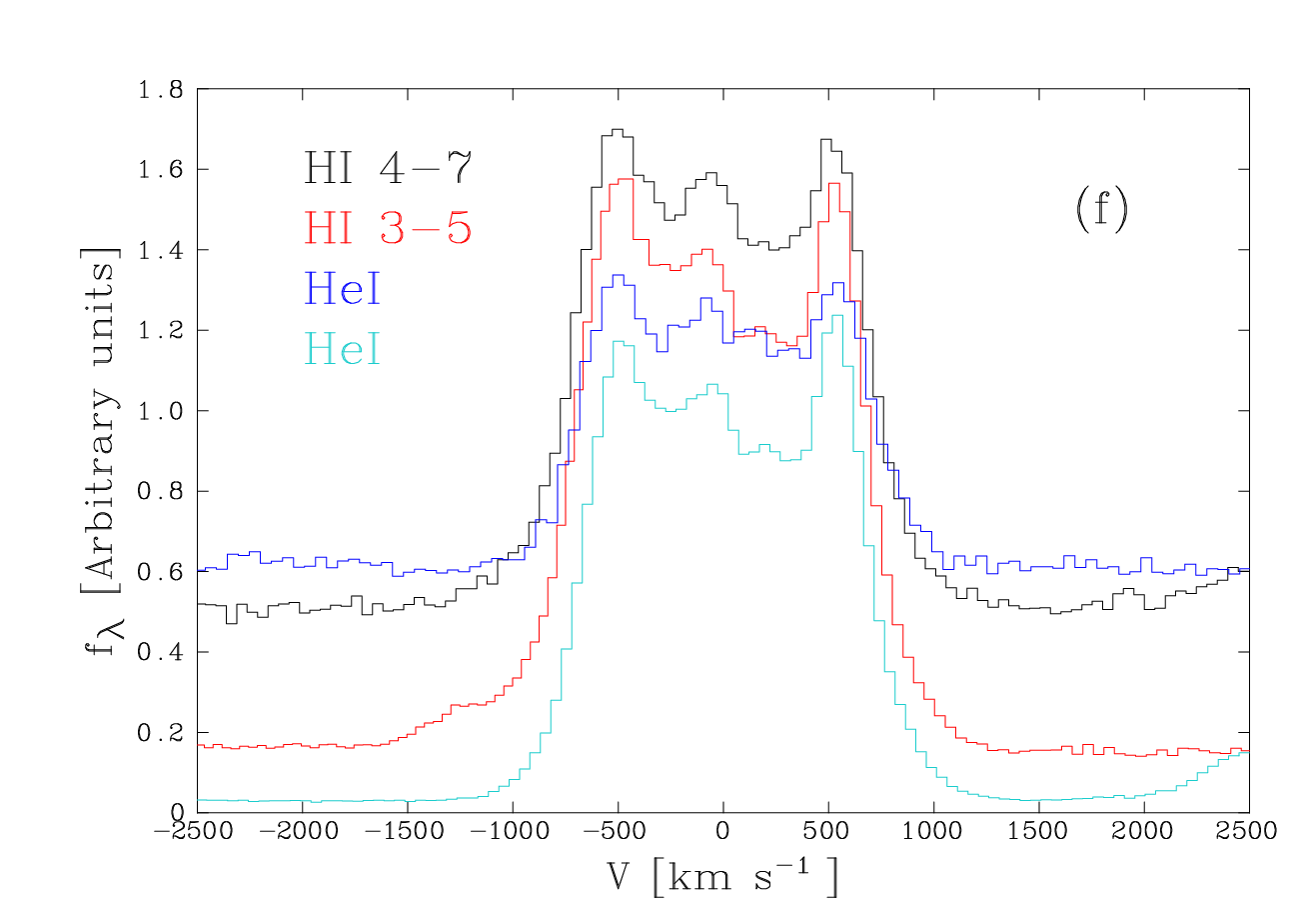
From days, however, there seems to have been a significant change in the profile of the Pa line (Fig. 5(c)-(d)). Prior to day 37 Pa is symmetrical, with HWHM km s-1 but by day 77, there is a distinct asymmetry. A simple Gaussian fit to the Pa line for day 77.79 shows evidence for two distinct features, with HWHM velocites of 418 km s-1 (blue component) and 437 km s-1 (red component), deconvolved for the instrumental resolution. The line centroids are at velocities of km s-1 and km s-1, respectively (Fig. 5(e)). This change in profile coindides with the epoch of maximum dust mass (see Section 5). The data presented here suggest that the torus was obscuring the receding lobe as early as day 77. By day 683.06, however, the blue wing seems to have recovered (see Fig. 5(f)), possibly due to dispersal of the dust or, more likely, due to the destruction of a large fraction of the dust shell (see Section 5.4 below).
4.3 Case B analysis

A recombination Case B analysis was carried out for four epochs (Fig. 6) between 15.8 to 36.8 d after outburst, before dust formation set in. The analysis was along similar lines as for Nova Cep 2014 (Srivastava et al., 2015). Fig.6 shows the Brackett line strengths with respect to Br13 set to unity. The line fluxes do not match predicted Case B values and the Br line strength is significantly lower than the values predicted by Storey & Hummer (1995). This indicates that Br is optically thick, and so possibly are the other Br lines. Similar optical depth effects in the Br lines, due to high plasma densities during the early stages after outburst, is common and has been seen in several other novae e.g. Nova Oph 1998 (Lynch et al., 2000), V2491 Cyg, V597 Pup, RS Oph, T Pyx, Nova Cep 2014 (see Naik et al., 2009; Joshi et al., 2014; Srivastava et al., 2015, and references therein).
| ( M⊙) | m) | |||||||
|---|---|---|---|---|---|---|---|---|
| (days) | ( W m-2) | (K) | BB | AC | GR | AC | GR | |
| 36.82 | 2.97 | 4.29 | ||||||
| 37.69 | 6.72 | 10.64 | ||||||
| 77.79 | 6.46 | 11.93 | ||||||
| 102.14 | 8.47 | 1.07 | ||||||
| 102.66 | 3.66 | 6.74 | ||||||
| 683.06 | 0.54 | 1.23 | ||||||


Following the formalism of Hummer & Storey (1987) and Storey & Hummer (1995), the optical depth at the Br line-center is given by
where and are the electron and ion densities respectively, which are assumed to be equal, and is the opacity corresponding to the transition from upper level to lower level , values of which are listed in Storey & Hummer (1995). The path length is taken as the kinematical distance travelled by the ejecta, where km s-1 is the velocity of ejecta and is the time after outburst. We consider values of between 15.8 day to 36.8 day (from Fig. 6) and set the constraint that be greater than 1. The lower limit on the electron density is then found to be in the range cm-3 to cm-3 on day 15.8. By day 36.8, the density decreases in the range cm-3 to cm-3. These derived lower limits should be smaller than the actual values because can be considerably . An additional caveat in this analysis is the intrinsic assumption of spherical geometry for the ejecta. (Slavin, O’Brien & Dunlop, 1995) since a bipolar morphology appears more appropriate for V339 Del (Schaefer et al., 2014; Shore et al., 2016, see also).
A rough estimate of the ejected mass may be obtained using
where ) is the volume, is the volume filling factor (Shore et al., 2016, assumed from) and is the proton mass. We use the lower limits on estimated above and allow to vary between the distance traversed from 15.8 d to 36.8 d. The lower limit on the mass is estimated to lie between to M⊙. These estimates are roughly a factor of 10 – 20 times lower than the mass estimates given by Gehrz et al. (2015) and Shore et al. (2016), which lie in the range M⊙, but as noted above our values are lower limits.


4.4 Optical Spectra
By day 672 V339 Del had evolved into the nebular phase of its evolution. Our optical spectroscopy (Fig. 4) show at this epoch emission was dominated by recombination lines from the hydrogen Balmer series, helium ions and low ionization, forbidden line emission from metals such as C, N, O, Si, and Fe. The strongest emission lines in the spectra arise from [O iii]4958.91/5006.84 Å. The peak of the emission line profiles exhibit a “double-horn” structure indicating that the total observed emission at a given wavelength arises from material receding from and approaching the observer (i.e., a ring or shell structure to the ejecta).
Using the IRAF SPLOT deblending tool, the components of line profiles were deblended assuming a simple model for the ejecta geometry wherein two Gaussian components were fit to an emission line using the average value of the local continuum using a non-linear least squares technique. Fig. 8 shows the structure of the optical Balmer H line with the two fit velocity components, which are similar to those seen in the infrared Paschen and Brackett series lines depicted in Fig. 5(f) observed on day 683.06. The spectral resolution of the optical and infrared spectra are comparable, and while the velocity peak of the blue shifted material is of the order km s-1, that of the red shifted material differs by km s-1 between the optical and the infrared profiles. However, this is less than the optical velocity resolution ( km s-1) hence we consider the two measurements comparable.
Emission from metal ions also dominates the optical spectra. The strongest of these lines also exhibit emission from two velocity components as seen in the Balmer lines. Fig. 9 shows the Gaussian deblending of the [O iii]4958/5006 Å (rest wavelengths in air) forbidden line profiles with the velocity components marked as well as each Gaussian fit. The sum total of the two components are overlain on the observed emission profiles from the spectra for comparison. Various lines were fit using this technique with integrated line fluxes determined from measurements of the line cores and Gaussian full width half maxima. A detailed description of line identifications derived from the optical spectra on day 672.50 – uncorrected for extinction – is summarised in Table 3 in Appendix A.
Detailed use of the optical and infrared line fluxes observed over multiple epochs as input to photoionization abundance synthesis models is discussed in a forthcoming manuscript.
5 Evolution of the dust


The evolution of the IR spectral energy distribution is shown in Fig. 7. On some of the epochs there is a clear IR excess at the longer wavelengths, which we attribute to the dust reported by Shenavrin et al (2013) and Gehrz et al. (2015); it is also evident that there is a contribution from free-free and free-bound emission, although this becomes less important in the -band. There is no evidence for the presence of dust on or before 2013 September 16 (day 33.75; see Fig. 7).
We attempted to fit a function of the form
to the excess. Here is a scaling factor, is the “-index” for the dust, defined in the usual way such that the dust emisivity is , and is the dust temperature. However, a non-zero value of persistently gave a poor fit for all datasets; best fits were obtained by forcing , i.e. pure black body emission by the dust shell, although this does not of course necessarily imply black body dust grains. The deduced black body temperatures are typically in the range K. At these temperatures peaks around m and the -band data alone are sufficient to pin down the temperature; this is particularly helpful as the free-free emission is (apart from the IRTF spectrum obtained on day 683.06) less prominent at these wavelengths. For example, fitting the black body function to both - and -band spectroscopic data for day 102.66 gives a dust temperature of K, compared with K for the -band data alone (see Table 2); the formal temperature errors are small compared with as a consequence of the large number of data points in the fit. In view of the uncertainties in the flux calibration and in fitting the grain parameters (see below) we do not consider the difference to be significant.
We have therefore fitted the -band data – with emission lines removed – with black bodies; the fits are shown in Fig. 7. The evolution of the temperature and dust flux (as given by ) are listed in Table 2 and shown in Fig. 10(a) and (b) respectively. There is no clear evidence for the presence of dust on 2013 September 16 (day 33.75; see Fig. 7, top right panel); this is consistent with the conclusion of Taranova et al. (2014), who found that dust formation occurred around 2013 September 17. These authors determined a colour temperature of K on 2013 September 21, and K on 2013 October 11, close to the values reported in Table 2.
There remains a weak dust excess on day 683.06 but it is clear from Figs 3 and 7 that free-free and free-bound emission by the gas is comparable with, if not dominating, the dust emission by this time. We have removed the free-free and free-bound emission as determined in Section 3.2 to determine the dust excess, which has a black body temperature of 651 K. There is no trace of dust emission shortward of 2.5m by day 839.30.
5.1 The nature of the dust
To determine the nature of the dust, including dust mass and grain radius, we use the information in Appendix B; this includes a revised Planck Mean absorption efficiency for carbon dust, determined from the data in Blanco, Falcicchia & Merico (1983). The relevant information, including formulae, is given in Appendix B.
5.1.1 Grain radius
To determine grain radius we use Equation (6) of Gehrz et al. (2016), with L⊙ and , where km s-1 (see above).
The dependence of grain radius on time is shown in Fig. 10(c). In reality of course, there will be a distribution of grain sizes (Evans et al., 2005, see e.g.) and the grain size calculated in this way gives an average over the dust shell. However, it seems clear that there is a rapid rise in the grain size immediately following grain formation, eventually followed by a phase in which the grain size diminishes substantially. This is further discussed below.
5.1.2 Dust mass
Black body grains.
For black body (BB) grains the dust mass is given by (see Equation (6))
| (1) |
where we have assumed 1m carbon grains ( g cm-3) and distance kpc. The dust masses are included in Table 2 in the column headed BB; the uncertainties have been propagated from the uncertainties in and . The dependence of dust mass on time is shown Fig. 10(d).
Optically thin amorphous carbon.
Optically thin graphitic carbon.
5.2 Grain temperature and mass
Using the dust temperatures from Table 2, we find that the dust cools according to
| (2) |
with an uncertainty of in the exponent of . Grains having non-zero , flowing at uniform velocity away from a heating source with constant bolometric luminosity (as would be the case for a CN during the evolutionary phase discussed here), would show a dependence; the resultant . This is slightly different from zero at the level and hints at the presence of graphitic () rather than amorphous carbon grains (; see also Fig. 10(a)) but we consider various options below.
We recall that there was no evidence for dust on day 33.75 (see above), when the dust temperature would have been K according to Equation (2); Taranova et al. (2014) concluded that dust formed on day 34.75, giving K. Extrapolation of Equation (2) leads us to conclude that the dust in V339 Del condensed at a temperature of K. Interestingly, this is well within the range of temperatures (1 150 – 1 690 K) at which graphitic carbon condenses in carbon-rich flows (Ebel, 2000, see also discussion in Evans & Rawlings (2008)). This reinforces the conclusion that the dust in V339 Del was graphitic carbon. Furthermore, it is of interest to note that the dust in the classical nova V2326 Cyg condensed at a temperature K (Lynch et al., 2008), close to the value of the dust condensation temperature we have deduced for V339 Del.
There is further, albeit very circumstantial, evidence for carbon dust in the broadband photometry from the O’Brien Observatory, obtained on day 102.14. In these data there seems to be an excess with respect to the black body continuum at m (see Fig. 7), although there was no evidence for a feature in this wavelength range in the SOFIA data on day 27.4 (Gehrz et al., 2015). There are a number of possible sources for this excess on day 102.14. The most plausible assignment would be Hu at 12.3719m ([Ne ii] 12.8135m, although sometimes present even in CO novae (Evans et al., 1997, see e.g.), would need to be implausibly strong to have a significant effect on broadband data). Another alternative, which would be consistent with the presence of carbon dust, is the 11.1/12.7m CH out-of-plane bending modes in polycyclic aromatic hydrocarbons, commonly seen in nova dust (see e.g. Helton et al., 2011, and references therein).
Irrespective of dust composition, there seems to be some evidence for an increase in dust mass up to day 100, followed by a substantial decline to day . The increase may be attributed to grain growth, an increase in the number of emitting grains, or a combination of both these effects. Conversely the subsequent decline must be due to a decline in grain size or decrease in grain number, either of which points to grain destruction on a substantial scale.
5.3 A dust minimum in the visual light curve
It is of interest to correlate the evolution of the dust with the behaviour of the visual light curve. Following visual maximum, the light curve declines uniformly, but the decline becomes distinctly slower after ( day 12; see Fig. 1(a)); then there is a distinct dip in the light curve as dust forms. We have fitted the light curve immediately before and after the dust dip with a function of the form
and find and day-1 (note that must not be associated with the “speed class” of the nova). We rectified the light curve with this decline to highlight the dust dip (see Fig. 1(b), in which the dust optical depth is plotted against the Julian Date). There is a clear maximum in , with , around JD 2 456 580 ( day 62). Within the limitations of the cadence of the IR observations, this coincides with maximum grain size and maximum grain mass in Fig. 10(c,d); the duration of the dust phase, as determined by the IR observations, is consistent with the width of the dust dip in Fig. 1(b).
5.4 Grain destruction
Evidence for grain destruction in a nova wind was first noted in the case of nova LW Ser (1978) by Gehrz et al. (1980a). The physical processes associated with grain destruction in nova winds have been discussed by Mitchell, Evans & Bode (1983), Mitchell & Evans (1984), Mitchell, Evans & Albinson (1986) and Rawlings & Evans (1995), in the context of sputtering and chemi-sputtering of carbon dust, and the effect of annealing carbon dust in the UV radiation field of the nova.
However, more recently the effect of X-radiation on the survival of dust has been the subject of considerable interest in the context of -ray bursts (Fruchter et al., 2001), and as V339 Del was an X-ray source (see Section 1), it is of interest to consider the effect of hard radiation on the survival potential of dust in the environment of V339 Del.
Fruchter et al. (2001) considered the competition between the input of energy into grains by X-radiation, and energy loss by grain radiation and sublimation. They also considered the effect of grain shattering due to electrostatic stress, resulting from grain charging following the ejection of electrons from the shell of atoms within the grain.
We see from Fig. 10 that, when the dust mass peaked around day 100, the dust temperature was K and steadily declined thereafter; is seems unlikely therefore that, at K, graphitic grains – for which the sublimation temperature is K for carbon-rich environments (Lodders & Fegley, 1995) – would be subject to evaporation: it is more likely that it is grain shattering by electrostatic stress that destroyed the grains around V339 Del.
Fruchter et al. (2001) found that, whether or not a grain survives following exposure to X-radiation is determined by the parameter , where is the energy radiated in the form of X-rays at 1 keV, normalised to ergs, and is the distance of the grains from the X-ray source in units of 100 pc; from Figure 1 of Fruchter et al., grains are shattered if .
We suppose that, at the time of maximum grain size, the nova was a SSS with the bulk of the radiation being emitted at X-ray wavelengths. Assuming that the grains are exposed to X-rays for a time , at time after the eruption, the Fruchter et al. parameter is
where is the fraction of the nova radiation emitted at 1 keV. Taking L⊙ (Gehrz et al., 2015), km s-1, days, days, we find . So if , which seems reasonable, charging of grains by X-radiation is more than sufficient to shatter the grains.
However, while it seems that exposure to X-radiation would destroy the dust, we should express a note of caution in that the Fruchter et al. analysis assumes a power-law for the X-ray source; while this would be valid for the hard X-radiation, it is less so for the near-black body X-ray source appropriate for a CN during the SSS phase (even though pure black body emission does not generally provide a good description of the SSS phase of novae). This issue will be addressed in a forthcoming paper.
Finally, we speculate that the shattering of micron-sized graphitic grains in the way we have suggested might result in the release of significant amounts of polycyclic aromatic hydrocarbon (PAH) fragments, possibly even fullerenes, into the nova environment. If this is the case classical novae may display persistent PAH emission (see Helton et al., 2011, for a summary of PAH emission in novae) for some time after the dust formation phase has apparently come to an end.
6 Conclusions
We have presented infrared spectroscopy of the classical nova V339 Del.
The IR spectrum is initially dominated by emission by the ejected gas, with H i and low excitation atomic CNO lines being prominent. There is clear evolution in the emission line profiles. The lines are initially ( days) symmetric, with HWHM km s-1. However, after day 77, they become highly asymmetric, with a strong blue and weak red wing. Later still ( days) the emission lines display a castellated structure.
Rapid dust formation occurs around day 34.75, following which the IR emission becomes dominated by the dust. The dust condensation temperature was K, consistent with the notion that the dust is graphitic. We find that M⊙ of dust was formed, and that the grains grew to a dimension of a few m. We further find that both the mass of dust, and the radius of the dust grains, increased rapidly following the formation of dust, peaked around 100 days after eruption, and thereafter declined precipitously. We attribute this to the charging of dust grains by the X-ray emission of V339 Del, causing the grains to shatter due to electrostatic stress.
Acknowledgements
We thank Dr Kim Page for valuable information about the early X-ray emission of V339 Del, and the British Astronomical Association and The Astronomer magazine for providing its visual light curve. We also appreciate the referee’s supportive comments on this paper.
RDG acknowledges support from the National Aeronautics and Space Administration (NASA) and the United States Air Force. VARMR acknowledges financial support from the Radboud Excellence Initiative. CEW acknowledges partial support from NASA (HST-GO-13828.008-A). SS gratefully acknowledges partial support from both NASA and NSF grants to ASU. The research work at the Physical Research Laboratory is supported by the Department of Space, Government of India. DS is a visiting astronomer at the Infrared Telescope Facility which is operated by the University of Hawaii under contract NNH14CK55B with NASA.
References
- Ackermann et al. (2014) Ackermann M., et al., 2014, Science, 345, 554
- Ahnen et al. (2015) Ahnen M. L., 2015, A&A 582, A67
- Banerjee & Ashok (2012) Banerjee D. P. K., Ashok N. M., 2012, BASI, 40, 243
- Banerjee et al. (2013a) Banerjee D. P. K., Ashok N. M., Joshi V., Evans A., 2013a, ATel 5337
- Banerjee et al. (2013b) Banerjee D. P. K., Ashok N. M., Joshi V., Evans A., 2013b, ATel 5404
- Banerjee et al. (2016) Banerjee D. P. K., Srivastava Mudit K., Ashok N. M., Venkataraman V., 2016, MNRAS, 455, L109
- Beardmore, Osborne & Page (2013) Beardmore A. P., Osborne J. P., Page K. L., 2013, ATel 5573
- Becklin & Capps (1981) Becklin E. E., Capps R. W., 1981, Proc. SPIE, 263, 58
- Blanco et al. (1983) Blanco A., Falcicchia G., Merico F., 1983, Ap. & Sp. Sci., 89, 163
- Bode & Evans (2008) Bode M. F., Evans, A., 2008, Eds Classical Novae, second edition, Cambridge University Press
- Cass et al. (2013a) Cass A. C., Carlon R. L., Corgan D. T., Dykhoff D. A., Gehrz R. D, Shenoy D. P., 2013a, ATel 5434
- Cass et al. (2013b) Cass A. C., Carlon R. L., Corgan D. T., Dykhoff D. A., Gehrz R. D, Shenoy D. P., 2013b, ATel 5604
- Chomiuk et al. (2014) Chomiuk L., et al., 2014, Nature, 514, 339
- Currie et al. (2014) Currie M. J., Berry D. S., Jenness T., Gibb A. G., Bell G. S., Draper P. W., 2014, in Astronomical Data Analysis Software and Systems XXIII, eds N. Manset and P. Forshay, Astronomical Society of the Pacific Conference Series, 485, 391
- Cushing, Vacca & Rayner (2004) Cushing, M. C., Vacca, W.D., Rayner, J. T., 2004, PASP, 116, 362
- Darnley et al. (2013) Darnley M. J., Bode M. F., Smith R. J., Evans A., 2013, ATel 5279
- Das et al. (2009) Das R. K., Banerjee D. P. K., Ashok, N. M., 2009, MNRAS, 398, 375
- Deacon et al. (2014) Deacon N. R., et al., 2014, A&A 563, A129
- Ebel (2000) Ebel D. S., 2000, J. Geophys. Res., 105 10363
- Evans & Rawlings (1994) Evans A., Rawlings J. M. C., 1994, MNRAS, 269, 427
- Evans et al. (1996) Evans A., Geballe T. R., Rawlings J. M. C., Scott A. D., 1996, MNRAS, 282, 1049
- Evans et al. (1997) Evans A., Geballe T. R., Rawlings J. M. C., Eyres S. P. S., Davies J. K., 1997, MNRAS, 292, 192
- Evans et al. (2005) Evans A., Tyne V. H., Smith O., Geballe T. R., Rawlings J. M. C., Eyres S. P. S., 2005, MNRAS, 360, 1483
- Evans & Gehrz (2012) Evans A., Gehrz R. D., 2012, BASI, 40, 213
- Evans & Rawlings (2008) Evans A., Rawlings J. M. C., 2008, in Classical Novae, second edition, eds M. F. Bode, A. Evans, Cambridge University Press
- Fruchter et al. (2001) Fruchter A., Krolik J. H., Rhoads J. E., 2001, ApJ, 563, 597
- Gehrz & Ney (1992) Gehrz R. D., Ney E. P., 1992, Icarus, 100, 162
- Gehrz et al. (1980a) Gehrz R. D., Grasdalen G. L., Hackwell J. A., Ney E. P., 1980a, ApJ, 237, 855
- Gehrz et al. (1980b) Gehrz R. D., Hackwell J. A., Grasdalen G. I., Ney E. P., Neugebauer G., Sellgren K., 1980b, ApJ, 239, 570
- Gehrz (2008) Gehrz R. D., 2008, in Classical Novae, Eds M. F. Bode, Evans, p. 167, Cambridge University Press
- Gehrz et al. (2014) Gehrz R. D., Evans A., Woodward C. E., 2014, in Stella Novae: Future and Past Decades, eds. P. A. Woudt and V. A. R. M. Ribeiro, Astronomical Society of the Pacific Conference Series, 490, 227.
- Gehrz et al. (2015) Gehrz R. D., et al., 2015, ApJ, 812, 132
- Gehrz et al. (2016) Gehrz R. D., et al., 2016, submitted
- Gilman (1974) Gilman R. C., 1974, ApJS, 28, 397
- Haenecour et al. (2016) Haenecour P., Floss C., José, J., Amari S., Lodders K., Jadhav M., Wang A., Gyngard F., 2016, ApJ, 825, 88
- Hays et al. (2013) Hays E., Cheung T., Ciprini S, 2013 ATel 5302
- Helton et al. (2011) Helton L. A., Evans A., Woodward C. E., Gehrz, R. D., 2011, in PAHs and the Universe, eds C. Joblin and A. G. G. M. Tielens, EAS Publications Series, 46, 407
- Helton et al. (2012) Helton L. A., et al., 2012, ApJ, 755, 37
- Howarth et al. (2004) Howarth I. D., Murray J., Mills D., Berry D. S., 2004, DIPSO – A friendly spectrum analysis program, Starlink User Note 50.24
- Hummer & Storey (1987) Hummer D. G., Storey P. J., 1987, MNRAS, 224, 801
- Joshi et al. (2014) Joshi V., Banerjee D. P. K., Ashok N. M., 2014, MNRAS, 443, 559
- Krautter (2008) Krautter J., 2008, in Classical Novae, Eds M. F. Bode, A. Evans, p. 232, Cambridge University Press
- Kuulkers et al. (2013) Kuulkers E., Page K. L., Osborne J. P., Kuin N. P. M., Sokolovsky K. V., Ness J.-U., 2013, ATel 5283
- Linford et al. (2015) Linford J. D., et al., 2015, ApJ, 805, 136
- Lodders & Fegley (1995) Lodders K., Fegley B., 1995, Meteoritics, 30, 661
- Lynch et al. (2000) Lynch D. K., Rudy R. J., Mazuk S., Puetter R. C., 2000, ApJ, 541, 791
- Lynch et al. (2008) Lynch D. K., et al., 2008, AJ, 136, 1815
- Martin & Dubus (2013) Martin P., Dubus G., 2013, A&A, 551, A37
- Mitchell, Evans & Bode (1983) Mitchell R. M., Evans A., Bode M. F., 1983, MNRAS, 205, 1141
- Mitchell & Evans (1984) Mitchell R. M., Evans A., 1984, MNRAS, 209, 945
- Mitchell et al. (1986) Mitchell R. M., Evans A., Albinson J. S., 1986, MNRAS, 221, 663
- Munari et al. (2013a) Munari U., et al., 2013a, ATEL 5927
- Munari et al. (2013b) Munari U., Henden A., Dallaporta S., Cherini G., 2013b, IBVS 6080
- Naik et al. (2009) Naik S., Banerjee D. P. K., Ashok N. M., 2009, MNRAS, 394, 1551
- Nakano et al. (2013) Nakano S., et al., 2013, CBET 3628
- Ness et al. (2013) Ness J.-U., Schwarz G. J., Page K. L., Osborne J. P., Bode M. F., Shore, S. N., van Rossum D., Starrfield S., Walter F., Woodward C. E., 2013, ATel 5626
- Osterbrock & Ferland (2006) Osterbrock D. E., Ferland G. J., 2006, Astrophysical of Gaseous Nebulae and Active Galactic Nuclei, University Science Books
- Page & Beardmore (2013) Page K. L., Beardmore A. P., 2013, ATel 5429
- Page et al. (2013a) Page K. L., Osborne J. P., Beardmore A. P., Kennea J. A., 2013a, ATel 5318
- Page et al. (2013b) Page K. L., Osborne J. P., Kuin N. P. M., Woodward C. E, Schwarz G. J., Starrfield S., Shore S. N., Walter F. M., 2013b, ATel 5470
- Payne-Gaposchkin (1957) Payne-Gaposchkin C., 1957, The Galactic Novae, Dover Publications, New York
- Pepin et al. (2011) Pepin R. O., Palma R. L., Gehrz R. D., Starrfield S., 2011, ApJ, 742, 86
- Raj et al (2012) Raj A., Ashok N. M., Banerjee D. P. K., Munari U., Valisa P., Dallaporta S., 2012. MNRAS, 425, 2576
- Rawlings & Evans (1995) Rawlings J. M. C., Evans A., 1995, Astrophys. Space Sci., 224, 543
- Rayner et al. (2003) Rayner J. T., Toomey D. W., Onaka P. M., Denault A. J., Stahlberger W. E., Vacca W. D., Cushing M. C., Wang, S.,2003, PASP,115, 805,362
- Ribeiro, Munari & Valisa (2013) Ribeiro V. A. R. M., Munari U., Valisa P., 2013, ApJ, 768, 49
- Rudy et al. (2003) Rudy R. J., Dimpfl W., Lynch D. K., Mazuk S., Venturini C. C., Wilson J. C., Puetter R. C., Perry R. B., 2003, ApJ, 596, 1229
- Saikia & Anupama (2012) Saikia D. J., Anupama G. C., 2012, Eds Novae from radio to gamma rays, special edition of the Bulletin of the Astronomical Society of India
- Schaefer et al. (2014) Schaefer G. H., et al. 2014, Nature, 515, 234
- Schmidt et al. (1989) Schmidt G. D., Weymann R. J., Foltz C. B., 1989, PASP, 101, 713
- Shenavrin et al (2013) Shenavrin V. I., Taranova O. G., Tatarnikov, A. M., 2013, ATel 5431
- Shore et al. (2013) Shore S. N., De Gennaro Aquino I., Schwarz G. J., Augusteijn T., Cheung C. C., Walter F. M., Starrfield S., 2013, A&A, 553, A123
- Shore et al. (2014) Shore S. N., De Gennaro Aquino I., Scaringi S., van Winckel H., 2014, A&A, 570, L4
- Shore et al. (2016) Shore S. N., et al., 2016, A&A, 590, A123
- Slavin, O’Brien & Dunlop (1995) Slavin A. J., O’Brien T. J., Dunlop J. S., 1995, MNRAS, 276, 353
- Skopal et al. (2014) Skopal A., et al., 2014, A&A, 569, A112
- Srivastava et al. (2015) Srivastava M., Ashok N. M., Banerjee D. P. K., Sand D., 2015, MNRAS, 454, 1297
- Starrfield, Iliadis & Hicks (2016) Starrfield S., Iliadis C., Hix W. R., 2016, PASP, 128, 051001
- Storey & Hummer (1995) Storey P. J., Hummer D. G., 1995, MNRAS, 272, 41
- Stringfellow, Hebb & Fumagalli (2013) Stringfellow G. S., Hebb L., Fumagalli M., 2013, ATel 5336
- Taranova et al. (2014) Taranova O. G., Tatarnikov A. M., Shenavrin V. I., Tatarnikova, A. A., 2014, Astron. Lett., 40, 120
- Tarasova & Skopal (2014) Tarasova T. N., Skopal A., 2016, Astron. Lett., 42, 10
- Tatischeff & Hernanz (2007) Tatischeff V., Hernanz M., 2007, ApJ, 663, L101
- Vacca et al. (2003) Vacca, W. D., Cushing, M. C., Rayner, J. T., 2003, PASP, 115, 389
- Warner (2008) Warner B., 2008, in Classical Novae, Eds M. F. Bode, A. Evans, p. 16, Cambridge University Press
- Weingartner et al. (2006) Weingartner J. C., Draine B. T., Barr D. T., 2006, ApJ, 645, 1188
- Williams (1992) Williams R. E., 1992, AJ, 104, 725
- Williams (2012) Williams R., 2012, AJ, 144, 98
- Williams et al. (2013) Williams S. C., Bode M. F., Darnley M. J., Evans A., Zubko V., Shafter A. W., 2013, ApJ, 777, L32
- Woudt & Riberio (2014) Woudt, P. A., Ribeiro V. A. R. M., eds Stella Novae: Past and Future Decades, Astronomical Society of the Pacific Conference Series, Volume 490
- Young et al. (2012) Young E. T., et al., 2012, ApJ, 749, L17
Appendix A Observed line fluxes
A.1 Mt Abu data
The line centres and fluxes were determined by subtracting a continuum and fitting Gaussian functions to the emission line profiles. The uncertainties in the line centres and fluxes arise from the placement of the continuum and the Gaussian fitting. Repeated experiments with slight variations in the assumed continuum, and comparison with line fitting on different dates, showed that the uncertainties in the line centres are typically m, and % to in the line fluxes.
The line fluxes are listed in Table 1, which lists data to day 26.70, and Table 2, which lists data from day 27.76 onwards. Both Tables give measured wavelengths, suggested identifications and transitions.
| ID, | Transition | Line flux ( W m-2) on days given | |||||||||
|---|---|---|---|---|---|---|---|---|---|---|---|
| (m) | (m) | ||||||||||
| 14.76 | 15.79 | 19.78 | 20.73 | 22.73 | 24.72 | 25.75 | 26.70 | ||||
| 1.0828 | He i, 1.0833 | 3SPo | – | – | – | – | – | – | – | – | – |
| 1.0936 | H i, 1.0941 | 3–6 | – | 153(5) | – | – | 82.7(36) | 109(5) | 99.3(57) | 105(7) | – |
| 1.0946 | N i, 1.0946 | 4SP | – | – | – | – | – | – | – | 122(95) | |
| 1.1284 | C i, 1.1281 | 1DF | – | – | – | – | – | – | – | 470(8) | – |
| 1.1293 | O i, 1.1290 | 3PDo | – | – | – | 320(5) | 313(4) | 456(6) | 392(7) | – | 469(11) |
| 1.1300 | N i, 1.1297 | 4DP1/2 | – | 353(8) | 433(9) | – | – | – | – | – | – |
| O i, 1.1301 | 5PS | – | – | – | – | – | – | – | – | – | |
| C i, 1.1301 | 3PD2 | – | – | – | – | – | – | – | – | – | |
| N i, 1.1301 | 4PP1/2 | – | – | – | – | – | – | – | – | – | |
| N i, 1.1300 | 4PD | – | – | – | – | – | – | – | – | – | |
| N i, 1.1303 | 2PD | – | – | – | – | – | – | – | – | – | |
| N i, 1.1304 | 4DD1/2 | – | – | – | – | – | – | – | – | – | |
| 1.1463 | – | – | – | – | – | – | – | – | – | ||
| 1.1619 | C i, 1.1618 | 3DDo | – | – | 24.2(12) | 9.17(69) | – | – | 3.92(50) | – | – |
| C i, 1.1622 | 3DDo | – | – | – | – | – | – | – | – | – | |
| 1.1654 | C i, 1.1651 | 3DD | – | 75.2() | – | 29.3(36) | 27.9(16) | 35.0(92) | 24.2(1.63) | 26.4(1.3) | 31.7(94) |
| 1.1662 | C i, 1.1662 | 3SPo | – | 48.0(58) | – | – | – | – | – | – | |
| 1.1758 | C i, 1.1758 | 3DF | – | 151(3) | 160(4) | 91.5(18) | 76.5(35) | 92.5(18) | 73.7(11) | 74.9(14) | 80.4(10) |
| C i, 1.1757 | 3DF | – | – | – | – | – | – | – | – | – | |
| 1.1863 | C i, 1.1864 | 3PD | – | 49.4(25) | – | – | – | – | – | – | – |
| C i, 1.1864 | 3PD | – | – | – | – | – | – | – | – | – | |
| C i, 1.1866 | DP | – | – | – | – | – | – | – | – | – | |
| N i, 1.1861 | 4SP3/2 | – | – | – | – | – | – | – | – | – | |
| 1.1887 | – | – | – | 16.3(13) | 18.2(18) | 21.9(11) | 16.8(7) | 13.7(9) | 19.7(10) | ||
| 1.2087 | – | – | – | – | – | – | – | – | 12.5(14) | ||
| 1.2191 | – | – | – | – | – | – | – | – | 4.19(34) | ||
| 1.2300 | – | – | – | – | – | – | – | – | 8.76(51) | ||
| 1.2466 | N i, 1.2473 | 2DF7/2 | – | 26.4(52) | 31.8 (37) | 10.5(13) | 11.4(23) | 11.7(8) | 11.5(15) | 11.0(14) | 11.2(10) |
| ID, | Transition | Line flux ( W m-2) on days given | |||||||||
|---|---|---|---|---|---|---|---|---|---|---|---|
| (m) | (m) | ||||||||||
| 14.76 | 15.79 | 19.78 | 20.73 | 22.73 | 24.72 | 25.75 | 26.70 | ||||
| 1.2509 | – | – | – | – | – | – | – | – | – | ||
| 1.2586 | N i, 1.2586 | 2FDo | – | 46.5(10) | 49.1(11) | 17.6(16) | 17.3(28) | 17.6(10) | 17.1(38) | 16.5(4) | 14.7(10) |
| C i, 1.2585 | 3PP | – | – | – | – | – | – | – | – | – | |
| N i, 1.2585 | 2DF5/2 | – | – | – | – | – | – | – | – | – | |
| 1.2809 | – | – | – | – | – | – | – | – | – | ||
| 1.2823 | H i, 1.2822 | 3–5 | 8.40(107) | 213(3) | 261(4) | 175(2) | 170(3) | 198(2) | 202(2) | 218(2) | 224(2) |
| 1.2975 | N i, 1.2973 | 2PDo | – | 3.582(32) | – | – | – | – | – | – | |
| 1.3172 | N i, 1.3177 | 2DD | – | 29.0(6) | – | 14.3(14) | 11.9(23) | – | 13.0(15) | 13.0(15) | 15.2(18) |
| N i, 1.3176 | 2DD | – | – | – | – | – | – | – | – | – | |
| 1.5268 | – | – | – | 1.29(9) | – | – | – | – | 1.77(10) | ||
| 1.5348 | – | – | 3.46(20) | 1.82(11) | – | – | 1.81(8) | – | 1.77(9) | ||
| 1.5447 | – | – | 4.84(20) | 2.80(12) | – | 3.06(14) | 2.56(8) | 2.54(14) | 2.33(9) | ||
| 1.5568 | H i,1.5561 | 4–16 | – | 9.23(28) | 9.64(22) | 5.56(13) | – | 6.33(15) | 5.92(10) | 6.18(17) | 5.67(11) |
| 1.5707 | H i,1.5705 | 4–15 | – | 7.88(31) | 9.07(24) | 5.14(14) | – | 5.82(16) | 5.39(10) | 4.99(17) | 4.58(10) |
| 1.5748 | – | – | – | – | – | – | – | – | – | – | |
| 1.5789 | – | – | 1.47(16) | 0.71(9) | – | 0.69(7) | 0.58(7) | 0.55 (7) | – | ||
| 1.5847 | H i,1.5885 | 4–14 | – | 11.9(3) | 12.3(2) | 6.63(13) | – | 6.55(15) | 6.19(9) | 5.95(16) | – |
| 1.6021 | – | 7.68(28) | 7.75(23) | 3.37(9) | – | 3.12(7) | 2.89(7) | 2.85(7) | 2.95(16) | ||
| 1.6054 | – | – | – | – | – | – | – | – | – | – | |
| 1.6115 | H i, 1.6114 | 4–13 | – | 10.7(2) | 11.3(2) | 6.58(14) | – | 6.63(15) | 6.87(10) | 7.05(17) | 6.69(17) |
| 1.6329 | – | – | – | 0.44(9) | – | – | – | – | – | ||
| 1.6142 | – | – | – | – | – | – | – | – | – | – | |
| 1.6416 | H i, 1.6412 | 4–12 | – | 21.8(5) | 21.67(113) | 10.2(3) | – | 10.5(6) | 10.4(4 ) | 10.3(2) | 10.5(2) |
| 1.6499 | – | – | – | – | – | 0.69(7) | – | – | – | ||
| 1.6711 | – | – | – | 0.95(7) | – | – | – | – | – | ||
| 1.6808 | H i, 1.6811 | 4–11 | – | 19.7(31) | 15.3(7) | 9.38(28) | – | 10.5(4) | 10.6(3) | 10.2(3) | 11.7(6) |
| 1.6826 | – | – | – | – | – | – | – | – | – | ||
| 1.6892 | C i, 1.6895 | 1DF | 2.69(25) | 28.0(29) | 44.4(10) | – | – | 22.1(9) | 23.3(4) | 21.9(5) | 18.8(5) |
| 1.7058 | – | – | – | 1.57(9) | – | – | – | – | – | ||
| 1.7244 | – | – | – | – | – | – | – | – | – | ||
| 1.7251 | – | – | – | 3.71(25) | – | 3.59(39) | 3.29(41) | 2.71(30) | 2.72(16) | ||
| 1.7362 | H i, 1.7367 | 4–10 | – | – | – | 22.5(4) | – | 25.4(11) | 24.7(5) | 23.1(6) | 19.0(6) |
| 1.7450 | – | – | – | – | – | 13.0(5) | – | 11.0(2) | – | ||
| 1.7563 | – | – | – | – | – | 4.53(29) | – | 4.75(21) | – | ||
| 1.7667 | – | – | – | – | – | 11.6(10) | 9.52(50) | 7.98(63) | – | ||
| 1.9741 | – | – | – | 1.71(6) | – | 1.25(6) | 2.19(10) | 1.43(4) | – | ||
| 2.0599 | He i, 2.0587 | 1SP | – | – | – | 1.546) | 2.13(9) | 1.26(9) | 1.77(8) | 1.90(8) | 1.87(7) |
| 2.0757 | – | – | – | 0.32(4) | 0.37(7) | – | – | – | – | ||
| 2.0890 | – | – | – | 0.47(0.04) | 0.70(8) | – | 0.66(4) | 0.54(4) | 0.81(4) | ||
| 2.1029 | C i, 2.1029 | 1SPo | – | 1.50(14) | 2.21(17) | 0.66(4) | 0.74(5) | – | 0.45(3) | 0.35(3) | 0.43(4) |
| 2.1235 | – | 5.85(23) | 7.34(13) | 2.81(6) | 3.07(7) | 2.56(9) | 2.76(7) | 2.24(5) | 2.13(6) | ||
| 2.1492 | – | – | 3.32(12) | – | – | 1.28(7) | 1.33(6) | – | 0.76(3) | ||
| 2.1505 | =[ii0– | – | – | – | 1.46(6) | – | – | 1.01(4) | – | ||
| 2.1645 | – | – | – | – | – | – | – | – | – | – | |
| 2.1667 | H i, 2.1661 | 4–7 | — | 22.5(35) | 20.9(2) | – | 15.3(2) | 14.1(2) | 18.0(2) | 15.5(2) | 16.6(3) |
| 2.2153 | – | 2.44(18) | 1.87(17) | 0.56(5) | – | – | 0.41(3) | 0.28(3) | 0.44(5) | ||
| 2.2891 | – | 1.17(13) | – | – | – | – | – | – | – | ||
| 2.2918 | C i 2.2913 | 1SP | – | – | 2.33(18) | 1.12(5) | – | – | 0.86(32) | 0.73(3) | 0.76(4) |
| 2.3158 | – | – | 0.63(8) | – | – | – | – | – | – | ||
| ID, | Transition | Line flux ( W m-2) on days given | |||||||||
|---|---|---|---|---|---|---|---|---|---|---|---|
| (m) | (m) | ||||||||||
| 31.82 | 33.75 | 36.82 | 37.69 | 77.79 | 78.71 | 101.72 | 102.66 | ||||
| 1.0828 | He i, 1.0833 | 3SPo | – | – | – | 192(3) | 150(2) | – | 8.57(74) | 6.89(16) | 6.89(23) |
| 1.0936 | H i, 1.0941 | 3–6 | – | 183(8) | – | 149(3) | 135(2) | – | – | 1.21(17) | 0.35(11) |
| 1.0946 | N i, 1.0946 | 4SP | – | – | – | – | – | – | – | – | 0.36(10) |
| 1.1284 | C i, 1.1281 | 1DF | 425(4) | 798(9) | – | – | 625(5) | 1.75 (7) | 1.61(7) | 0.82(3) | 0.71(3) |
| O i, 1.1290 | 3PDo | – | – | – | – | – | – | – | – | – | |
| 1.1300 | N i, 1.1297 | 4DP1/2 | – | – | – | – | – | – | – | – | – |
| O i, 1.1301 | 5PS | – | – | – | – | – | – | – | – | – | |
| C i, 1.1301 | 3PD2 | – | – | – | – | – | – | – | – | – | |
| N i, 1.1301 | 4PP1/2 | – | – | – | – | – | – | – | – | – | |
| N i, 1.1300 | 4PD | – | – | – | – | – | – | – | – | – | |
| N i, 1.1303 | 2PD | – | – | – | – | – | – | – | – | – | |
| N i, 1.1304 | 4DD1/2 | – | – | – | – | – | – | – | – | – | |
| 1.1463 | – | – | – | – | – | 0.168(55) | – | – | – | ||
| 1.1619 | C i, 1.1618 | 3DDo | – | – | – | – | – | – | – | – | – |
| C i, 1.1622 | 3DDo | – | – | – | – | – | – | – | – | – | |
| 1.1654 | C i, 1.1651 | 3DD | 18.8(35) | 25.0(18) | 23.4(10) | – | 17.0 (6) | – | – | – | – |
| 1.1662 | C i, 1.1662 | 3SPo | – | – | – | – | – | – | – | – | – |
| 1.1758 | C i, 1.1758 | 3DF | 56.5(31) | 73.0(87) | 67.5(24) | – | 50.3(53) | 0.18(6) | 0.31(8) | 0.14(3) | – |
| C i, 1.1757 | 3DF | – | – | – | – | – | – | – | – | – | |
| 1.1863 | C i, 1.1864 | 3PD | – | – | – | – | – | – | – | – | – |
| C i, 1.1864 | 3PD | – | – | – | – | – | – | – | – | – | |
| C i, 1.1866 | DP | – | – | – | – | – | – | – | – | – | |
| N i, 1.1861 | 4SP3/2 | – | – | – | – | – | – | – | – | – | |
| 1.1887 | 11.3(35) | 30.7(47) | 19.6(11) | – | 11.6(6) | – | – | 0.096(30) | – | ||
| 1.2087 | – | – | 18.1(16) | – | 4.34(62) | – | – | – | – | ||
| 1.2191 | – | – | – | – | – | – | – | – | – | ||
| 1.2300 | – | 3.52(32) | – | – | – | – | – | – | – | ||
| 1.2466 | N i,1.2473 | 2DF7/2 | 7.24(93) | 10.0(12) | 14.3(11) | 7.35(51) | 8.56(18) | – | – | – | |
| 1.2509 | – | – | – | – | – | – | – | – | 0.20(2) | ||
| 1.2586 | N i, 1.2586 | 2FD | 11.3(12) | 13.0(3) | 18.2(14) | 9.82(69) | 11.0(2) | – | – | – | – |
| C i, 1.2585 | 3PP | – | – | – | – | – | – | – | – | – | |
| N i, 1.2585 | 2DF | – | – | – | – | – | – | – | – | – | |
| 1.2809 | – | – | – | – | – | 1.63(5) | 1.77(5) | 1.54(4) | 1.57(3) | ||
| 1.2823 | H i, 1.2822 | 3–5 | 192(2) | 230(1) | 252(3) | 214(2) | 251(1) | – | – | – | – |
| 1.2975 | N i, 1.2973 | 2PDo | – | – | – | – | – | – | – | – | – |
| 1.3172 | N i, 1.3177 | 2DD | 11.1 (11) | 8.9(12) | – | 8.42(65) | 10.6(2) | – | – | – | – |
| N i, 1.3176 | 2DD | – | – | – | – | – | – | – | – | – | |
| 1.5268 | – | – | – | – | – | – | 0.42(4) | – | – | – | – |
| 1.5348 | 1.74(10) | 1.4 (1) | 1.23(8) | – | 0.88(5) | – | – | – | – | ||
| 1.5447 | 2.45(10) | 1.74(10) | 1.79(8) | – | 1.29(5) | – | – | – | – | ||
| 1.5568 | H i, 1.5561 | 4–16 | 5.68(12) | 4.79 (12) | 4.28(9) | 3.40(7) | 3.13(6) | – | – | – | – |
| 1.5707 | H i, 1.5705 | 4–15 | 4.67(12) | 4.03(12) | 3.68(9) | 2.86(2) | 2.18(5) | – | – | – | – |
| 1.5748 | – | – | – | – | – | – | – | – | 0.025(4) | ||
| 1.5789 | – | – | – | – | – | – | – | – | – | ||
| 1.5847 | H i, 1.5885 | 4–14 | 5.44(11) | 4.37(11) | 4.14(9) | 3.29(7) | 3.31(8) | 0.17(1) | – | – | 0.119(14) |
| 1.6021 | 2.53(10) | 1.48(10) | 1.26(8) | 0.90(6) | 0.99(7) | – | – | – | – | ||
| 1.6054 | – | – | – | – | – | – | – | – | 0.027(3) | ||
| 1.6115 | H i, 1.6114 | 4–13 | 6.28(11) | 5.30(12) | 4.53(9) | 3.94(7) | 3.52(8) | – | – | – | – |
| 1.6142 | – | – | – | – | – | – | – | – | 0.092(16) | ||
| 1.6329 | – | – | – | – | – | – | – | – | – | ||
| 1.6416 | H i, 1.6412 | 4–12 | 8.60(15) | 7.65 (12) | 6.93(16) | 5.86(56) | 5.62(8) | – | – | – | 0.183(16) |
| 1.6499 | – | – | 0.318(66) | – | – | – | – | – | – | ||
| 1.6711 | – | – | 0.428(72) | – | – | – | – | – | – | ||
| ID, | Transition | Line flux ( W m-2) on days given | |||||||||
|---|---|---|---|---|---|---|---|---|---|---|---|
| (m) | (m) | ||||||||||
| 31.82 | 33.75 | 36.82 | 37.69 | 77.79 | 78.71 | 101.72 | 102.66 | ||||
| 1.6808 | H i, 1.6811 | 4–11 | 10.73(39) | 8.90(31) | 8.04(26) | 7.61(98) | 6.81(42) | – | – | – | 0.220(24) |
| 1.6826 | – | – | – | – | – | 0.327(10) | – | – | – | ||
| 1.6892 | C i, 1.6895 | 1DF | 16.9(4) | 12.6(3) | 11.7(3) | 9.59(100) | 9.06(42) | – | – | – | 0.087(5) |
| 1.7058 | – | – | – | – | – | – | – | – | – | ||
| 1.7247 | 2.02(4) | 1.95(14) | 1.35(7) | – | – | – | – | – | – | ||
| 1.7362 | H i, 1.7367 | 4–10 | 18.3(6) | 17.3(3) | 14.1(2) | 13.2(7) | 13.4(4) | 0.276(11) | – | – | 0.355(20) |
| 1.7450 | 3.46(53) | – | – | – | – | – | – | – | – | ||
| 1.7563 | – | – | – | – | – | – | – | – | – | ||
| 1.7667 | – | – | – | – | – | – | – | – | – | ||
| 1.9741 | 1.76(9) | 1.39(6) | 1.24(15) | – | 0.863(68) | – | – | – | – | ||
| 2.0599 | He i, 2.0587 | 1SP | 1.57 (7) | 2.04(16) | 4.21(22) | 6.67(18) | 5.48(7) | – | – | – | 0.107(10) |
| 2.0757 | – | – | – | – | – | – | – | – | – | ||
| 2.0890 | 0.51(5) | 0.57(4) | 0.65(5) | 0.47(15) | 0.47(7) | – | – | – | – | ||
| 2.1029 | C i, 2.10289 | 1SPo | 0.29(4) | 0.221(25) | – | – | – | – | – | – | – |
| 2.1235 | 1.88(7) | 1.50 (7) | 1.79(10) | 1.04(5) | 0.718(41) | – | – | – | – | ||
| 2.1492 | – | – | – | – | – | – | – | – | – | ||
| 2.1505 | – | 0.841(7) | – | 0.525(53) | 0.447(41) | – | – | – | – | ||
| 2.1645 | – | – | – | – | – | 0.491(24) | – | – | 0.366(15) | ||
| 2.1667 | H i, 2.1661 | 4–7 | 15.8(3) | 15.7(2) | 14.8(2) | 14.9(2) | 13.0 (1) | – | – | – | – |
| 2.2153 | – | – | – | – | – | – | – | – | – | ||
| 2.2891 | – | – | – | – | – | – | – | – | – | ||
| 2.2918 | C i, 2.2913 | 1SP | – | 0.479(22) | – | 0.345(31) | 0.358(23) | – | – | – | – |
| 2.3158 | – | – | – | – | – | – | – | – | – | ||
A.2 MMT data
Line fluxes and centres for each component associated with a given line identification are summarised in Table 3. The components of line profiles where deblended assuming a simple model for the ejecta geometry wherein two Gaussian components where fitted to an emission line using a non-linear least squares technique and the average value of the local continuum. For the Balmer H line region, multiple Gaussians were used in an attempt to deblend and fit a rather complex emission profile. Repeated fitting, with the continuum and gaussian full width half maximum as free parameters, suggests that the line profile centers are accurate to Å, with fluxes % for most lines, except H wherein the uncertainies are %. Tentative line identifications and transitions cited in the table are guided by expected emission lines commonly seen in novae in the nebular stage of evolution (Williams, 2012, e.g.,), ionisation states (eV), and atomic line lists contained photoinoization codes33 3 see: http://www.pa.uky.edu/˜peter/newpage/.
| ID, | Transition | Line flux | |
| (Å) | (Å, air) | ( W m-2) | |
| 3963.381 | H, 3970.072 | 10.04 | |
| 3972.851 | H, 3970.072 | 5.90 | |
| 4094.305 | H, 4101.135 | 21.77 | |
| 4105.861 | H, 4101.135 | 14.17 | |
| 4261.049 | C ii, 4267.183 | 2DF0 | 3.38 |
| 4273.072 | C ii, 4267.183 | 2DF0 | 2.26 |
| 4334.038 | H, 4340.463 | 23.40 | |
| 4354.927 | H, 4340.463 | 29.52 | |
| 4344.003 | [O iii], 4363.209 | 1DS | 11.02 |
| 4370.276 | [O iii], 4363.209 | 1DSs | 16.74 |
| 4632.792 | N iii, 4640.640 | 2PD | 18.30 |
| 4646.433 | N iii, 4640.640 | 2PD | 13.77 |
| 4678.127 | He ii, 4685.710 | 12.07 | |
| 4691.931 | He ii, 4685.710 | 8.66 | |
| 4853.992 | H, 4861.325 | 54.77 | |
| 4867.393 | H, 4861.325 | 38.87 | |
| 4951.556 | [O iii], 4958.911 | 3PD | 482.3 |
| 4965.698 | [O iii], 4958.911 | 3PD | 320.8 |
| 4999.424 | [O iii], 5006.843 | 3PD | 1453.0 |
| 5013.692 | [O iii], 5006.843 | 3PD | 973.0 |
| 5168.903 | [Fe vi], 5176.040 | 4FG | 2.25 |
| 5191.028 | [Fe vi], 5176.040 | 4FG | 2.46 |
| 5405.475 | He ii, 5411.520 | 1.18 | |
| 5418.364 | He ii, 5411.520 | 1.08 | |
| 5526.680 | Ar ii, 5534.990 | 4DP0 | 0.92 |
| 5541.127 | Ar ii, 5534.990 | 4DP0 | 0.69 |
| 5670.579 | [Fe vi], 5676.950 | 4FP | 4.21 |
| 5685.666 | [Fe vi], 5676.950 | 4FP | 2.47 |
| 5745.688 | [N ii], 5754.644 | 1DS | 6.66 |
| 5762.683 | [N ii], 5754.644 | 1DS | 4.14 |
| 5866.875 | He i, 5875.966 | 3PD | 6.93 |
| 5882.082 | He i, 5875.966 | 3PD | 5.31 |
| 5932.956 | N i, 5931.780 | 3PD0 | 0.91 |
| 5948.923 | N i, 5931.780 | 3PD0 | 0.37 |
| 6076.424 | [Ca v], 6086.400 + [Fe vii], 6086.290 | 3PD; 3FD | 1.20 |
| 6096.129 | [Ca v], 6086.400 + [Fe vii], 6086.290 | 3PD; 3FD | 1.09 |
| 6292.857 | [O i], 6300.304 | 3PD | 26.10 |
| 6307.521 | [O i], 6300.304 | 3PD | 16.46 |
| 6356.264 | [O i], 6363.766 + [Fe x], 6374.500 | 3PD; 2PP0 | 8.93 |
| 6371.086 | [O i], 6363.766 + [Fe x], 6374.500 | 3PD; 2PP0 | 5.55 |
| 6536.497 | [N ii], 6548.040 | 3PD | 111.60 |
| 6559.453 | [N ii], 6548.040 | 3PD | 153.50 |
| 6549.564 | H, 6562.80 + He ii, 6560.10 | 221.30 | |
| 6582.781 | H, 6562.80 + He ii, 6560.10 | 305.00 | |
| 6571.919 | [N ii], 6583.460 | 3PD | 458.20 |
| 6594.550 | [N ii], 6583.460 | 3PD | 239.90 |
| 6669.174 | He i, 6678.152 | 1PD | 2.23 |
| 6685.912 | He i, 6678.152 | 1PD | 1.83 |
| 7054.257 | He i, 7065.215 | 3PD | 1.92 |
| 7071.989 | He i, 7065.215 | 3PD | 1.68 |
Appendix B Planck Means and dust properties


In this section we summarise our determination of the Planck mean absorption efficiencies of carbon dust, together with the determination of dust masses for the case of dust shells that are optically thin in the IR.
B.1 Planck means
Most previous estimates of dust masses in CNe (see e.g. Gehrz, 2008; Evans & Gehrz, 2012, and references therein) are based on the Planck means plotted by Gilman (1974). These in turn are based on a variety of old data and the Planck means are in need of updating. We have used the Planck means measured and tabulated by Blanco et al. (1983). These have been compiled in a systematic fashion and cover the temperature range of interest for CNe.
For carbon, the dependence of the Planck mean absorption efficiency on temperature follows, to a good approximation, a power law of the form
where is a constant, is the radius of the (spherical) grain and is the -index for the dust. For carbon grains .
For amorphous carbon (AC) grains, we take Planck mean absorption efficiencies from Blanco et al. (1983), using their “TU” sample. We find that
with in cm, in K, provides an excellent fit over the temperature range 400–1 700 K; and the -index is .
For graphitic carbon (GC) we again take the Planck mean absorption efficiencies from Blanco et al. (1983); these are reasonably fitted over the range 400–1 700 K by
with again in cm and in K; and the -index is .
Both fits are shown in Fig. 11. The AC is clearly well described by a power law but the power law fit to the GR data is rather less stisfactory, particularly at lower temperatures; this is evidenced by the uncertainties in the respective values of and . The temperature-dependence for GR is steeper at lower temperatures, and levels off at higher temperatures. Indeed this tendency is clearly evident in Gilman’s (1974) Figure 4. However, the assumption of a power law dependence leads to a straight-forward and easily-applied expression for the dust mass and grain radius and, as the deduced dust temperature is at the higher end of the range, we use this simple form here.
B.2 Dust mass
B.2.1 Carbon grains
For carbon grains the dust emission in the IR, integrated over wavelength, is given by
| (3) |
when the dust shell is optically thin in the IR; the number of emitting grains is
and is the density of the grain material. The observed parameter is which is related to by
(Gehrz & Ney, 1992, see). Rearranging, and using g cm-3 for carbon, gives
independent of .
B.2.2 Black body grains
In this case , and the equivalent of Equation (3) for the observed dust emission is given by
| (5) |
Rearranging gives
| (6) |
Note that in this case depends on .