Curved Surface Patches
for
Rough Terrain Perception
dimitrios kanoulas
July 24, 2014
Submitted in partial fulfillment of the requirements
for the degree of Doctor of Philosophy
to the
Faculty of the College
of Computer and Information Science
Northeastern University
Boston, Massachusetts
Colophon
This document was typeset using the classicthesis template (http://code.google.com/p/classicthesis/) in LaTeX developed by André Miede and inspired by Robert Bringhurst’s seminal book on typography “The Elements of Typographic Style”.
This material is based upon work supported by the National Science Foundation under Grant No. 1149235. The portion of this research related to human subjects was approved by the Northeastern University Institutional Review Board (IRB # 13-06-21).
Curved Surface Patches for Rough Terrain Perception
© July 24, 2014, Dimitrios Kanoulas
See pages 1 of Kanoulas__2014__Final_Approval.pdf
You have no responsibility to live up to what other people think you ought to accomplish. I have no responsibility to be like they expect me to be. It’s their mistake, not my failing.
— Richard Feynman, Surely You’re Joking, Mr. Feynman!
Abstract
Attaining animal-like legged locomotion on rough outdoor terrain with sparse foothold affordances — a primary use-case for legs vs other forms of locomotion — is a largely open problem. New advancements in control and perception have enabled bipeds to walk on flat and uneven indoor environments. But tasks that require reliable contact with unstructured world surfaces, for example walking on natural rocky terrain, need new perception and control algorithms.
This thesis introduces 3D perception algorithms for contact tasks such as foot placement in rough terrain environments. We introduce a new method to identify and model potential contact areas between the robot’s foot and a surface using a set of bounded curved patches. We present a patch parameterization model and an algorithm to fit and perceptually validate patches to 3D point samples. Having defined the environment representation using the patch model, we introduce a way to assemble patches into a spatial map. This map represents a sparse set of local areas potentially appropriate for contact between the robot and the surface. The process of creating such a map includes sparse seed point sampling, neighborhood searching, as well as patch fitting and validation. Various ways of sampling are introduced including a real time bio-inspired system for finding patches statistically similar to those that humans select while traversing rocky trails. These sparse patch algorithms are integrated with a dense volumetric fusion of range data from a moving depth camera, maintaining a dynamic patch map of relevant contact surfaces around a robot in real time. We integrate and test the algorithms as part of a real-time foothold perception system on a mini-biped robot, performing foot placements on rocks.
Publications
This dissertation is based on the work that has been presented in the following conference/workshop papers and posters:
- •
Dimitrios Kanoulas, Marsette Vona. Bio-Inspired Rough Terrain Contact Patch Perception. In the 2014 IEEE International Conference on Robotics and Automation, ICRA 2014.
- •
Dimitrios Kanoulas, Marsette Vona. The Surface Patch Library (SPL). In the 2014 IEEE International Conference on Robotics and Automation Workshop: MATLAB/Simulink for Robotics Education and Research, ICRA 2014.
- •
Dimitrios Kanoulas. Surface Patches for Rough Terrain Perception. In the Northeast Robotics Colloquium, Second Edition (poster), NERC 2013.
- •
Dimitrios Kanoulas, Marsette Vona. Sparse Surface Modeling with Curved Patches. In the 2014 IEEE International Conference on Robotics and Automation, ICRA 2013.
- •
Marsette Vona, Dimitrios Kanoulas. Curved Surface Contact Patches with Quantified Uncertainty. In the IEEE/RSJ International Conference on Intelligent Robots and Systems, IROS 2011.
ection]chapter
††margin: 1 Introduction
In 1986, Daniel Whitney in his article “Real Robots Don’t Need Jigs” [167] highlighted the need for redesigning robots to complete tasks in very unstructured environments, under significant uncertainty. Almost three decades later, robots have achieved high efficiency in well-structured environments like factories and labs, but still are not flexible enough to reliably deal with real-world tasks. Interest in uncertainty goes back to the beginning of robotics [88], but only over the last few years have mobile manipulators (e.g. [135, 103]) and rough terrain robots (e.g. [84, 125]) started dealing with it efficiently, both in the environment and in their own state.
The Fukushima Daiichi nuclear disaster in 2011 had a profound impact on robotics. Despite rapid advancements in actuation and control, robots were unable to directly replace humans in hazardous tasks, like climbing in a damaged nuclear plant, searching rubble piles after a disaster [55], or operating in human-traversable rough terrain. Legged locomotion in uneven 3D terrain is a key aspect for completing these and similar tasks, because of the primary advantage of legs to efficiently negotiate highly faceted 3D trails with more flexibility and mobility than other forms of locomotion such as wheels or tracks.

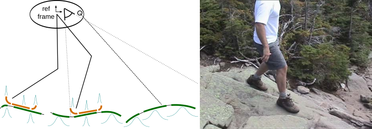
Recent advancements in control and perception have enabled bipeds to walk on flat [18] and uneven indoor terrains [99]. Major advances have also been made for outdoor quadrupeds and bipeds in rough terrain where the probability of blindly landing footholds is high [125] and uncertainty can be tolerated by low-level feedback control. Online footfall selection has been considered for quadrupeds and hexapods [75, 5, 72, 121, 60], but still, to the best of our knowledge, no physical humanoid has previously been shown to walk autonomously on unmodeled sparse 3D terrain. New advances in both perception and control [67] are required; here we attempt to disentangle these two aspects to a degree and focus primarily on perception. The foothold selection problem is particularly interesting for bipeds with non-point feet that make contact with patches of terrain. Perception is one of the key enablers for finding such patches in the environment [65, 6, 16]. This brings us to our main hypothesis (Figure 1):
Main Hypothesis: Robots operating in many unstructured environments need to perceive sparse areas for potential contact. These can be detected and modeled using curved surface patches, and spatially mapped in real-time.
1 Thesis Outline and Contributions
Sparsity of footholds for bipedal robots requires i) a model formulation for the local contact surface areas, ii) an online perception algorithm for finding them, iii) techniques for handling uncertainty and reliability, and iv) a method for creating a map of the detected local contact areas around the robot and localizing within it during motion. This thesis presents algorithms to address each of these four requirements. We have also developed and released the Surface Patch Library (SPL) [62] which contains the software implementations we used to evaluate the algorithms in our experiments.
In Chapter 2 we describe the sensing system we are using for acquiring data from the environment. This includes both a range sensor that produces a set of 3D point clouds over time and an Inertial Measurement Unit (IMU) that gives the corresponding gravity vector. We also discuss uncertainty models for the input 3D sample points associated with the sensor, along with some types of point cloud filtering, including outlier removal and smoothing. We also introduce a way for calibrating the IMU sensor with respect to the range sensor to which it is attached.
In Chapter 3 we describe the system for representing the environment. We introduce a set of 10 bounded curved-surface patch types (Figure 8 left, [160]) suitable for modeling local contact regions both in the environment and on a robot. We present minimal geometric parameterizations using the exponential map for spatial pose both in the usual 6DoF case and also for patches with revolute symmetry that have only 5DoF. We then give an algorithm to fit any patch type to 3D point samples of a surface, with quantified uncertainty both in the input points (including nonuniform variance, common in data from range sensors) and in the output patch. We also introduce an algorithm for validating the fitted patch for fit quality and fidelity to the actual data — extrapolations (like hole-filling) which are not directly supported by data are avoided ([63]).
In Chapter 4 we define the notion of a volumetric working space around the robot and we describe the patch mapping system. A dynamic map of bounded curved patches fit randomly over an environment surface that has been sampled by a range sensor is developed. The mapping algorithm is divided into four main steps after data acquisition. The first is a data pre-processing step, where both a bilateral filter is applied to the cloud to reduce noise and a sample decimation filter for performance purposes. A bio-inspired saliency filter is also introduced for detecting points in a hiking-task scenario, so only relevant parts of the environment are considered for patch fitting. Recordings of human subjects traversing rough rocky trails were analyzed to give a baseline for target surface properties for foot placement. After filtering, the second step is the selection of seed points, where a random grid-based approach is introduced and applied to the filtered samples. Next is a neighborhood search around these points. Three different approaches for finding local neighborhoods were analyzed, which have different properties near surface discontinuities. The last step is to fit the pose, curvatures, and boundary of patches to the neighborhoods and validate them to quantify fit quality and to ensure that the patch is sufficiently representative of the actual data. We finally highlight the construction of a spatial map of the fitted patches around a robot.
In Chapter 5 we present the patch tracking method that completes the whole Patch Mapping and Tracking system. For tracking the camera pose at each frame an adapted version of the Moving Volume KinectFusion [96, 132] algorithm is applied. It is the first time that this camera tracking method is used for a bipedal locomotion application on physical hardware (Kinect Fusion without the moving volume algorithm is used in [126], though in simulation only). We improve the original algorithm for our particular application both by using the gravity vector from the IMU to keep the local map in a pose aligned to gravity, and also by using a virtual camera, which lies above the robot looking down in the direction of gravity, for acquiring a point cloud from a synthetic birds-eye viewpoint during walking. In contrast to the original real camera raycasting method that considers upcoming surfaces only, the advantage of our virtual camera version is that the raycasting considers the environment around and under the robot’s feet, even portions that were previously visible but currently occluded by the robot itself.

In Chapter 6 we test the patch mapping and tracking system on a mini-biped robot platform developed in our lab called RPBP (Rapid Prototyped Biped). We ran two experiments. In the first one (Figure 2, right) we test the system integrated on the robot independently of its control, making sure that shaking and vibration while the robot is walking do not hinder the tracking process. In the second one (Figure 2, left) we first train the robot to place its foot on patches that were manually fitted on four different rocks. Then we let the robot, starting from a fixed position, detect patches in the environment and if any of them matches one of the trained patches it executes the corresponding foot placement motion. These experiments conclude the thesis, whose main contributions are as follows.
Contributions
- 1.
A new sparse environment surface representation using a set of bounded curved patches suitable for modeling local contact regions both in the environment and on the robot.
- 2.
A fast algorithm to fit these patches to 3D point samples of a surface, with quantified uncertainty both in the input points and in the output patch.
- 3.
Fast residual, coverage, and curvature patch validation tests for evaluating the fidelity of fitted patches.
- 4.
Bio-inspired rules for finding patches statistically similar to those selected by humans for hiking in rough terrain.
- 5.
Real-time mapping of hundreds of patches near a walking biped in combination with dense volumetric depth map fusion and inertial sensing.
2 Related Work
Visual odometry has been used on several current walking robots including BigDog [51, 169] and the DLR Crawler [149], though mainly for obstacle avoidance and traversability analysis, not detailed 3D foot placement or contact planning. Some steps have been made in that direction in [77], where terrain is modeled using a Gaussian Process, but this was not applied for legged locomotion.
On-line perception for foot placement has been recently implemented for quadrupeds and hexapods. In [120, 121] a continuous surface model is used for LittleDog locomotion, whereas in [8] a local decision surface was used on a hexapod walking robot. In [59, 60] a system learns optimal foothold choices from expert demonstration using terrain templates. Recently in [7] a PTAM approach was used for updating the elevation map during locomotion.
In some cases foot placement has been done without perception by using a known 3D terrain map and on-line motion capture (e.g. [24, 60]). It is also common here to use perception for obstacle avoidance, terrain categorization, or gait selection without specific 3D foot placement [169, 149]. Quadrupedal and hexapedal studies are related to the bipedal case but often use a point-like contact model, whereas many bipeds have extended feet to support torques for balance and may need to consider foot-sized terrain patches.
To date only a few works have used on-line perception for bipedal foot placement in uneven or rough terrain. In [101, 37, 38] planar segments were fitted to point cloud data for indoor scenes with slopes and steps, and in [99] a laser scanning system is used in a similar context. In [126] KinectFusion [96] was used in simulation to avoid harsh impacts. A number of other works (e.g. [83, 50, 82]) introduced perception for obstacle detection and navigation in cluttered surfaces, where the foot placement involves stepping over or climbing up/down flat obstacles. Recently [17] presented preliminary results in multi-contact planning for a full-size humanoid using 3D perception for extracting planar contact surfaces for navigation.
This thesis introduces a novel way to detect curved contact patches in the environment, whereas most prior work has focused on flat surfaces. We integrate this perception system with foot placement on rocks for a physical free-standing biped robot. Though other rough-terrain walking robots have been developed, there is little prior work in realtime on-board 3D perception for biped foot placement. Finally, our approach to map and track the patches as the robot locomotes is based on a novel combination of our sparse patch map with a dense point cloud from newly available real-time depth map fusion algorithms.
Part I Sparse Surface Modeling with Curved Patches
††margin: 2 Input Data
Both perceiving the environment around a robot (exteroceptive perception) and sensing the robot’s own internal state (proprioceptive perception) are important aspects for driving planning and control actions in a real world scenario. Various perception sensors can be used for acquiring these important measurements (see [30, 139]). In this thesis we use both exteroceptive range sensing for detecting upcoming 3D terrain contacts from a distance and proprioceptive inertial measurement unit (IMU) sensing for acquiring the robot’s orientation relative to gravity. In the next two sections we summarize the range and IMU sensors that provide the main inputs to our system.
3 Range Sensing
3D perception has gained a lot of interest over the last few years [133], mainly because low cost but high quality range sensors are now commonly available. Stereo and structured light systems, time-of-flight cameras, and laser scanners produce clouds of 3D sample points of environment surfaces in real time. Here we focus on organized point cloud data in the form of an image grid acquired from a single point of view. Initially we take such images directly from a depth camera. Then in Chapter 4 a considerable level of indirection is added: the actual depth sensor images are fused (over space and time) into a volumetric model, from which a simulated sensor extracts virtual depth images for patch mapping.

In this thesis either the Microsoft Kinect or the Primesense Carmine 1.09 (see Figure 3) have been used for acquiring 3D point clouds, depending on different experimental requirements (mainly involving range limits when the sensor is hand-held or on the mini-biped). Both the Kinect and the Carmine sensor consists of three parts: 1) an infrared (IR) projector, 2) an infrared (IR) camera, and 3) an RGB camera. For estimating the 3D point cloud a triangulation method is applied using the IR emitter and detector that are separated by a baseline. As described in [13, 68, 140, 69] in detail, given an image pixel with coordinates and disparity from triangulation, the corresponding 3D point expressed in the camera frame is:
| (1) | |||
| (2) | |||
| (3) |
using:
| image pixel coordinates and disparity of the point (in pixels) | |
| 3D point coordinates in camera frame (in physical units, e.g. m) | |
| the baseline between IR camera and projector (in physical units) | |
| IR camera focal length (in pixels) | |
| the principal point (in pixels) |
The origin of camera frame is the center of projection, the axis points into the scene through the principal point , the axis points to the right in the camera image, and the axis points down in the image. The 3D sample point coordinates in camera frame can be also expressed as a function of the coordinates of the measurement ray direction vector through pixel and the range of the data point along that vector as:
| (4) |
From the above equations, the backprojected 2D pixel corresponding to an 3D point can be calculated as:
| (5) | |||
| (6) |

Using either of these two range sensors we receive 30Hz RGB-D (red, green, blue, depth) data 11 1 Spatial registration of the depth and RGB data used built-in calibration in the range sensor (RGB data is only used for visualization purposes in this thesis).. The structured light method used by the Kinect and Carmine does not work well in full sunlight, so when outdoor data were needed they were taken at twilight. Sunlight operation could be possible with other types of depth camera or stereo vision. Two point cloud examples of rocks along with their RGB images appear in Figure 4.
3.1 3D Point Cloud Uncertainty
A big challenge with range sensors is to quantify the uncertainty of the acquired data. The uncertainty could either be due to inaccuracies in the sensor system or due to triangulation errors (i.e. the correspondence problem [137]) and it can be twofold; the data may include outlier points and noisy inliers.
Outlier Points
An outlier point is distant from the others and does not represent the underlying surface from where it was sampled. Ideally such points would be removed from the data. In many cases outliers appear along depth discontinuities due to occlusions, jumps in surfaces, or reflections. Veil points [91, 145], which are interpolated across a depth discontinuity, usually appear in data acquired by lidars (which we do not use in the thesis).
There are various methods in the literature for detecting outliers. One simple approach is to consider as inliers only the points that have a minimum number of neighbors in a fixed distance. A heuristic has been introduced in [145] for finding points that belong to borders both in foreground and background and removing those in between as veil points. Other methods, for instance the one introduced in [134], use statistical analysis for removing neighborhood points that are more than a fixed number of standard deviations away from the median. Similarly in [170] another statistical method is proposed to identify and remove outliers by checking for big residuals during plane fitting. When dealing with static environments either data fusion over time [96, 132], or outlier removal using octree raycasting as proposed in [12] can also be used.
In this thesis we address outliers both in a preprocessing step where a real-time discontinuity-preserving bilateral filter removes some outliers from the data (Section 13), and also when Kinect Fusion is used (Chapter 5) for tracking and inherently ignores some outliers when data fusion over time is applied.
Noisy Inlier Points
A noisy inlier point deviates from the ground truth that represents the underlying surface. To express the data noise we use Gaussian modeling with covariance matrices. Though this is not the only way to represent uncertainty, it does cover common situations22 2 The covariance matrices may also enable data fusion based on the Kalman filter, but in this thesis we do not explore that further.. There are various ways to estimate these covariance matrices, depending on the error model assumptions. Some assumptions can be the following (Figure 5):
- •
Constant Error (Figure 5-c): with constant nonnegative uncertainty in range, independent of the sample range, and no uncertainty in pointing direction, the covariance matrix for a sample with measurement vector is:
(7) - •
Linear Error (Figure 5-d): with a nonnegative factor that scales uncertainty linearly with the sample range, and no uncertainty in pointing direction, the covariance matrix for a sample with range and measurement vector is:
(8) - •
Quadratic Error (Figure 5-e): with a nonnegative factor that scales uncertainty quadratically with the sample range, and no uncertainty in pointing direction, the covariance matrix for a sample with range and measurement vector is:
(9) - •
Stereo Error (Figure 5-f): in Murray and Little’s [95] two-parameter error model for stereo disparity uncertainty is represented by two nonnegative parameters and :
- –
is the variance of the pointing error of the measurement vectors, represented as the variance in pixels of their intersections with the image plane at .
- –
is the variance in the disparity matching error, also measured in pixels.
The covariance matrix for a 3D point in physical units is:
(10) where:
(11) is the baseline (in physical units), the disparity (in pixels), the image pixel coordinates, and the IR camera focal length (in pixels).
- –

Whether based on stereo or time-of-flight, range data exhibits heteroskedasticity (non-uniform variance) — typically there is much more uncertainty in range than aim [110, 95], the variance changes with range, and because the measurement rays usually have a single center of projection, the error ellipsoids for the sampled points are not co-oriented: each is elongated in the direction of its own measurement ray (Fig 5).
Thus, to estimate range data covariances we apply the two-parameter pointing/disparity stereo error model proposed by Murray and Little in [95] (based on earlier work by others such as [90]) to estimate input sample covariances . The error model parameters we used for the Kinect are px, px; the former is from [74], the latter was determined experimentally following [95]33 3 For the Bumblebee2 camera and (from the specifications document).
We use this error model when fitting patches to points sampled from a single sensor viewpoint (i.e. a single captured range image). In Chapter 5 we apply KinectFusion to the range data, which provides an alternate approach to handling inlier noise by averaging over many re-samplings of the same environment surfaces. In some cases we also use either discontinuity-preserving bilateral [154] or median filters [52] to reduce noise effects:
- •
Median Filter The median filter replaces the central pixel of a fixed size window in the image with the median inside the window. The method can be very efficient [116] and effective for reducing noise and removing outliers from the data, while preserving discontinuities.
- •
Bilateral Filter The bilateral filter is similar to the median filter with the difference that central pixel’s neighbors are weighted making the filter non-linear [106].
3.2 3D Point Cloud Filtering
There are various other filtering methods for the acquired point clouds serving different purposes [133]. Some used in this thesis are the following:
- •
Passthrough: The passthrough filter removes points whose specified properties (e.g. x,y,z-coordinates, intensity, etc) are outside of some limits.
- •
Radius Outlier Removal: Removes outliers by checking the number of points in a predefined radius neighborhood.
- •
Decimation: Decimates the points by a given factor, discarding rows and columns of pixels in the image, e.g. a factor of 2 will discard all the even rows and columns.
- •
Lower Resolution: Lowers the resolution by a given factor by block averaging, e.g. a factor of 2 will replace each 2-by-2 submatrix with its average value. It is similar to the median filter, but the latter can be more robust to outliers.
- •
Voxel Grid: The approximate voxel grid filter downsamples the cloud by creating a 3D voxel grid and replacing all the points in each voxel with their centroid. This method leaves the point cloud unorganized. Some fast approximations have been introduced [133] to improve the efficiency of this filter.
4 Inertial Measurement Unit (IMU)
The use of proprioceptive Inertial Measurement Units (IMUs) for sensing the direction of gravity is very useful for locomotion. Using a CH Robotics UM6 9-DoF IMU mounted on the top of our range sensors (Figure 3), we receive 100Hz IMU data spatiotemporally coregistered with the 30Hz RGB-D data received from the depth sensor. Though an IMU can also sense velocities and accelerations, in this work we use only the gravity direction as input to our algorithms. In this thesis temporal registration of the RGB, depth, and IMU datastreams is based on timestamps, and is approximate because the underlying operating systems used were not hard real-time. Spatial registration of the RGB and depth data is based on manufacturer hardware calibration and image warping implemented in the hardware driver. Spatial registration of the depth and IMU data uses a custom calibration algorithm described next.
4.1 IMU Calibration
Calibration is required for calculating the rotation transform that gives the orientation of the UM6 relative to the range sensor. Given a dataset of depth images of a flat horizontal surface that includes a dominant plane (e.g. a flat floor) and the corresponding UM6 orientation data, the gravity vector is calculated for each depth image in the UM6 coordinate frame from the UM6 orientation data. We pair each gravity vector with the corresponding one in the depth camera coordinate frame, which is estimated as the downward facing normal of the dominant plane. For all these pairs of gravity vectors we solve the orthogonal Procrustes problem [28] that gives the UM6 to Camera transform (Figure 6).

5 Related Work
Perception and Sensing
Much research on locomotion focuses on control or path planning and assumes known terrain models or uses motion capture systems to extract information about the robot and its position with respect to the terrain (e.g. [24]). Other systems, such as [20], use only proprioceptive sensors for driving locomotion actions. For an autonomous real world task, where there is no prior information about the environment, driving actions from high-level—but quantitative—perception using exteroceptive sensors is essential. Tactile sensors are helpful only when actual contact is taking place. For a priori information about the surface, range sensing is required. There are systems that only use color cameras [33] and others that use laser scanners [99], stereo [149], or time-of-flight [130] cameras to extract depth data. Several other walking robots have used depth or RGB-D sensors, as we do, including stereo vision on QRIO [38], Xtion on NAO [83], and depth camera on HRP-2 [99, 126, 17]. Since sensors are noisy and the uncertainty of the measurements is high, perception using range sensing and IMU is a very challenging task, but it is rapidly advancing [133].
Uncertainty Representation
The importance of representing 3D range data uncertainty has been considered at least since the 80’s [90], where 2D [34] and 3D [40, 15] normal distributions were used, as well as additive zero mean Gaussian noise modeling [31] for 3D stereo measurements. In [90] non-Gaussian noise was considered for errors in the non-linear triangulation operation, which are approximated with 3D Gaussian distributions, while later in [57] a cylindrical Gaussian distribution centered at the 3D point and oriented along the measurement ray was used for modeling the stereo error uncertainty. In [23] uncertainty was modeled in the depth measurement using ellipses [42]. Tasdizen and Whitaker [150] assumed a Gaussian distribution for representing the depth noise with zero angular error. Gaussian modeling is not the only way to represent 3D point cloud uncertainty. Pauly, Mitra, and Guibas [114] considered the point cloud as a result of a stochastic process corrupted by zero-mean additive noise to come up with a likelihood and a confidence map for the data. Closed form variance formulations [3] and non-Gaussian distributions [105] are also alternative ways to represent the uncertainty of the range data. Recently an uncertainty model for the Kinect sensor has been introduced [68, 140, 69], while a mixture of Gaussians has been used in [25].
6 Summary and Future Work
In this chapter we introduced the input data acquisition process for both exteroceptive (range sensor) and proprioceptive (IMU sensor) data. We discussed error modeling for the range data and different types of filtering for 3D point clouds. We also described a method for calibrating the IMU sensor with respect to the RGB-D camera on which it is mounted.
Data fusion is a key aspect in robotics and has been studied exhaustively. An interesting direction for bipedal locomotion perception is to fuse exteroceptive (range sensing) and proprioceptive (kinematics and tactile sensing) data for detecting contact areas in the environment. Exteroception can detect upcoming terrain contact areas from a distance, but with relatively high uncertainty. Kinematic proprioception senses the pose of contact areas on the robot itself—e.g. heel, toe, foot sole—potentially with relatively low uncertainty. Once a contact is established, the environment contact area can be re-measured exproprioceptively through kinematics and touch, possibly with reduced uncertainty compared to prior exteroception. Finally, the uncertainty representation plays an important role in 3D perception. Various ways of modeling uncertainty have been introduced, but there is not yet a generally accepted model and further investigation is needed.
††margin: 3 Environment Representation
Some of the most challenging open problems in robotics are those which require reliable contact with unstructured world surfaces when locomoting (Figure 7 right). To enable rough-terrain walking and climbing, a perception system that can spatially model and finely quantify potential 3D contact patches may be needed. Contact is well-studied (e.g. [89]) but, arguably, there is not yet any accepted general system for modeling the shape and pose of potential contact surface patches, including both patches on the robot (e.g. finger tips, foot soles, etc) and also in the surrounding environment. This is especially true when (a) curved, bounded patches with (b) geometrically meaningful minimal parameterizations and (c) quantified uncertainty are desired (Figure 7 left).
Why curved patches? Our interest is legged locomotion on large rocks. Flat areas can be rare in such natural environments. More broadly, contact surfaces in man-made environments are also often curved—railings, doorknobs, steering wheels, knobs, etc. Though curved surfaces can be approximated by sets of smaller planar patches [157], the job can often be done with fewer and larger curved patches. Curved surface geometry is more complex, but it may still be an advantageous trade-off to reason about fewer and larger patches. For example, a spherical robot foot stepping into a divot on a rock might be modeled as the interaction between just one spherical and one elliptic paraboloid patch (on foot and rock, respectively). If the surfaces were approximated using collections of smaller planar patches the interaction could require combinatorial reasoning about many possible contacting pairs.
By “geometrically meaningful minimal parameterizations” we mean that each patch is defined by the fewest possible parameters, and that these have direct geometric interpretations—rotations, translations, curvatures, lengths, and angles. Geometric (vs. algebraic) parameterizations also support reasoning [22] about possible actions with patches, and allow some representation of spatial uncertainty with geometric error ellipsoids. Minimality is desirable because redundant (non-minimal) parameterizations can slow the numerical optimizations used in surface fitting [36] and must be handled specially in uncertainty modeling [110].
It is often important to get both a best estimate of patch parameters and a quantification of the uncertainty therein. We develop full uncertainty quantifications based on Gaussian modeling with covariance matrices as were described in Chapter 2, by propagating the input 3D point cloud uncertainty [92, 153] to the output patch. Though in this thesis we use dense volumetric depth map fusion for mapping (Chapter 4), we also intend our models to be usable in sparse Kalman-type SLAM (Simultaneous Localization and Mapping [142, 141, 26]) algorithms that maintain a dynamic local patch map, Figure 7, of contact patch features around a robot. Such a map could potentially include both environment surfaces and contact pads on the robot itself, which may themselves be potentially uncertain due to kinematic error.
We first give the details of the patch models for representing the environment in local contact areas, followed by an algorithm to fit and validate a patch to noisy point cloud data from common types of range sensor. This fitting is the main step in using patches to represent surface shape and pose. We also demonstrate the algorithms in experiments with simulated and real range data. More experiments are presented in Chapters 4 and 6 in practical contexts including humans walking on rocky natural terrain and a biped robot walking near and stepping on rocks.
7 Patch Modeling
In [160], we introduced a general-purpose set of ten curved and flat patch types (Figure 8, Table 1) suitable for both natural and man-made surfaces and balancing expressiveness with compactness of representation. Eight come from the general second-order polynomial approximation to a smooth surface at a given point—the principal quadric—which is always a paraboloid, possibly degenerated to a plane [118]. We add two non-paraboloid types to better model common man-made spherical and cylindrical surfaces, and we pair each surface type with a specific boundary curve to capture useful symmetries and asymmetries. Each patch is parametrized using extrinsic and intrinsic parameters (see parametric surfaces in [94]) for its shape and spatial pose.

| surface | bound | parameters | DoF | world frame equations | |
|---|---|---|---|---|---|
| intrin. | extrin. | ||||
| elliptic paraboloid | ellipse | 10 | (26,27,29); | ||
| hyperbolic paraboloid | ellipse | 10 | (26,27,29); | ||
| cylindric paraboloid | aa rect | 9 | (26,27,30,31); | ||
| circular paraboloid | circle | 7 | (26,27,29); , | ||
| plane | ellipse | 8 | (26,27,29); | ||
| circle | 6 | (26,27,29); , | |||
| aa rect | 8 | (26,27,30,31); | |||
| c quad | 11 | (26,27,33,31); | |||
| sphere | circle | 7 | (36,37,29); , | ||
| circular cylinder | aa rect | 9 | (40,41,30,31); | ||
7.1 Extrinsic and Intrinsic Surface Parameters
An instance of a patch will be a vector of real parameters which define both its shape (curvature and boundary) and its 3D rigid-body pose. We call the former intrinsic and the latter extrinsic parameters [143]. We must consider different issues to achieve minimal parametrization for each, and the distinction also enables the option to model shape (intrinsic) and pose (extrinsic) uncertainty separately. Minimal intrinsic parametrization for the proposed patches will be given by (a) one parameter for each variable curvature, and (b) a minimal parametrization of the boundary curve. However, minimal extrinsic parametrization depends on the continuous symmetry class of the patch. For example, a patch with two different curvatures (Figure 9 left) has no continuous symmetry: its rigid body pose—here any element in the special Euclidean group —has six degrees of freedom (DoF).
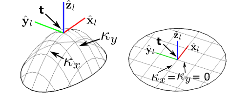
But a planar patch with a circular boundary (Figure 9 right) has a continuous rotation symmetry and only five extrinsic DoF. Remarkably, it has been shown that there are exactly seven continuous symmetry classes in 3D [143]: revolute, prismatic, planar, spherical, cylindrical, helical, and general (the first six correspond to the lower kinematic pairs; the last represents no continuous symmetry). Since we only consider patches with boundaries, we need only the general (no continuous symmetry, 6 DoF pose) and revolute (one continuous rotation symmetry, 5 DoF pose) classes—continuous translation symmetries are not possible for bounded patches.
7.2 Pose Representation with the Exponential Map
We require two extrinsic parameterizations: one with six parameters for asymmetric patches and one with five parameters for patches with revolute symmetry. It is well known that, because the Lie-manifold of the special orthogonal group (the rotation subgroup of ) is non-Euclidean, there is no singularity-free minimal parametrization of . For the general 6-DoF case we thus select a minimal parametrization with singularities that are easiest to handle for our application. One of the core computations will be patch fitting by iterative optimization, and for this Grassia showed in [36] that a useful pose representation is44 4 We explicitly notate transposes; orientation is crucial esp. for Jacobians.
| (12) |
where is a translation and is an orientation vector giving an element of via an exponential map. Grassia observed that in this parametrization singularities are avoidable by a fast dynamic reparameterization, reviewed below.
We use Rodrigues’ rotation formula for the exponential map (Grassia used quaternions):
| (13) | |||
Despite division by , (13) converges to as . For numerical stability we use the series expansion approximations and for small (e.g. for ). As promised, the representation has a direct geometric interpretation: is just a translation, and (wlog for ) gives the right-hand-rule rotation angle about the spatial axis defined by the unit vector . While exponential map approaches are not new [14, 107], matrices in , the Lie algebra of , are typically used instead of . Though elegant, the former do not satisfy our goals of minimal parametrization and direct geometric interpretation.55 5 It is true that there is a 1:1 correspondence between matrices in and elements of the parametrization; conceptually, we have invoked this correspondence and simplified the results directly in terms of .
Using the fact that counterclockwise rotation by is equivalent to clockwise rotation by , Grassia’s reparametrization converts any into a canonical 66 6 For there is still ambiguity between and ; this can be resolved by a consistent sign policy. one with :
| (14) |
represents the same rotation as , but stays away from the singularity surfaces where is a multiple of .
Algebraically, corresponds to an element
of , a homogeneous rigid body transform, and can thus define the pose of a local coordinate frame (and a patch therein) relative to a world frame : is a basis for and is its origin. The transformation of a point in to in , and the reverse, are familiar functions
| (15) | ||||
| (16) |
where (16) makes use of the inverse transform
| (17) |
Equations (12–16) constitute our 6 DoF pose parametrization. For the 5 DoF case, observe that only one of the three basis vectors of need be specified; rotation symmetry allows the others to make any mutually orthogonal triple. Only two DoF are required, equivalent to specifying a point on the unit sphere. We do this by re-using (12–16) with fixed at 0:
| (18) |
The geometric interpretation of is the same as for , except that is constrained to the plane. In some contexts we may want to calculate an that induces a local coordinate frame with the same as a given . For any given canonical , a canonical always exists that satisfies
| (19) |
can be calculated as
| (20) | |||
As in Brockett’s product of exponentials [14], 6 DoF poses can be composed to make any kinematic chain. Let
| (21) |
be the poses (equiv. transforms) in the chain from end to base in order from right to left. Then the pose of a patch attached to the end of the chain relative to the base is
| (22) | |||
substituting for 5 DoF patches, and using the log map corresponding to the inverse of (13). We give an algorithm to compute in Appendix 8.B.
7.3 Patch Models
We now present the details of ten surface patch models (Figure 8, Table 1) based on seven curved surface types. Five of these partition the paraboloids, including the important degenerate case of a plane; the other two add true spherical and circular cylinder patches, non-paraboloids that are common in man-made environments and on robots. For non-planar surfaces we select one specific parametrized boundary shape which trims the surface into a local patch. For planes we allow a choice of four boundary shapes.
The next two sections give the details of the paraboloid and non-paraboloid patch models. This particular system is not the only possible taxonomy; it reflects our design choices in an attempt to balance expressiveness vs minimality.
7.3.1 Paraboloids
The best-fit degree-two local polynomial approximation to any smooth surface at a given point , called the principal quadric, is always a paraboloid—a quadric of one sheet with a central point of symmetry about which the surface has two independent curvatures in orthogonal directions (Figure 9 left). These are the principal curvatures of at , and is the symmetry point. Defining and as unit vectors in the directions of the principal curvatures in the tangent plane to at , the surface normal to at is . If is considered to be embedded in a world coordinate frame , then is the origin and
is a basis for the principal coordinate frame (all standard terms) of at , which we also call local frame 77 7 L is also the Darboux frame [41] of the paraboloid.
Using the log map, the transform
takes points from to , enabling a short derivation of equations for a general paraboloid parametrized by , , and . Starting in where the paraboloid is in standard position, with and ,
| (24) | ||||
| (25) |
are the implicit and explicit forms for the surface equation, respectively, with a point on the patch in and parameters of the explicit form. Moving to in world frame is accomplished by composing (24,25) with (15,16), yielding
| (26) | ||||
| (27) |
Note that in this formulation is always the projection of onto the local frame plane:
| (28) |
In the general case , giving 7 or 8 DoF paraboloids—6 pose DoF plus up to two curvatures (boundary parameterizations will add DoF). Six DoF pose is required because implies no continuous rotation symmetries, only discrete symmetries about . It is standard to separate three surface types where (Figure 8): elliptic paraboloids have two nonzero curvatures with equal signs, hyperbolic paraboloids have two nonzero curvatures with opposite signs, and cylindric paraboloids have one nonzero curvature. In all cases is the outward pointing surface normal and positive/negative curvatures correspond to concave/convex directions on the patch, respectively88 8 To reduce ambiguity wlog choose , though some ambiguity is unavoidable due to bilateral symmetries..
Boundaries

We bound elliptic and hyperbolic paraboloid patches with ellipses in the plane of the local frame , axis aligned and centered at (Figure 10 (b)). If are the ellipse radii then the bounded patch is the subset of the full surface (24–27) where, with , satisfies
| (29) |
For cylindric paraboloid patches, replace the ellipse boundary with an axis aligned rectangle with half-widths (Figure 10 (a)). In the plane of the vertices are
| (30) |
in counterclockwise order, and the bounding condition can be stated as, with ,
| (31) | |||
where is the implicit form for a 2D line given two points on the line; is on or to the left of the directed line through towards iff
| (32) |
For the special case we identify two more surface types (Figure 8): circular paraboloids have both curvatures equal and non-zero, and planes have both curvatures zero. Both of these have continuous rotation symmetry about , so we use the 5-DoF pose parametrization , provided that the patch boundary also has the same continuous rotation symmetry. The latter holds for circular boundaries, which we use for circular paraboloids (Figure 10 (d)). Let be the surface curvature and the bounding circle radius; circular paraboloids are then defined by (24–29) with , , , and with the dimensions of the function domains correspondingly reduced.
For the important case of paraboloids degenerated to planes we give a choice of four boundary types: ellipses, circles, rectangles, or general convex quadrilaterals (developed next). For all except circles, the planar patch loses its continuous rotation symmetry and requires full 6-DoF pose parametrization; the patch is defined by (24–27) with (and correspondingly reduced function domains) and either (29) or (31). Planar patches with circular boundary are the same as circular paraboloids but with .
For convex quadrilateral boundaries, keep at the intersection of the diagonals and (Figure 10 (c)), where are the vertices in counterclockwise order in the plane of local frame . Define as half the angle between the diagonals and the half-diagonal lengths such that
| (33) | |||
Then the quadrilateral is defined by (31) using vertices (33) parametrized by . Convexity is ensured by construction, and only five parameters are needed even though a general planar quadrilateral has 8 DoF—the remaining three (a rotation about the plane normal and two in-plane translations) are contributed by the extrinsic pose.
7.3.2 Spheres and Circular Cylinders
Spheres and circular cylinders are common on robots and in man-made environments. Though still quadrics, neither is a paraboloid, suggesting two additional patch types (Figure 8). (We do not model complete spheres or cylinders, only bounded patches of hemispheres and half-cylinders.)
Again starting in local frame , the implicit and explicit equations of an upright hemisphere with apex at the origin and curvature (hence possibly infinite radius ) are99 9 In the limit as (34–41) all reduce to planes., with and ,
| (34) | ||||
| (35) |
Composing these with (15,16) gives the world frame forms ,
| (36) | ||||
| (37) |
Circular half-cylinder surfaces are similar but (a) have no dependence on and (b) require 6 DoF pose:
| (38) | |||
| (39) | |||
| (40) | |||
| (41) |
Boundaries
8 Patch Fitting
Having defined the patch models, it is natural to consider recovering contact surface areas in the environment by fitting bounded curved patches to noisy point samples with quantified uncertainty both in the inputs (the points) and the outputs (the patch parameters), which is not a trivial problem1010 10 We have found very few prior reports on the particular fitting problem including boundaries and quantified uncertainty. (Figure 11). Though linear least squares (LLS) can fit a quadric surface to points [22], and its extension to linear maximum likelihood fits data corrupted by white noise, the problem appears to become non-linear when the points are heteroskedastic (i.e. have nonuniform variance). Also, we want to fit bounded paraboloids, spheres, and circular cylinders, not just unconstrained quadrics.

In [160] we give a non-linear fitting algorithm which handles these issues. It is based on a variation of Levenberg-Marquardt iteration that fits a bounded curved patch to a set of 3D sample points. The algorithm minimizes a sum-of-squares residual by optimizing the patch implicit and explicit parameters. The residual for an individual sample point is computed by scaling the value of the implicit form by the inverse of a first-order estimate of its standard deviation, which is derived in turn from a covariance matrix modeling the sensor uncertainty for the point.
Next we describe the patch fitting algorithm. Elliptic, hyperbolic, circular, and cylindrical paraboloid as well as planar patches are fitted automatically depending on the detected curvatures of the underlying surface. The non-paraboloids (cylindrical and spherical patches) are fitted only if requested. Also, similarly, for planar paraboloids, the type selection for the boundary curve is only partially automatic — rectangles and convex quads are only used if requested.
8.1 Patch Fitting Algorithm
The inputs are (Figure 12):
- •
sample points with covariance matrices (positive semi-definite)
- •
the general surface type to fit1111 11 Taking as inputs allows constrained fitting of specific types; they could be automatically found by checking all possibilities for the best fit. {parab, plane, sphere, ccyl}
- •
the boundary type {ellipse, circle, aarect, cquad} if 1212 12 is implied if .
- •
a boundary containment probability

The outputs are:
- •
the fitted patch type
- •
parameters , where is the DoF of the patch type (Table 1)
- •
covariance matrix

The algorithm proceeds in 2 stages (9 total steps), which include heuristics for avoiding local minima when solving the non-linear system. The first three steps fit an unbounded surface; the rest are largely concerned with fitting the boundaries, which can include final resolution of the patch center and orientation (in steps 6 and 9) where the bounding shape breaks symmetries of the underlying surface. An illustration of the whole fitting process for a simulated paraboloid can be shown in Figure 13.
- Stage I:
Fit an Unbounded Surface
- Step 1:
Plane fitting
- (i)
Fit a plane with LLS, ignoring .
- (ii)
Unless , re-fit the plane with weighted Levenberg-Marquardt (WLM), detailed below, including , using (36) with .
- (iii)
Set (perp. proj. of on plane).
Note that:
- •
At the end of Step 1 the refined plane is defined by (i) the point on it, which is the centroid of the data and (ii) by the plane normal which is the third column of the rotation matrix. Note that the third element of the rotation vector is zero, since it is currently a 2D orientation vector, because an unbounded plane is rotationally symmetric about its normal. Note also that an unbounded plane has only 3-DoF, not 5-DoF. The extra two DoF are constrained during fitting by keeping at the projection of the centroid of the data points onto the plane. There is a choice of boundary shapes for plane fitting, and all except circular will break the rotational symmetry of the unbounded plane. This is handled later in Step 9, where it may be necessary to extend the rotation vector from 2D to 3D.
- •
(if ): Since a general assymetric paraboloid will be fitted by WLM in Step 2, probably a relatively expensive WLM in Step 1 will not improve the refinement. The plane fit by LLS in Step 1-i will serve to initialize WLM to the correct region of parameter space (which is important, because WLM will only find a local optimum), but all components of and (the only parameters we have estimated so far) will be replaced by the WLM in Step 2.
- •
(if ): Since the end goal is to fit a plane and there will be no WLM in Step 2 for planes, it is required to refine it in Step 1-ii, and importantly, to get its covariance matrix. Note that in Step 1-ii a redundant parameterization is used, since the point on the plane (defined by ) has two extra DoF to slide around on the plane. This redundancy is compensated by constantly adjusting at the projection of the data centroid onto the plane (a point that is well centered in the data is preferable, since all the planar patch boundary shapes (ellipse, circle, aa rect, convex quad) are origin-centered).
- •
(if ): Since in this case the end goal is a spherical patch, and in Step 2 only an unbounded (i.e. complete) sphere will be fitted, there is a need to extract the orientation of the patch, which is not coming from the WLM. It is determined, instead, by the plane normal calculated here in Step 1. Thus the plane normal estimation is essential, including the uncertainty of the input data points. The LLS in Step 1-i did not consider that uncertainty, so it is needed to refine the plane fit with WLM.
- •
(if ): For circular cylindrical patch, the logic is similar to the spherical patch. The WLM in Step 2 fits an unbounded cylinder and the orientation of the final bounded cylindrical patch will come from a combination of the plane normal that is calculated here and the direction of the cylinder symmetry axis recovered in the WLM in Step 2.
- (i)
- Step 2:
- Step 3:
Curvature Discrimination (if )
- Step 1:
- Stage II:
Fit the Boundary
Having fitted an unbounded patch to the 3D data, the boundary needs to be determined. Principal Component Analysis (PCA) is applied to the 2D projected points onto the local -plane for finding the enclosing boundary. A closed-form solution [129] for the corresponding eigendecomposition problem using 1D and 2D moments to fit approximate boundaries is used. Note that the difference between planar and non-planar patches is that for the latter the principal direction axes are the axes of the local reference frame (implied by the principal curvatures of the underlying surface), whereas for the planar patches the axes need to be determined by fitting the boundary shape.- Step 4:
Determine the Boundary Type (if )
Set based on . If the patch is not a plane then the type of the boundary is uniquely defined from the type of the patch (Table 1). Otherwise it is determined from the user as an input.
Set for boundary containment scaling [127].
- Step 5:
Initialize Bounding Parameters
Project the data to using (28).
Set first and second data moments: , , , .
- Step 6:
Cylindrical Paraboloid and Circular Cylinder Boundary Fitting
If set and , where is the standar deviation along the axis of the local frame and is the standard deviation along the axis (the data are already zero-mean in due to the nonzero principal curvature in that direction).
- Step 7:
Circular Paraboloid and Sphere Boundary Fitting
If set .
- Step 8:
Elliptic and Hyperbolic Boundary Fitting
If set .
- Step 9:
Plane Boundary Fitting
- (i)
If , and will be available from either 1 or 3. The extents and rotation of the boundary curve are determined now by two-dimensional PCA.
Set and (c.f. [129])
(42) - (ii)
If set and from using (20).
- (iii)
If set .
- (iv)
If set1313 13 We currently fit convex quad the same as aa rect, but note that the former is still useful for designed (vs fit) patches, e.g. part of a foot sole.
(43) - (v)
If , determine the in-plane rotation of the boundary shape by setting
(44)
- (i)
- Step 4:
The fitting process for all types of curved bounded patch models is illustrated in Figure 14. The covariance matrix of the patch parameters is calculated by first order error propagation through the above computations in each step (see Appendix 8.C).

8.2 The side-wall effect problem and flipping patch normals towards viewpoint
When the neighborhood points don’t have a central symmetry then they may be unevenly distributed in the patch if left unconstrained. We call this the side-wall effect (Fig. 15). To handle this, in [63] we introduced a constrained fitting where the center of the patch must lie on the line through the centroid of the neighborhood parallel to the normal to an initial fit plane. This is implemented as a reparameterization during the WLM incorporated in Step 2
| (45) |
where is the new patch parameter replacing . Note that this constrained fitting affects the error propagation (see Appendix 8.C).

The “outward” facing direction of the patch surface normal, which is the same as the local frame basis vector , is ambiguous globally in the point cloud. But considering that the the data were acquired from a single point of view then the following equation should be satisfied:
| (46) |
If not we flip the patch by rotating it’s local frame basis around and flipping its curvatures.
8.3 Weighted Levenberg-Marquardt
Levenberg-Marquardt (LM) is a standard iterative non-linear optimization [124]. It can find a parameter assignment that locally minimizes the sum-of-squares residual of a differentiable objective function applied to a dataset , , starting from an initial estimate . That is, it finds
| (47) |
Implementations typically take as inputs functions and , the data , and , and return both and a covariance matrix representing its uncertainty. A well known extension is to replace with where are constant standard deviations modeling uncertainty in . The residual is then called , and locally maximizes the likelihood of the “observations” .
For our use, is always the implicit form of a surface in world frame, i.e. , , or (26,36,40). The are not constant, but can be estimated with with first order error propagation as1414 14 This assumes the ’s are positive-definite, which is a common requirement for covariance matrices. A heuristic to allow semi-definite is to clamp small to a minimum positive limit.
| (48) | |||
We define weighted LM (WLM) to combine and into a meta-objective function :
| (49) |
Both and its gradient are implied given , , , , , and (which is ):
| (50) |
Given , , , , , and , WLM synthesizes and by (49,50) and then applies LM. This is simplified further by the common implicit form of the world-frame surfaces (26,36,40), which are all variants of
| (51) | |||
| (52) | |||
where some components of , and for (36) the last component of , are held at zero. The required derivatives of (52) are given by the chain rule from (23) and derivatives of (51) (using ):
| (53) |
| (54) |
| (55) |
8.4 Experimental Results
We tested the fitting algorithm both in real data from a Kinect viewing a rock and in simulation (Figure 11). For this initial experiment we implemented a simple interactive segmenter to manually select neighborhoods to fit patches in the 3D point cloud of the rock. In Chapter 4 we present algorithms for automatic neighborhood finding. We used the two-parameter pointing/disparity stereo error model proposed by Murray and Little in [95] to estimate input sample covariances for all experiments (as described in Chapter 2).
The results show that the algorithm can produce reasonable curved-surface patch models for local parts of non-flat environment surfaces. Average times for our Matlab implementation are 20ms to fit sample points on a commodity workstation, while in a implementation we reached 0.6ms to fit sample points. SVD computations within LM are quadratic in , though runtime also depends on the LM convergence rate.
Note: In the rest of this thesis we will consider fitting only paraboloid patches, unless otherwise indicated. Paraboloids are complete in that they form an approximation system for local regions on any surface with zero,one, or two nonzero local principal curvatures.
9 Patch Validation
After fitting a patch to a set of point cloud data it is important to evaluate it, because it may fit the data but still not faithfully represent the surface. In [63] we introduced three measures based on the residual, coverage, and curvature. Residual and curvature evaluate the surface shape, while coverage evaluates the boundary of the patch. (see Figure 16).

9.1 Residual Evaluation

The patch residual measures the deviation between the sample points and the (unbounded) patch surface. The residual can be bad either due to outliers (see Figure 17) or due to local minima in the WLM process. We use the root-mean-square error (RMSE) Euclidean residual between the sample points and their corresponding closest points on the patch1515 15 Here we consider both and to be expressed in the patch local frame . (which must be calculated for each )
| (56) |
Whereas the patch fitting algorithm uses an algebraic residual for speed, is a Euclidean residual and gives its result in the same physical units as the input data (e.g. meters) [122], enabling it to be compared to a meaningful threshold. However, calculating the for each can be computationally expensive. We use a technique based on Lagrange multipliers [27].
When the paraboloid surface was fitted as a plane, so , i.e. is the projection of onto the plane of . Otherwise is characterized as:
| (57) |
Define a Lagrange function as
| (58) |
with Lagrange gradient constraints
| (59) |
Expand the first gradient constraint from (59)
| (60) |
and substitute1616 16 The inverse of the diagonal matrix in (60) is evaluated symbolically and then denominators are cleared after substitution in (51), avoiding any issue of non-invertability or division by zero. for in the second gradient constraint, which is the same as (51).
This leads to a fifth degree polynomial in , for which there is at least one real solution because imaginary solutions come in pairs. To solve the polynomial, we can either compute the eigenvalues of the companion matrix or we use Newton iteration. For Newton’s method an initial root guess for (and thus for ) is required. We pick as the point projected from along the -axis (local frame). Newton’s method appears to be times faster than Eigendecomposition in tests with around sample points per patch.
Finally, backsubstitute1717 17 Division by zero can occur during this backsubstitution when is on a symmetry plane or axis, but alternate forms can be used in those cases. the real solution(s) in (60) and find the minimum as in (57).
Residual Approximations

The problem of the Euclidean residual estimation is well studied, both for exact and approximate solutions; for instance Taubin’s first and second order approximations [151, 152], the 3L algorithm [11], the constrained minimization method [1], and MinMax [43] have been proposed.
We implemented three approximations. The simplest approximation is to consider the vertical distance in the local -axis of the patch. The other two are the first and second order Taubin approximations introduced in [152] (see Appendix 8.D). We tested these approximations in simulated data. For each patch type we sampled a set of point data (a range of 60-200 points per patch) and we perturbed them in the direction of the surface normal at each point (Figure 18). All the approximations are times faster than the exact solution of solving the fifth degree polynomial. Both Taubin’s approximations are very close to the exact solution, compared to the vertical distance one that does not give good results at all.
Residual Thresholds
To determine the residual threshold such that any patch with will be dropped, we sorted all residuals (Figure 19) for a sampling of 1000 random patches (m, k-d tree neighborhoods), 100 on each of 10 rock datasets [63]. The value m was selected to include approximately of the patches. In general can be set in an application dependent way. Furthermore, the choice of RMSE residual is not essential. For example, an alternate residual
| (61) |
could be used to check if any small surface bumps protrude more than a desired amount from the surface.

9.2 Coverage Evaluation

A different evaluation is needed to take into account the patch boundary. A patch may fit the data but still not faithfully represent the neighborhood, either because too many sample points are outside the patch boundary or there is too much area inside the boundary that is not supported by data points. (Unlike [73], we opt not to speculatively fill holes in the data.)
To detect these cases we generate an axis-aligned grid of fixed pitch on the plane of the patch local frame . We generate only the required number of rows and columns in this grid to fit the projection of the patch boundary.
Define and to be the number of data points whose projections are both inside a given cell and respectively inside or outside the projected patch boundary. Define to be the area of the geometric intersection of the cell and the projected patch boundary, which will be detailed below. The cell is considered bad iff
| (62) |
for thresholds and . Here we fix these thresholds relative to the expected number of samples in a given cell if all samples were in-bounds and evenly distributed:
| (63) |
where is the number of sample points in the neighborhood and is the area of the patch approximated as the area inside the projected boundary.
The patch fails coverage evaluation iff there are more than bad cells. After some experiments in fitting paraboloid patches with neighborhood radius m, we set m, , , and . Figure 20 illustrates patches that pass and fail coverage evaluation.

Intersection Area for Ellipse and Circle Boundaries
For an ellipse boundary with radii , or for the degenerate case of a circle boundary with radius , we compute the intersection area with a secant approximation since the exact computation involves a relatively expensive inverse trig function. Wlog we describe only the top right quadrant (Fig. 21, left); the other three are symmetric. Let be the four corners of a grid cell in counter-clockwise order starting from the lower left. The algorithm for computing the intersection area is:
- 1.
If is inside the ellipse then
- 2.
else if is not inside the ellipse then
- 3.
else if is inside the ellipse then
if is inside the ellipse then else - 4.
else if is inside the ellipse then
- 5.
else .
| (64) | ||||
| (65) | ||||
| (66) | ||||
| (67) |
Intersection Area for Axis-Aligned Rectangle Boundary
As above we consider only the top right quadrant (Fig 21, middle). Let the rectangle half-lengths be , and define . The exact intersection area can be computed as follows:
- 1.
If is inside the rect then
- 2.
else if is not inside the rect then
- 3.
else if is inside the rect then
- 4.
else if is inside the rect then
- 5.
else .
Intersection Area for Convex Quadrilateral Boundary
To handle the case of a general convex quadrilateral (Fig. 21, right), we use the fact that the intersection between a convex quad and a rectangle is always convex:
- 1.
Find the set of grid cell corner points that are inside the quad and vice-versa.
- 2.
Find the intersection points between the grid cell boundaries and the convex quad boundaries.
- 3.
Discard all points from steps 1 and 2 except those that lie in or on both figures.
- 4.
Sort all the points computed in the previous steps in counterclockwise order and connect the first point with each of the others in order, forming a triangle fan. is the sum of the triangle areas.
9.3 Curvature Evaluation
Residual and coverage evaluation may still not be enough. There may be cases where both residual and coverage checking passes, but the bounded patch does not represent the data correctly. This may happen either when the point cloud data form a very curved surface or when the the LM non-linear fitting gets stuck in local minima as appears in Figure 22 in yellow. A patch fails curvature evaluation iff its minimum curvature is smaller than a threshold or its maximum curvature is bigger than a threshold . We set this threshold experimentally to and , where is the patch boundary vector.

More fitting and validation experimental results are presented in Section 18.
10 Related Work
Modeling
Modeling the environment and detecting potential contact surface areas around a robot using exteroceptive sensing is a common task, but still very challenging, especially for locomotion in uncertain environments. The approach explored here contrasts with the traditional study of range image segmentation, which also has a significant history [47], where a partition of non-overlapping but potentially irregularly bounded regions is generated producing a dense labeling of the whole image. In image segmentation, some work has been done with curved surfaces [123], but the main focus still appears to be on planes [56, 164, 38, 110].
Many prior systems typically use dense approaches in that they attempt to model all of the terrain in view. Some are grid based [4], like those on Ambler [75], Dante II [5], and Mars Exploration Rovers (MER) [84] using laser scanners or stereo cameras to build an elevation map, find obstacles, and quantify traversability. Usually these don’t model detailed 3D contact features, though some attempt to recover surface models [121]. A few other works do take a sparse approach but are restricted to planar patches, ranging from large flats in man-made environments [164, 38, 110] down to small “patchlets” [95].
We proposed to only map a sparse set of patches. Also, our patch-based approach can homogeneously model contact surfaces both in the environment and on the robot itself, whereas most prior work considers modeling environment surfaces exclusively. Irregularly bounded regions, which may be very large or non-convex, can present a challenge for higher-level contact planning algorithms which still need to search for specific contact areas within each region. One aim of using regularly bounded regions of approximately the same size as relevant contact features on the robot is to trade potentially complex continuous searches within patches for a discrete search across patches. Fewer and larger paraboloid patches can give a comparable fidelity of representation as the many small planar patches needed to cover a curved environment surface [157]. Of course other parts of the robot may also make contact in unintended ways. The patch model could help plan intentional contacts while other data structures are simultaneously used for general collision prediction [144, 117, 17, 50].
One challenge in modeling is dealing with missing data. In [72] texture synthesis was presented to deal with the problem of occluded terrain by filling in the missing portions. Our approach avoids representing such missing areas where uncertainty is high. As we described in Chapter 5 we instead integrate multiple range scans taken from different perspectives (as the robot moves) to fill in missing areas with new observations using a volumetric fusion approach [96, 132].
Fitting
One of our main results [160] is an algorithm to fit curved, bounded patches to noisy point samples. Fitting planes is well studied [161], including uncertainty [61] and fitting heteroskedastic range data [110]. For curved surfaces quadrics are a natural option; Petitjean [118] surveyed quadric fitting, but there were few results that (a) quantified uncertainty, (b) recovered geometric parameterizations, and (c) fit bounded patches. In [22], Dai, Newman, and Cao describe recovery of paraboloid geometric parameters1818 18 They verify that the fit result is a paraboloid and extract its parameters. They do not consider constraining the fit to paraboloids (vs other quadrics). by linear least squares, without considering uncertainty. In [162] Wang, Houkes, Jia, Zhenga, and Li studied quadric extraction in the context of range image segmentation, including quantified uncertainty in the algebraic (not geometric) patch parameters, but not on the input points, while in [165] superquadrics are fit using Levenberg-Marquardt considering variance in the range data. Our fitting algorithm quantifies both input and output uncertainty and recovers geometric parameters of bounded patches.
11 Summary and Future Work
We introduced a set of 10 particular bounded curved-surface patch types and algorithms to fit and validate patches to noisy point samples of a surface for sparsely representing contact surfaces in the environment near a robot, and also on the robot itself. Paraboloid (including planar) patches can model portions of natural surfaces such as rocks; planar, cylindrical, and spherical patches can model common types of man-made surfaces as well as portions of the robot feet and hands. The presented patch models all have minimal geometric parameterizations and quantified uncertainty in the form of covariance matrices. Though surface modeling and surface fitting have been studied extensively, many prior works ignore uncertainty, are limited to planes, are dense vs sparse, and/or are concerned only with surfaces in the environment. We address all of these issues to some extent and we demonstrated the effectiveness of our approach both in real data and in realistic simulation.
Fast patch fitting is a key aspect of the proposed method. The presented algorithms are efficient enough for our application in bipedal locomotion (Section 8.4, Section 18, and Chapter 6), but it is of great interest to check weather a fast normal vector and/or principal curvature extraction (e.g. using Integral Images [46]) can replace the initial parameter estimation during WLM and reduce the number of iterations. Moreover, a re-fitting process could be developed where an initially fitted patch (coming for instance from a previous frame) is refit to new data. Validation and visualization of the covariance matrices of the patch parameters calculated by uncertainty propagation (Appendix 8.C) is another possible next step for this work. Finally, an extension to higher degree polynomials could be added for representing more irregular areas in the environment, while preserving geometrically meaningful minimal parametrization and quantified uncertainty.
Part II Curved Patch Mapping & Tracking
††margin: 4 Patch Mapping
Having introduced in Chapter 3 a new surface model for contact patches between a robot and local areas in the environment and algorithms to fit and validate patches to 3D point cloud data, algorithms to find potentially useful patches and spatially map them relative to the robot are now presented. Patches are sparsely fit using the following five-stage approach1919 19 Though we describe each stage as a batch operation, in practice the implementation of Stages III to V is “pipelines” so that patches can be added to the map incrementally until a time or space limit is reached. (Figure 23):
- Stage I:
Acquire Input Data from a Depth Camera and IMU (Section 12).
- Stage II:
Preprocess the Input Point Cloud (Section 13).
- Stage III:
Select Seed Points on the Surface (Section 14).
- Stage IV:
Find Neighborhoods of Seed Points (Section 15).
- Stage V:
Fit & Validate Curved Bounded Patches to the Neighborhoods (Section 16).
These functions dovetail with the patch tracking algorithms in Chapter 5 to maintain a spatially and temporally coherent map (Section 17 of up to hundereds of nearby patches as the robot moves through the environment.

After acquiring RGB-D and IMU data from the sensors (Stage I), preprocessing (Stage II), like background removal, decimation, or saliency filtering, can be applied depending on the application. Seed points (Stage III), and neighborhoods (Stage IV) are found, and finally patches are fit and validated to the neighborhoods (Stage V). The neighborhood size is set to a fixed value derived from the size of the intended contact surface on the robot2020 20 In this thesis we mainly consider foot placement as an example contact task. Thus we consider neighborhood sizes that are slightly bigger than the size of the robot’s foot (e.g. 5–10cm for a mini-humanoid).\multiplefootnoteseparator2121 21 The patch model could help plan intentional contacts while other data structures are simultaneously used for general collision prediction.. Using this algorithm a spatial patch map is defined in Section 17.
Before describing the details of patch mapping we first introduce the notion of local volumetric workspace (or simply the volume), which will be extensively used from now on.
Local Volumetric Workspace
When a robot moves in the environment, it constantly acquires new 3D point clouds and IMU data frames, typically at about for the former and or more for the latter. Keeping all this information (even after fusion) to remove redundancies creates a huge amount of data over time, affecting both the performance of any downstream algorithm applied to them and memory requirements2222 22 An alternative is to keep only the information of the most recent frame, but cases like locomotion where the terrain under the robot’s feet is required and the camera is not facing down (because its view would be obstructed by the legs and feet), requires data fusion.. Moreover, in many tasks, such as a biped robot locomoting on a rough terrain, the robot only needs to know an area around it for local 3D contact planning. Thus, it is natural to consider only the (potentially fused) data in a moving volume around the robot. Though there are several potentially useful definitions for such a volume, here we define it as a cube with a volume coordinate frame at a top corner (Figure 24). The axis of the volume frame points down (and may be aligned to the gravity vector derived from the IMU data) and the and axes point along the cube edges forming a right-handed frame.

We use the cubic volume model and this definition of the volume frame so that our local volumetric workspace is the same as the TSDF2323 23 Truncated Signed Distance Function volume in moving volume KinectFusion [132] that we will use in Chapter 5. At any time the volume is fully described by: 1) its size (a constant), and 2) its pose relative to the camera with the following rigid body transformation
| (68) |
where is the rotation matrix and the translation vector that transforms from the camera to the volume frame at time .
The volume pose relative to the environment may change as the robot moves around using one of the following policies:
- 1.
fv (fixed volume): The volume remains fixed in the physical world.
- 2.
fc (fixed camera): Holds the camera pose fixed relative to the volume by applying 3D rigid transformations to the volume pose when the camera has moved beyond a distance or angle threshold. Note that the thresholds can be specified as infinite, resulting in volume rotations or translations only, respectively.
- 3.
fd (fix down then forward): Rotates the volume first to keep the volume frame -axis direction parallel to a specified down vector (which may be e.g. the gravity vector from the IMU), then holding the volume frame -axis fixed, rotate the volume about it to align the -axis as close as possible to a specified forward vector (e.g. the camera’s -axis vector). The volume is also automatically translated to keep the camera at the same point in volume frame.
- 4.
ff (fix forward then down): Does the same transformations as fd but in the opposite order. In both cases the camera location remains fixed in the volume but the volume orientation is driven from specified down and forward vectors.
In Chapter 5 we review how KinectFusion can track the camera pose relative to the volume.
12 Input Data Acquisition
The first stage of the algorithm is about acquiring the input data in each frame. Chapter 2 describes in details this process that can be wrapped up in the following two steps.

- Stage I:
Acquire Input Data (Figure 25)
- Step 1:
Receive image from the depth camera and absolute orientation quaternion from the IMU. The depth camera may either be a physical sensor like Kinect or Carmine described in Chapter 2, returning images, or a virtual camera in the context of KinectFusion (see Chapter 5) which typically has a lower resolution, e.g. . In the later case the virtual camera may also have a different pose in the volume than the physical camera.
- Step 2:
Convert to an organized2424 24 Organized points have a 1:1 correspondence to an depth image. point cloud in camera frame and to a unit gravity vector pointing down in camera frame.
- Step 1:
13 Point Cloud Preprocessing
Various types of preprocessing and filtering on the point cloud input may be applied depending on the task and the application requirements. Some are related to the quality of the input data and some to performance. In Section 3 we introduced some of these general filters, but apart from these we may have task-specific ones. In this Section we introduce some preprocessing filters we developed for the rough terrain hiking task. Note that we do not apply filtering that is not close to real-time performance (i.e. 30Hz). Also, when filters remove points, we actually replace them with NaN2525 25 Not a Number. values to maintain the organization of the point cloud with 1:1 correspondence to an depth image, which is important for some later steps, like an optimized algorithm for finding neighborhoods (Section 15).
- Stage II:
Preprocess the Input Point Cloud
- Step 3:
Attempt to remove “background” points either using a passthrough filter thresholding the -coordinate values in camera frame or by setting the volume size appropriately (Figure 26) and keeping only the points in it.
- Step 4:
Apply a discontinuity-preserving bilateral filter to to reduce noise effects [106].
- Step 5:
Optionally downsample with a median filter to create an auxiliary point cloud . We do this in the case that came from a physical depth camera, but not when it came from a virtual camera. In the later case .
- Step 6:
Create a new point cloud by applying the hiking salienc filter (Section 13.1), on point cloud .
- Step 3:

Point clouds and are kept until the next frame since they are used in later steps. is going to be used for finding neighborhoods around seeds selected from (Sections 14 and 15).
13.1 Hiking Saliency Filter
In [64] we introduced a real-time bio-inspired system for automatically finding and fitting salient patches for bipedal hiking in rough terrain. A key aspect of the proposed approach is that we do not just fit as many patches as possible, but instead attempt to balance patch quality with sufficient sampling of the appropriate parts of upcoming terrain.
The term saliency has been used in computer graphics (e.g. [98, 78, 80, 163]) to describe parts of surfaces that seem perceptually important to humans. Often these are locations of curvature extrema. Such a definition may also be relevant here, as humans do sometimes step on e.g. the peak of a rock. However, this seems relatively uncommon. We thus introduce three new measures of saliency that relate to patches that humans commonly select for stepping and can be quickly applied in a point cloud to find good neighborhoods for fitting patches: Difference of Normals (DoN), Difference of Normal-Gravity (DoNG), and Distance to Fixation Point (DtFP). These measures involve aspects of patch orientation and location. The approach is bio-inspired both in that one of these relates to a known biomechanical property—humans tend to fixate about two steps ahead in rough terrain [86]—and also because we used observations of the patches humans were observed to select as a baseline for setting parameters of the measures.

Difference of Normals (DoN)
The difference of normals operator was introduced in [76] as the angle between the normals of fine scale vs coarse scale neighborhoods of a point (Figures 28 and 29)2626 26 It was also used in [53] as the norm of the normals difference.. This value relates to the irregularity of the surface around the point, and also to the local uniqueness of the point (following the same idea as the difference of Gaussians operator in 2D images). We conjectured that points with low DoN may be salient for the purpose of footfall selection. The coarse scale neighborhoods we use are of radius and the fine scale are (for this and the next measure square neighborhoods are actually used to enable fast normal computation with integral images, see the algorithm below).

Difference of Normal-Gravity (DoNG)
The angle between the -neighborhood normal vector of each point and the reverse of the gravity vector (from the IMU, points down) gives a measure of the slope of that area (Figure 29). For fairly obvious reasons, points with low DoNG can be considered more salient for footfall selection.

Distance to Fixation Point (DtFP)
Various biomechanical studies on vision for human locomotion (e.g. [86, 87, 85]) find that humans fixate approximately two steps ahead when locomoting in rough terrain. We thus estimate a spatial fixation point near the ground approximately two steps ahead of the current position (Figure 30). We define points with smaller Euclidean distance from the fixation point to have higher saliency.

We now present the algorithm for calculating these three measures. They can be calculated quickly for all points and so are useful to identify good seed points before fitting.
- Stage II:
Preprocess the Input Point Cloud
DtFP saliency
Parameters are the distances down and forward from the camera to the estimated fixation point ( is the approximate height at which we held the camera; is an approximation of two human step lengths [87], minus the approximate distance from the body to the camera as we held it); parameter can be adjusted to capture the ground area to be sampled for upcoming steps.- 6.1
Estimate the fixation point in camera frame
using the properties that points down and points right in camera frame.
- 6.2
Initialize as all points in within an -ball region of interest of .
DoN and DoNG saliency
Parameter is the patch neighborhood radius, which can be adjusted to match foot contact geometry; is the focal length of the depth camera in pixels; and are DoN and DoNG angle thresholds estimated from human-selected patches (Section 18.2).- 6.3
Compute surface normals corresponding to using integral images [46]. The normal uses window size where is the coordinate (depth) of point in camera frame, and uses window size .
- 6.4
Remove from all points for which
- 6.5
Remove from all points for which
The same integral image algorithm used for fast normal estimation can also produce “surface variation” values [115] which are often related to local curvature, but this relation depends on the input and is not guaranteed. We thus defer considering patch curvature for task-specific saliency until after patch fitting, which does give estimates of the true principal curvatures (see Sec. 16).
- 6.1
14 Seed Selection
The selection of seed points around which patches will be fit is an important step in the algorithm. We use uniformly random seed selection in relative to a coarse grid imposed on the (horizontal) plane in volume frame. We split the volume frame xz-plane into grid cells (Figure 31). We typically use . The reason for splitting the space into grid cells is to sample the whole space more uniformly with seed points. Using a random number generator only for selecting uniformly random points will not achieve the same effect since the density of the point cloud depends on the distance from the camera. We next randomly pick up to points from each cell for a total of seed points. We experimented with a non-maximum suppression algorithm [119] instead of random subsampling, using a weighted average of the DoN and DoNG angles. However the results were not clearly preferable.

Depending on real-time constraints we may use only a subset of the seeds. We thus order the cells with respect to their distance from the projected camera position onto the volume frame plane and we use the seeds in order of increasing distance until a time limit is reached. As an option to limit the number of patches per cell, we can also ignore any new seed points for a cell that already has patches fitted to seeds within it. Note that if the volume moves in the physical space following one of the moving volume policies introduced above the cloud remains in the same position and the seed points need to be remapped to new cells in the volume. This remapping may move some prior seeds or patches out of the volume — they will be removed from the map as described in Chapter 5. It may also remap more than patches into a cell2727 27 A patch can be considered in a cell if its seed is in the cell.; the extra patches can be culled if desired. Figure 31 (right) illustrates seeds with the volume divided into an grid () and one seed point per grid () was requested. The seed selection proceeds as follows.
- Stage III:
Select Seed Points on the Surface
Let be the max number of seed points per grid cell.
- Step 7:
Split the volume frame -plane into grid cells.
- Step 8:
Project each point in cloud onto the -plane and find the cell it falls in by transforming the points from camera frame to volume frame and then setting their coordinate to .
- Step 9:
Project the camera location on the -plane and order the cells in increasing distance of their center to the projected camera point.
- Step 10:
For each grid cell in order of increasing distance from the camera, randomly select new seed points from until at most seeds are associated to the cell.
- Step 7:
15 Neighborhood Searching
Having an ordered list of seed points, the next step is neighborhood searching in the original point cloud C for each of them. Many methods have been introduced for finding local neighborhoods of 3D points, including approximations. Two concepts of a neighborhood are: (a) nearest neighbors, i.e. the closest points to a seed; (b) all neighbors within distance from the seed, for some distance metric. For fitting uniformly bounded patches we use the latter; the number of points in the recovered neighborhood thus varies depending on and the specifics of the distance metric and the search algorithm (Figure 32). We later uniformly subsample within each neighborhood if necessary to limit the total number of points used to fit each patch. For general point clouds spatial decompositions like k-dimensional (k-d) trees [9] are commonly used, as well as triangle mesh structures for representing 3D sample points of surfaces. For organized point clouds back-projection on the image plane has been used for a more efficient neighborhood extraction [133]. We next present the two structures and the three methods that we have tested.

15.1 Triangle Mesh
The triangle mesh structure can be constructed quickly since the input data is in the form of a grid. The basic algorithm is to locally connect grid neighbors with triangle edges using only the presence or absence of valid depth data, but not the actual values. We connect neighboring valid points in the same row and column and close triangles by adding diagonals (Figure 33, left).

A well known problem (Figure 34) is that depth discontinuities, i.e. jumps, between neighbors could be bridged. To address this we use Canny edge detection on the values [168]. The resulting edge points are used to limit triangle construction, creating gaps in the mesh at jumps. However, Canny edge detection does not guarantee continuous edges. To help with this, we also remove both the triangles with sides longer than a threshold cm and those whose ratio of the longest side to shortest side (aspect ratio) is more than a threshold .

Mesh building, Canny edge detection, and removal of long triangles are all . The cost for finding nearest neighbors (with breadth first search) is .
Neighborhood Searching Using the Triangle Mesh
First define chain distance as the weighted edge path length between vertices in the mesh, with the weight between two vertices that share an edge equal to their Euclidean distance in 3D. To find neighbors within distance from a seed point we apply a breadth-first search from the seed, pruning it when the chain distance exceeds . In that way we reduce the chances that the extracted neighbors cross discontinuities in the point cloud, even if they are spatially close (Figure 33, right).
15.2 K-D Tree
One of the most common data structures for spatial points is the k-d tree [9]. Whereas the triangle mesh approach2828 28 At least the relative fast version given above. depends on the grid organization of the data, k-d trees can be constructed from any point cloud. However, k-d trees do not directly encode information about depth discontinuities.
The cost for building a k-d tree is when using an sorting algorithm for computing medians, or with a linear median-finding algorithm [9]. The cost for finding nearest neighbors is .
Neighborhood Searching Using the K-D Tree
15.3 Image Plane Back-Projection
This method has been used in PCL [133], when the point cloud is organized, i.e. comes from a single projection point, which is the case in our system. This method is faster than k-d trees and no extra data structure is required. Given the 3D neighborhood-sphere around the seed point and the camera parameters, we can simply backproject it as a circle in the image plane centered at the seed’s pixel. The bounding square of pixels that the circle covers can be easily extracted. For each one of these 2929 29 The circle radius in pixels is proportional to the original sphere radius r in meters (the constant of proportionality depends on both the focal length and the distance of the sphere center to the camera center of projection). pixels, the Euclidean distance of the corresponding 3D points (if any) to the seed point is checked to see if it is contained to the -sphere.
The backprojection method has the same results as the k-d tree one, but its time and space complexity are improved in the common case by taking advantage of the fact that the point cloud is organized. The sphere backprojection to a circle, as well as the bounding box of the circle in the image plane can be computed in constant time given the camera model, the seed point, and the neighborhood size . The Euclidean distance checking is linear in the number of checked pixels so the total cost to find an -neighborhood is . The neighborhood finding algorithm proceeds as follows.
- Stage IV:
Find r-Neighborhoods of Seed Points
Parameter is the maximum neighborhood size for patch fitting, which can also be adjusted depending on patch size.
- Step 11:
Use an organized search to find a neighborhood with at most points from randomly distributed within an ball of each seed . In [63] we studied the three different neighborhood methods described above. Here we use the image plane backprojection method.
- Step 11:
16 Patch Modeling and Fitting
Since we have a set of point cloud neighborhoods around each seed, we can proceed in patch fitting and validation as been described in detail in Chapter 3 (Figures 35,36), with the difference that during curvature validation we can also aply a fourth post-processing saliency measure for the hiking task3030 30 We are not aware of a method for finding true principal curvatures, short of fitting patches, that is as fast as we would like on the raw point cloud during pre-processing..


Minimum and Maximum Principal Curvature
The smaller of the two principal curvatures at a point is the inverse of the radius of the smallest osculating circle tangent to the surface there; similarly the largest osculating circle has radius . The signs of the principal curvatures also indicate whether the surface is concave (both positive), convex (both negative), or saddle (opposite signs) at that point. These values can be used in a few different ways depending on the shape of the robot foot. For example, for a flat footed robot (or to a rough approximation, for a human wearing a hiking boot), concave regions with more than slightly positive could be considered less salient, because the foot can’t fully fit there. A robot with spherical feet might prefer areas that are not too convex (as the foot would only make contact at a tangent point) but also not too concave to fit.
- Stage V:
Fit & Validate Curved Bounded Patches to the Neighborhoods
Patch fitting, curvature saliency, and post-processing. Parameter , are the min and max principal curvatures estimated from human selected patches (Section 18.2); is the maximum RMS Euclidean patch residual.
- Step 12:
Fit a patch to each neighborhood as described in Chapter 3.
- Step 13:
Discard patches with min principal curvature less than or max principal curvature greater than (curvature saliency). This step could be adjusted depending on the application.
- Step 14:
- Step 15:
- Step 12:
Termination Criteria
Various termination criteria may be applied while adding patches to the map for each new data frame, for example: wall-clock time, total number of patches, or task-specific criteria. Another approach is to specify a desired fraction of the total sampled surface area that should probabilistically be covered by patches. Note that can be both less than 1, to sample sparsely, or more than 1, to oversample. For instance with -ball neighborhood search and ellipse-bounded paraboloid patch fitting we can estimate the expected number of patches for this criteria as
| (69) |
Or, as we do in the experiments below, we can fit patches until the sum of their areas reaches or exceeds . In practice it is nontrivial both to calculate the total sampled surface area and the area of any individual patch. To approximate we compute the triangle mesh (Sec. 15.1) and sum the triangle areas. We approximate the area of an individual patch as the area of the projection of its boundary on the plane of the patch local frame .
Time Complexity and Runtime
Stages I-III are , i.e. linear in the input. The implementation of Step 11 in Stage IV is (it could be improved to by switching to breadth-first search on a triangle mesh, but we found the constant factors favor the image backprojection method for neighborhood search in practice). The runtime of stage V is dominated by for step 12. Steps 14 and 15 are . The worst case time complexity for the whole algorithm is thus .
In practice on commodity hardware (one 2.50GHz core, 8GB RAM) the bilateral filter and downsampling (stage I) run in 20ms total. Normal computation, DtFP, DoN, and DoNG saliency in Stage II take 35ms combined, dominated by 30ms for integral image computation using input images from a hardware depth camera downsampled to (the main reason for downsampling is that the required integral images take 150ms at [46]). Neighborhood finding in Stage IV takes 0.03ms per seed, and patch fitting and validation in Stage V are 0.8ms total per neighborhood with . The total time elapsed per frame when using input images is ms, where is the number of patches actually added. can range from in the case that the map is already full (or there are no new seed points) up to . In practice we additionally limit the total time spent per frame to e.g. ms, allowing up to around patches to be added per frame in this configuration.
17 Homogeneous Patch Map
Salient patches from the algorithm proposed in this chapter could form the basis for a homogeneous patch map; a dynamically maintained local spatial map of curved surface patches suitable for contact both on and around the robot. Figure 37 illustrates the idea, including both environment surfaces and contact pads on the robot itself (potentially uncertain due to kinematic error). Patches on the robot are not fully developed in this thesis since they would not be found and fitted by 3D exteroception, but would come from the robot model and proprioception.
The homogeneous aptch map could provide a sparse “summary” of relevant contact surfaces for higher-level reasoning. As contacts are made the map could be further refined. Exteroception can detect upcoming terrain patches from a distance, but with relatively high uncertainty. Kinematic proprioception could sense the pose of contact patches on the robot itself—e.g. heel, toe, foot sole—potentially with relatively low uncertainty. When a contact is made between a robot and environment patch, the latter could be re-measured exproprioceptively through kinematics and touch, possibly with reduced uncertainty compared to prior exteroception.
All of the classic elements of SLAM [142] would apply to such a map: propagation of spatial uncertainty through kinematic chains, associating different observations of the same surface patch, and optimal data fusion. Fusion by Kalman update is supported by the patch covariance matrices. First-order propagation of uncertainty through a chain of transforms with covariances is facilitated by the chain Jacobian given in Appendix 8.A:
| (70) |
is the covariance of the pose of a patch at the end of the chain relative to the base. For a 5-DoF patch,
| (71) |
18 Experimental Results
In this chapter we present two experiments to test the overall patch mapping approach. In the first one we compare the triangle mesh and k-d tree data structures for neighborhood finding using our Matlab code. In the second one we measured the patches that humans actually selected on several sections of rocky trail to establish the baseline saliency thresholds and , using our C++ implementation. Additional experiments using the patch map are presented in Chapter 5.
18.1 Triangle Mesh vs K-D Tree Neighborhood Searching

| Data | Structure | Patches |
|
Average residual | Total area | |||||
|---|---|---|---|---|---|---|---|---|---|---|
| total | valid |
|
|
| ||||||
| rock 1 | k-d tree | 167 | 142 | 15 | 10 | 25 | 4.6 | 4.57 | ||
| tri mesh | 164 | 144 | 6 | 14 | 20 | 4.3 | 4.57 | |||
| rock 2 | k-d tree | 160 | 107 | 18 | 36 | 53 | 5.0 | 3.13 | ||
| tri mesh | 185 | 124 | 0 | 61 | 61 | 4.0 | 3.13 | |||
| rock 3 | k-d tree | 231 | 183 | 24 | 24 | 48 | 5.2 | 5.53 | ||
| tri mesh | 227 | 199 | 1 | 27 | 28 | 4.7 | 5.53 | |||
| rock 4 | k-d tree | 220 | 164 | 27 | 31 | 56 | 5.0 | 5.01 | ||
| tri mesh | 215 | 181 | 8 | 29 | 34 | 4.8 | 5.01 | |||
| rock 5 | k-d tree | 195 | 157 | 17 | 24 | 38 | 5.4 | 4.86 | ||
| tri mesh | 188 | 163 | 5 | 20 | 25 | 5.1 | 4.86 | |||
| rock 6 | k-d tree | 235 | 185 | 31 | 20 | 50 | 5.7 | 5.69 | ||
| tri mesh | 273 | 226 | 9 | 39 | 47 | 5.3 | 5.69 | |||
| rock 7 | k-d tree | 267 | 213 | 30 | 25 | 54 | 4.4 | 6.54 | ||
| tri mesh | 266 | 219 | 17 | 30 | 47 | 4.2 | 6.54 | |||
| rock 8 | k-d tree | 260 | 223 | 16 | 22 | 37 | 4.2 | 7.04 | ||
| tri mesh | 256 | 231 | 2 | 23 | 25 | 3.9 | 7.04 | |||
| rock 9 | k-d tree | 187 | 159 | 13 | 16 | 28 | 4.8 | 4.95 | ||
| tri mesh | 189 | 162 | 9 | 19 | 27 | 4.6 | 4.95 | |||
| rock 10 | k-d tree | 301 | 223 | 30 | 50 | 78 | 5.0 | 6.98 | ||
| tri mesh | 300 | 236 | 9 | 55 | 64 | 4.7 | 6.98 | |||
| rock average | k-d tree | 222 | 176 | 22 | 26 | 47 | 4.9 | 5.43 | ||
| tri mesh | 226 | 189 | 7 | 32 | 38 | 4.6 | 5.43 | |||
| fake rock | k-d tree | 65 | 18 | 18 | 44 | 47 | 3.8 | 0.50 | ||
| tri mesh | 75 | 21 | 1 | 54 | 54 | 3.8 | 0.50 | |||
11 datasets were collected with the Kinect. The first 10 are scenes of natural rocky terrain (Figure 38) acquired with a hand-held Kinect outdoors on an overcast day (the Kinect does not work in direct sunlight). The last is taken in the lab with synthetic rocks (Figure 23).
The parameters were: neighborhood radius m, residual threshold m, coverage cell size m, coverage threshold factors , and (all motivated above). We let the algorithm run for each dataset until the sum of the patch areas equaled or exceeded of the sampled surface area, both approximated as described in Section 4.

Qualitatively, as depicted in Figure 39 and 40, the algorithm appears to give a reasonable representation of non-smooth environment surfaces. Quantitatively, we measured the following statistics (Table 2): the total number of patches before evaluation, the number of valid patches passing both residual and coverage evaluation, the number of dropped patches for each test, the average Euclidean residual (of the valid patches), and the total surface area for each dataset.
There are generally more patches dropped due to residual for k-d tree neighborhoods, possibly because the triangle mesh neighborhoods avoid discontinuities which may not be fit well by a paraboloid. We see the opposite effect for patches dropped due to coverage: more patches are generally dropped due to insufficient coverage when using triangle mesh neighborhoods. The k-d tree neighborhoods may distribute samples more evenly, particularly near discontinuities.
Another interesting result is that more patches are required to reach of the surface area when using triangle mesh neighborhoods. In Figure 40 we see that the distribution of patch areas created using mesh neighborhoods is skewed more to the low side than those created using k-d tree neighborhoods. This can again be explained by the fact that k-d tree neighborhoods will span discontinuities but remain roughly circular, whereas triangle mesh neighborhoods may be less circular when the seed point is near an edge.

18.2 Human Subject Data for Hiking Saliency Thresholds
For setting the saliency thresholds and used in Section 13.1, patches that human subjects use when locomoting on rocky trails were analyzed. Research on human locomotion shows that visual information is crucial when walking on uneven terrain [45, 112, 113, 48, 128, 86, 85, 87]), but so far only a few works (e.g. [79]) have specifically applied this to perception for bipedal robots.
Method
The trail sections were located in the the Middlesex Fells in Melrose, MA and were 9, 4, and 10.5 meters long. All included rocks and other types of solid surfaces normally encountered outdoors. We put strips of colored tape on the ground to mark nominal routes and to help establish visual correspondence among multiple video and RGB-D3131 31 The color data was used only for visual correspondence. recordings. The tape strips are intended to give subjects a rough idea of which route to pick but not the exact spots to place their feet.
We collected 30Hz RGB-D recordings of all trails with spatiotemporally coregistered3232 32 Though calibration methods have been developed (Section 4.1), here spatial coregistration of IMU and depth data was based on the construction of the sensor apparatus. As mentioned in Chapter 2 spatial registration of the depth and RGB data used built-in calibration in the Kinect sensor. Temporal registration of all three datastreams was approximate. 100Hz IMU data using a handheld Kinect camera with a CH Robotics UM6 9-DoF IMU (3-axis accelerometers, 3-axis gyroscopes, and 3-axis magnetometers) attached, including a Kalman filter to estimate absolute geo-referenced orientation (Figure 41). The structured light method used by the Kinect does not work well in full sunlight so we took this data at twilight. Sunlight operation could be possible with other types of depth camera or stereo vision. The camera was held facing forward and down and m above the ground by a human operator who walked at normal pace along each trail section. The data were saved in lossless PCLZF format [133].

We also took video recordings of the feet of five healthy human volunteers walking on these trails. For each trail participants were asked to walk at normal pace twice in each direction, following the nominal marked route (60 recordings). We visually matched all footsteps (total 867) in these recordings to corresponding (pixel, frame) pairs in the RGB-D+IMU data, and we fit patches (algorithm steps 11 and 12) at these locations (Figure 42).

Results and Threshold Estimation
We took statistics3333 33 Min, max, median (med), average (avg), and standard deviation (std). of properties of the human selected patches including the max and min curvatures, the difference angle between the two-level normals (DoN) and the difference angle (DoNG) between the full patch normal and the upward pointing vector from the IMU (Fig. 44 top and rows labeled “man” in Table 3). Thresholds and for the saliency algorithm were set to the corresponding averages from the human selected patches plus (minus for ) , where is is the standard deviation.

We ran the full algorithm on the same data frames as the human-selected patches and collected statistics on the same patch properties (Figure 44 bottom and rows labeled “auto” in Table 3). The results are similar to the human-selected patches. In Figure 43 a set of 100 fitted patches using the human-derived saliency thresholds are illustrated. Notice that: 1) there are no patches fitted further than from the Fixation Point, 2) there are no patches in areas with big slope, and 3) there are no patches with big curvature. In a way this is by construction,3434 34 All values for “auto” are defined to fall within the corresponding “man” average plus (minus for ) . but it does help establish that the algorithm can work as intended. In total 82052 patches were fit across 832 data frames, meaning (since ) that about 1.4% of patches were dropped due to the curvature, residual, and coverage checks (algorithm Steps 18, 19, and 20). This relatively low number indicates that the saliency checks performed prior to fitting (DoN, DoNG, and DtFP) have an additional benefit in that they help reduce time wasted fitting bad patches. In the experiments in Section 18.1 where patches were fit purely at random either 3% (for triangle mesh-based neighborhoods) or 10% (for K-D tree neighborhoods) of patches were dropped due to residual alone [63].

| measure | min | max | med | avg | std | |
|---|---|---|---|---|---|---|
| DoN (∘) | 0.00 | 26.94 | 4.17 | 4.95 | 3.45 | man |
| 0.00 | 15.31 | 2.83 | 3.65 | 2.85 | auto | |
| DoNG (∘) | 0.24 | 44.85 | 11.37 | 12.34 | 7.54 | man |
| 0.00 | 34.96 | 11.89 | 13.40 | 8.08 | auto | |
| (m-1) | -19.07 | 13.04 | -1.70 | -1.91 | 3.89 | man |
| -11.97 | 7.64 | -0.87 | -1.14 | 1.75 | auto | |
| (m-1) | -7.87 | 28.94 | 3.78 | 4.62 | 5.02 | man |
| -7.81 | 16.97 | 1.01 | 1.32 | 1.76 | auto |
We observed humans walking on rocky trails and we took statistics of these four properties of the selected patches. From these we calculated four thresholds (one per property). A patch would be salient only if the values of its properties are in the corresponding interval of the average human-produced value plus-minus three times the standard deviation. We then ran the full automated algorithm on the same data frames and collected statistics on the same properties (Figure 44). The results are statistically similar to the human-selected patches.
19 Related Work
To our knowledge the idea of sparsely mapping curved patches around a robot has not been significantly explored in prior studies. A number of works have developed SLAM algorithms where the map features are flat surfaces in the environment [93, 164, 10, 111, 155, 104], though these are often either relatively large (e.g. the entire extent of a visible wall in a hallway) or relatively small (e.g. the local area around a visual point feature) compared to our approach which finds patches approximately the size of potential contact surfaces on the robot. Patch mapping contrasts with prior work in range image segmentation [32, 109, 123, 2] in that the latter seeks a maximal disjoint partition of the point cloud data into surfaces. Our approach does not require patches on all surfaces and also allows overlapping patches so that the map can be biased to sample potentially useful parts of the environment more heavily.
20 Summary and Future Work
In this chapter we presented the patch mapping system, where a spatial map of bounded curved patches are found, fit, and validated in the environment. The map is intended to provide a reasonable sampling of potential contact patches near a robot, including task-specific criteria as we demonstrated for bipedal hiking on rocks. Our real-time system takes dense point cloud inputs from a depth camera augmented with an IMU and outputs a sparse stream of salient patches that could be used by a task-specific contact planning algorithm (such as footfall selection for hiking). We observed the patches that humans actually select in terrain and showed that the patches found by the system are statistically comparable. We also investigated some other aspects of the system design, in particular, the seed selection algorithm and the choice of data structures for neighborhood searching. K-D trees do not directly encode discontinuity information, resulting in more patches dropped due to large residual, but also produce more consistently sized neighborhoods than triangle mesh. However, neither effect was large, and we ultimately preferred an accelerated method of neighborhood finding by image plane backprojection because of its superior runtime in practice vs k-d trees and triangle meshes.
An open direction is to investigate how the pre-processing (for instance sub-sampling filtering) affects the fitting results, and whether a multi-resolution3535 35 In the style of a pyramid. fitting method would be advantageous. Also one of the most important aspects in the fitting and saliency process is the principal curvature calculation. It is possible that a relatively fast approach based on integral images could be applied for estimating the curvature at every point prior to patch fitting. This could improve the performance of the system by providing important information for patch fitting and saliency filtering.
††margin: 5 Patch Tracking
In Chapter 4 we introduced a method to create a map of patches in the environment around the robot. Along with the map most locomotion applications will require patch tracking, where patches are found and added to the map online, tracked as the robot moves and new frames are acquired, and then dropped when they are left behind. This will complete the patch mapping and tracking system for creating and maintaining a dynamic patch map around a robot. For solving the patch tracking problem, what is really needed to be tracked is the pose of the range sensor with respect to the volume frame at every frame (Figure 45). Camera tracking is well-studied including in the context of Simultaneous Localization and Mapping (SLAM) [26]. Various methods have been introduced depending on particular applications. One challenge for a walking robot is the potential for shaking or jerky camera motion during walking.

In this Chapter we introduce a method for real-time camera tracking, using the Moving Volume KinectFusion system introduced by Roth and Vona in [132] and implemented on a GPU3636 36 Our mini-biped robot is attached by tether to a control computer with a GPU., which extends the original KinectFusion system developed by Newcombe, Izadi, et al in [96, 54]. We review this system in Section 21 and we introduce some adjustments that were required for our walking robot system. We then describe the patch mapping and tracking algorithm in Section 23, along with some experimental results on real rock data in Section 24. We cover related work in Section 25 and discuss the future directions in Section 26.
21 Review of Moving Volume KinectFusion
The original KinectFusion system for real-time 3D camera tracking and dense environment mapping was introduced in [96, 54]. To briefly describe this system that was used for achieving very accurate and fast 3D mapping, we have to extend the notion of the volume which was introduced in Section 4 to a Truncated Signed Distance Formula (TSDF) volume [21]. The TSDF volume is divided into small voxels, each one representing a portion of the physical world using two numbers: i) the distance from a physical surface (positive if it is in front, zero if it crosses, and negative if it is behind the closest surface), and ii) a confidence weight that represents the reliability of the data. Ray casting [108] or marching cubes [81] methods can then produce a point cloud that represents the surface represented in the TSDF Volume. Two main processes alternate as new depth images are acquired (the KinectFusion system does not use the IMU, though that would be a possible extension):
- 1.
Camera Tracking: the camera is tracked using the Generalized Iterative Closest Point algorithm (GICP) [138], giving the camera-to-volume transformation at any frame .
- 2.
Data Fusion: the distance and confidence values are updated in all TSDF voxels observed in the newly acquired depth image.

This system was implemented on a GPU achieving real-time performance as well as impressive camera tracking results which can handle shaking during locomotion. The data integration process fills holes in the cloud (Figure 46) and also provides outlier rejection. The disadvantage of the original system is that the TSDF volume was fixed in the physical space. For a robot moving in the environment, a volume that moves with it and keeps only the information around it for local locomotion purposes is required. These features were introduced in Moving Volume KinectFusion [132], where the TSDF volume is not fixed in the environment, but using the moving volume policies we introduced in Section 4, it can move with the robot, by remapping (translating and rotating) the volume when needed. The remapping leaves the camera and the cloud fixed relative to the physical world, but moves the TSDF volume by applying a rigid transform (Figure 47). Note that as explained in [132] this is not a typical SLAM system [26], but more a 3D Visual Odometry [136] one, since loop-closure is not handled.

This system is ideal for our purposes, except that 1) we require a task-specific way to set the inputs to the moving volume policies, and 2) a point cloud around and under the robot’s feet will be required, and not only where the real camera is facing. To handle these two requirements we modified the original system as described below.
22 Adaptations to Moving Volume KinectFusion
The TSDF Volume moving policies fd and ff as introduced in [132] and briefly described in Section 4 require a down vector for keeping the volume’s -axis aligned to when the remapping takes place. This down vector may be defined in various ways depending on the application. In our purpose we would like the volume to be aligned with the gravity vector since we assume that the robot is locomoting in a standing-like pose. For this purpose the first adaption in the original moving volume KinectFusion algorithm is to consider the gravity vector coming from the IMU as the down vector and not the volume’s -axis which was used in [132] (Figure 48).

The second adaption has to do with the raycast point cloud recovered from the TSDF volume, which by default is performed from the real camera viewpoint. As we mentioned above this method does not produce points near the feet of the robot if the camera is not looking in that direction. As long as the TSDF volume voxels have already captured some surface information from previous frames, we could raycast from a virtual birds-eye view (Figure 49).

To define a virtual birds-eye view camera, we first let its reference frame to be axis-aligned with the TSDF volume frame but with its -axis pointing down (along the volume frame -axis). The center of projection of the virtual camera is at a fixed offset distance above the location of the real camera. The width and height (in pixels) of the virtual camera are set as fixed resolution px.

The result of using the virtual camera above the robot instead of the real one appears in Figure 50, where the point cloud covers the surrounding area around and under the robot (since the physical camera is carried in the robot’s head). In that way patches can be fit under and around the feet even when the real camera is not facing in that direction. Note that, as we mentioned in Section 13.1, humans are performing perception in very similar ways, by fixating two steps ahead when locomoting in rough terrain, while considering step contact areas close to their feet, visually acquired before they reach them.
23 Patch Mapping and Tracking Algorithm
We now present the full patch mapping and tracking algorithm using the mapping system introduced in Chapter 4 and the camera tracking and data fusion methods above. The inputs are described in Table 3, while the output is a set of patches in the volume reference frame.
| Input | Symbol |
|---|---|
| Initial camera pose in the volume frame. | |
| The TSDF Volume and cubic voxel size. | , |
| The TSDF volume moving policy along with its (angle and position) thresholds, if any. | , , |
| The virtual camera frame offset from the real camera and resolution. | , |
| Maximum (per frame) clock time for patch mapping. | , |
| Maximum number of patches in the map and per cell. | , |
| The distance for culling patches behind the heading camera vector (-axis). | |
| The patch fitting options as described in Chapter 3. | , , , , , , , , , , , |
| The saliency options as described in Section 13.1. | , , , , |
- Stage I:
System Initialization
- Step 1:
Initialize the camera pose to the middle of the volume looking down at an angle corresponding to the viewpoint of the robot when standing in a default pose.
- Step 2:
Initialize the selection grid on the volume frame plane.
- Step 1:
Runs for every new frame (up to the input rate of the depth camera):
- Stage II:
Data Acquisition
- Step 2:
Acquire a new frame of RGB-D and IMU data.
- Step 2:
- Stage III:
Patch Tracking
- Step 3:
Get the new camera pose with respect to the Volume frame.
- Step 4:
Update the TSDF Volume voxels with the fused data.
- Step 5:
Remap (i.e. translate and/or rotate) the volume if it is required according to the moving policies, applying a rigid body transform.
- Step 6:
If the TSDF Volume was remapped:
- •
Update the position of each patch relative to the volume frame using the same rigid body transform.
- •
Remove the patches that have moved outside the volume. Optionally remove patches that are further than behind the camera (and thus behind the robot, with the assumption that the camera is forward-facing).
- •
Update the association of existing patches to grid cells in the volume frame -plane.
- •
- Step 3:
- Stage IV:
Patch Mapping
- Step 8:
Create a point cloud by raycasting in the TSDF from the birds-eye view camera.
- Step 9:
Find, fit, and validate salient patches using the patch map method described in Chapter 4. Note that if either the clock time limit exceeds or the maximum number of patches were fitted in the map, we proceed with the next frame.
- Step 8:
If the moving volume KinectFusion looses track, the whole map gets reset and the system is initialized again and proceeds fro the beginning.
24 Experimental Results
We run the patch mapping and tracking on the recording of rocky trails (Section 18) and we show some qualitative results in Figure 51. The parameter values were: as described in Equation 68 with and , , , moving volume policy with and , , , , , , , , and all patch and saliency parameters as defined in the experiment in Section 18.2.

25 Related Work
Building a map of an initially unknown environment, using a moving robot’s sensor measurements, while simultaneously localizing in the map is known as the Simultaneous Localization and Mapping (SLAM) problem, and as we mentioned above it is well studied [26, 136]. The differences between the various methods are related to the type of the robot and the sensors, the hardware availability (e.g. CPU vs GPU), the application time requirements, and the map type. In this work we used the KinectFusion system [96, 54], and in particular the Moving Volume KinectFusion version [132], implemented on a GPU, that builds a dense 3D volumetric map of the environment, using a 3D range sensor, while tracking the pose of the sensor. Similar systems to moving volume KinectFusion were introduced in [166, 44]. An octree representation [171, 147] made KinectFusion memory efficient, while a real-time volumetric 3D mapping system implemented on a CPU, assuming known camera poses, has been recently introduced in [148]. In contrast to dense-map approaches, feature-based systems for RGB-D cameras were developed [29], though these may be less accurate than the dense approaches. For monocular RGB cameras PTAM [70, 71] and DTAM [97] are state-of-the-art systems for CPU-based sparse and GPU-based dense mapping and tracking.
26 Summary and Future Work
In this Chapter we presented a novel way to track patches in a map using the moving volume KinectFusion system. This completes the patch mapping and tracking algorithm that is used by our bipedal robot in Chapter 6 for locomotion purposes. Fitting patches in a single frame and tracking them may not be enough, since the data are continuously refined while the sensor is moving. A patch refinement would be an interested future work for this system, where either the patch is re-fit to a new raycast at each frame or patch parameters are refined using TSDF voxel residuals. It is also interesting to explore CPU-only implementations since GPUs are not always available in robotic systems.
††margin: 6 Application to Biped Locomotion
Bipedal locomotion is one of the most challenging tasks in robotics. Compared to quadrupeds and hexapods which usually have small point-like feet, bipeds usually have larger feet to support torques for balance3737 37 One exception are bipeds that are constrained by a boom, which often have small feet [156]. One challenge for bipedal locomotion in rough terrain is how to find potentially good footfall locations that can accommodate the feet. In this thesis we proposed a novel patch mapping and tracking system that provides potential good areas for contact between the robot and a rough environment. in this chapter we experimentally test our perception hypothesis with experiments on a real biped that steps on rocks. Our lab has developed a mini 12-DoF biped robot (Section 27), with a depth camera and an IMU attached, for applying our perception algorithm as part of a real-time foot selection system. The focus of the experiments is perception and we thus use a very simple control system, where the robot uses predefined leg motion primitives (as in [82]) driven from the type of patch that is selected for contact. We run two experiments. In the first (Section 28) we let the robot walk open-loop on a flat area and create a spatial patch map. In the second (Section 29) we train the robot to place its foot on four different types of patches on rocks. We then place it in front of the same rocks again and let it create a patch map and find whether a match between the trained patches and those in the map exist. If so we let it run the corresponding trained motion sequence and place its foot on the rock.
27 RPBP Robot and Software Interface
For the locomotion experiments we use the Rapid Prototyped Biped (RPBP), which is a 12-DoF mini biped robot developed in our lab. We briefly describe the design specifications of this platform as well as the software modules for connecting the patch mapping and tracking algorithms with the control system.
Rapid Prototyped Biped Robot (RPBP) Platform
RPBP (Figures 52, 53) is a 3D printed mini-biped robot. It is tall and it weights around . It has two 6-DoF legs kinematically similar to the DARwIn-OP humanoid [39]. We use Robotics Dynamixel MX-28 actuators with high resolution magnetic rotation sensors and PID control. We also use the short-range Carmine 1.09 depth camera with a mounted CH Robotics UM6 IMU sensor as described in Chapter 2. The robot does not have an on-board CPU. We use off-board power and a 3-channel communication tether between the robot and an external computer that includes: 1) RS-485 Dynamixel (DXL) communication for controlling the motors, 2) USB 2.0 communication for the UM6 IMU, and 3) USB 2.0 for the Carmine 1.09 camera.


Software Interface
The software interface for patch mapping and tracking and robot control system has been developed in C++, using the PCL [133] library. It is divided into two big subsystems: perception and control (Figure 54). The perception system includes three libraries: i) imucam, ii) rxkinfu, and iii) SPL (Surface Patch Library) [62]. The imucam library, developed in our lab, builds on PCL and implements an RGB-D+IMU frame grabber for the Carmine 1.09 camera and the UM6 IMU sensor, providing 30fps depth and 100fps IMU data (Chapter 2). The rxkinfu library implements the modified moving volume Kinect Fusion system (Chapter 5) providing a real-time dense 3D mapping and tracking system. It was developed in our lab based on the kinfu code from PCL. As input it gets the frames coming from imucam. Finally SPL implements the patch mapping system (Chapter 4) where salient patches are fit to the environment and tracked using rxkinfu.
The perception system provides a set of patches to the control system, which is divided into two parts: i) a URDF (Unified Robot Description Format) [131] model of the robot and the dxrobot library, also developed in our lab, for Robotis Dynamixel-based communication, and ii) the RPBP walk control library. The latter includes a patch library, i.e. patches in fixed positions relative to the robot and a library of corresponding predefined motions for each patch. The walk control system is responsible for finding matches between the patches from the perception system and those in the library and executing the corresponding motion sequence.
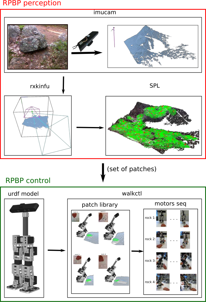
28 Rock Patch Tracking
For the first experiment we let the robot walk on a flat table using a predefined motion sequence. The table includes four rocks that do not come in contact with the robot during locomotion. When the robot is moving a map of patches is created. We split the whole environment into an grid and we let the map contain one seed point per cell. The purpose of this experiment is to understand whether the shaking and the vibrations affect the patch mapping and tracking process. For this we visually check particular patches (Figure 55) while the robot is moving, making sure that they are tracked correctly during the run. A more precise evaluation would be to quantitatively measure the camera drifts in a way similar to how the original moving volume Kinect Fusion system was validated [96, 132].

29 Foot Placement on Rock Patches
In the second experiment we test the ability of the robot to use the real-time patch mapping system integrated in a foot placement application. Our apparatus (Figure 56) includes a table with 4 solid rocks in fixed positions. The robot is always attached to a safety belay, but this does not affect its motion significantly, i.e. it does not hold it upright during the run. We developed a simple control system where the robot executes a set of predefined motions, we manually trained by creating a library of patches and a motion sequence for each.

Foot Placement Training
We let the lookdown robot pose, as appears in Figure 57, be the starting point for training on each rock. We place the robot in front of each of the four rocks in a defined position and we let the rxkinfu system provide us with a point cloud of the environment. For each rock we manually select a neighborhood where we would like the robot to place its foot and we fit a patch to it. The four patches we trained the robot to recognize, appear in Figure 57. For each one of them we train the robot to place its foot with a corresponding motion sequence as shown in Figure 58. For the training we used the the BRBrain library [158], which is more convenient for that purpose. In a similar way we could train the robot to place its feet on various other positions, but this goes beyond the intention of the experiment which focuses on perception, not control.


Foot Placement Test
The foot placement experiment proceeds as follows. We place the robot in the lookdown pose in front of each rock, roughly in the same position as it was trained in. We then let the perception system to create a patch map as it was described in Chapter 4, but using a different method for seed selection. Here we consider all the points within from the center of each trained patch3838 38 The trained patches are stored with poses defined relative to the robot. In this way we map patches close to what the robot is trained to step on. We then perform a patch matching. We compare every patch in the map with every trained patch. The similarity comparison between two patches proceeds as follows:
- 1.
Check whether the patches are of the same type (elliptic/hyperbolic/cylindric paraboloid or flat).
- 2.
Check whether the absolute difference between their boundary parameters are smaller than a threshold .
- 3.
Check whether the absolute difference between the curvatures are smaller than a threshold .
- 4.
Check whether the angle between their normal vectors ( axis) is smaller than a threshold .
- 5.
Check whether the distance between their position (translation vector) is smaller than a threshold .
For checking the angle between the normal vector we should consider any possible symmetry. For all patch types except planar and circular paraboloids, we need in addition to compare the angle between the axes using the same threshold , as well as the axes of the patches rotated around their axes. If any of the patch in the map matches with a trained one we execute the corresponding motion sequence.
We ran the experiment twenty times for each rock and the robot never failed to match the correct trained patch and successfully run the motion sequence for placing its foot every time. Success was defined as maintaining balance and ending with the foot on the rock. We also tried to place the robot in front of a few other rocks that it was not trained on and it stayed still, not having detected any patch match. An example is visualized in Figure 59 for the first rock, where the robot detects a match with the corresponding trained patch and executes the motion sequence. We also can see that the robot tracks very accurately a matched patch when it is moving. In the last step of the visualization the foot is placed in contact with the patch.

30 Related Work
The number of on-line perception systems for bipedal foot placement that are tested on real robots is very limited in the literature. We are not aware of work on a biped that includes perception for significantly curved surfaces like natural rocks. Though it is true that most current bipeds and humanoids have flat feet with limited ability to physically contact curved surfaces, this use case will become more important as more capable feet are developed [35]. Some work has been done for the case of flat surfaces. In a series of papers Okada et al. [100, 101, 102] developed a perception system for detecting flat surfaces and having various humanoids stepping on them. In their first paper a 16-DoF mini-humanoid that uses stereo vision data, detects planar segments that appear in various heights in front of the robot and performs a climbing step on them. In their second paper they apply the same plane detection system on the HOAP-1 humanoid robot for detecting floor regions, creating a local map of polygon patches that belong to the floor and step on them. In their third paper they apply their method on an HRP-2 robot for step climbing on horizontal flat surfaces. Gutmann et al. [37, 146, 38] have their QRIO robot detect and climb up and down on horizontal planar patches (mainly stairs) segmented using a point cloud. Chestnutt et al. [19] used 3D laser point cloud data for detecting horizontal obstacles of different heights in the environment and climb on and off, using their own prototype humanoid robot, while more recently in [99] HRP-2 was able to detect uneven flat surfaces with some slope and walk efficiently on them using dynamic ZMP-based walking motion. In a series of papers [83, 50, 82] and a thesis [49] the Humanoid Robots Lab in University of Freiburg has developed a system based on range sensing using a NAO robot for detecting flat obstacles and either step on or over them, using predefined motion primitives.
31 Summary and Future Work
In this chapter we presented experiments with our patch mapping and tracking system integrated on a real mini-biped for foot placement. Using a simple control system where the walking motion is a human trained combination of sequences, we first train the robot to place its foot on four different patches and then we let the robot create a patch map of its environment, find matches between the patches and the trained ones, and if any exist run the predefined sequence motion. A more advanced dynamic walking system requires balance control, possibly using the Zero Moment Point method [58] and appropriate path planning. For our experiments we assume that there are no collisions between the leg and any surface while executing the motion. The problem of generating collision-free motions is well studied (e.g. [50]) and we are not considering it for these experiments, though it would be required in practical applications.
Various other directions are possible for experimental validation of the patch mapping system on the robot, for instance a comparison between our perception algorithm with a proprioceptive blind robot that tries to complete the same task [159]. It is also necessary to consider different types of foot for curved surfaces contact. In our experiments we used flat feet, but a different design for a better contact, possibly using miltiple toes and/or compliance, may be preferable [35].
††margin: 7 Conclusions and Future Work
In real world applications articulated robots need to come in contact with unstructured environments either for locomotion or manipulation. In this thesis we introduced a novel perception system for modeling the contact areas between a robot and a rough surface and demonstrated its use in bipedal locomotion. Our system creates in real-time a map of bio-inspired salient bounded curved patches that fit to the environment in locations of potential footfall contact and tracks them when the robot is moving using an RGB-D depth camera and an IMU sensor.
We envision our method to be part of a bigger system where not only foot placement, but also other types of contact (for instance dexterous manipulation) is driven using similar patches. In this thesis we developed experiments which prove that the robot can find contact patches for footfall placement, but as explained in Chapter 6 high level path planning along with a more advanced control system is required for dynamic walking using these patches. Furthermore, it is also interesting to understand how the patch uncertainty can play a role not only for data fusion while the robot is moving, but also for foot placement decisions. For instance a highly uncertain patch may not be considered for foot placement, or the motor compliance may be adapted with respect to the level of patch uncertainty. Last but not least, a mapping and tracking method (e.g. [148, 66]) that does not use a GPU device (which is not always available in all autonomous robots) instead of the Kinect Fusion system may need to be used.
Part III Appendix
††margin: 8 Environment Representation
Appendix 8.A Jacobians
We calculate the Jacobian of the exponential map (13) as a row tensor3939 39 (72) remains finite as . Small angle approximations for and were given in Section 7.2; their derivatives can be approximated as and .:
| (72) | |||
Viewing (22) as a vector function,
its Jacobian is where block from right to left is, with from (21), from (22), from Appendix 8.B,
| (74) |
| (75) |
Appendix 8.B The Logarithmic Map
Due to numerical issues with other equations we found in the literature, we developed the following numerically stable algorithm to calculate the log map
and its column tensor Jacobian .
Appendix 8.C Patch Fit Uncertainty Propagation
During the fitting process the covariance matrix of the patch parameters is calculated by first order error propagation [92] using the Gaussian uncertainty model as follows. In each step the input covariance matrix will either come from the WLM fitting or from the previous step.
- Stage I:
Fit an Unbounded Surface
- Step 1:
Plane fitting
Input: , , (from the WLM fitting)
Output:Let
The propagated covariance is:
(76) where
(77) and
(78) - Step 2:
Surface Fitting
If Equation (45) is enabled for the side-wall effect, then the input is replaced by , where with .If (s = sphere)
Input: , k, , (from the WLM fitting)
Output:(79) where
(80) If (s = circ cyl)
Input: (log map), , , ,
Output:(81) where
(82) and
(83) - Step 3:
Curvature Discrimination (if )
If ()
Input: ,
Output:(84) where
(85) Else if ()
If
Input: ,
Output:(86) where
(87) Else swap axes
Input: , (log map),
Output:(88) where
(89) Else if ()
Input: , ,
Output:(90) where
(91) Else ()
No change in , , and
- Step 1:
- Stage II:
Fit the Boundary
- Step 5:
Initialize Bounding Parameters
Input: ,
Output:Let
(92) where
(93) where
(94)
- Step 6:
Cylindrical Paraboloid and Circular Cylinder Boundary Fitting
Input: , ,
Output:(95) where
(96) - Step 7:
Circular Paraboloid and Sphere Boundary Fitting
Input: ,
Output:(97) where
(98) If , then
Else if , then
Else , then
- Step 8:
Elliptic and Hyperbolic Boundary Fitting
Input: ,
Output:(99) where
(100)
- Step 9:
Plane Boundary Fitting (if )
Input: , , , ,
Output:Let
The covariance matrix is:
(101) where
(102) - 1.
If
Input: ,
Output:(103) where
(104) if , then and
if , then and
if , then and - 2.
If
Input: ,
Output:
Let .(105) where
(106) If
If
- 1.
- Step 5:
Appendix 8.D Taubin’s Residual Approximations
The distance of a point from a paraboloid whose implicit (local) form is , using the first order Taubin’s [152] approximation is:
| (107) | |||
Using the second order Taubin approximation the distance is computed in three steps:
- 1.
Taylor series coefficient computation
- 2.
Fh(p) computation for h=1,2
- 3.
Solve for the min positive root of:
(108) where is the approximate min Euclidean distance.
References
- [1] Sung Joon Ahn, Wolfgang Rauh, Hyung Suck Cho, and Hans-Jürgen Warnecke. Orthogonal Distance Fitting of Implicit Curves and Surfaces. IEEE Trans. Pattern Anal. Mach. Intell., 24(5):620–638, 2002.
- [2] A Bab-Hadiashar and N. Gheissari. Range Image Segmentation using Surface Selection Criterion. Image Processing, IEEE Transactions on, 15(7):2006–2018, July 2006. ISSN 1057-7149. 10.1109/TIP.2006.877064.
- [3] Kwang-Ho Bae, David Belton, and Derek D. Lichti. A Closed-Form Expression of the Positional Uncertainty for 3D Point Clouds. IEEE Transactions on Pattern Analysis and Machine Intelligence, 31(4):577–590, 2009. ISSN 0162-8828. http://doi.ieeecomputersociety.org/10.1109/TPAMI.2008.116.
- [4] J. Bares, M. Hebert, T. Kanade, E. Krotkov, T. Mitchell, R. Simmons, and W. Whittaker. Ambler—An Autonomous Rover for Planetary Exploration. IEEE Computer, 22:18–26, 1989.
- [5] John Bares and David Wettergreen. Dante II: Technical Description, Results, and Lessons Learned. Int. J. Robotic Research, 18(7):621–649, 1999.
- [6] Sven Behnke. Humanoid Robots – From Fiction to Reality? KI–Zeitschrift, 04/08:5–9, December 2008.
- [7] D Belter and P Skrzypczynski. Precise Self-Localization of a Walking Robot on Rough Terrain Using PTAM. In Adaptive Mobile Robotics, pages 89–96. World Scientific, 2012.
- [8] Dominik Belter, Przemysław Łabȩcki, and Piotr Skrzypczynski. Map-based Adaptive Foothold Planning for Unstructured Terrain Walking. In 2010 IEEE International Conference on Robotics and Automation (ICRA), pages 5256–5261, 2010.
- [9] Jon Louis Bentley. Multidimensional Binary Search Trees Used for Associative Searching. Communications of the ACM, 18(9):509–517, 1975. ISSN 0001-0782.
- [10] C. Berger and S. Lacroix. Using Planar Facets for Stereovision SLAM. In Intelligent Robots and Systems, 2008. IROS 2008. IEEE/RSJ International Conference on, pages 1606–1611, Sept 2008. 10.1109/IROS.2008.4650986.
- [11] Michael M. Blane, Zhibi Lei, Hakan Çivi, and David B. Cooper. The 3L Algorithm for Fitting Implicit Polynomial Curves and Surfaces to Data. IEEE Trans. Pattern Anal. Mach. Intell., 22(3):298–313, Mar 2000. ISSN 0162-8828. 10.1109/34.841760.
- [12] Morten Rufus Blas, Mogens Blanke, Radu Bogan Rusu, and Michael Beetz. Fault-tolerant 3D Mapping with Application to an Orchard Robot, pages 893–898. 2009. ISBN 978-3-902661-46-3. 10.3182/20090630-4-ES-2003.00147.
- [13] Dr. Gary Rost Bradski and Adrian Kaehler. Learning Opencv. O’Reilly Media, Inc., first edition, 2008. ISBN 9780596516130.
- [14] R. W. Brockett. Robotic Manipulators and the Product of Exponentials Formula, 1983.
- [15] Ted J. Broida and R. Chellappa. Estimation of Object Motion Parameters from Noisy Images. Pattern Analysis and Machine Intelligence, IEEE Transactions on, PAMI-8(1):90–99, Jan 1986. ISSN 0162-8828. 10.1109/TPAMI.1986.4767755.
- [16] Rodney Brooks. Robotics. March 2009.
- [17] Stanislas Brossette, Joris Vaillant, Francois Keith, Adrien Escande, and Abderrahmane Kheddar. Point-Cloud Multi-Contact Planning for Humanoids: Preliminary Results. In In the proceedings of Cybarnetics and Intelligent Systems Robotics, Automation and Mechatronics (CISRAM), volume 1, page 6, 2013.
- [18] Joel Chestnutt, Manfred Lau, German Cheung, James Kuffner, Jessica Hodgins, and Takeo Kanade. Footstep Planning for the Honda ASIMO Humanoid. In Proceedings of the 2005 IEEE International Conference on Robotics and Automation (ICRA), pages 629–634, 2005.
- [19] Joel Chestnutt, Yutaka Takaoka, Keisuke Suga, Koichi Nishiwaki, James Kuffner, and Satoshi Kagami. Biped Navigation in Rough Environments Using On-board Sensing. In Proceedings of the 2009 IEEE/RSJ International Conference on Intelligent Robots and Systems, IROS’09, pages 3543–3548, Piscataway, NJ, USA, 2009. IEEE Press. ISBN 978-1-4244-3803-7.
- [20] Chee-Meng Chew, J. Pratt, and G. Pratt. Blind Walking of a Planar Bipedal Robot on Sloped Terrain. In Proceedings of IEEE ICRA, volume 1, pages 381–386, 1999.
- [21] Brian Curless and Marc Levoy. A Volumetric Method for Building Complex Models from Range Images. In Proceedings of the 23rd Annual Conference on Computer Graphics and Interactive Techniques, SIGGRAPH ’96, pages 303–312, New York, NY, USA, 1996. ACM. ISBN 0-89791-746-4. 10.1145/237170.237269. URL http://doi.acm.org/10.1145/237170.237269.
- [22] Min Dai, Timothy S. Newman, and Chunguang Cao. Least-Squares-Based Fitting of Paraboloids. Pattern Recognition, 40:504–515, 2007.
- [23] C. Dorai, J. Weng, and A.K. Jain. Optimal Registration of Object Views Using Range Data. Pattern Analysis and Machine Intelligence, IEEE Transactions on, 19(10):1131–1138, Oct 1997. ISSN 0162-8828. 10.1109/34.625115.
- [24] Finale Doshi, Emma Brunskill, Alexander C. Shkolnik, Thomas Kollar, Khashayar Rohanimanesh, Russ Tedrake, and Nicholas Roy. Collision Detection in Legged Locomotion using Supervised Learning. In IEEE/RSJ International Conference on Intelligent Robots and Systems (IROS), pages 317–322, 2007.
- [25] Ivan Dryanovski, Roberto G. Valenti, and Jizhong Xiao. Fast Visual Odometry and Mapping from RGB-D Data. In 2013 IEEE International Conference on Robotics and Automation (ICRA), pages 2305–2310, May 2013. 10.1109/ICRA.2013.6630889.
- [26] H. Durrant-Whyte and Tim Bailey. Simultaneous Localization and Mapping: Part I,II. Robotics Automation Magazine, IEEE, 13(2):99–110, June 2006. ISSN 1070-9932. 10.1109/MRA.2006.1638022.
- [27] David Eberly. Distance from Point to a General Quadratic Curve or a General Quadric Surface. Technical report, 1999.
- [28] D.W. Eggert, A. Lorusso, and R.B. Fisher. Estimating 3-D Rigid Body Transformations: a Comparison of Four Major Algorithms. Machine Vision and Applications, 9(5–6):272–290, 1997. ISSN 0932-8092. 10.1007/s001380050048.
- [29] F. Endres, J. Hess, N. Engelhard, J. Sturm, D. Cremers, and W. Burgard. An Evaluation of the RGB-D SLAM System. In Proc. of the IEEE Int. Conf. on Robotics and Automation (ICRA), St. Paul, MA, USA, May 2012.
- [30] H. R. Everett. Sensors for Mobile Robots: Theory and Application. A. K. Peters, Ltd., Natick, MA, USA, 1995. ISBN 1-56881-048-2.
- [31] O. Faugeras, N. Ayache, and B. Faverjon. Building Visual Maps by Combining Noisy Stereo Measurements. In Robotics and Automation. Proceedings. 1986 IEEE International Conference on, volume 3, pages 1433–1438, Apr 1986. 10.1109/ROBOT.1986.1087419.
- [32] O. D. Faugeras and M. Hebert. Segmentation of Range Data into Planar and Quadratic Patches. In Proceedings of IEEE Conference on Computer Vision and Pattern Recognition, pages 8–13, Arlington, VA, June 1983.
- [33] P. Filitchkin and K. Byl. Feature-Based Terrain Classification for LittleDog. In 2012 IEEE/RSJ International Conference on Intelligent Robots and Systems (IROS), pages 1387–1392, 2012. 10.1109/IROS.2012.6386042.
- [34] Donald Bernard Gennery. Modelling the Environment of an Exploring Vehicle by Means of Stereo Vision. PhD thesis, Stanford, CA, USA, 1980. AAI8024660.
- [35] Sergio Castro Gomez. Sensing with a 3-Toe Foot for a Mini-Biped Robot. Master’s thesis, ECE, Northeastern University, 2014.
- [36] F. Sebastian Grassia. Practical Parameterization of Rotations using the Exponential Map. J. Graphics Tools, 3(3):29–48, 1998. ISSN 1086-7651.
- [37] Jens-Steffen Gutmann, Masaki Fukuchi, and Masahiro Fujita. Stair Climbing for Humanoid Robots Using Stereo Vision. In Proceedings of IEEE/RSJ International Conference on Intelligent Robots and Systems (IROS), pages 1407–1413, 2004.
- [38] Jens-Steffen Gutmann, Masaki Fukuchi, and Masahiro Fujita. 3D Perception and Environment Map Generation for Humanoid Robot Navigation. International Journal of Robotics Research, 27(10):1117–1134, 2008. ISSN 0278-3649.
- [39] Inyong Ha, Yusuke Tamura, H. Asama, Jeakweon Han, and D.W. Hong. Development of Open Humanoid Platform DARwIn-OP. In SICE Annual Conference (SICE), 2011 Proceedings of, pages 2178–2181, Sept 2011.
- [40] John Hallam. Resolving Observer Motion by Object Tracking. In Proceedings of the Eighth International Joint Conference on Artificial Intelligence - Volume 2, IJCAI’83, pages 792–798, San Francisco, CA, USA, 1983. Morgan Kaufmann Publishers Inc.
- [41] Eyal Hameiri and Ilan Shimshoni. Estimating the Principal Curvatures and the Darboux Frame from Real 3D Range Data. In 3DPVT, pages 258–267, 2002.
- [42] P. Hebert, D. Laurendeau, and D. Poussart. Scene reconstruction and description: geometric primitive extraction from multiple viewed scattered data. In Computer Vision and Pattern Recognition, 1993. Proceedings CVPR ’93., 1993 IEEE Computer Society Conference on, pages 286–292, Jun 1993. 10.1109/CVPR.1993.340967.
- [43] Amir Helzer, Meir Barzohar, and David Malah. Stable Fitting of 2D Curves and 3D Surfaces by Implicit Polynomials. IEEE Trans. Pattern Anal. Mach. Intell., 26(10):1283–1294, Oct 2004. ISSN 0162-8828. 10.1109/TPAMI.2004.91. URL http://dx.doi.org/10.1109/TPAMI.2004.91.
- [44] Francisco Heredia and Raphael Favier. Kinfu Large Scale in PCL, 2012. URL http://www.pointclouds.org/blog/srcs.
- [45] M.A. Hollands and D.E. Marple-Horvat. Visually Guided Stepping under Conditions of Step Cycle-Related Denial of Visual Information. Experimental Brain Research, pages 343–356, 1996.
- [46] Stefan Holzer, Radu Bogdan Rusu, M. Dixon, Suat Gedikli, and Nassir Navab. Adaptive Neighborhood Selection for Real-Time Surface Normal Estimation from Organized Point Cloud Data Using Integral Images. In IEEE/RSJ International Conference on Intelligent Robots and Systems (IROS), pages 2684–2689, 2012.
- [47] Adam Hoover, Gillian Jean-Baptiste, Xiaoyi Jiang, Patrick J. Flynn, Horst Bunke, Dmitry Goldgof, Kevin Bowyer, David Eggert, Andrew Fitzgibbon, and Robert Fisher. An Experimental Comparison of Range Image Segmentation Algorithms. IEEE Transactions on Pattern Analysis and Machine Intelligence, 18(7):673–689, 1996.
- [48] Takehiro Horiuchi, Masatomo Kanehara, Satoshi Kagami, and Yoshihiro Ehara. A Probabilistic Walk Path Model Focused On Foot Landing Points And Human Step Measurement System. In SMC, pages 109–114, 2006. ISBN 1-4244-0099-6.
- [49] Armin Hornung. Humanoid Robot Navigation in Complex Indoor Environments. PhD thesis, University of Freiburg, 2014.
- [50] Armin Hornung, Daniel Maier, and Maren Bennewitz. Search-Based Footstep Planning. In Proceedings of the ICRA Workshop on Progress and Open Problems in Motion Planning and Navigation for Humanoids, 2013.
- [51] Andrew Howard. Real-time Stereo Visual Odometry for Autonomous Ground Vehicles. In IEEE/RSJ Int. Conf. on Intelligent Robots and Systems, 2008.
- [52] T. Huang, G. Yang, and G. Tang. A Fast Two-Dimensional Median Filtering Algorithm. Acoustics, Speech and Signal Processing, IEEE Transactions on, 27(1):13–18, Feb 1979. ISSN 0096-3518.
- [53] Yani Ioannou, Babak Taati, Robin Harrap, and Michael A. Greenspan. Difference of Normals as a Multi-Scale Operator in Unorganized Point Clouds. CoRR, abs/1209.1759, 2012.
- [54] Shahram Izadi, David Kim, Otmar Hilliges, David Molyneaux, Richard Newcombe, Pushmeet Kohli, Jamie Shotton, Steve Hodges, Dustin Freeman, Andrew Davison, and Andrew Fitzgibbon. KinectFusion: Real-time 3D Reconstruction and Interaction Using a Moving Depth Camera. In Proceedings of the 24th Annual ACM Symposium on User Interface Software and Technology, UIST ’11, pages 559–568, New York, NY, USA, 2011. ACM. ISBN 978-1-4503-0716-1. 10.1145/2047196.2047270. URL http://doi.acm.org/10.1145/2047196.2047270.
- [55] S. Jajita and T. Sugihara. Humanoid Robots in the Future. Advanced Robotics, 23:1527–1531, 2009.
- [56] Xiaoyi Jiang and Horst Bunke. Fast Segmentation of Range Images into Planar Regions by Scan Line Grouping. Machine Vision and Application, 7(2):115–122, 1994.
- [57] Andrew Edie Johnson and Sing Bing Kang. Registration and Integration of Textured 3-D Data. In Proceedings of the International Conference on Recent Advances in 3-D Digital Imaging and Modeling, NRC ’97, pages 234–241, Washington, DC, USA, 1997. IEEE Computer Society. ISBN 0-8186-7943-3.
- [58] S. Kajita, F. Kanehiro, K. Kaneko, K. Fujiwara, K. Harada, K. Yokoi, and H. Hirukawa. Biped Walking Pattern Generation by using Preview Control of Zero-Moment Point. In Robotics and Automation, 2003. Proceedings. ICRA ’03. IEEE International Conference on, volume 2, pages 1620–1626, Sept 2003. 10.1109/ROBOT.2003.1241826.
- [59] M. Kalakrishnan, J. Buchli, P. Pastor, and S. Schaal. In IEEE/RSJ International Conference on Intelligent Robots and Systems (IROS), pages 167–172, 2009.
- [60] M. Kalakrishnan, J. Buchli, P. Pastor, M. Mistry, and S. Schaal. Learning, Planning, and Control for Quadruped Locomotion over Challenging Terrain. International Journal of Robotics Research, (2):236–258, 2010.
- [61] Kenichi Kanatani. Statistical Optimization for Geometric Computation: Theory and Practice. Dover Publications, Incorporated, 2005. ISBN 0486443086.
- [62] Dimitrios Kanoulas and Marsette Vona. Surface Patch Library (SPL), 2011. http://ccis.neu.edu/research/gpc/spl.
- [63] Dimitrios Kanoulas and Marsette Vona. Sparse Surface Modeling with Curved Patches. In Proceedings of the IEEE International Conference on Robotics and Automation (ICRA), 2013.
- [64] Dimitrios Kanoulas and Marsette Vona. Bio-Inspired Rough Terrain Contact Patch Perception. In Proceedings of the IEEE International Conference on Robotics and Automation (ICRA), 2014.
- [65] Dov Katz, Jacqueline Kenney, and Oliver Brock. How Can Robots Succeed in Unstructured Environments. In Workshop on Robot Manipulation: Intelligence in Human Environments at Robotics, Zurich, Switzerland, June 2008. Science and Systems.
- [66] C. Kerl, J. Sturm, and D. Cremers. Dense Visual SLAM for RGB-D Cameras. In Proc. of the Int. Conf. on Intelligent Robot Systems (IROS), 2013.
- [67] Oussama Khatib and Shu-Yun Chung. SupraPeds: Humanoid Contact-Supported Locomotion for 3D Unstructured Environments. In Proceedings of the IEEE International Conference on Robotics and Automation (ICRA), 2014.
- [68] Kourosh Khoshelham. Accuracy Analysis of Kinect Depth Data. ISPRS Workshop Laser Scanning, 38(5):W12, 2011.
- [69] Kourosh Khoshelham and Sander Oude Elberink. Accuracy and Resolution of Kinect Depth Data for Indoor Mapping Applications. In Sensors, volume 12, pages 1437–1454, 2012.
- [70] Georg Klein and David Murray. Parallel Tracking and Mapping for Small AR Workspaces. In Proc. Sixth IEEE and ACM International Symposium on Mixed and Augmented Reality (ISMAR’07), Nara, Japan, November 2007.
- [71] Georg Klein and David Murray. Parallel Tracking and Mapping on a Camera Phone. In Proc. Eigth IEEE and ACM International Symposium on Mixed and Augmented Reality (ISMAR’09), Orlando, October 2009.
- [72] J. Zico Kolter, Youngjun Kim, and Andrew Y. Ng. Stereo Vision and Terrain Modeling for Quadruped Robots. In Proceedings of the 2009 IEEE International Conference on Robotics and Automation (ICRA), pages 3894–3901, 2009a.
- [73] J. Zico Kolter, Youngjun Kim, and Andrew Y. Ng. Stereo Vision and Terrain Modeling for Quadruped Robots. In IEEE IEEE International Conference on Robotics and Automation (ICRA), pages 1557–1564, 2009b. 10.1109/ROBOT.2009.5152795.
- [74] Kurt Konolige and Patrick Mihelich. Technical description of kinect calibration, 2010. http://www.ros.org/wiki/kinect_calibration/technical.
- [75] Eric Krotkov and Reid G. Simmons. Perception, Planning, and Control for Autmonomous Walking with the Ambler Planetary Rover. Int. J. Robotics Research, 15(2):155–180, 1996.
- [76] J. Lam and M. Greenspan. On the Repeatability of 3D Point Cloud Segmentation Based on Interest Points. In Computer and Robot Vision (CRV), 2012 Ninth Conference on, pages 9–16, 2012. 10.1109/CRV.2012.9.
- [77] Tobias Lang, Christian Plagemann, and Wolfram Burgard. Adaptive Non-Stationary Kernel Regression for Terrain Modelling. In Robotics: Science and Systems, 2007.
- [78] Chang Ha Lee, Amitabh Varshney, and David W. Jacobs. Mesh Saliency. In ACM SIGGRAPH, pages 659–666, New York, NY, USA, 2005. ACM.
- [79] M. Anthony Lewis, Hyo-Kyung Lee, and Aftab Patla. Foot Placement Selection using Non-geometric Visual Properties. The International Journal of Robotics Research, 24:553–561, July 2005.
- [80] Yu-Shen Liu, Min Liu, Daisuke Kihara, and Karthik Ramani. Salient Critical Points for Meshes. In Proceedings of the 2007 ACM Symposium on Solid and Physical Modeling (SPM), pages 277–282, New York, NY, USA, 2007.
- [81] William E. Lorensen and Harvey E. Cline. Marching cubes: A high resolution 3d surface construction algorithm. In Proceedings of the 14th Annual Conference on Computer Graphics and Interactive Techniques, SIGGRAPH ’87, pages 163–169, New York, NY, USA, 1987. ACM. ISBN 0-89791-227-6. 10.1145/37401.37422. URL http://doi.acm.org/10.1145/37401.37422.
- [82] D. Maier, C. Lutz, and M. Bennewitz. Integrated Perception, Mapping, and Footstep Planning for Humanoid Navigation Among 3D Obstacles. In Proceedings of IEEE/RSJ International Conference on Intelligent Robots and Systems IROS, 2013.
- [83] Daniel Maier, Armin Hornung, and Maren Bennewitz. Real-Time Navigation in 3D Environments Based on Depth Camera Data. In Proceedings of the IEEE-RAS International Conference on Humanoid Robots (HUMANOIDS), Osaka, Japan, November 2012.
- [84] Mark W. Maimone, P. Chris Leger, and Jeffrey J. Biesiadecki. Overview of the Mars Exploration Rovers Autonomous Mobility and Vision Capabilities. In IEEE International Conference on Robotics and Automation (ICRA, 2007.
- [85] Daniel S. Marigold. Role Of Peripheral Visual Cues In Online Visual Guidance Of Locomotion. Exercise Sport Science Reviews, pages 145–151, 2008.
- [86] Daniel S. Marigold and Aftab E. Patla. Gaze Fixation Patterns for Negotiating Complex Ground Terrain. Neuroscience, pages 302–313, 2007.
- [87] Daniel S. Marigold and Aftab E. Patla. Visual Information from the Lower Visual Field is Important for Walking Across Multi-Surface Terrain. Exp Brain Res, 188:23–31, 2008.
- [88] Matthew T. Mason. Creation Myths: The Beginnings of Robotics Research. IEEE Robotics & Automation Magazine, 19(2):72–77, 2012.
- [89] Matthew T. Mason and J. Kenneth Salisbury, Jr. Robot Hands and the Mechanics of Manipulation. MIT Press, 1985. ISBN 0-262-13205-2.
- [90] Larry Matthies and Steven A. Shafer. Error Modeling in Stereo Navigation. pages 135–144, 1990. 10.1007/978-1-4613-8997-2_12.
- [91] Stefan May, David Droeschel, Dirk Holz, Christoph Wiesen, and Stefan Fuchs. 3D Pose Estimation and Mapping with Time-of-Flight Cameras. In IEEE/RSJ International Conference on Intelligent Robots and Systems (IROS), Workshop on 3D Mapping, Nice, France, October 2008.
- [92] Stuart L. Meyer. Data Analysis for Scientists and Engineers. Peer Management Consultants, Ltd., 1992.
- [93] N. D. Molton, A. J. Davison, and I. D. Reid. Locally Planar Patch Features for Real-Time Structure from Motion. In Proc. British Machine Vision Conference. BMVC, Sep 2004.
- [94] Michael E. Mortenson. Geometric Modeling. Industrial Press, 2006.
- [95] Don Murray and James J. Little. Patchlets: Representing Stereo Vision Data with Surface Elements. In Proceedings of the Seventh IEEE Workshops on Application of Computer Vision (WACV/MOTION’05) - Volume 1 - Volume 01, WACV-MOTION ’05, pages 192–199, Washington, DC, USA, 2005. IEEE Computer Society. ISBN 0-7695-2271-8-1. 10.1109/ACVMOT.2005.90. URL http://dx.doi.org/10.1109/ACVMOT.2005.90.
- [96] Richard A. Newcombe, Shahram Izadi, Otmar Hilliges, David Molyneaux, David Kim, Andrew J. Davison, Pushmeet Kohli, Jamie Shotton, Steve Hodges, and Andrew Fitzgibbon. KinectFusion: Real-Time Dense Surface Mapping and Tracking. In IEEE International Symposium on Mixed and Augmented Reality (ISMAR). IEEE, October 2011a.
- [97] Richard A. Newcombe, Steven J. Lovegrove, and Andrew J. Davison. DTAM: Dense Tracking and Mapping in Real-time. In Proceedings of the 2011 International Conference on Computer Vision, ICCV ’11, pages 2320–2327, Washington, DC, USA, 2011b. IEEE Computer Society. ISBN 978-1-4577-1101-5. 10.1109/ICCV.2011.6126513. URL http://dx.doi.org/10.1109/ICCV.2011.6126513.
- [98] Xinlai Ni, Michael Garland, and John C. Hart. Fair Morse Functions for Extracting the Topological Structure of a Surface Mesh. In ACM SIGGRAPH 2004 Papers, SIGGRAPH ’04, pages 613–622, New York, NY, USA, 2004. ACM. 10.1145/1186562.1015769. URL http://doi.acm.org/10.1145/1186562.1015769.
- [99] Koichi Nishiwaki, Joel E. Chestnutt, and Satoshi Kagami. Autonomous Navigation of a Humanoid Robot over Unknown Rough Terrain using a Laser Range Sensor. International Journal of Robotic Research, 31(11):1251–1262, 2012.
- [100] K. Okada, S. Kagami, M. Inaba, and H. Inoue. Plane Segment Finder: Algorithm, Implementation and Applications. In Robotics and Automation, 2001. Proceedings 2001 ICRA. IEEE International Conference on, volume 2, pages 2120–2125, 2001. 10.1109/ROBOT.2001.932920.
- [101] K. Okada, M. Inaba, and H. Inoue. Walking Navigation System of Humanoid Robot Using Stereo Vision Based Floor Recognition and Path Planning with Multi-Layered Body Image. In Proceedings. 2003 IEEE/RSJ International Conference on Intelligent Robots and Systems, 2003. (IROS 2003), volume 3, pages 2155–2160, 2003. 10.1109/IROS.2003.1249190.
- [102] K. Okada, T. Ogura, A Haneda, and M. Inaba. Autonomous 3D Walking System for a Humanoid Robot Based on Visual Step Recognition and 3D Foot Step Planner. In Robotics and Automation, 2005. ICRA 2005. Proceedings of the 2005 IEEE International Conference on, pages 623–628, April 2005. 10.1109/ROBOT.2005.1570187.
- [103] IEEE RAS Technical Committee on Mobile Manipulation. Mission statement, 2013. URL http://www.mobilemanipulation.org.
- [104] Paul Ozog and Ryan M. Eustice. Real-time SLAM with Piecewise-Planar Surface Models and Sparse 3D Point Clouds. In Proceedings of the IEEE/RSJ International Conference on Intelligent Robots and Systems, pages 1042–1049, Tokyo, Japan, November 2013. http://dx.doi.org/10.1109/IROS.2013.6696479.
- [105] Jia Pan, Sachin Chitta, and Dinesh Manocha. Probabilistic Collision Detection between Noisy Point Clouds using Robust Classification. In International Symposium on Robotics Research, Flagstaff, Arizona, August 2011.
- [106] Sylvain Paris and Frédo Durand. A Fast Approximation of the Bilateral Filter using a Signal Processing Approach. In In Proceedings of the European Conference on Computer Vision, pages 568–580, 2006.
- [107] Frank C. Park. Computational aspects of the product-of-exponentials formula for robot kinematics. IEEE Transactions on Automatic Control, 39(3):643–647, 1994.
- [108] Steven Parker, Peter Shirley, Yarden Livnat, Charles Hansen, and Peter-Pike Sloan. Interactive ray tracing for isosurface rendering. In Proceedings of the Conference on Visualization ’98, Proceedings of Visualization (VIS) ’98, pages 233–238, Los Alamitos, CA, USA, 1998. IEEE Computer Society Press. ISBN 1-58113-106-2. URL http://dl.acm.org/citation.cfm?id=288216.288266.
- [109] B. Parvin and G. Medioni. Segmentation of Range Images into Planar Surfaces by Split and Merge. In Proceedings of Computer Society Conference on on Computer Vision and Pattern Recognition, pages 415–417, 1986.
- [110] K. Pathak, N. Vaskevicius, and A. Birk. Revisiting Uncertainty Analysis for Optimum Planes Extracted from 3D Range Sensor Point-Clouds. In IEEE International Conference on Robotics and Automation (ICRA), pages 1631–1636, 2009. 10.1109/ROBOT.2009.5152502.
- [111] Kaustubh Pathak, Andreas Birk, Narunas Vaskevicius, Max Pfingsthorn, and Soren Schwertfeger. Online 3D SLAM by Registration of Large Planar Surface Segments and Closed form Pose-Graph Relaxation. Journal of Field Robotics: Special Issue on 3D Mapping, 27(1):52–84, 2010.
- [112] A.E. Patla. Understanding the Roles of Vision in the Control of Human Locomotion. Gait and Posture, pages 54–69, 1997.
- [113] A.E. Patla and J.N. Vickers. Where and When do we Look as we Approach and Step over an Obstacle in the Travel Path? Neuroreport, pages 3661–3665, 1997.
- [114] M. Pauly, N. J. Mitra, and L. Guibas. Uncertainty and Variability in Point Cloud Surface Data. In Symposium on Point-Based Graphics, pages 77–84, 2004.
- [115] Mark Pauly, Markus Gross, and Leif P. Kobbelt. Efficient Simplification of Point-Sampled Surfaces. In Proceedings of the Conference on Visualization (VIS), pages 163–170, Washington, DC, USA, 2002. IEEE Computer Society. ISBN 0-7803-7498-3.
- [116] S. Perreault and P. Hebert. Median Filtering in Constant Time. Image Processing, IEEE Transactions on, 16(9):2389–2394, Sept 2007. ISSN 1057-7149. 10.1109/TIP.2007.902329.
- [117] N. Perrin, O. Stasse, L. Baudouin, F. Lamiraux, and E. Yoshida. Fast Humanoid Robot Collision-Free Footstep Planning Using Swept Volume Approximations. IEEE Transactions on Robotics, 28:427–439, 2012.
- [118] Sylvain Petitjean. A Survey of Methods for Recovering Quadrics in Triangle Meshes. ACM Computing Surveys, 34:211–262, 2002.
- [119] Tuan Q. Pham. Non-Maximum Suppression using Fewer than two Comparisons per Pixel. In ACIVS (1), pages 438–451, 2010.
- [120] Christian Plagemann, Sebastian Mischke, Sam Prentice, Kristian Kersting, Nicholas Roy, and Wolfram Burgard. Learning Predictive Terrain Models for Legged Robot Locomotion. In IEEE/RSJ International Conference on Intelligent Robots and Systems (IROS), pages 3545–3552, 2008.
- [121] Christian Plagemann, Sebastian Mischke, Sam Prentice, Kristian Kersting, Nicholas Roy, and Wolfram Burgard. A Bayesian Regression Approach to Terrain Mapping and an Application to Legged Robot Locomotion. Journal of Field Robotics, 26:789–811, 2009.
- [122] Jean Ponce, David J. Kriegman, Sylvain Petitjean, Steven Sullivan, Gabriel Taubin, and B. Vijayakumar. Representations and Algorithms for 3D Curved Object Recognition. In P. Flynn and A. Jain, editors, Three-Dimensional Object Recognition Systems, pages 327–352. Elsevier Press, 1993.
- [123] Mark W. Powell, Kevin W. Bowyer, Xiaoyi Jiang, and Horst Bunke. Comparing Curved-Surface Range Image Segmenters. In ICCV ’98: Proceedings of the Sixth International Conference on Computer Vision, Washington, DC, USA, 1998. IEEE Computer Society. ISBN 81-7319-221-9.
- [124] William H. Press, Saul A. Teukolsky, William T. Vetterling, and Brian P. Flannery. Numerical Recipes in C (2nd ed.): the Art of Scientific Computing. Cambridge University Press, New York, NY, USA, 1992. ISBN 0-521-43108-5.
- [125] Marc Raibert, Kevin Blankespoor, Gabriel Nelson, Rob Playter, and the BigDog Team. BigDog, The Rough-Terrain Quadruped Robot. Proceedings of the 17th World Congress of the International Federation of Automatic Control, pages 10822–10825, July 2008.
- [126] O. E. Ramos, M. García, N. Mansard, O. Stasse, J-B. Hayet, and P. Souères. Towards Reactive Vision-Guided Walking on Rough Terrain: An Inverse-Dynamics Based Approach. In Workshop on Visual Navigation for Humanoid Robots (IEEE ICRA), Karlsruhe, Germany, May 2013.
- [127] M. I. Ribeiro. Gaussian Probability Density Functions: Properties and Error Characterization. Technical Report 1049-001, Instituto Superior Tcnico, 2004.
- [128] Shirley Rietdyk and Chris K. Rhea. Control of Adaptive Locomotion: Effect of Visual Obstruction and Visual Cues in the Environment. Experimental Brain Research, pages 272–278, 2006.
- [129] Lourena Rocha, Luiz Velho, and Paulo Cezar P. Carvalho. Image moments-based structuring and tracking of objects. In Brazilian Symposium on Computer Graphics and Image Processing, 2002.
- [130] A. Roennau, T. Kerscher, and R. Dillmann. Design and Kinematics of a Biologically-Inspired Leg for a Six-Legged Walking Machine. In 2010 3rd IEEE RAS and EMBS International Conference on Biomedical Robotics and Biomechatronics (BioRob), pages 626–631, 2010. 10.1109/BIOROB.2010.5626328.
- [131] Robot Operating System (ROS). Unified Robot Description Format (URDF), 2014. http://wiki.ros.org/urdf.
- [132] Henry Roth and Marsette Vona. Moving Volume KinectFusion. In British Machine Vision Conference, 2012.
- [133] Radu Bogdan Rusu and Steve Cousins. 3D is here: Point Cloud Library (PCL). In Proceedings of the IEEE International Conference on Robotics and Automation (ICRA), Shanghai, China, 2011.
- [134] Radu Bogdan Rusu, Michael Beetz, Zoltan Csaba Marton, Nico Blodow, and Mihai Dolha. Towards 3D Point Cloud Based Object Maps for Household Environments. Robotics and Autonomous Systems Journal (Special Issue on Semantic Knowledge), 2008.
- [135] Radu Bogdan Rusu, Andreas Holzbach, Rosen Diankov, Gary Bradski, and Michael Beetz. Perception for Mobile Manipulation and Grasping using Active Stereo. In IEEE-RAS Humanoids, 2009.
- [136] D. Scaramuzza and F. Fraundorfer. Visual Odometry [Tutorial]. Robotics Automation Magazine, IEEE, 18(4):80–92, Dec 2011. ISSN 1070-9932. 10.1109/MRA.2011.943233.
- [137] Daniel Scharstein and Richard Szeliski. A Taxonomy and Evaluation of Dense Two-Frame Stereo Correspondence Algorithms. International Journal of Computer Vision, 47(1-3):7–42, 2002. ISSN 0920-5691. 10.1023/A:1014573219977. URL http://dx.doi.org/10.1023/A%3A1014573219977.
- [138] A. Segal, D. Haehnel, and S. Thrun. Generalized-ICP. In Proceedings of Robotics: Science and Systems, Seattle, USA, June 2009.
- [139] Roland Siegwart, Illah Reza Nourbakhsh, and Davide Scaramuzza. Introduction to Autonomous Mobile Robots. The MIT Press, 2nd edition, 2011. ISBN 0262015358, 9780262015356.
- [140] Jan Smisek, Michal Jancosek, and Tomás Pajdla. 3D with Kinect. In ICCV Workshops, pages 1154–1160, 2011.
- [141] R. Smith, M. Self, and P. Cheeseman. Autonomous robot vehicles. chapter Estimating Uncertain Spatial Relationships in Robotics, pages 167–193. Springer-Verlag New York, Inc., New York, NY, USA, 1990. ISBN 0-387-97240-4.
- [142] Randall Smith and Peter Cheeseman. On the Representation and Estimation of Spatial Uncertainty. The International Journal of Robotics Research, 5:56–68, 1986.
- [143] Vijay Srinivasan. Theory of Dimensioning. Marcell Dekker, 2003.
- [144] Olivier Stasse, Adrien Escande, Nicolas Mansard, Sylvain Miossec, Paul Evrard, and Abderrahmane Kheddar. Real-time (Self)-Collision Avoidance Task on a HRP-2 Humanoid Robot. In IEEE International Conference on Robotics and Automation (ICRA), pages 3200–3205, May 2008.
- [145] Bastian Steder, Radu Bogdan Rusu, Kurt Konolige, and Wolfram Burgard. Point Feature Extraction on 3D Range Scans Taking into Account Object Boundaries. In In Proc. of IEEE International Conference on Robotics and Automation (ICRA, pages 2601–2608, May 2011. 10.1109/ICRA.2011.5980187.
- [146] Jens steffen Gutmann, Masaki Fukuchi, and Masahiro Fujita. Real-Time Path Planning for Humanoid Robot Navigation. In Proceedings of the International Joint Conference on Artificial Intelligence (IJCAI), pages 1232–1237, 2005.
- [147] F. Steinbrucker, C. Kerl, D. Cremers, and J. Sturm. Large-Scale Multi-resolution Surface Reconstruction from RGB-D Sequences. In Computer Vision (ICCV), 2013 IEEE International Conference on, pages 3264–3271, Dec 2013. 10.1109/ICCV.2013.405.
- [148] F. Steinbruecker, J. Sturm, and D. Cremers. Volumetric 3D Mapping in Real-Time on a CPU. In Proceedings of the IEEE International Conference on Robotics and Automation (ICRA), Hongkong, China, 2014.
- [149] Annett Stelzer, Heiko Hirschmüller, and Martin Görner. Stereo-Vision-Based Navigation of a Six-Legged Walking Robot in Unknown Rough Terrain. Int. J. Robotics Research, 31(4):381–402, 2012.
- [150] T. Tasdizen and R. Whitaker. Cramer-Rao Bounds for Nonparametric Surface Reconstruction from Range Data. In 3-D Digital Imaging and Modeling, 2003. 3DIM 2003. Proceedings. Fourth International Conference on, pages 70–77, Oct 2003. 10.1109/IM.2003.1240234.
- [151] Gabriel Taubin. Estimation of Planar Curves, Surfaces, and Nonplanar Apace Curves Defined by Implicit Equations with Applications to Edge and Range Image Segmentation. Pattern Analysis and Machine Intelligence, IEEE Transactions on, 13(11):1115–1138, Nov 1991. ISSN 0162-8828. 10.1109/34.103273.
- [152] Gabriel Taubin. An Improved Algorithm for Algebraic Curve and Surface Fitting. In Computer Vision, 1993. Proceedings., Fourth International Conference on, pages 658–665, 1993. 10.1109/ICCV.1993.378149.
- [153] Sebastian Thrun, Wolfram Burgard, and Dieter Fox. Probabilistic Robotics. MIT Press, 2005.
- [154] C. Tomasi and R. Manduchi. Bilateral Filtering for Gray and Color Images. In Computer Vision, 1998. Sixth International Conference on, pages 839–846, Jan 1998. 10.1109/ICCV.1998.710815.
- [155] AJ.B. Trevor, J.G. Rogers, and H.I Christensen. Planar surface slam with 3d and 2d sensors. In Robotics and Automation (ICRA), 2012 IEEE International Conference on, pages 3041–3048, May 2012. 10.1109/ICRA.2012.6225287.
- [156] P. van Zutven, D. Kostic, and H. Nijmeijer. Foot Placement for Planar Bipeds with Point Feet. In Robotics and Automation (ICRA), 2012 IEEE International Conference on, pages 983–988, May 2012. 10.1109/ICRA.2012.6224823.
- [157] Narunas Vaskevicius, Andreas Birk, Kaustubh Pathak, and S oren Schwertfeger. Efficient Representation in 3D Environment Modeling for Planetary Robotic Exploration. Advanced Robotics, 24(8-9), 2010.
- [158] Marsette Vona. Bioloid Remote Brain (BRBrain). http://www.ccs.neu.edu/research/gpc/BRBrain/.
- [159] Marsette Vona. Steppy: Climbing an Unknown-Height Step Using Proprioception and Compliance. http://www.ccs.neu.edu/research/gpc/steppy/steppy.html, 2011.
- [160] Marsette Vona and Dimitrios Kanoulas. Curved Surface Contact Patches with Quantified Uncertainty. In 2011 IEEE/RSJ International Conference on Intelligent Robots and Systems (IROS), pages 1439 –1446, September 2011. 10.1109/IROS.2011.6094990.
- [161] Caihua Wang, Hideki Tanahashi, Hidekazu Hirayu, Yoshinori Niwa, and Kazuhiko Yamamoto. Comparison of local plane fitting methods for range data. In Computer Vision and Pattern Recognition (CVPR), pages 663–669, 2001.
- [162] Guoyu Wang, Zweitze Houkes, Guangrong Jia, Bing Zhenga, and Xin Li. An Estimation-Based Approach for Range Image Segmentation: On the Reliability of Primitive Extraction. Pattern Recognition, 36:157–169, 2003.
- [163] Jun Wang and Zeyun Yu. A Morse-Theory Based Method for Segmentation of Triangulated Freeform Surfaces. In Proceedings of the 5th International Symposium on Advances in Visual Computing: P art II, ISVC ’09, pages 939–948, Berlin, Heidelberg, 2009. Springer-Verlag. ISBN 978-3-642-10519-7. 10.1007/978-3-642-10520-3_90. URL http://dx.doi.org/10.1007/978-3-642-10520-3_90.
- [164] J. Weingarten and R. Siegwart. 3D SLAM using planar segments. In IEEE/RSJ International Conference on Intelligent Robots and Systems (IROS), pages 3062–3067, Oct 2006. 10.1109/IROS.2006.282245.
- [165] P. Whaite and F. P. Ferrie. From Uncertainty to Visual Exploration. In Computer Vision, 1990. Proceedings, Third International Conference on, pages 690–697, Dec 1990. 10.1109/ICCV.1990.139620.
- [166] T. Whelan, M. Kaess, M.F. Fallon, H. Johannsson, J.J. Leonard, and J.B. McDonald. Kintinuous: Spatially extended KinectFusion. In RSS Workshop on RGB-D: Advanced Reasoning with Depth Cameras, Sydney, Australia, July 2012.
- [167] Daniel E. Whitney. Real Robots Don’t Need Jigs. In Proceedings of the 1986 IEEE International Conference on Robotics and Automation (ICRA), volume 3, pages 746–752, 1986. 10.1109/ROBOT.1986.1087585.
- [168] Erik Wolfart, Vítor Sequeira, Kia Ng, Stuart Butterfield, João Gonçalves, and David Hogg. Hybrid Approach to the Construction of Triangulated 3D Models of Building Interiors. In Computer Vision Systems, pages 489–508. Springer, 1999.
- [169] David Wooden, Matthew Malchano, Kevin Blankespoor, Andrew Howard, Alfred A. Rizzi, and Marc Raibert. Autonomous Navigation for BigDog. In IEEE Int. Conf. on Robotics and Automation, 2010.
- [170] Jian Yao, Pierluigi Taddei, Mauro R Ruggeri, and Vítor Sequeira. Complex and Photo-Realistic Scene Representation Based on Range Planar Segmentation and Model Fusion. Int. J. Rob. Res., 30(10):1263–1283, September 2011. ISSN 0278-3649. 10.1177/0278364911410754. URL http://dx.doi.org/10.1177/0278364911410754.
- [171] Ming Zeng, Fukai Zhao, Jiaxiang Zheng, and Xinguo Liu. A Memory-efficient Kinectfusion Using Octree. In Proceedings of the First International Conference on Computational Visual Media, CVM’12, pages 234–241, Berlin, Heidelberg, 2012. Springer-Verlag. ISBN 978-3-642-34262-2. 10.1007/978-3-642-34263-9_30. URL http://dx.doi.org/10.1007/978-3-642-34263-9_30.