跳到论文正文
W Papers独立论文阅读器 arXiv:1612.05853 论文正文 计算阅读时间 · 0%
引用这篇论文根据当前论文元数据生成,正式投稿前建议核对。


License: arXiv.org perpetual non-exclusive license
arXiv:1612.05853v3 [hep-th] 18 May 2017

Higher (Odd) Dimensional Quantum Hall Effect
and
Extended Dimensional Hierarchy

Kazuki Hasebe

Sendai National College of Technology, Ayashi, Sendai 989-3128, Japan

khasebe@sendai-nct.ac.jp

August 24, 2026

We demonstrate dimensional ladder of higher dimensional quantum Hall effects by exploiting quantum Hall effects on arbitrary odd dimensional spheres. Non-relativistic and relativistic Landau models are analyzed on S2​k−1S^{2k-1} in the S​O​(2​k−1)SO(2k-1) monopole background. The total sub-band degeneracy of the odd dimensional lowest Landau level is shown to be equal to the winding number from the base-manifold S2​k−1S^{2k-1} to the one-dimension higher S​O​(2​k)SO(2k) gauge group. Based on the chiral Hopf maps, we clarify the underlying quantum Nambu geometry for odd dimensional quantum Hall effect and the resulting quantum geometry is naturally embedded also in one-dimension higher quantum geometry. An origin of such dimensional ladder connecting even and odd dimensional quantum Hall effects is illuminated from a viewpoint of the spectral flow of Atiyah-Patodi-Singer index theorem in differential topology. We also present a BF topological field theory as an effective field theory in which membranes with different dimensions undergo non-trivial linking in odd dimensional space. Finally, an extended version of the dimensional hierarchy for higher dimensional quantum Hall liquids is proposed, and its relationship to quantum anomaly and D-brane physics is discussed.

1 Introduction

Topological insulators [1, 2] have attracted a great deal of attention in contemporary physics. Quantum Hall effect [3, 4] is a well investigated topological insulator fitted in the 2D A-class of the periodic table (Table 1) [5, 6, 7]. Other A-class topological insulators which appear in arbitrary even dimensions can be regarded as higher dimensional analogues of the 2D quantum Hall effect [8, 9]. Zhang and Hu launched the study of the higher dimensional quantum Hall effect by their four-dimensional system [10] and it has been further generalized by many researchers, for instance, on complex projective manifolds [11].11 1 There are so many works up to the present. See Refs.[12, 13] as reviews and references therein at that time. However most works have focused on even dimensional quantum Hall effects, and studies about odd dimensional quantum Hall effects are very few [14, 15]. As the even dimensional quantum Hall effect is a manifestation of the A-class topological insulator [8], AIII class is naturally regarded as odd dimensional counterpart of the quantum Hall effects [15]. A-class and AIII-class are special topological insulators in the sense that the topological invariant ℤ\mathbb{Z} regularly appear in even and odd spacial dimensions in the periodic table of topological insulators (Table 1). Indeed, intimate relations are known to exist between A and AIII classes: AIII-class topological insulators can be induced by dimensional reduction from one-dimension higher A-class topological insulators [5].

A-Z T C TC 1 2 3 4 5 6 7 8
A ∘\circ ∘\circ ∘\circ ∘\circ ℤ\mathbb{Z} ∘\circ ℤ\mathbb{Z} ∘\circ ℤ\mathbb{Z} ∘\circ ℤ\mathbb{Z}
AIII ∘\circ ∘\circ 1 ℤ\mathbb{Z} ∘\circ ℤ\mathbb{Z} ∘\circ ℤ\mathbb{Z} ∘\circ ℤ\mathbb{Z} ∘\circ
AI +1 ∘\circ ∘\circ ∘\circ ∘\circ ∘\circ ℤ\mathbb{Z} ∘\circ ℤ2\mathbb{Z}_{2} ℤ2\mathbb{Z}_{2} ℤ\mathbb{Z}
BDI +1 +1 1 ℤ\mathbb{Z} ∘\circ ∘\circ ∘\circ ℤ\mathbb{Z} ∘\circ ℤ2\mathbb{Z}_{2} ℤ2\mathbb{Z}_{2}
D ∘\circ +1 ∘\circ ℤ2\mathbb{Z}_{2} ℤ\mathbb{Z} ∘\circ ∘\circ ∘\circ ℤ\mathbb{Z} ∘\circ ℤ2\mathbb{Z}_{2}
DIII −1-1 +1+1 1 ℤ2\mathbb{Z}_{2} ℤ2\mathbb{Z}_{2} ℤ\mathbb{Z} ∘\circ ∘\circ ∘\circ ℤ\mathbb{Z} ∘\circ
AII −1-1 ∘\circ ∘\circ ∘\circ ℤ2\mathbb{Z}_{2} ℤ2\mathbb{Z}_{2} ℤ\mathbb{Z} ∘\circ ∘\circ ∘\circ ℤ\mathbb{Z}
CII −1-1 −1-1 11 ℤ\mathbb{Z} ∘\circ ℤ2\mathbb{Z}_{2} ℤ2\mathbb{Z}_{2} ℤ\mathbb{Z} ∘\circ ∘\circ ∘\circ
C ∘\circ −1-1 ∘\circ ∘\circ ℤ\mathbb{Z} ∘\circ ℤ2\mathbb{Z}_{2} ℤ2\mathbb{Z}_{2} ℤ\mathbb{Z} ∘\circ ∘\circ
CI +1+1 −1-1 11 ∘\circ ∘\circ ℤ\mathbb{Z} ∘\circ ℤ2\mathbb{Z}_{2} ℤ2\mathbb{Z}_{2} ℤ\mathbb{Z} ∘\circ
Table 1: The periodic table for topological insulator [5].

Interestingly, A and AIII-class topological insulators accommodate quantum Nambu geometry [16, 17, 18] as a consequence of the level projection [19, 20, 21]. In string theory, the quantum Nambu geometry is considered to be relevant to the geometry of M-theory. For instance, the fuzzy three-sphere [22, 23, 24, 25] appears in a geometry of M2-M5 boundstate [26], and the quantum Nambu bracket plays a crucial role in the BLG formulation of M theory [27, 28, 29].22 2 See Ref.[30] as a recent good review. It is rather fascinating that such exotic geometry emerges in the context of topological insulators.33 3 Non-commutative geometries for AII class topological insulator and topological semi-metal are also reported in Refs.[31, 32, 33] and Ref.[34]. Also, the non-commutative geometry has been practically applied to investigations of fractional quantum Hall effect (see Ref.[35] for instance). However, odd dimensional quantum Nambu geometry is known to suffer from several pathological properties such as difficulties in quantization from the Nambu-Poisson bracket to commutator and violation of fundamental identity, both of which even dimensional Nambu geometry does not sustain [17] . A natural way to resolve such difficulties is to realize odd dimensional Nambu geometry as a subspace of the consistent even dimensional Nambu geometry. Based on the idea, fuzzy three-sphere is constructed as a narrow strip around the equator of one-dimension higher fuzzy four-sphere [36, 37]. See also earlier works [38, 39].

In this paper, we construct higher odd dimensional quantum Hall effect. In Ref.[8], we investigated even dimensional quantum Hall effect and unveiled the underlying quantum Nambu geometry. Also we demonstrated exact correspondence between the zero-mode Landau level degeneracy and Chern number of non-Abelian monopole bundle configuration, guaranteed by the Atiyah-Singer index theorem [40]. In Ref.[15], we investigated three dimensional quantum Hall effect introduced by Nair and Daemi [14] and established its relation to fuzzy three-sphere. The Nair and Daemi’s setup is a natural three dimensional counterpart of the Haldane’s quantum Hall effect on S2S^{2} [4] and Zhang and Hu’s on S4S^{4}. We combine our two preceding works [8, 15] to explore an entire picture of the higher dimensional quantum Hall effects. We start from odd-dimensional Landau problem and clarify the associated non-commutative geometry. Though our starting point is completely odd-dimension, what is interesting is that the odd dimensional Landau model ‘‘knows’’ one-dimension higher lowest Landau level structure.44 4 Such structure has been observed in the context of non-commutative geometry [37]. This is the heart of this paper. As we will discuss in detail, there is a dimensional ladder between even and odd dimensions. Such ladder is an analogue of the celebrated dimensional ladder of anomalies in relativistic quantum field theory [41, 42, 43, 44, 45, 46] and, in differential topology, the one known as the spectral flow of the Atiyah-Patodi-Singer index theorem [47, 48, 49]. The existence of the dimensional ladder is also compatible with the ideas of the dimensional relation between A and AIII topological insulators and that of non-commutative geometry stated above.

This paper is organized as follows. In Sec.2, we introduce the chiral Hopf maps based on the original Hopf maps as mathematical background of odd dimensional quantum Hall effect. Sec.3 discusses the non-relativistic Landau model on S2​k−1S^{2k-1}, and in Sec.4 the corresponding quantum Nambu geometry is elucidated. The relativistic Landau problem on odd dimensional sphere is exploited in Sec.5. We demonstrate equality between the total dimension of sub-bands of the lowest Landau level in odd dimension and that of even dimension. Sec.6 provides an explanation of the dimensional ladder based on the spectral flow argument of Atiyah-Patodi-Singer. As effective field theory for the odd dimensional quantum Hall effect, BF topological field theory is presented in Sec.7. In Sec.8, we discuss physical implications of the dimensional ladder in the higher dimensional quantum Hall effect. Sec.9 is devoted to summary and discussions.

2 Mathematical Background: The Chiral Hopf Maps

The quantum Hall effect on even dimensional sphere is constructed based on the Hopf maps [9]:

S4​k−1​⟶S2​k−1​S2​k.S^{4k-1}~\overset{S^{2k-1}}{\longrightarrow}~S^{2k}. (1)

(k=1,2k=1,2 and 44 respectively correspond to the 1st, 2nd and 3rd Hopf maps.) By imposing one more condition on the total manifold, we introduce a reduced Hopf map which we shall call the chiral Hopf map:

SL2​k−1⊗SR2​k−1​⟶SD2​k−1​S2​k−1.S^{2k-1}_{L}\otimes S^{2k-1}_{R}~\overset{S_{D}^{2k-1}}{\longrightarrow}~S^{2k-1}. (2)

We take the S​O​(2​k)SO(2k) gamma matrices (2k×2kCLOSE(2^{k}\times 2^{k} matrices) as

Γμ=(0i​γ¯μ−i​γμ0)(μ=1,2,⋯,2​k)\Gamma_{\mu}=\begin{pmatrix}0&i\bar{\gamma}_{\mu}\\ -i\gamma_{\mu}&0\end{pmatrix}~~~~~~~(\mu=1,2,\cdots,2k) (3)

where

γi=γ¯i​(i=1,2,⋯,2​k−1),γ2​k=−γ¯2​k=i​12k−1\gamma_{i}=\bar{\gamma}_{i}~~(i=1,2,\cdots,2k-1),~~~~\gamma_{2k}=-\bar{\gamma}_{2k}=i1_{2^{k-1}} (4)

with the S​O​(2​k−1)SO(2k-1) gamma matrices γi\gamma_{i}55 5 For k=1k=1, γi=1=1\gamma_{i=1}=1, for k=2k=2, γi=σi\gamma_{i}=\sigma_{i} (i=1,2,3)(i=1,2,3) and for k=4k=4, γi=−i​λi\gamma_{i}=-i\lambda_{i} (i=1,2,⋯,7)(i=1,2,\cdots,7) with real antisymmetric matrices λi\lambda_{i} (see Ref.[12] for details).:

{γi,γj}=2​δi​j.\{\gamma_{i},\gamma_{j}\}=2\delta_{ij}. (5)

Γμ\Gamma_{\mu} (3) can be expressed as

Γi=(0i​γi−i​γi0)⁡(i=1,2,⋯,2​k−1),Γ2​k=(0𝟏2k−1𝟏2k−10).\Gamma_{i}=\begin{pmatrix}0&i\gamma_{i}\\ -i\gamma_{i}&0\end{pmatrix}~(i=1,2,\cdots,{2k-1}),~~~\Gamma_{2k}=\begin{pmatrix}0&\boldsymbol{1}_{2^{k-1}}\\ \boldsymbol{1}_{2^{k-1}}&0\end{pmatrix}. (6)

The corresponding S​O​(2​k)SO(2k) generators are derived as

Σμ​ν=−i​14​[Γμ,Γν]=(σμ​ν00σ¯μ​ν),\Sigma_{\mu\nu}=-i\frac{1}{4}[\Gamma_{\mu},\Gamma_{\nu}]=\begin{pmatrix}\sigma_{\mu\nu}&0\\ 0&\bar{\sigma}_{\mu\nu}\end{pmatrix}, (7)

where each set of σμ​ν\sigma_{\mu\nu} and σ¯μ​ν\bar{\sigma}_{\mu\nu} composes the S​O​(2​k)SO(2k) algebra of the Weyl representation:

σμ​ν=−i​14​[γ¯μ​γν−γ¯ν​γμ],σ¯μ​ν=−i​14​[γμ​γ¯ν−γν​γ¯μ],\sigma_{\mu\nu}=-i\frac{1}{4}[\bar{\gamma}_{\mu}\gamma_{\nu}-\bar{\gamma}_{\nu}\gamma_{\mu}],~~~~~~\bar{\sigma}_{\mu\nu}=-i\frac{1}{4}[{\gamma}_{\mu}\bar{\gamma}_{\nu}-{\gamma}_{\nu}\bar{\gamma}_{\mu}], (8)

with

σi​j=σ¯i​j=−i​14​[γi,γj],σi,2​k=−σ¯i,2​k=12​γi.\sigma_{ij}=\bar{\sigma}_{ij}=-i\frac{1}{4}[\gamma^{i},\gamma^{j}],~~~~~~~\sigma_{i,2k}=-\bar{\sigma}_{i,2k}=\frac{1}{2}\gamma^{i}. (9)

σi​j\sigma_{ij} (i,j=1,2,⋯2k−1)(i,j=1,2,\cdots 2k-1) are S​O​(2​k−1)SO(2k-1) generators. The chiral matrix Γ2​k+1\Gamma_{2k+1} is given by

Γ2​k+1=(−i)kΓ1Γ2⋯Γ2​k=(𝟏2k−100−𝟏2k−1).\Gamma_{2k+1}=(-i)^{k}\Gamma_{1}\Gamma_{2}\cdots\Gamma_{2k}=\begin{pmatrix}\boldsymbol{1}_{2^{k-1}}&0\\ 0&-\boldsymbol{1}_{2^{k-1}}\end{pmatrix}. (10)

To represent the total manifold SL2​k−1⊗SR2​k−1S^{2k-1}_{L}\otimes S^{2k-1}_{R}, we introduce a spinor

Ψ=(ΨLΨR),\Psi=\begin{pmatrix}\Psi_{L}\\ \Psi_{R}\end{pmatrix}, (11)

subject to

Ψ†​Ψ=𝟙,\displaystyle\Psi^{\dagger}\Psi=\mathbb{1},
Ψ†​Γ2​k+1​Ψ=0,\displaystyle\Psi^{\dagger}\Gamma_{2k+1}\Psi=0, (12)

or

ΨL†​ΨL=ΨR†​ΨR=12.{\Psi_{L}}^{\dagger}\Psi_{L}={\Psi_{R}}^{\dagger}\Psi_{R}=\frac{1}{2}. (13)

Using Eq.(11), we realize the chiral Hopf map (2) as

Ψ⟶xμ=Ψ†​Γμ​Ψ=−i​ΨR†​γμ​ΨL+i​ΨL†​γ¯μ​ΨR(μ=1,2,⋯,2​k),\displaystyle\Psi~\longrightarrow~x_{\mu}=\Psi^{\dagger}\Gamma_{\mu}\Psi=-i{\Psi_{R}}^{\dagger}\gamma_{\mu}\Psi_{L}+i{\Psi_{L}}^{\dagger}\bar{\gamma}_{\mu}\Psi_{R}~~~~~~~~(\mu=1,2,\cdots,2k), (14)

where xμx_{\mu} satisfy

∑μ=12​kxμ​xμ=(Ψ†​Ψ)2−(Ψ†​Γ2​k+1​Ψ)2=4​(ΨL†​ΨL)2​(ΨR†​ΨR)2=1.\sum_{\mu=1}^{2k}x_{\mu}x_{\mu}=(\Psi^{\dagger}\Psi)^{2}-(\Psi^{\dagger}\Gamma_{2k+1}\Psi)^{2}=4({\Psi_{L}}^{\dagger}\Psi_{L})^{2}({\Psi_{R}}^{\dagger}\Psi_{R})^{2}=1. (15)

xμx_{\mu} thus denote coordinates of S2​k−1S^{2k-1}. Inverting the map (14), Ψ\Psi can be expressed as66 6 Eq.(14) suggests that Ψ\Psi is a coherent state that satisfies ∑μ=12​kxμ​Γμ​Ψ=Ψ.\sum_{\mu=1}^{2k}x_{\mu}\Gamma_{\mu}\Psi=\Psi. (16) Indeed with the use of Eq.(6) and (17), one may readily verify Eq.(16).

Ψ=(ΨLΨR)=12​1+x2​k​((1+x2​k+i​xi​γi)(1+x2​k−i​xi​γi)).\Psi=\begin{pmatrix}\Psi_{L}\\ \Psi_{R}\end{pmatrix}=\frac{1}{2\sqrt{1+x_{2k}}}\begin{pmatrix}(1+x_{2k}+ix_{i}\gamma_{i})\\ (1+x_{2k}-ix_{i}\gamma_{i})\end{pmatrix}. (17)

Notice that we can obtain the chiral Hopf spinor (17) also from the original Hopf spinor [12]

Ψori=1OPEN2​(1+x2​k+1CLOSE)​((1+x2​k+1)​ψ(x2​k−i​xi​γi)​ψ)(ψ†​ψ=1),\Psi_{\text{ori}}=\frac{1}{\sqrt{2(1+x_{2k+1}})}\begin{pmatrix}(1+x_{2k+1})\psi\\ (x_{2k}-ix_{i}\gamma_{i})\psi\end{pmatrix}~~~~~(\psi^{\dagger}\psi=1), (18)

by focusing on the equator of S2​kS^{2k}

x2​k+1=0x_{2k+1}=0 (19)

and choosing a gauge

ψ=12​(1+x2​k)​(1+x2​k+i​xi​γi).\psi=\frac{1}{\sqrt{2(1+x_{2k})}}(1+x_{2k}+ix_{i}\gamma_{i}). (20)

In this sense, the chiral Hopf spinor is equivalent to the original Hopf spinor on the equator of S2​kS^{2k}.

The chiral Hopf map naturally induces a product of two Hopf maps:

SL2​k−1⊗SR2​k−1​⟶SLk−1⊗SRk−1​SLk⊗SRk.S^{2k-1}_{L}\otimes S^{2k-1}_{R}~\overset{S^{k-1}_{L}\otimes S^{k-1}_{R}}{\longrightarrow}~S^{k}_{L}\otimes S^{k}_{R}. (21)

When k=2,4k=2,4 and 88, LL and RR respectively correspond to 1st, 2nd and 3rd Hopf maps. They are explicitly given by

ΨL→xLi=ΨL†​γi​ΨL(i=1,2,⋯,2​k−1),\displaystyle\Psi_{L}~\rightarrow~x^{i}_{L}=\Psi_{L}^{\dagger}\gamma_{i}\Psi_{L}~~~~~(i=1,2,\cdots,2k-1),
ΨR→xRi=ΨR†​γi​ΨR(i=1,2,⋯,2​k−1).\displaystyle\Psi_{R}~\rightarrow~x^{i}_{R}=\Psi_{R}^{\dagger}\gamma_{i}\Psi_{R}~~~~~(i=1,2,\cdots,2k-1). (22)

From ΨL\Psi_{L} and ΨR\Psi_{R}, we can derive two gauge fields for LL and RR:

AL=−i​ΨL†​d​ΨL=−12​(1+x2​k)​σ¯μ​ν​xν​d​xμ+14​(1+x2​k)​γi​d​xi,\displaystyle A_{L}=-i{\Psi_{L}}^{\dagger}d\Psi_{L}=-\frac{1}{2(1+x_{2k})}\bar{\sigma}_{\mu\nu}x_{\nu}dx_{\mu}+\frac{1}{4(1+x_{2k})}\gamma_{i}dx_{i},
AR=−i​ΨL†​d​ΨL=−12​(1+x2​k)​σμ​ν​xν​d​xμ−14​(1+x2​k)​γi​d​xi,\displaystyle A_{R}=-i{\Psi_{L}}^{\dagger}d\Psi_{L}=-\frac{1}{2(1+x_{2k})}{\sigma}_{\mu\nu}x_{\nu}dx_{\mu}-\frac{1}{4(1+x_{2k})}\gamma_{i}dx_{i}, (23)

and then the total gauge field is given by

A=−i​Ψ†​d​Ψ=AL+AR=Aμ​d​xμA=-i\Psi^{\dagger}d\Psi=A_{L}+A_{R}=A_{\mu}dx_{\mu} (24)

with

Ai=−11+x2​k​σi​j​xj,A2​k=0.A_{i}=-\frac{1}{1+x_{2k}}\sigma_{ij}x_{j},~~~A_{2k}=0. (25)

Notice that both ALA_{L} and ARA_{R} depend on the S​O​(2​k)SO(2k) generators but their sum amounts to AμA_{\mu} (24) that depends on the S​O​(2​k−1)SO(2k-1) generators only, and AA represents the S​O​(2​k−1)SO(2k-1) monopole gauge field.77 7 The S​O​(2​k−1)SO(2k-1) gauge field (25) exhibits singularity at the south pole on S2​k−1S^{2k-1}. The S​O​(2​k−1)SO(2k-1) gauge field with singularity at the north pole A′=−11−x2​k​σi​j​xj​d​xiA^{\prime}=-\frac{1}{1-x_{2k}}\sigma_{ij}x_{j}dx_{i} (26) is related to AA (25) by the following gauge transformation A′=g†​A​g−i​g†​d​gA^{\prime}=g^{\dagger}Ag-ig^{\dagger}dg (27) with g=11−x2​k2​i​xi​γi=−g†=−g−1.g=\frac{1}{\sqrt{1-{x_{2k}}^{2}}}ix_{i}\gamma_{i}=-g^{\dagger}=-g^{-1}. (28) Notice A=−i​12​(1−x2​k)​d​g​g†,A′=−i​12​(1+x2​k)​g†​d​g.A=-i\frac{1}{2}(1-x_{2k})dgg^{\dagger},~~~~A^{\prime}=-i\frac{1}{2}(1+x_{2k})g^{\dagger}dg. (29) The field strengths F=d​A+i​A2F=dA+iA^{2} and F′=d​A′+i​A′2F^{\prime}=dA^{\prime}+i{A^{\prime}}^{2} are related by F′=g†​F​gF^{\prime}=g^{\dagger}Fg. The S​O​(2​k−1)SO(2k-1) monopole field strength Fμ​νF_{\mu\nu}

Fμ​ν=∂μAν−∂νAμ+i⁡[Aμ,Aν]F_{\mu\nu}=\partial_{\mu}A_{\nu}-\partial_{\nu}A_{\mu}+i[A_{\mu},A_{\nu}] (30)

is obtained as

Fi​j=−xi​Aj+xj​Ai+σi​j,Fi,2​k=(1+x2​k)​Ai.F_{ij}=-x_{i}A_{j}+x_{j}A_{i}+\sigma_{ij},~~~~F_{i,2k}=(1+x_{2k})A_{i}. (31)

While the above derivation of S​O​(2​k−1)SO(2k-1) monopole gauge field is apparently parallel to that of S​O​(2​k)SO(2k) gauge field from the Hopf map [9], there is a problem, because there does not exist homotopy that guarantees the quantization of the S​O​(2​k−1)SO(2k-1) monopole charge:

π2​k−2​(S​O​(2​k−1))=0.\pi_{2k-2}(SO(2k-1))=0. (32)

This problem is resolved when the present system is embedded in one-dimension higher system in which the monopole gauge field is S​O​(2​k)SO(2k) and then the charge is quantized:

π2​k−1​(S​O​(2​k))=ℤ.\pi_{2k-1}(SO(2k))=\mathbb{Z}. (33)

We will discuss the embedding later, but for the moment, we just suppose quantization of the S​O​(2​k−1)SO(2k-1) monopole charge to be quantized.

3 Non-Relativistic Landau Model on S2​k−1S^{2k-1}

Our next task is to analyze the non-relativistic Landau model on S2​k−1S^{2k-1} in the S​O​(2​k−1)SO(2k-1) monopole background88 8 In 2​k2kD, the square of the covariant derivative is given by ∑μ=12​kDμ2=∂2∂r2+(2​k−1)​1r​∂∂r−1r2​∑μ<νΛμ​ν2.\sum_{\mu=1}^{2k}{D_{\mu}}^{2}=\frac{\partial^{2}}{\partial r^{2}}+(2k-1)\frac{1}{r}\frac{\partial}{\partial r}-\frac{1}{r^{2}}\sum_{\mu<\nu}{\Lambda_{\mu\nu}}^{2}. (34) ,

H=−12​M∑μ=12​kDμ2|r=1=12​M∑μ<ν=12​kΛμ​ν2,H=-\frac{1}{2M}\sum_{\mu=1}^{2k}{D_{\mu}}^{2}\biggr|_{r=1}=\frac{1}{2M}\sum_{\mu<\nu=1}^{2k}{\Lambda_{\mu\nu}}^{2}, (35)

where Λμ​ν\Lambda_{\mu\nu} are the S​O​(2​k)SO(2k) covariant angular momentum

Λμ​ν=−i​xμ​Dν+i​xν​Dμ\Lambda_{\mu\nu}=-ix_{\mu}D_{\nu}+ix_{\nu}D_{\mu} (36)

with

Dμ=∂μ+iAμ.D_{\mu}=\partial_{\mu}+iA_{\mu}. (37)

The total angular momentum is constructed as

Lμ​ν=Λμ​ν+Fμ​ν.L_{\mu\nu}=\Lambda_{\mu\nu}+F_{\mu\nu}. (38)

In detail, they are

Li​j=Li​j0+σi​j,Li,2​k=Li,2​k0−11+x2​k​σi​j​xjL_{ij}=L_{ij}^{0}+\sigma_{ij},~~~~L_{i,2k}=L_{i,2k}^{0}-\frac{1}{1+x_{2k}}\sigma_{ij}x_{j} (39)

with

Li​j0=−i​xi​∂∂xj+i​xj​∂∂xi.L_{ij}^{0}=-ix_{i}\frac{\partial}{\partial x_{j}}+ix_{j}\frac{\partial}{\partial x_{i}}. (40)

It is easy to check that Lμ​νL_{\mu\nu} satisfy the S​O​(2​k)SO(2k) algebra, and the S​O​(2​k)SO(2k) Casimir Lμ​ν2{L_{\mu\nu}}^{2} is given by

Lμ​ν2=Λμ​ν2+Fμ​ν2,{L_{\mu\nu}}^{2}={\Lambda_{\mu\nu}}^{2}+{F_{\mu\nu}}^{2}, (41)

and the S​O​(2​k)SO(2k) Landau Hamiltonian (35) can be rewritten as

H=12​M​(∑μ<ν=12​kLμ​ν2−∑μ<ν=12​kFμ​ν2)=12​M​(CS​O​(2​k)−CS​O​(2​k−1)).H=\frac{1}{2M}(\sum_{\mu<\nu=1}^{2k}{L_{\mu\nu}}^{2}-\sum_{\mu<\nu=1}^{2k}{F_{\mu\nu}}^{2})=\frac{1}{2M}(C_{SO(2k)}-{C_{SO(2k-1)}}). (42)

Here we generalize the previous S​O​(4)SO(4) analysis [15] to S​O​(2​k)SO(2k) (k≥2)(k\geq 2) and specify the irreducible representation as

[l1,l2,⋯,lk−1,lk]=[n+I2,I2,⋯,I2,s]≡[n,I2,s]S​O​(2​k),[l_{1},l_{2},\cdots,l_{k-1},l_{k}]=[n+\frac{I}{2},\frac{I}{2},\cdots,\frac{I}{2},s]\equiv[n,\frac{I}{2},s]_{SO(2k)}, (43)

where n(=0,1,2,⋯)n(=0,1,2,\cdots) denotes the Landau level index, and ss which we call the chirality parameter takes the following values,

s=I2,I2−1,⋯,−I2+1,−I2.s~=~\frac{I}{2},~\frac{I}{2}-1,~\cdots,~-\frac{I}{2}+1,~-\frac{I}{2}. (44)

Notice that the minimum of the absolute value of the chirality parameter takes different values depending on the parity of II: For even II 0, while for odd II 1/21/2. The S​O​(2​k)SO(2k) Casimir is evaluated as99 9 One can find the Casimir eigenvalues and the dimensions of the corresponding representations in Ref.[50].

C​[n,I2,±s]S​O​(2​k)=∑i=1kli​(li+2​k−2​i)=n⁡(n+2​k−2)+12​I​(2​n+k2−k)+14​I2​(k−1)+s2.C[n,\frac{I}{2},\pm s]_{SO(2k)}=\sum_{i=1}^{k}l_{i}(l_{i}+2k-2i)=n(n+2k-2)+\frac{1}{2}I(2n+k^{2}-k)+\frac{1}{4}I^{2}(k-1)+s^{2}. (45)

For the S​O​(2​k−1)SO(2k-1) monopole gauge group, the representation is given by the fully symmetric representation

[l1,l2,⋯,lk−1]=[I2,I2,⋯,I2]≡[0,I2]S​O​(2​k−1),[l_{1},l_{2},\cdots,l_{k-1}]=[\frac{I}{2},\frac{I}{2},\cdots,\frac{I}{2}]\equiv[0,\frac{I}{2}]_{SO(2k-1)}, (46)

and the corresponding S​O​(2​k−1)SO(2k-1) Casimir eigenvalue becomes

C​[0,I2]S​O​(2​k−1)=∑i=1k−1li​(li+2​k−1−2​i)=14​I2​(k−1)+12​I​(k−1)2.C[0,\frac{I}{2}]_{SO(2k-1)}=\sum_{i=1}^{k-1}l_{i}(l_{i}+2k-1-2i)=\frac{1}{4}I^{2}(k-1)+\frac{1}{2}I(k-1)^{2}. (47)

Consequently, the energy eigenvalues (42) for k≥2k\geq 2 are derived as1010 10 Recovering the radius of sphere rr in the S​O​(2​k)SO(2k) Landau Hamiltonian (35) with M→M​r2M\rightarrow Mr^{2}, we take the planar limit I,r→∞I,r~\rightarrow~\infty with fixed I/r2I/r^{2} and ss. The S​O​(2​k)SO(2k) Landau levels (49) are reduced to En→I2​M​(n+k−12).E_{n}~\rightarrow~\frac{I}{2M}(n+\frac{k-1}{2}). (48) These are equal to the planar limit of the Landau levels of the S​O​(2​k−1)SO(2k-1) Landau model [8].

En​(s)=12​M​(n⁡(n+2​k−2)+I⁡(n+k−12)+s2)=En​(−s).E_{n}(s)=\frac{1}{2M}\biggl(n(n+2k-2)+{I}(n+\frac{k-1}{2})+s^{2}\biggr)=E_{n}(-s). (49)

Notice that the energy (49) depends not only on the Landau level index nn but also on the chirality parameter ss. In particular the “lowest Landau level” (n=0n=0) is split to the sub-bands

En=0​(s)=12​M​(I2​(k−1)+s2).E_{n=0}(s)=\frac{1}{2M}\biggl(\frac{I}{2}(k-1)+s^{2}\biggr). (50)

For k=1k=1, the energy eigenvalues are given by (see Appendix A for details)

S​O​(2):\displaystyle\hskip-34.14322ptSO(2)~~:~~ En=12​M​n2(for​even​I),\displaystyle E_{n}=\frac{1}{2M}n^{2}~~~~~~~~~~~~(\text{for}~\text{even}~I),
En=12​M​(n+12)2(for​odd​I).\displaystyle E_{n}=\frac{1}{2M}(n+\frac{1}{2})^{2}~~~~(\text{for}~\text{odd}~I). (51)

The corresponding degeneracy of the sub-band of the Landau level (49) is derived as

d​[n,I2,s]S​O​(2​k)\displaystyle d[n,\frac{I}{2},s]_{SO(2k)} =(2​n+I+2​k−2)2−4​s24​(k−1)2⋅∏2≤i≤k−1(n+I+2​k−i−1)​(n+i−1)(2​k−i−1)​(i−1)\displaystyle=\frac{(2n+I+2k-2)^{2}-4s^{2}}{4(k-1)^{2}}\cdot\prod_{2\leq i\leq k-1}\frac{(n+I+2k-i-1)(n+i-1)}{(2k-i-1)(i-1)}
⋅∏2≤i<j≤k−1I+2​k−i−j2​k−i−j⋅∏2≤i≤k−1(I+2​k−2​i)2−4​s24​(k−i)2,\displaystyle\cdot\prod_{2\leq i<j\leq k-1}\frac{I+2k-i-j}{2k-i-j}\cdot\prod_{2\leq i\leq k-1}\frac{(I+2k-2i)^{2}-4s^{2}}{4(k-i)^{2}}, (52)

and for the lowest Landau level (50), the sub-band has the following degeneracy

d​[0,I2,s]S​O​(2​k)=d​[0,I2,−s]S​O​(2​k)=∏j=1k−1(I+2​j)2−4​s2(2​j)2×∏l=1k−2∏i=1k−l−1I+2​l+i2​l+i.d[0,\frac{I}{2},s]_{SO(2k)}=d[0,\frac{I}{2},-s]_{SO(2k)}=\prod_{j=1}^{k-1}\frac{(I+2j)^{2}-4s^{2}}{(2j)^{2}}\times\prod_{l=1}^{k-2}\prod_{i=1}^{k-l-1}\frac{I+2l+i}{2l+i}. (53)

For instance1111 11 In particular, d​[0,0,0]S​O​(2​k)=1,d​[0,12,±12]S​O​(2​k)=2k−1.d[0,0,0]_{SO(2k)}=1,~~~~d[0,\frac{1}{2},\pm\frac{1}{2}]_{SO(2k)}=2^{k-1}. (54) The second relation stands for the well known formula of the dimension of the S​O​(2​k)SO(2k) fundamental spinor. ,

d​[0,I2,s]S​O​(2)≡1∼I0,\displaystyle d[0,\frac{I}{2},s]_{SO(2)}\equiv 1~\sim~I^{0},
d​[0,I2,s]S​O​(4)=14​((I+2)2−4​s2)∼I2,\displaystyle d[0,\frac{I}{2},s]_{SO(4)}=\frac{1}{4}((I+2)^{2}-4s^{2})~\sim~I^{2},
d​[0,I2,s]S​O​(6)=1192​((I+2)2−4​s2)​(I+3)​((I+4)2−4​s2)∼I5,\displaystyle d[0,\frac{I}{2},s]_{SO(6)}=\frac{1}{192}((I+2)^{2}-4s^{2})(I+3)((I+4)^{2}-4s^{2})~\sim~I^{5},
d​[0,I2,s]S​O​(8)=1138240​((I+2)2−4​s2)​(I+3)​((I+4)2−4​s2)​(I+4)​(I+5)​((I+6)2−4​s2)∼I9.\displaystyle d[0,\frac{I}{2},s]_{SO(8)}=\frac{1}{138240}((I+2)^{2}-4s^{2})(I+3)((I+4)^{2}-4s^{2})(I+4)(I+5)((I+6)^{2}-4s^{2})~\sim~I^{9}. (55)

Here ∼\sim means the limit I→∞I\rightarrow\infty with finite ss. The chiral Hopf spinor (17) is the lowest Landau level eigenstate of the Landau Hamiltonian (35) for I2=|s|=12\frac{I}{2}=|s|=\frac{1}{2}. Taking the total antisymmetric combination of NN chiral Hopf spinors, we can readily construct a Laughlin like NN-body wave-function or Laughlin-Halperin like wave-function as in Ref.[15].

From Eq.(53), one may find a hierarchical relation in the degeneracies between different dimensions (2​k−12k-1 and 2​k−32k-3):

d​[0,I2,s]S​O​(2​k)\displaystyle d[0,\frac{I}{2},s]_{SO(2k)} =(k−1)!(2​k−3)!​(I+2​k−2)2−4​s2(2​k−2)2​(I+2​k−3)!(I+k−1)!⋅d​[0,I2,s]S​O​(2​k−2)\displaystyle=\frac{(k-1)!}{(2k-3)!}\frac{(I+2k-2)^{2}-4s^{2}}{(2k-2)^{2}}\frac{(I+2k-3)!}{(I+k-1)!}~\cdot~d[0,\frac{I}{2},s]_{SO(2k-2)}
∼Ik⋅d​[0,I2,s]S​O​(2​k−2).\displaystyle~\sim~{I}^{k}~\cdot~d[0,\frac{I}{2},s]_{SO(2k-2)}. (56)

The total dimension of the lowest Landau level can be read off from Eq.(53):

∑s=−I2I2d​[0,I2,s]S​O​(2​k)=∏l=1k∏i=1lI+l+i−1l+i−1.\sum_{s=-\frac{I}{2}}^{\frac{I}{2}}d[0,\frac{I}{2},s]_{SO(2k)}=\prod_{l=1}^{k}\prod_{i=1}^{l}\frac{I+l+i-1}{l+i-1}. (57)

For instance,

∑s=−I2I2d​[0,I2,s]S​O​(2)=I+1,\displaystyle\sum_{s=-\frac{I}{2}}^{\frac{I}{2}}d[0,\frac{I}{2},s]_{SO(2)}=I+1,
∑s=−I2I2d​[0,I2,s]S​O​(4)=16​(I+1)​(I+2)​(I+3),\displaystyle\sum_{s=-\frac{I}{2}}^{\frac{I}{2}}d[0,\frac{I}{2},s]_{SO(4)}=\frac{1}{6}(I+1)(I+2)(I+3),
∑s=−I2I2d​[0,I2,s]S​O​(6)=1360​(I+1)​(I+2)​(I+3)2​(I+4)​(I+5),\displaystyle\sum_{s=-\frac{I}{2}}^{\frac{I}{2}}d[0,\frac{I}{2},s]_{SO(6)}=\frac{1}{360}(I+1)(I+2)(I+3)^{2}(I+4)(I+5),
∑s=−I2I2d​[0,I2,s]S​O​(8)=1302400​(I+1)​(I+2)​(I+3)2​(I+4)2​(I+5)2​(I+6)​(I+7).\displaystyle\sum_{s=-\frac{I}{2}}^{\frac{I}{2}}d[0,\frac{I}{2},s]_{SO(8)}=\frac{1}{302400}(I+1)(I+2)(I+3)^{2}(I+4)^{2}(I+5)^{2}(I+6)(I+7). (58)

Interestingly, these quantities correspond to the winding numbers from S2​k−1S^{2k-1} to S​O​(2​k)SO(2k) gauge group (rather than the original S​O​(2​k−1)SO(2k-1) monopole gauge group):

π2​k−1​(S​O​(2​k))≃ℤ,\pi_{2k-1}(SO(2k))~\simeq~\mathbb{Z}, (59)

which are represented as

νk=1(2​k−1)!​(2​i)k−1​𝒜​(S2​k−1)​∫S2​k−1tr​(−i​g†​𝑑g)2​k−1=(−i)k−1​1(2​π)k​(k−1)!(2​k−1)!​∫S2​k−1tr​(−i​g†​𝑑g)2​k−1.\nu_{k}=\frac{1}{(2k-1)!(2i)^{k-1}\mathcal{A}(S^{2k-1})}\int_{S^{2k-1}}\text{tr}(-ig^{\dagger}dg)^{2k-1}=(-i)^{k-1}\frac{1}{(2\pi)^{k}}\frac{(k-1)!}{(2k-1)!}\int_{S^{2k-1}}\text{tr}(-ig^{\dagger}dg)^{2k-1}. (60)

Here 𝒜⁡(S2​k−1)=2​πk(k−1)!\mathcal{A}(S^{2k-1})=\frac{2\pi^{k}}{(k-1)!} is the area of S2​k−1S^{2k-1}, and gg denotes the S​O​(2​k)SO(2k) group element. When gg is the S​O​(2​k)SO(2k) element of the fully symmetric representation [0,I2,I2]S​O​(2​k)[0,\frac{I}{2},\frac{I}{2}]_{SO(2k)}, the winding number is explicitly evaluated as (see Appendix B)

νk​(I)=12k−1​(I+2​k−4)!!(2​k−3)!!​I!!​∑s=−I2I2(2​s)2​d​[0,I2,s]S​O​(2​k−2)(k≥2),\nu_{k}(I)=\frac{1}{2^{k-1}}\frac{(I+2k-4)!!}{(2k-3)!!I!!}\sum_{s=-\frac{I}{2}}^{\frac{I}{2}}(2s)^{2}d[0,\frac{I}{2},s]_{SO(2k-2)}~~~~(k\geq 2), (61)

and then1212 12 For ν1​(I)\nu_{1}(I), we used g=(11−x32​(x2−i​x1))I=(−i)I​ei​I​ϕg=(\frac{1}{\sqrt{1-{x_{3}}^{2}}}(x_{2}-ix_{1}))^{I}=(-i)^{I}e^{iI\phi}.

ν1​(I)=12​π​∫S1tr​(−i​g†​𝑑g)=I,\displaystyle\nu_{1}(I)=\frac{1}{2\pi}\int_{S^{1}}\text{tr}(-ig^{\dagger}dg)=I,~~~~~~~~~~
ν2(I)=−i124​π2∫S3tr(−ig†dg)3=16I(I+1)(I+2),\displaystyle\nu_{2}(I)=-i\frac{1}{24\pi^{2}}\int_{S^{3}}\text{tr}(-ig^{\dagger}dg)^{3}=\frac{1}{6}I(I+1)(I+2),
ν3(I)=−1480​π3∫S5tr(−ig†dg)5=1360I(I+1)(I+2)2(I+3)(I+4),\displaystyle\nu_{3}(I)=-\frac{1}{480\pi^{3}}\int_{S^{5}}\text{tr}(-ig^{\dagger}dg)^{5}=\frac{1}{360}I(I+1)(I+2)^{2}(I+3)(I+4),
ν4​(I)=i​113440​π4​∫S7tr​(−i​g†​𝑑g)7=1302400​I​(I+1)​(I+2)2​(I+3)2​(I+4)2​(I+5)​(I+6),\displaystyle\nu_{4}(I)=i\frac{1}{13440\pi^{4}}\int_{S^{7}}\text{tr}(-ig^{\dagger}dg)^{7}=\frac{1}{302400}I(I+1)(I+2)^{2}(I+3)^{2}(I+4)^{2}(I+5)(I+6), (62)

where we used Eq.(55) to evaluate ∑s=−I2I2(2​s)2​d​[0,I2,s]S​O​(2​k−2)\sum_{s=-\frac{I}{2}}^{\frac{I}{2}}(2s)^{2}d[0,\frac{I}{2},s]_{SO(2k-2)}~. Comparison between Eq.(58) and (62) manifests the exact equality between the total number of the (2​k−1)(2k-1)D lowest Landau level states for II and the S​O​(2​k)SO(2k) winding number for I+1I+1:

∑s=−I2I2d​[0,I2,s]S​O​(2​k)=νk​(I+1).\sum_{s=-\frac{I}{2}}^{\frac{I}{2}}d[0,\frac{I}{2},s]_{SO(2k)}=\nu_{k}(I+1). (63)

The origins of the S​O​(2​k)SO(2k) gauge group and the relation (63) will be unveiled in the following sections both from non-commutative geometry and differential topology point of view.

4 Non-Commutative Geometry

We now discuss non-commutative geometry associated with the odd dimensional Landau model. Quantization of the chiral Hopf maps naturally realizes the geometry of odd dimensional fuzzy spheres.

4.1 Quantum Nambu geometry

In the lowest Landau level the complex conjugate is replaced with derivative,

Ψ∗→∂∂Ψ,\Psi^{*}~\rightarrow~\frac{\partial}{\partial\Psi}, (64)

and the coordinates on S2​k−1S^{2k-1} introduced by the chiral Hopf map (14) are transformed to the operators

Xμ=α​Ψt​Γμ​∂∂ΨX_{\mu}=\alpha\Psi^{t}\Gamma_{\mu}\frac{\partial}{\partial\Psi} (65)

or

Xμ=i​α​ΨLt​γ¯μ​∂∂ΨR−i​α​ΨRt​γμ​∂∂ΨL,X_{\mu}=i\alpha\Psi^{t}_{L}\bar{\gamma}_{\mu}\frac{\partial}{\partial\Psi_{R}}-i\alpha\Psi^{t}_{R}{\gamma}_{\mu}\frac{\partial}{\partial\Psi_{L}}, (66)

where Γμ\Gamma_{\mu} are the S​O​(2​k)SO(2k) gamma matrices (3), and α\alpha denotes the parameter of the non-commutative scale;

α=2​rI.\alpha=\frac{2r}{I}. (67)

(We recovered the radius of sphere rr.) The commutation relation of XμX_{\mu} yields1313 13 Expanding the S​O​(2​k)SO(2k) generators by the S​p​i​n​(2​k)Spin(2k) generators, tAt^{A} (A=1,2,⋯,k⁡(2​k−1))(A=1,2,\cdots,k(2k-1)), σμ​ν+=∑A=1k⁡(2​k−1)ημ​νA​tA,σμ​ν−=∑A=1k⁡(2​k−1)η¯μ​νA​tA,\sigma_{\mu\nu}^{+}=\sum_{A=1}^{k(2k-1)}\eta_{\mu\nu}^{A}t_{A},~~~~~{\sigma}_{\mu\nu}^{-}=\sum_{A=1}^{k(2k-1)}\bar{\eta}_{\mu\nu}^{A}t_{A}, (68) we can express Eq.(72) as [Xμ,Xν]=4​i​α​∑A=1k⁡(2​k−1)(ημ​νA​XAL+η¯μ​νA​XAR)[X_{\mu},X_{\nu}]=4i\alpha\sum_{A=1}^{k(2k-1)}(\eta_{\mu\nu}^{A}X_{A}^{L}+\bar{\eta}_{\mu\nu}^{A}X_{A}^{R}) (69) with XAL≡α​ΨLt​tA​∂∂ΨL,XAR≡α​ΨRt​tA​∂∂ΨR.X_{A}^{L}\equiv\alpha\Psi_{L}^{t}~t_{A}\frac{\partial}{\partial\Psi_{L}},~~~X_{A}^{R}\equiv\alpha\Psi_{R}^{t}~t_{A}\frac{\partial}{\partial\Psi_{R}}. (70) For S​O​(4)SO(4), the expansion coefficients ημ​νA\eta_{\mu\nu}^{A} and η¯μ​νA\bar{\eta}_{\mu\nu}^{A} are self- and anti-self dual ’tHooft symbols. For S​O​(2​k)SO(2k), σμ​ν+\sigma_{\mu\nu}^{+} and σμ​ν−\sigma_{\mu\nu}^{-} satisfy the generalized self- and anti-self dual relations respectively: σ±μ1​μ2=±2k−2(2​k−2)!ϵμ1μ2⋯μ2​k−1μ2​kσ±μ3​μ4⋯σ±μ2​k−1​μ2​k.\sigma^{\pm}_{\mu_{1}\mu_{2}}=\pm\frac{2^{k-2}}{(2k-2)!}\epsilon_{\mu_{1}\mu_{2}\cdots\mu_{2k-1}\mu_{2k}}\sigma^{\pm}_{\mu_{3}\mu_{4}}\cdots\sigma^{\pm}_{\mu_{2k-1}\mu_{2k}}. (71)

[Xμ,Xν]=4​i​α​(Xμ​νL+Xμ​νR),[X_{\mu},X_{\nu}]=4i\alpha(X^{L}_{\mu\nu}+{X}^{R}_{\mu\nu}), (72)

where

Xμ​νL≡α​ΨLt​σμ​ν+​∂∂ΨL,Xμ​νR≡α​ΨRt​σμ​ν−​∂∂ΨR.X_{\mu\nu}^{L}\equiv\alpha\Psi_{L}^{t}~\sigma_{\mu\nu}^{+}\frac{\partial}{\partial\Psi_{L}},~~~X_{\mu\nu}^{R}\equiv\alpha\Psi_{R}^{t}~{\sigma}_{\mu\nu}^{-}\frac{\partial}{\partial\Psi_{R}}. (73)

Notice that only among XμX_{\mu}, their commutators do not close but introduce the new operators, Xμ​νLX_{\mu\nu}^{L} and Xμ​νRX_{\mu\nu}^{R}, that respectively satisfy the independent S​O​(2​k)SO(2k) algebra:

[Xμ​νL,Xρ​σL]=i​α​δμ​ρ​Xν​σL−i​α​δμ​σ​Xν​ρL+i​α​δν​σ​Xμ​ρL−i​α​δν​ρ​Xμ​σL,\displaystyle[X^{L}_{\mu\nu},X^{L}_{\rho\sigma}]=i\alpha\delta_{\mu\rho}X_{\nu\sigma}^{L}-i\alpha\delta_{\mu\sigma}X^{L}_{\nu\rho}+i\alpha\delta_{\nu\sigma}X^{L}_{\mu\rho}-i\alpha\delta_{\nu\rho}X^{L}_{\mu\sigma},
[Xμ​νR,Xρ​σR]=i​α​δμ​ρ​Xν​σR−i​α​δμ​σ​Xν​ρR+i​α​δν​σ​Xμ​ρR−i​α​δν​ρ​Xμ​σR,\displaystyle[X^{R}_{\mu\nu},X^{R}_{\rho\sigma}]=i\alpha\delta_{\mu\rho}X_{\nu\sigma}^{R}-i\alpha\delta_{\mu\sigma}X^{R}_{\nu\rho}+i\alpha\delta_{\nu\sigma}X^{R}_{\mu\rho}-i\alpha\delta_{\nu\rho}X^{R}_{\mu\sigma},
[Xμ​νL,Xρ​σR]=0.\displaystyle[X^{L}_{\mu\nu},X^{R}_{\rho\sigma}]=0. (74)

Furthermore, with

Xμ​ν≡Xμ​νL+Xμ​νR,X_{\mu\nu}\equiv X_{\mu\nu}^{L}+X_{\mu\nu}^{R}, (75)

we have

[Xμ,Xν]=4​i​α​Xμ​ν,\displaystyle[X_{\mu},X_{\nu}]=4i\alpha X_{\mu\nu},
[Xμ​ν,Xρ]=i​δμ​ρ​Xν−i​δν​ρ​Xμ,\displaystyle[X_{\mu\nu},X_{\rho}]=i\delta_{\mu\rho}X_{\nu}-i\delta_{\nu\rho}X_{\mu},
[Xμ​ν,Xρ​σ]=i​δμ​ρ​Xν​σ−i​δμ​σ​Xν​ρ+i​δν​σ​Xμ​ρ−i​δν​ρ​Xμ​σ.\displaystyle[X_{\mu\nu},X_{\rho\sigma}]=i\delta_{\mu\rho}X_{\nu\sigma}-i\delta_{\mu\sigma}X_{\nu\rho}+i\delta_{\nu\sigma}X_{\mu\rho}-i\delta_{\nu\rho}X_{\mu\sigma}. (76)

With the identification Xμ,2​k+1=−X2​k+1,μ≡12​XμX_{\mu,2k+1}=-X_{2k+1,\mu}\equiv\frac{1}{2}X_{\mu}, Eq.(76) is given by the closed S​O​(2​k+1)SO(2k+1) algebra of Xa​bX_{ab} (a,b=1,2,⋯,2​k+1)(a,b=1,2,\cdots,2k+1) determining the non-commutative structure of SF2​k−1S_{F}^{2k-1}.

Instead of using the usual commutator formalism, we can describe SF2​k−1S_{F}^{2k-1} in quantum Nambu formalism where XμX_{\mu} satisfy a concise algebra. The quantum Nambu bracket or nn-bracket is defined by

[Oa1,Oa2,⋯,Oan]≡O[a1Oa2⋯Oan],[O_{a_{1}},O_{a_{2}},\cdots,O_{a_{n}}]\equiv O_{[a_{1}}O_{a_{2}\cdots}O_{a_{n}]}, (77)

where the right-hand side represents the totally antisymmetric combination of the nn quantities. For instance,

[Oa1,Oa2]=Oa1​Oa2−Oa2​Oa1,\displaystyle[O_{a_{1}},O_{a_{2}}]=O_{a_{1}}O_{a_{2}}-O_{a_{2}}O_{a_{1}},
[Oa1,Oa2,Oa3]=Oa1​Oa2​Oa3−Oa1​Oa3​Oa2−Oa2​Oa1​Oa3+Oa2​Oa3​Oa1+Oa3​Oa1​Oa2−Oa3​Oa2​Oa1.\displaystyle[O_{a_{1}},O_{a_{2}},O_{a_{3}}]=O_{a_{1}}O_{a_{2}}O_{a_{3}}-O_{a_{1}}O_{a_{3}}O_{a_{2}}-O_{a_{2}}O_{a_{1}}O_{a_{3}}+O_{a_{2}}O_{a_{3}}O_{a_{1}}+O_{a_{3}}O_{a_{1}}O_{a_{2}}-O_{a_{3}}O_{a_{2}}O_{a_{1}}. (78)

Unlike the case of even D fuzzy spheres [8], the quantized coordinates (65) do not satisfy a closed algebra with the usual definition (77) [15]:

[Oμ1,Oμ2,⋯,Oμ2​k−1]=O[μ1,Oμ2,⋯,Oμ2k−1].[O_{\mu_{1}},O_{\mu_{2}},\cdots,O_{\mu_{2k-1}}]=O_{[\mu_{1}},O_{\mu_{2}},\cdots,O_{\mu_{2k-1]}}. (79)

We need to introduce the chiral bracket defined by [36, 37]

[Oμ1,Oμ2,⋯,Oμ2​k−1]χ≡[Oμ1Oμ2⋯Oμ2​k−1,Γ2​k+1],[O_{\mu_{1}},O_{\mu_{2}},\cdots,O_{\mu_{2k-1}}]_{\chi}\equiv[O_{\mu_{1}}O_{\mu_{2}}\cdots O_{\mu_{2k-1}},\Gamma_{2k+1}], (80)

where Γ2​k+1\Gamma_{2k+1} denotes the chiral matrix of the S​O​(2​k)SO(2k) group. The use of the chiral bracket is favorable in the sense that it avoids problems inherent to the usual definition of the odd dimensional bracket: As briefly mentioned in Sec.1, there exist difficulties in quantization and fundamental identity in the odd D Nambu bracket [17], while such difficulties do not arise in even dimensions. Since the chiral bracket (80) is essentially 2​k2k-bracket, it can evade such problems [36, 37]. It is easy to see that the quantized coordinates XμX_{\mu} (65) satisfy a closed algebra with the use of the chiral bracket:

[Xμ1,Xμ2,⋯,Xμ2​k−1]χ=−ikC(k,I)α2​k−2ϵμ1μ2⋯μ2​kXμ2​k[X_{\mu_{1}},X_{\mu_{2}},\cdots,X_{\mu_{2k-1}}]_{\chi}=-i^{k}C(k,I)~\alpha^{2k-2}\epsilon_{\mu_{1}\mu_{2}\cdots\mu_{2k}}X_{\mu_{2k}} (81)

where

C⁡(k,I)=(2​k)!!​(I+2​k−2)!!22​k−1​I!!.C(k,I)=\frac{(2k)!!(I+2k-2)!!}{2^{2k-1}I!!}. (82)

Eq.(81) represents the algebraic relation of SF2​k−1S_{F}^{2k-1} in quantum Nambu formalism, and it can also be derived by “dimensional reduction” from the quantum Nambu algebra of SF2​kS_{F}^{2k} [8]

[Xa1,Xa2,⋯,Xa2​k]=ikC(k,I)α2​k−1ϵa1a2⋯a2​k+1Xa2​k+1,[X_{a_{1}},X_{a_{2}},\cdots,X_{a_{2k}}]=i^{k}C(k,I)~\alpha^{2k-1}\epsilon_{a_{1}a_{2}\cdots a_{2k+1}}X_{a_{2k+1}}, (83)

with identification Γ2​k+1=1α​X2​k+1\Gamma_{2k+1}=\frac{1}{\alpha}X_{2k+1}. In low dimensions, we have

SF1:[Xμ1]χ=−i​ϵμ1​μ2​Xμ2,\displaystyle S_{F}^{1}~:~[X_{\mu_{1}}]_{\chi}=-i\epsilon_{\mu_{1}\mu_{2}}X_{\mu_{2}},
SF3:[Xμ1,Xμ2,Xμ3]χ=α2​(I+2)​ϵμ1​μ2​μ3​μ4​Xμ4,\displaystyle S_{F}^{3}~:~[X_{\mu_{1}},X_{\mu_{2}},X_{\mu_{3}}]_{\chi}=\alpha^{2}(I+2)~\epsilon_{\mu_{1}\mu_{2}\mu_{3}\mu_{4}}X_{\mu_{4}},
SF5:[Xμ1,Xμ2,Xμ3,Xμ4,Xμ5]χ=i32α4(I+2)(I+4)ϵμ1μ2μ3⋯μ6Xμ6,\displaystyle S_{F}^{5}~:~[X_{\mu_{1}},X_{\mu_{2}},X_{\mu_{3}},X_{\mu_{4}},X_{\mu_{5}}]_{\chi}=i\frac{3}{2}\alpha^{4}(I+2)(I+4)~\epsilon_{\mu_{1}\mu_{2}\mu_{3}\cdots\mu_{6}}X_{\mu_{6}},
SF7:[Xμ1,Xμ2,Xμ3,Xμ4,⋯,Xμ7]χ=−3α6(I+2)(I+4)(I+6)ϵμ1μ2μ3⋯μ8Xμ8.\displaystyle S_{F}^{7}~:~[X_{\mu_{1}},X_{\mu_{2}},X_{\mu_{3}},X_{\mu_{4}},\cdots,X_{\mu_{7}}]_{\chi}=-3\alpha^{6}(I+2)(I+4)(I+6)~\epsilon_{\mu_{1}\mu_{2}\mu_{3}\cdots\mu_{8}}X_{\mu_{8}}. (84)

Square of radius of SF2​k−1S_{F}^{2k-1} is derived as [24, 37]

∑μ=12​kXμ​Xμ=12​α2​(I+1)​(I+2​k−1)​𝟏2​d​[0,I2,12]S​O​(2​k).\sum_{\mu=1}^{2k}X_{\mu}X_{\mu}=\frac{1}{2}\alpha^{2}(I+1)(I+2k-1)~\boldsymbol{1}_{2d[0,\frac{I}{2},\frac{1}{2}]_{SO(2k)}}. (85)

4.2 Dimensional ladder

In the above, we introduced the chiral Nambu bracket by “embedding” it in one-dimension higher even-bracket. Since the basic philosophy of non-commutative geometry is to realize quantum geometry by associated algebra, the algebraic embedding implies a geometric embedding of fuzzy odd-sphere in one-dimension higher non-commutative space. Here we discuss the geometric structure of arbitrary odd dimensional fuzzy spheres in the context of the Landau models, which naturally generalizes the preceding study of fuzzy three-sphere [37].

Recall that the lowest Landau level Hilbert space of 2​k2kD Landau model is spanned by the S​O​(2​k+1)SO(2k+1) fully symmetric representation [0,I2]S​O​(2​k+1)[0,\frac{I}{2}]_{SO(2k+1)} with dimension [8]

d​[n=0,I2]S​O​(2​k+1)=∏l=1k∏i=1lI+l+i−1l+i−1,d[n=0,\frac{I}{2}]_{SO(2k+1)}=\prod_{l=1}^{k}\prod_{i=1}^{l}\frac{I+l+i-1}{l+i-1}, (86)

which is equal to the total dimension of the lowest Landau level of the (2​k−1)(2k-1)D Landau model (57):

d​[0,I2]S​O​(2​k+1)=∑s=−I2I2d​[0,I2,s]S​O​(2​k).d[0,~\frac{I}{2}]_{SO(2k+1)}=\sum_{s=-\frac{I}{2}}^{\frac{I}{2}}d[0,~\frac{I}{2},~s]_{SO(2k)}. (87)

This implies a close relation between the 2​k2k and (2​k−1)(2k-1)D lowest Landau levels. Meanwhile from Eq.(53), we obtain1414 14 In particular for the spinor representation, we have d​[0,12]S​O​(2​k)=2k−1=d​[0,12,12]S​O​(2​k−1).d[0,\frac{1}{2}]_{SO(2k)}=2^{k-1}=d[0,\frac{1}{2},\frac{1}{2}]_{SO(2k-1)}. (88)

d​[0,I2,±I2]S​O​(2​k)=d​[0,I2]S​O​(2​k−1)d[0,\frac{I}{2},\pm\frac{I}{2}]_{SO(2k)}=d[0,\frac{I}{2}]_{SO(2k-1)} (89)

indicating another relationship between (2​k−1)(2k-1) and (2​k−2)(2k-2)D. Eq.(87) and (89) suggest the dimensional ladder of the lowest Landau levels

2​k​D LLL​⟹Eq.​(87)​(2​k−1)​D LLL​⟹Eq.​(89)​(2​k−2)​D LLL.2k\text{D LLL}~~\overset{\text{Eq.}(\ref{sumoflambddegeso2k})}{\Longrightarrow}~~(2k-1)\text{D LLL}~~\overset{\text{Eq.}(\ref{rel2kand2k-gene})}{\Longrightarrow}~~(2k-2)\text{D LLL}. (90)

We first discuss a geometric interpretation of the relation (87) between 2​k2k and (2​k−1)(2k-1)D. In the (2​k−1)(2k-1)D Landau model, the lowest Landau level eigenstates carry the internal chiral parameter ss, which we will regard as a virtual x2​k+1x_{2k+1}-axis. Justification of this postulation is that, for the lowest Landau level eigenstates, ss denotes the eigenvalues of the (2​k+1)(2k+1)th coordinate of SF2​kS_{F}^{2k},

12​α​X2​k+1=12​Ψt​γ2​k+1​∂∂Ψ=12​ΨLt​∂∂ΨL−12​ΨRt​∂∂ΨR.\frac{1}{2\alpha}X_{2k+1}=\frac{1}{2}\Psi^{t}\gamma_{2k+1}\frac{\partial}{\partial\Psi}=\frac{1}{2}\Psi^{t}_{L}\frac{\partial}{\partial\Psi_{L}}-\frac{1}{2}\Psi^{t}_{R}\frac{\partial}{\partial\Psi_{R}}. (91)

Geometrically, ss specifies the position of the hyper-latitude on the virtual SF2​kS^{2k}_{F} (Fig. 1), and such hyper-latitude carries d​[0,I2,s]S​O​(2​k)d[0,\frac{I}{2},s]_{SO(2k)} degrees of freedom that represents the sub-band degeneracy of the lowest Landau level of the (2​k−1)(2k-1)D Landau model. The sub-band degrees of freedom are stacked as the hyper-latitudes along the (2​k+1)(2k+1)th axis and in total they constitute the SF2​kS_{F}^{2k}. Each hyper-latitude corresponds to the lowest Landau level sub-band or the odd dimensional fuzzy sphere SF2​k−1S_{F}^{2k-1}.1515 15 In a precise sense [37], (2​k−1)(2k-1)D fuzzy sphere is realized as a superposition of two latitudes, s=1/2s=1/2 and s=−1/2s=-1/2, nearest to the equator of fuzzy S2​kS^{2k} for odd II (the red circles in the right of Fig. 1).

Refer to caption
Figure 1: The geometric picture of the fuzzy 2​k2k-sphere. The fuzzy 2​k2k-sphere is physically realized in the S​O​(2​k)SO(2k) gauge monopole background [8].

As the magnitude of ss increases, d⁡[0,I2,s]d[0,\frac{I}{2},s] (53) decreases. This coincides with our intuition that the hyper-latitude S2​k−1S^{2k-1} farther from the equator becomes smaller to accommodate fewer degrees of freedom. The number of degrees of freedom on each hyper-latitude is given by

d​[0,I2,s]S​O​(2​k)∼I12​(k+2)​(k−1)(s<<I),d[0,\frac{I}{2},s]_{SO(2k)}~\sim~I^{\frac{1}{2}(k+2)(k-1)}~~~~(s<<I), (92)

and the number of the latitudes is ∼I\sim I. Consequently, the total number of degrees of freedom of SF2​kS^{2k}_{F} is roughly evaluated as

I12​(k+2)​(k−1)×I=I12​k​(k+1),I^{\frac{1}{2}(k+2)(k-1)}\times I=I^{\frac{1}{2}k(k+1)}, (93)

which essentially reproduces Eq.(87) as1616 16 Considering that the number of the hyper-latitudes on SF2​kS_{F}^{2k} is I+1=deg​(SF2)I+1=\text{deg}(S_{F}^{2}) and SF2​k−1S^{2k-1}_{F} corresponds to each hyper-latitude, we can restate Eq.(93) as deg​(SF2​k−1)∼deg​(SF2​k)/deg⁡(SF2).\text{deg}(S_{F}^{2k-1})~\sim~\text{deg}(S_{F}^{2k})/\deg(S_{F}^{2}). (94)

∑s=−I2I2d​[0,I2,s]S​O​(2​k)∼I12​(k+2)​(k−1)×I=I12​k​(k+1)∼d​[0,I2]S​O​(2​k+1).\sum_{s=-\frac{I}{2}}^{\frac{I}{2}}d[0,~\frac{I}{2},~s]_{SO(2k)}~\sim~I^{\frac{1}{2}(k+2)(k-1)}\times I=I^{\frac{1}{2}k(k+1)}~\sim~d[0,~\frac{I}{2}]_{SO(2k+1)}. (95)

Thus the dimensional ladder between the 2​k2k and (2​k−1)(2k-1)D Landau models (87) can be understood in the context of non-commutative geometry. Interestingly, we have 𝑛𝑜𝑡\it{not} a priori assumed the embedding of the odd dimensional Landau model in one-dimension higher space, but as the analysis proceeds, the embedding structure has naturally emerged. The S​O​(2​k)SO(2k) gauge group in the winding number (59) now finds its origin too: Since S​O​(2​k)SO(2k) is the gauge group of the 2​k2kD Landau model [8], its appearance is accounted for by the embedding of the (2​k−1)(2k-1)D Landau model in the 2​k2kD Landau model.

A simple geometric picture also explains the relation between (2​k−1)(2k-1) and (2​k−2)(2k-2)D (89). Even dimensional fuzzy sphere SF2​kS_{F}^{2k} is locally equivalent to SF2​k−2S^{2k-2}_{F} fibration over S2​kS^{2k}:

SF2​k∼S2​k⊗SF2​k−2,S_{F}^{2k}~\sim~S^{2k}\otimes S^{2k-2}_{F}, (96)

and then the number of the degrees of freedom of the latitude around the north-pole (or the south-pole), d⁡[0,I2,±I2]d[0,\frac{I}{2},\pm\frac{I}{2}], should coincide with that of SF2​k−2S_{F}^{2k-2}, d​[0,I2]S​O​(2​k−2)d[0,\frac{I}{2}]_{SO(2k-2)}. Eq.(89) reflects such geometry (see Fig.1).

We thus have seen the following dimensional ladder: From the point of view of the group theory,

S​O​(2​k+1)→S​O​(2​k)→S​O​(2​k−1),SO(2k+1)~\rightarrow~SO(2k)~\rightarrow~SO(2k-1), (97)

from the non-commutative geometry,

SF2​k→SF2​k−1→SF2​k−2,S_{F}^{2k}~\rightarrow~S_{F}^{2k-1}~\rightarrow~S_{F}^{2k-2}, (98)

and from the lowest Landau level,

2​k​D​LLL→(2​k−1)​D​LLL→(2​k−2)​D​LLL.{2k}\text{D}~\text{LLL}~\rightarrow~{(2k-1)}\text{D}~\text{LLL}~\rightarrow~~{(2k-2)}\text{D}~\text{LLL}. (99)

In particular for k=2k=2, we have

S​O​(5)\displaystyle SO(5)~~~~ ⟶SO(4)≃SU(2)L⊗SU(2)R⟶SU(2)L/R,\displaystyle~\longrightarrow~SO(4)\simeq SU(2)_{L}\otimes SU(2)_{R}~~~~\longrightarrow~~~~~~~SU(2)_{L/R},
SF4\displaystyle S_{F}^{4}~~~~~~ ⟶SF3⟶SF2,\displaystyle~\longrightarrow~~~~~~~~~~~~~~~~~~S_{F}^{3}~~~~~~~~~~~~~~~~~~~~\longrightarrow~~~~~~~~~~S_{F}^{2},
4D LLL    ⟶3D​LLL⟶2D​LLL.\displaystyle~\longrightarrow~~~~~~~~~~~~~~~~\text{3}\text{D}~\text{LLL}~~~~~~~~~~~~~~~\longrightarrow~~~~~~~\text{2}\text{D}~\text{LLL}. (100)

Eq.(100) may remind the readers of the dimensional ladder of anomaly associated with relativistic fermion on S4S^{4} in S​U​(2)SU(2) instanton background [51, 52]. In these literatures, instantons with gauge group of the fundamental representation (I=1I=1) and non-trivial Potryagin index are adopted, while in the present work we deal with gauge bundle with unit Pontryagin index and gauge group of higher representation (I≥1)(I\geq 1).1717 17 The instanton Chern number is generally given by the product of the Pontryagin index NN and the gauge group representation part [53]: c2=N⋅16​I​(I+1)​(I+2).c_{2}=N\cdot\frac{1}{6}I(I+1)(I+2). (101) In Refs.[51, 52] I=1I=1 and N≥1N\geq 1, while in the present paper N=1N=1 and I≥1I\geq 1. We will revisit the dimensional ladder in Sec.6, but before that, we exploit the relativistic Landau models on odd dimensional spheres.

5 Relativistic Landau Models on S2​k−1S^{2k-1}

5.1 Dirac-Landau models

Here, we consider Dirac-Landau models on S2​k−1S^{2k-1}. The S​O​(2​k)SO(2k) gamma matrices are taken as

Γi=(γi00−γi)⁡(i=1,2,⋯,2​k−1),Γ2​k=(012k−112k−10),\Gamma^{i}=\begin{pmatrix}\gamma^{i}&0\\ 0&-\gamma^{i}\end{pmatrix}~(i=1,2,\cdots,2k-1),~~~\Gamma^{2k}=\begin{pmatrix}0&1_{2^{k-1}}\\ 1_{2^{k-1}}&0\end{pmatrix}, (102)

where γi\gamma^{i} denote S​O​(2​k−1)SO(2k-1) gamma matrices. The chirality matrix is given by

Γ2​k+1=(0i​12k−1−i​12k−10).\Gamma^{2k+1}=\begin{pmatrix}0&i1_{2^{k-1}}\\ -i1_{2^{k-1}}&0\end{pmatrix}. (103)

The Dirac-Landau operator on S2​k−1S^{2k-1} is constructed as

−iD=−i∑i=12​k−1ΓieiαDα=(−i​​DW00i​​DW),-i\mathrlap{\not{\phantom{D}}}D=-i\sum_{i=1}^{2k-1}\Gamma^{i}e_{i}^{~~\alpha}D_{\alpha}=\begin{pmatrix}-i\mathrlap{\not{\phantom{D}}}D_{\text{W}}&0\\ 0&i\mathrlap{\not{\phantom{D}}}D_{\text{W}}\end{pmatrix}, (104)

where −i​​DW-i\mathrlap{\not{\phantom{D}}}D_{\text{W}} denotes the Weyl-Landau operator (110), and the massive Dirac-Landau Hamiltonian is given by

ℋ=−i​​D+M​Γ2​k=(−i​​DWMMi​​DW).\mathcal{H}=-i\mathrlap{\not{\phantom{D}}}D+M\Gamma^{2k}=\begin{pmatrix}-i\mathrlap{\not{\phantom{D}}}D_{\text{W}}&M\\ M&i\mathrlap{\not{\phantom{D}}}D_{\text{W}}\end{pmatrix}. (105)

ℋ\mathcal{H} is a Dirac-Landau Hamiltonian of the AIII class topological insulator that respects the chiral symmetry,

{ℋ,Γ2​k+1}=0,\{\mathcal{H},\Gamma^{2k+1}\}=0, (106)

and its spectrum is symmetric with respect to the zero-energy:

±Λ=±λ2+M2,\pm\Lambda=\pm\sqrt{\lambda^{2}+M^{2}}, (107)

where λ2\lambda^{2} denote the eigenvalue of (−i​​D)2(-i\mathrlap{\not{\phantom{D}}}D)^{2}. From the results of Sec.5.2, one can readily obtain the eigenvalues and the corresponding degeneracies of the Dirac-Landau operator. The eigenvalues are the same as of the Weyl-Landau operator (117):

(−i​​D)2=λn+​(s)2,λn−​(s)2.(-i\mathrlap{\not{\phantom{D}}}D)^{2}={\lambda_{n}^{+}(s)}^{2},~~~{\lambda_{n}^{-}(s)}^{2}. (108)

For each of λn±​(s)2{\lambda_{n}^{\pm}(s)}^{2}, the degeneracy is equally given by

s2>0:2​d​[n,I2±12,s]S​O​(2​k),\displaystyle s^{2}>0~~~:~~2~d[n,\frac{I}{2}\pm\frac{1}{2},s]_{SO(2k)},
s2=0:d​[n,I2±12,0]S​O​(2​k).\displaystyle s^{2}=0~~~:~~d[n,\frac{I}{2}\pm\frac{1}{2},0]_{SO(2k)}. (109)

For the relativistic Landau models on S1S^{1}, we give a detailed analysis in Appendix A.

5.2 Weyl-Landau models

We analyze the Weyl-Landau operator on S2​k−1S^{2k-1}:

−iDW=−i∑i=12​k−1γieiαDα=∑i=12​k−1γi(−i∂α+ωα+𝒜α),-i\mathrlap{\not{\phantom{D}}}D_{\text{W}}=-i\sum_{i=1}^{2k-1}\gamma^{i}e_{i}^{~~\alpha}D_{\alpha}=\sum_{i=1}^{2k-1}\gamma^{i}(-i\partial_{\alpha}+{\omega}_{\alpha}+\mathcal{A}_{\alpha}), (110)

where ωα\omega_{\alpha} represent the S​O​(2​k−1)SO(2k-1) spin connection and 𝒜α\mathcal{A}_{\alpha} (α=x1,x2,⋯,x2​k−1\alpha=x_{1},x_{2},\cdots,x_{2k-1}) denote the S​O​(2​k−1)SO(2k-1) gauge field on S2​k−1S^{2k-1} that corresponds to AμA_{\mu} (25) in the Cartesian coordinate. Following Dolan’s work [40], we investigate the eigenvalue problem of the Weyl-Landau operator (110). On the coset ℳ≃G/H\mathcal{M}\simeq G/H, the square of the Dirac (Weyl) operator is given by

(−i​​D)2=C⁡(G)−C⁡(H)+18​ℛℳ,(-i\mathrlap{\not{\phantom{D}}}D)^{2}=C(G)-C(H)+\frac{1}{8}\mathcal{R}_{\mathcal{M}}, (111)

where CC denotes quadratic Casimir of the corresponding group, and ℛℳ\mathcal{R}_{\mathcal{M}} is the Ricci scalar of ℳ\mathcal{M}. For the present case S2​k−1≃S​O​(2​k)/S​O​(2​k−1)S^{2k-1}\simeq SO(2k)/SO(2k-1), Eq.(111) becomes

(−i​​DW)2=CS​O​(2​k)−CS​O​(2​k−1)+18​ℛS2​k−1(-i\mathrlap{\not{\phantom{D}}}D_{\text{W}})^{2}=C_{SO(2k)}-C_{SO(2k-1)}+\frac{1}{8}{\mathcal{R}}_{S^{2k-1}} (112)

where1818 18 For the fundamental representation (I=1)(I=1), the S​O​(2​k−1)SO(2k-1) Casimir is given by ∑i<j=12​k−1σi​j2=14​(k−1)​(2​k−1)=18​ℛS2​k−1.\sum_{i<j=1}^{2k-1}{\sigma_{ij}}^{2}=\frac{1}{4}{(k-1)(2k-1)}=\frac{1}{8}{\mathcal{R}_{S^{2k-1}}}. (113)

C​[n,J,s]S​O​(2​k)=J2​(k−1)+J⁡(2​n+k2−k)+n⁡(n+2​k−2)+s2,\displaystyle C[n,J,s]_{SO(2k)}=J^{2}(k-1)+J(2n+k^{2}-k)+n(n+2k-2)+s^{2},
C​[0,I2]S​O​(2​k−1)=I24​(k−1)+I2​(k−1)2,\displaystyle C[0,\frac{I}{2}]_{SO(2k-1)}=\frac{I^{2}}{4}(k-1)+\frac{I}{2}(k-1)^{2},
ℛS2​k−1=d⁡(d−1)|d=2​k−1=2​(k−1)​(2​k−1).\displaystyle\mathcal{R}_{S^{2k-1}}=d(d-1)|_{d=2k-1}=2(k-1)(2k-1). (114)

By substituting these quantities to the formula (111) with

J=I2±12,J=\frac{I}{2}\pm\frac{1}{2}, (115)

we have1919 19 In the thermodynamic limit I,R→∞I,R~\rightarrow~\infty with fixed ss and ω≡I/R2\omega\equiv{I}/R^{2}, Eq.(117) is reduced to λn+​(s)2≃I⁡(n+k−1),λn−​(s)2≃I​n.{\lambda^{+}_{n}(s)}^{2}~\simeq~{I(n+k-1)},~~~~~{\lambda^{-}_{n}(s)}^{2}~\simeq~{In}. (116)

λn​(s)2=λn​(−s)2\displaystyle{\lambda_{n}(s)}^{2}={\lambda_{n}(-s)}^{2} =((n+k)​(n+k−1)+I⁡(n+k−1)+s200n⁡(n+2​k−3)+I​n+s2)\displaystyle=\begin{pmatrix}(n+k)(n+k-1)+I(n+k-1)+s^{2}&0\\ 0&n(n+2k-3)+In+s^{2}\end{pmatrix}
≡(λn+​(s)200λn−​(s)2).\displaystyle\equiv\begin{pmatrix}{\lambda_{n}^{+}(s)}^{2}&0\\ 0&{\lambda^{-}_{n}(s)}^{2}\end{pmatrix}. (117)

For instance,2020 20 For S​O​(4)SO(4), the eigenvalues (121) of (−i​​DW)2(-i\mathrlap{\not{\phantom{D}}}D_{\text{W}})^{2} satisfy the special relation: λn+​(s)2=λn+1−​(s)2=(n+2)​(n+1)+I⁡(n+1)+s2​(n=0,1,2,⋯),λ0−​(s)2=s2,{\lambda_{n}^{+}(s)}^{2}={\lambda_{n+1}^{-}(s)}^{2}=(n+2)(n+1)+I(n+1)+s^{2}~~~(n=0,1,2,\cdots),~~~~~~{\lambda_{0}^{-}(s)}^{2}=s^{2}, (118) with the degeneracies d​[n+I2+12,s]S​O​(4)=14​(2​n+I+3)2−s2​(n=0,1,2,⋯),d​[I2−12,s]S​O​(4)=14​(I+1)2−s2.d[n+\frac{I}{2}+\frac{1}{2},s]_{SO(4)}=\frac{1}{4}(2n+I+3)^{2}-s^{2}~~~(n=0,1,2,\cdots),~~~~~d[\frac{I}{2}-\frac{1}{2},s]_{SO(4)}=\frac{1}{4}(I+1)^{2}-s^{2}. (119) These results coincide with Eq.(18) of Nair and Daemi [14] by the replacement: (J,q,μ,T,S)→(I2±12,n,I2±12+λ2,I2,12).(J,q,\mu,T,S)~\rightarrow~(\frac{I}{2}\pm\frac{1}{2},n,\frac{I}{2}\pm\frac{1}{2}+\frac{\lambda}{2},\frac{I}{2},\frac{1}{2}). (120)

S​O​(4)​(k=2):(λn+​(s)200λn−​(s)2)=((n+2)​(n+1)+I⁡(n+1)+s200n⁡(n+1)+I​n+s2),\displaystyle SO(4)~(k=2):~\begin{pmatrix}{\lambda_{n}^{+}(s)}^{2}&0\\ 0&{\lambda^{-}_{n}(s)}^{2}\end{pmatrix}=\begin{pmatrix}(n+2)(n+1)+I(n+1)+s^{2}&0\\ 0&n(n+1)+In+s^{2}\end{pmatrix},
S​O​(6)​(k=3):(λn+​(s)200λn−​(s)2)=((n+3)​(n+2)+I⁡(n+2)+s200n⁡(n+3)+I​n+s2),\displaystyle SO(6)~(k=3):~\begin{pmatrix}{\lambda_{n}^{+}(s)}^{2}&0\\ 0&{\lambda^{-}_{n}(s)}^{2}\end{pmatrix}=\begin{pmatrix}(n+3)(n+2)+I(n+2)+s^{2}&0\\ 0&n(n+3)+In+s^{2}\end{pmatrix},
S​O​(8)​(k=4):(λn+​(s)200λn−​(s)2)=((n+4)​(n+3)+I⁡(n+3)+s200n⁡(n+5)+I​n+s2).\displaystyle SO(8)~(k=4):~\begin{pmatrix}{\lambda_{n}^{+}(s)}^{2}&0\\ 0&{\lambda^{-}_{n}(s)}^{2}\end{pmatrix}=\begin{pmatrix}(n+4)(n+3)+I(n+3)+s^{2}&0\\ 0&n(n+5)+In+s^{2}\end{pmatrix}. (121)

For the eigenvalues λn±​(s)2{\lambda_{n}^{\pm}(s)}^{2} (117), the corresponding degeneracies are given by

2​(1−δs,0)​d​[n,I2±12,s]S​O​(2​k)+δs,0​d​[n,I2±12,0]S​O​(2​k),2(1-\delta_{s,0})~d[n,\frac{I}{2}\pm\frac{1}{2},s]_{SO(2k)}+\delta_{s,0}~d[n,\frac{I}{2}\pm\frac{1}{2},0]_{SO(2k)}, (122)

with dS​O​(2​k)d_{SO(2k)} (52). The coefficient 22 of the first term comes from the contribution of +s+s and −s-s.

Depending on the parity of II, the system exhibits different behaviors. For odd II, ss can take s=0s=0, and the representations, [n,I2+12,0]S​O​(2​k)[n,\frac{I}{2}+\frac{1}{2},0]_{SO(2k)} and [n,I2−12,0]S​O​(2​k)[n,\frac{I}{2}-\frac{1}{2},0]_{SO(2k)}, respectively yield the eigenvalues

λn+​(0)2=(n+k+I)​(n+k−1),\displaystyle{\lambda^{+}_{n}(0)}^{2}={(n+k+I)(n+k-1)},
λn−​(0)2=n⁡(n+2​k−3+I).\displaystyle{\lambda^{-}_{n}(0)}^{2}={n(n+2k-3+I)}. (123)

Thus zero-modes are realized as λn=0−​(0)=0\lambda_{n=0}^{-}(0)=0 for the representation [0,I2−12,0]S​O​(2​k)[0,\frac{I}{2}-\frac{1}{2},0]_{SO(2k)}. Meanwhile for even II, the representations, [n,I2+12,±12]S​O​(2​k)[n,\frac{I}{2}+\frac{1}{2},\pm\frac{1}{2}]_{SO(2k)} and [n,I2−12,±12]S​O​(2​k)[n,\frac{I}{2}-\frac{1}{2},\pm\frac{1}{2}]_{SO(2k)}, respectively yield the eigenvalues

λn+(s=±1/2)2=(n+k−12)2+I(n+k−1),\displaystyle{\lambda^{+}_{n}(s=\pm{1}/{2})}^{2}={(n+k-\frac{1}{2})^{2}+I(n+k-1)},
λn−(s=±1/2)2=n(n+2k−3+I)+14.\displaystyle{\lambda^{-}_{n}(s=\pm 1/2)}^{2}={n(n+2k-3+I)+\frac{1}{4}}. (124)

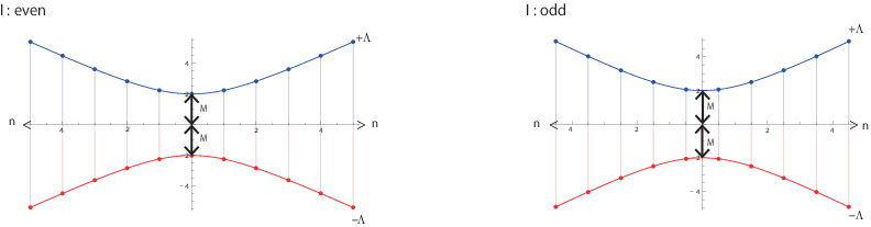
The corresponding degeneracies are summarized in Appendix C. Notice that the minimum value is not zero, but λn=0−(s=±1/2)2=14.{\lambda^{-}_{n=0}(s=\pm 1/2)}^{2}=\frac{1}{4}.

In the limit I→0I\rightarrow 0, the former representation [n,I2+12,±12]S​O​(2​k)|I=0=[n,12,±12]S​O​(2​k)[n,\frac{I}{2}+\frac{1}{2},\pm\frac{1}{2}]_{SO(2k)}|_{I=0}=[{n,\frac{1}{2},\pm\frac{1}{2}}]_{SO(2k)} gives the spectrum of the free spinor particle on S2​k−1S^{2k-1}:2121 21 For each of the eigenvalues (126), +(n+k−12)+(n+k-\frac{1}{2}) and −(n+k−12)-(n+k-\frac{1}{2}), the corresponding degeneracy is equally given by d​[n,1/2,1/2]S​O​(2​k)=2k−1​(n+2​k−2n)​(n=0,1,2,⋯)d[{n,{1}/{2}},{1}/{2}]_{SO(2k)}=2^{k-1}\begin{pmatrix}n+2k-2\\ n\end{pmatrix}~~~(n=0,1,2,\cdots) (125) which reproduces the known results of the free Dirac operator on S2​k−1S^{2k-1} (see Ref.[54] for instance).

±λn+(±1/2)⟶I→0−i∇=±(n+k−12),\pm\lambda^{+}_{n}(\pm 1/2)~\overset{I\rightarrow 0}{\longrightarrow}~-i\mathrlap{\not{\phantom{\nabla}}}\nabla=\pm(n+k-\frac{1}{2}), (126)

while the latter representation [n,I2−12,±12]S​O​(2​k)[n,\frac{I}{2}-\frac{1}{2},\pm\frac{1}{2}]_{SO(2k)} is not well defined, and then ±λn−(s=±1/2)\pm\lambda^{-}_{n}(s=\pm 1/2) do not have their counterparts in the spectrum of the free Dirac operator.

5.3 Total degeneracy of 00th Landau level revisited

For n=0n=0, λn−​(s)2{\lambda_{n}^{-}(s)}^{2} (117) takes a very simple form:

λn=0−​(s)2=s2,{\lambda_{n=0}^{-}(s)}^{2}=s^{2}, (127)

with degeneracy

2​(1−δs,0)​d​[0,I2−12,s]S​O​(2​k)+δs,0​d​[0,I2−12,0]S​O​(2​k)2(1-\delta_{s,0})~d[0,\frac{I}{2}-\frac{1}{2},s]_{SO(2k)}+\delta_{s,0}~d[0,\frac{I}{2}-\frac{1}{2},0]_{SO(2k)} (128)

where

d​[0,I2−12,s]S​O​(2​k)=∏j=1k−1(I+2​j−1)2−4​s2(2​j)2​∏l=1k−2∏j=1k−l−1I+2​l+j−12​l+j.d[0,\frac{I}{2}-\frac{1}{2},s]_{SO(2k)}=\prod_{j=1}^{k-1}\frac{(I+2j-1)^{2}-4s^{2}}{(2j)^{2}}\prod_{l=1}^{k-2}\prod_{j=1}^{k-l-1}\frac{I+2l+j-1}{2l+j}. (129)

Then we have

total dimension of the 00th Landau level
=2​∑s>0I2−12d​[0,I2−12,s]S​O​(2​k)​(+d​[0,I2−12,0]S​O​(2​k))=∑s=−I2+12I2−12d​[0,I2−12,s]S​O​(2​k)\displaystyle=2\sum_{s>0}^{\frac{I}{2}-\frac{1}{2}}d[0,\frac{I}{2}-\frac{1}{2},s]_{SO(2k)}~\biggl(+~d[0,\frac{I}{2}-\frac{1}{2},0]_{SO(2k)}\biggr)=\sum_{s=-\frac{I}{2}+\frac{1}{2}}^{\frac{I}{2}-\frac{1}{2}}d[0,\frac{I}{2}-\frac{1}{2},s]_{SO(2k)}
=νk​(I),\displaystyle=\nu_{k}(I), (130)

where Eq.(63) was used in the last equation. Zero-mode contribution ()(~~) on the second equation exists when II is odd. We will explain a differential topology origin behind this relation. First notice, since d​[0,I2−12]S​O​(2​k+1)d[0,\frac{I}{2}-\frac{1}{2}]_{SO(2k+1)} denotes the 0-mode degeneracy of the 2​k2kD relativistic Landau model, i.e.i.e., the index of the Dirac-Landau operator on S2​kS^{2k}, the dimensional ladder between 2​k2k and (2​k−1)(2k-1)D (87) can be rewritten as

∑s=−I2+12I2−12d​[0,I2−12,s]S​O​(2​k)=Ind​[−i​​DS​O​(2​k+1)].\sum_{s=-\frac{I}{2}+\frac{1}{2}}^{\frac{I}{2}-\frac{1}{2}}d[0,\frac{I}{2}-\frac{1}{2},s]_{SO(2k)}=\text{Ind}[-i\mathrlap{\not{\phantom{D}}}D_{SO(2k+1)}]. (131)

Second, we find that the Atiyah-Singer index theorem tells2222 22 On general spin manifold without boundary, the Atiyah-Singer theorem is given by Ind​(−i​​D)=∫MA^​(R)⋅c​h​(F),\text{Ind}(-i\mathrlap{\not{\phantom{D}}}D)=\int_{M}\hat{A}(R)\cdot ch(F), (132) where c​h​(F)ch(F) denotes the Chern number density and A^​(R)\hat{A}(R) represents the Dirac-genus given by the polynomials of the Pontryagin class: A^​(R)=1−124​p1​(R)+15760​(7​p1​(R)2−4​p2​(R))+⋯.\hat{A}(R)=1-\frac{1}{24}p_{1}(R)+\frac{1}{5760}(7{p_{1}(R)}^{2}-4p_{2}(R))+\cdots. (133) For spheres, the Pontryagin class is identically zero, and so the Dirac-genus becomes trivial. Consequently for S2​kS^{2k}, the index of the Dirac operator is determined solely by the gauge bundle topology: Ind​(−i​​D)=∫S2​kc​h​(F)=ck.\text{Ind}(-i\mathrlap{\not{\phantom{D}}}D)=\int_{S^{2k}}ch(F)=c_{k}. (134)

Ind​[−i​​DS​O​(2​k+1)]=ck​(I),\text{Ind}[-i\mathrlap{\not{\phantom{D}}}D_{SO(2k+1)}]=c_{k}(I), (135)

where ckc_{k} denotes the kkth Chern number of the S​O​(2​k)SO(2k) monopole charge. For the 2​k2kD Landau models, Eq.(135) can be verified explicitly [8]. Third, from the fibre-bundle theory, the non-trivial gauge topology on 2​k2k-sphere is evaluated by the winding number (60) from the transition function on the equator S2​k−1S^{2k-1}:

ck​(I)=νk​(I).c_{k}(I)=\nu_{k}(I). (136)

See Appendix D about a general proof of Eq.(136). In the present case, we can explicitly verify Eq.(136) as follows. Using the formula of d​[0,I2,s]S​O​(2​k−2)d[0,\frac{I}{2},s]_{SO(2k-2)} (53), we perform the the summation of the winding number (61) to have

νk​(I)=12k−1​(I+2​k−4)!!(2​k−3)!!​I!!​∑s=−I2I2(2​s)2​d​[0,I2,s]S​O​(2​k−2)=∏l=1k∏i=1lI+l+i−2l+i−2=d​[0,I−12]S​O​(2​k+1),\nu_{k}(I)=\frac{1}{2^{k-1}}\frac{(I+2k-4)!!}{(2k-3)!!I!!}\sum_{s=-\frac{I}{2}}^{\frac{I}{2}}(2s)^{2}d[0,\frac{I}{2},s]_{SO(2k-2)}=\prod_{l=1}^{k}\prod_{i=1}^{l}\frac{I+l+i-2}{l+i-2}=d[0,\frac{I-1}{2}]_{SO(2k+1)}, (137)

where d​[0,I2]S​O​(2​k+1)d[0,\frac{I}{2}]_{SO(2k+1)} is defined by Eq.(86). In Ref.[8], we showed d​[0,I−12]S​O​(2​k+1)=ck​(I)d[0,\frac{I-1}{2}]_{SO(2k+1)}=c_{k}(I), and then

ck​(I)=d​[0,I−12]S​O​(2​k+1)=νk​(I).c_{k}(I)=d[0,\frac{I-1}{2}]_{SO(2k+1)}=\nu_{k}(I). (138)

Finally, from Eq.(131), (135) and (136), we obtain the sequence

total dim. of odd D LLL​⟹dim. ladder (131)​Ind​[−i​​D]even D​⟹AS index theorem (135)​c​⟹fibre-bundle theory (136)​ν,\!\!\!\!\!\!\text{total dim. of odd D LLL}\overset{\text{dim. ladder (\ref{fromfuzzysphererel})}}{\Longrightarrow}~\text{Ind}[-i\mathrlap{\not{\phantom{D}}}D]_{\text{even D}}~\overset{\text{AS index theorem (\ref{indextheoremndc})}}{\Longrightarrow}~c~\overset{\text{fibre-bundle theory (\ref{candwindingrelation})}}{\Longrightarrow}~\nu, (139)

which verifies Eq.(130) after all. However, there is one speck in the above discussions. As for the dimensional ladder (131), we utilized specific properties of the Landau models, while the other processes of the sequence depend on general arguments of differential topology, such as Atiyah-Singer index theorem and fibre-bundle theory. We will reconsider the dimensional ladder and show that the dimensional ladder can also be understood from a differential topology point of view. In Sec.6, the total dimension of the 0th Landau level is shown to be equal to the spectral flow:

∑sd​[0,I2−12,s]S​O​(2​k)=−spectral flow.\sum_{s}d[0,\frac{I}{2}-\frac{1}{2},s]_{SO(2k)}=-~\text{spectral flow}. (140)

With Eq.(140) and the spectral flow argument of Atiyah-Patodi-Singer [47, 48, 49, 46]

−spectral flow=Ind​(−i​​D),-~\text{spectral flow}=\text{Ind}(-i\mathrlap{\not{\phantom{D}}}D), (141)

every process of the sequence (139) can be restated in the language of differential topology:

total dim. of odd D LLL​⟹APS spectral flow (141)​Ind​[−i​​D]even D​⟹AS index theorem (135)​c​⟹fibre-bundle theory (136)​ν.\!\!\!\!\!\!\text{total dim. of odd D LLL}\overset{\text{APS spectral flow (\ref{spectralflowAPS})}}{\Longrightarrow}~\text{Ind}[-i\mathrlap{\not{\phantom{D}}}D]_{\text{even D}}~\overset{\text{AS index theorem (\ref{indextheoremndc})}}{\Longrightarrow}~c~\overset{\text{fibre-bundle theory (\ref{candwindingrelation})}}{\Longrightarrow}~\nu. (142)

6 Ladder of Dimensions: Spectral Flow of Atiyah-Patodi-Singer

Let us discuss relations between the spectral flow argument of Atiyah-Patodi-Singer and the dimensional ladder between the 2​k2k and (2​k−1)(2k-1)D Landau models:

d​[0,I2]S​O​(2​k+1)=∑s=−I2I2d​[0,I2,s]S​O​(2​k).d[0,~\frac{I}{2}]_{SO(2k+1)}=\sum_{s=-\frac{I}{2}}^{\frac{I}{2}}d[0,~\frac{I}{2},~s]_{SO(2k)}. (143)

We demonstrate how Eq.(143) works in 1D and 2D relativistic Landau models and clarify relations to the spectral flow argument. For this purpose, we apply the Atiyah’s discussion [55] originally developed on torus S1⊗S1S^{1}\otimes S^{1} is applied to fuzzy two-sphere.2323 23 Also see Refs.[56, 57] for relations to quantum anomaly. In this section, we use the terminologies “lowest Landau level” and “0th Landau level” interchangeably.

6.1 2D and 1D relativistic Landau models

The massive Dirac-Landau operator on two-sphere is given by

−iDS2+Mσz=−iσx(∂θ−12tanθ2)−i1sin⁡θσy(∂ϕ−iAϕ)+Mσz,-i\mathrlap{\not{\phantom{D}}}D_{S^{2}}+M\sigma_{z}=-i\sigma_{x}(\partial_{\theta}-\frac{1}{2}\tan\frac{\theta}{2})-i\frac{1}{\sin\theta}\sigma_{y}(\partial_{\phi}-iA_{\phi})+M\sigma_{z}, (144)

where θ\theta and ϕ\phi represent the standard polar coordinates, 0≤θ<π0\leq\theta<\pi, 0≤ϕ<2​π0\leq\phi<2\pi, and AϕA_{\phi} denotes the monopole gauge field

A=Aϕ​d​ϕ=I2​(1−cos⁡θ)​d​ϕ.A=A_{\phi}d\phi=\frac{I}{2}(1-\cos\theta)d\phi. (145)

We omit the spin connection part to deduce a massive 1D Dirac-Landau operator from Eq.(144):

−iDS1+Mσz=−iσy(∂ϕ−iAϕ)+Mσz=(M−∂ϕ+iAϕ∂ϕ−iAϕ−M)-i\mathrlap{\not{\phantom{D}}}D_{S^{1}}+M\sigma_{z}=-i\sigma_{y}(\partial_{\phi}-iA_{\phi})+M\sigma_{z}\\ =\begin{pmatrix}M&-\partial_{\phi}+iA_{\phi}\\ \partial_{\phi}-iA_{\phi}&-M\end{pmatrix}

that respects the chiral symmetry:

{σx,−i​​DS1+M​σz}=0.\{\sigma_{x},-i\mathrlap{\not{\phantom{D}}}D_{S^{1}}+M\sigma_{z}\}=0. (146)

(−i​​DS1+M​σz-i\mathrlap{\not{\phantom{D}}}D_{S^{1}}+M\sigma_{z} denotes a 1D chiral topological insulator Hamiltonian.2424 24 Without the gauge field, Eq.(6.1) is reduced to the Jackiw-Rebbi Hamiltonian used for the low energy description of polyacetylene [59].) The 1D Dirac-Landau operator −i​​DS1-i\mathrlap{\not{\phantom{D}}}D_{S^{1}}

−i​​DS1=−i​σy​DS1=(0−DS1DS10)-i\mathrlap{\not{\phantom{D}}}D_{S^{1}}=-i\sigma_{y}D_{S^{1}}=\begin{pmatrix}0&-D_{S^{1}}\\ D_{S^{1}}&0\end{pmatrix} (147)

consists of two copies of the 1D Weyl-Landau operator

−iDS1=−i∂ϕ−Aϕ(θ),-iD_{S^{1}}=-i\partial_{\phi}-A_{\phi}^{(\theta)}, (148)

with

Aϕ(θ)=I2​(1−cos⁡θ).A^{(\theta)}_{\phi}=\frac{I}{2}(1-\cos\theta). (149)

Notice that in the 1D Weyl-Landau operator (148), θ\theta is no longer a coordinate but denotes an external parameter to tune the magnitude of the gauge field. While magnetic field is constant on the surface of the two-sphere, Eq.(148) describes the 1D Weyl operator with the magnetic flux at the center of S1S^{1} (Fig.2). The magnitude of the magnetic flux is given by

Φ(θ)=∮d​ϕ​Aϕ(θ)=2​π​Aϕ(θ)=π​I​(1−cos⁡θ),\Phi^{(\theta)}=\oint d\phi A^{(\theta)}_{\phi}=2\pi A^{(\theta)}_{\phi}=\pi I(1-\cos\theta), (150)

which monotonically increases from 00 to 2​π​I2\pi I as the parameter θ\theta changes from θ=0\theta=0 to π\pi.

Refer to caption
Figure 2: 1D Landau models as latitudes of the 2D Landau model.

6.1.1 Atiyah-Singer index theorem

There are not a few literatures about the non-relativistic/relativistic Landau problem on S2S^{2} (see Ref.[58] for instance). In the non-relativistic case, the lowest Landau level degeneracy is given by

dLLL2​D​(I2)=d​[0,I2]S​O​(3)=I+1,d_{\text{LLL}}^{2\text{D}}(\frac{I}{2})=d[0,\frac{I}{2}]_{SO(3)}=I+1, (151)

and the lowest Landau level basis states are the eigenstates of Xz=2I​LzX_{z}=\frac{2}{I}L_{z} with the eigenvalues

Xz=1−2I​m(m=0,1,2,⋯,I).X_{z}=1-\frac{2}{I}m~~~~~(m=0,1,2,\cdots,I). (152)

In other words, the lowest Landau level basis states correspond to the latitudes with the azimuthal angles θm\theta_{m}:

cos⁡θm=1−2I​m.\cos\theta_{m}=1-\frac{2}{I}m. (153)

The zero-mode degeneracy of the Dirac-Landau operator is obtained from the lowest Landau level degeneracy (151) with the replacement I2→I2−12\frac{I}{2}~\rightarrow~\frac{I}{2}-\frac{1}{2}, and the index of the Dirac-Landau operator is given by

Ind​(−i​​DS2)=dLLL2​D​(I2−12)=I.\text{Ind}(-i\mathrlap{\not{\phantom{D}}}D_{S^{2}})=d_{\text{LLL}}^{2\text{D}}(\frac{I}{2}-\frac{1}{2})=I. (154)

Meanwhile, the 1st Chern number of the monopole bundle is obtained as

c1​(g)=12​π​∫S2F=I.c_{1}(g)=\frac{1}{2\pi}\int_{S^{2}}F=I. (155)

Their equality manifests the Atiyah-Singer index theorem:

Ind​(−i​​DS2)=c1.\text{Ind}(-i\mathrlap{\not{\phantom{D}}}D_{S^{2}})=c_{1}. (156)

6.1.2 Spectral flow argument

Next let us consider the 1D Weyl-Landau model. With the magnetic flux Φ(θ)\Phi^{(\theta)} (150), the 1D Weyl-Landau operator is represented as

−iDS1=−i(∂ϕ−i12​πΦ(θ))=Lϕ,-iD_{S^{1}}=-i(\partial_{\phi}-i\frac{1}{2\pi}\Phi^{(\theta)})=L_{\phi}, (157)

which is simply the covariant derivative in ϕ\phi-direction or the covariant angular momentum, LϕL_{\phi}. Intuitively, the flux insertion brings the counter-propagating angular momentum along ϕ\phi direction (Fig.3).

Refer to caption
Figure 3: The flux insertion reduces the particle angular momentum due to the associated counter-propagating gauge field.

Since θ\theta is a continuum variable, the magnitude of the flux Φ(θ)=π​I​(1−cos⁡θ)\Phi^{(\theta)}=\pi I(1-\cos\theta), is not generally quantized unlike the monopole charge. However, with respect to the latitudes (153), the magnetic flux (150) is quantized as a multiple of unit flux:

Φ(θm)=2​π​m(m=0,1,2,⋯,I).\Phi^{(\theta_{m})}=2\pi m~~~~(m=0,1,2,\cdots,I). (158)

Thus by embedding, the magnetic charges of the odd D Landau models become quantized.

We solve the eigenvalue problem of the Weyl-Landau operator,

−i​DS1​ψn​(ϕ)=λn(θ)​ψn​(ϕ).-iD_{S^{1}}\psi_{n}(\phi)=\lambda_{n}^{(\theta)}\psi_{n}(\phi). (159)

Due to the periodic boundary condition, the eigenfunctions are obtained as

ψn​(ϕ)=12​π​ei​n​ϕ(n=0,±1,±2,⋯),\psi_{n}(\phi)=\frac{1}{\sqrt{2\pi}}e^{in\phi}~~~~~~~(n=0,\pm 1,\pm 2,\cdots), (160)

with the eigenvalues

λn(θ)=n−12​π​Φ(θ)=n−I2​(1−cos⁡θ).\lambda_{n}^{(\theta)}=n-\frac{1}{2\pi}\Phi^{(\theta)}=n-\frac{I}{2}(1-\cos\theta). (161)

The 1D Weyl-Landau model on the latitude (153) takes the energy eigenvalues

λn(θm)=n−m.\lambda_{n}^{(\theta_{m})}=n-m. (162)

When θ\theta changes from 00 to π\pi (or the magnetic flux Φ(θ)\Phi^{(\theta)} increases adiabatically from 00 to 2​π​I2\pi I), the spectrum evolves from nn to (n−I)(n-I) according to Eq.(161) (Fig.4).

Refer to caption
Figure 4: Evolving eigenvalues (161) during the process from θ=0\theta=0 to θ=π\theta=\pi with respect to I/2=1/2,1,3/2I/2={1}/{2},1,{3}/{2} from left to right. The eigenvalues cross the zero-energy (the red horizontal line) II times at the points indicated by the red filled circles, the number of which is the definition of the spectral flow. Since each Landau level reduces its energy by II during the process, the spectral flow is equal to the descent of energy level (the length of the purple down-arrow).

The flux insertion brings the counter-propagating gauge field during the process, and the particle on S1S^{1} reduces its angular momentum and travels down from the nnth circle to the (n−I)(n-I)th inner circle. Since the energy transition of 1D Landau model is equal to the number of the points at which the evolving eigenvalues cross the zero-energy horizontal line (Fig.4), we find that II is equal to (the minus of) the spectral flow:2525 25 The sign of the spectral flow is taken so that each positive/negative eigenvalue that becomes negative/positive contributes -1/+1 to the spectral flow counting.

−spectral flow=I.-~\text{spectral flow}=I. (163)

Recall that II was the index of the 2D Dirac-Landau operator (154). Then we have

Ind​(−i​​D)=−spectral flow,\text{Ind}(-i\mathrlap{\not{\phantom{D}}}D)=-~\text{spectral flow}, (164)

which manifests the spectral flow argument of Atiyah-Patodi-Singer.

6.2 Dimensional ladder of non-commutative geometry

In the above, we have seen the validity of the spectral flow argument in the context of the low dimensional Landau models, while in the following we will show that the spectral flow argument generally guarantees the dimensional ladder of the Landau models (143). The spectral flow indicates the number of points at which the evolving eigenstates cross the zero-energy. In view of the 1D Landau models, each crossing point corresponds to the lowest Landau level of the Landau model with different magnetic flux. Concretely, the mmth crossing point corresponds to the lowest Landau level of the Weyl-Landau model (157) with flux Φ(θm)=2​π​m\Phi^{(\theta_{m})}=2\pi m (Fig.4). Since the spectral flow indicates the number of the crossing points, the spectral flow is equal to the total number of the lowest Landau level states of II 1D Weyl-Landau models with Φ(θm)=2​π​m\Phi^{(\theta_{m})}=2\pi m (m=1,2,⋯,I)(m=1,2,\cdots,I):

−spectral flow=∑m=1IdLLL1​D​(m),-~\text{spectral flow}=\sum_{m=1}^{I}d_{\text{LLL}}^{1\text{D}}(m), (165)

where dLLL1​D​(m)d_{\text{LLL}}^{1\text{D}}(m) denotes the lowest Landau level degeneracy of the Weyl-Landau model with Φ(θm)\Phi^{(\theta_{m})}, and in the present case, obviously dLLL1​D​(m)=1d_{\text{LLL}}^{1\text{D}}(m)=1. Besides, the sum of the lowest Landau level states of the II Weyl-Landau models can be given by the sum of the states in different energy levels of a 𝑠𝑖𝑛𝑔𝑙𝑒\it{single} Weyl-Landau model. Notice that the lowest Landau level of the Weyl-Landau model for mm and s(=m−I2−12)s(=m-\frac{I}{2}-\frac{1}{2})th level of the Weyl-Landau model with Φ(θm=I/2−1/2)=π⁡(I−1)\Phi^{(\theta_{m={I}/{2}-{1}/{2}})}=\pi(I-1) are on the same evolving eigenvalue curve (see Fig.5):

dLLL1​D​(m)=ds=m−I2−121​D​(I2−12),d_{\text{LLL}}^{1\text{D}}(m)=d^{1\text{D}}_{s=m-\frac{I}{2}-\frac{1}{2}}(\frac{I}{2}-\frac{1}{2}), (166)

where ds1​D​(I2−12)d^{1\text{D}}_{s}(\frac{I}{2}-\frac{1}{2}) denotes the ssth level degeneracy of the Weyl-Landau model with flux Φ/(2​π)=I2−12\Phi/(2\pi)=\frac{I}{2}-\frac{1}{2}.

Refer to caption
Figure 5: Evolving eigenvalues of the 1D Weyl-Landau operator for I=3{I}={3}. The intersections (blue circles) between the blue vertical line and the energy curves represent the s(=−1,0,1)s(=-1,0,1)th levels of the Weyl-Landau operator with Φ(θm=I2−12)=π⁡(I−1)\Phi^{(\theta_{m=\frac{I}{2}-\frac{1}{2}})}=\pi(I-1). The intersections (red filled circles) between the zero-energy horizontal line and the energy curves indicate the lowest Landau levels of the Weyl-Landau models with Φ(θm=1,2,⋯,I)=2​π,4​π,⋯,2​π​I\Phi^{(\theta_{m=1,2,\cdots,I})}=2\pi,4\pi,\cdots,2\pi I. The blue circle and the red filled one on same eigenvalue curve are related by s=m−I2−12s=m-\frac{I}{2}-\frac{1}{2}.

Hence, the spectral flow (165) can be expressed by the sum of the level degeneracies of the single Weyl-Landau model with Φ/(2​π)=I2−12\Phi/(2\pi)=\frac{I}{2}-\frac{1}{2},

−spectral flow=∑s=−I2+12I2−12ds1​D​(I2−12).-~\text{spectral flow}=\sum_{s=-\frac{I}{2}+\frac{1}{2}}^{\frac{I}{2}-\frac{1}{2}}d^{1\text{D}}_{s}(\frac{I}{2}-\frac{1}{2}). (167)

This relation is naturally generalized to higher dimensions as

−spectral flow=∑s=−I2+12I2−12ds(2​k−1)​D​(I2−12)=∑s=−I2+12I2−12d​[0,I2−12,s]S​O​(2​k),-~\text{spectral flow}=\sum_{s=-\frac{I}{2}+\frac{1}{2}}^{\frac{I}{2}-\frac{1}{2}}d^{(2k-1)\text{D}}_{s}(\frac{I}{2}-\frac{1}{2})=\sum_{s=-\frac{I}{2}+\frac{1}{2}}^{\frac{I}{2}-\frac{1}{2}}d[0,\frac{I}{2}-\frac{1}{2},s]_{SO(2k)}, (168)

which is the sought formula (140) that relates the odd D Landau level degeneracies and the spectral flow. Besides, the spectral flow argument tells

Ind​(−i​​D)=−spectral flow,\text{Ind}(-i\mathrlap{\not{\phantom{D}}}D)=-~\text{spectral flow}, (169)

and we eventually have

d​[0,I2−12]S​O​(2​k+1)=Ind​(−i​​D)=−spectral flow=∑s=−I2+12I2−12d​[0,I2−12,s]S​O​(2​k).d[0,\frac{I}{2}-\frac{1}{2}]_{SO(2k+1)}=\text{Ind}(-i\mathrlap{\not{\phantom{D}}}D)=-~\text{spectral flow}=\sum_{s=-\frac{I}{2}+\frac{1}{2}}^{\frac{I}{2}-\frac{1}{2}}d[0,\frac{I}{2}-\frac{1}{2},s]_{SO(2k)}. (170)

This is the very formula of the dimensional ladder (143). As discussed above, the spectral flow argument of Atiyah-Patodi-Singer guarantees the validity of the dimensional ladder of the Landau models. In other words, the dimensional ladder of non-commutative geometry can thus find its origin in the differential topology.

We recapitulate the above discussions with the 1D and 2D Landau models. From the two-sphere point of view, θ\theta is the azimuthal angle, and the change of θ\theta from 00 to π\pi corresponds to a sweep on S2S^{2} from north pole to the south pole transversing II latitudes, which is the dimension of the 2D relativistic lowest Landau level, dLLL2​D​(I2−12)d_{\text{LLL}}^{2\text{D}}(\frac{I}{2}-\frac{1}{2}). During the sweep, the magnetic flux changes from 00 to 2​π​I2\pi I, and then each energy level of the 1D Weyl-Landau model decreases by II that is the spectral flow. The spectral flow is equal to the total dimension of the corresponding 1D Landau levels. We can thus restate Eq.(170) as

2D LLL dim.⇒sweep on (fuzzy) two-sphere⇒spectral flow⇒total dim. of 1D LLs.\text{2D LLL dim.}\Rightarrow\text{sweep on (fuzzy) two-sphere}\Rightarrow\text{spectral flow}\Rightarrow\text{total dim. of 1D LLs}. (171)

Fig.6 shows (171) pictorially.

Refer to caption
Figure 6: An intuitive picture of the dimensional ladder (for I=2I=2). The third figure signifies 90∘ rotated figure of evolving eigenvalues.

7 BF Effective Field Theory

There arise (2​k−2)(2k-2)-branes as fundamental excitations in 2​k2kD quantum Hall effect, and a (4​k−1)(4k-1)D tensor Chern-Simons action is proposed for the description of such membranes [8]:

S=−e2​k−2∫4​k−1𝒞2​k−1𝒥2​k+κ2∫4​k−1𝒞2​k−1𝒢2​k,S=-e_{2k-2}\int_{4k-1}\mathcal{C}_{2k-1}\mathcal{J}_{2k}+\frac{\kappa}{2}\int_{4k-1}\mathcal{C}_{2k-1}\mathcal{G}_{2k}, (172)

where 𝒢2​k=d​𝒞2​k−1\mathcal{G}_{2k}=d\mathcal{C}_{2k-1}, 𝒥2​k\mathcal{J}_{2k} denotes the (2​k−2)(2k-2)-brane current, and κ\kappa stands for the Chern–Simons coupling constant,

κ=e2​k−22​π​1mk.\kappa=\frac{e_{2k-2}}{2\pi}\frac{1}{m^{k}}. (173)

mm represents an odd integer to specify the filling factor by ν2​k=1mk\nu_{2k}=\frac{1}{m^{k}}.2626 26 ν2​k\nu_{2k} has nothing to do with the winding number in Sec. 3. The tensor Chern–Simons action induces the tensor flux attachment to membrane and accounts for non-trivial linking of (2​k−2)(2k-2)-brane currents [60]. Let us consider similar field theory formulation for the odd D quantum Hall effect. As the (4​k−1)(4k-1)D tensor Chern–Simons action was used for the description of the 2​k2kD quantum Hall effect, one may be tempted to adopt (4​k−3)(4k-3)D tensor Chern-Simons action for the present odd D case, but the (4​k−3)(4k-3)D tensor Chern–Simons action identically vanishes: In (4​k−3)(4k-3)D, the tensor Chern–Simons field has to be even rank, but the Chern–Simon form of even rank tensor becomes

𝒞2​k−2∧d​𝒞2​k−2=−d​𝒞2​k−2∧𝒞2​k−2=−𝒞2​k−2∧d​𝒞2​k−2=0\mathcal{C}_{2k-2}\wedge d\mathcal{C}_{2k-2}=-d\mathcal{C}_{2k-2}\wedge\mathcal{C}_{2k-2}=-\mathcal{C}_{2k-2}\wedge d\mathcal{C}_{2k-2}=0 (174)

on closed manifolds. The use of (4​k−3)(4k-3)D tensor Chern-Simons action is thus in vain.

Considering that the odd D quantum Hall effect is embedded in one-dimension higher quantum Hall effect, a natural idea to construct effective field theory for the odd D quantum Hall effect will be to use one-dimension reduction of the tensor Chern–Simons theory for the even D. Such theory is a tensor type BF theory in (4​k−2)(4k-2)D that we will pursue in this section. (4​k−2)(4k-2)D space–time is the emergent space–time for (2​k−1)(2k-1)D quantum Hall effect as (4​k−1)(4k-1)D for 2​k2kD quantum Hall effect (Table 2). BF theory is a topological field theory defined in arbitrary dimensions [61, 62, 63] and describes fractional statistics of extended objects. For instance in (3+1)(3+1)D, BF theory is used to describe the linking and fractional statistics [64, 65, 66, 67] between particle and vortex-string coupled to 2-rank antisymmetric tensor field [68]. We will make use of such properties of BF theory in (4​k−2)(4k-2)D space–time.

The original space-time D  2  4  6  8 10 12 14 16 18 ⋯\cdots
The emergent space-time D  2  6 10 14 18 22 26 30 34 ⋯\cdots
Table 2: The emergent (4​k−2)(4k-2)D space-time for the (2​k−1)(2k-1)D quantum Hall effect.

7.1 BF theory as a reduced Chern-Simons theory

Accompanied with one dimension reduction of the (4​k−1)(4k-1)D Chern-Simons action, the (2​k−1)(2k-1) tensor Chern-Simons field and (2​k−2)(2k-2)-brane current 𝒥2​k\mathcal{J}_{2k} in Eq.(172) are decomposed as

𝒞2​k−1=C2​k−1+C2​k−2​d​x4​k−2,\displaystyle\mathcal{C}_{2k-1}=C_{2k-1}+C_{2k-2}dx^{4k-2},
𝒥2​k=J2​k−1∧d​x4​k−2+J2​k.\displaystyle\mathcal{J}_{2k}=J_{2k-1}\wedge dx^{4k-2}+J_{2k}. (175)

In component representation, Eq.(7.1) is expressed as

Ca1a2⋯a2​k−1→Cμ1μ2⋯μ2​k−1,Cμ1μ2⋯μ2​k−2,4k−2,\displaystyle C_{a_{1}a_{2}\cdots a_{2k-1}}~\rightarrow~C_{\mu_{1}\mu_{2}\cdots\mu_{2k-1}},~C_{\mu_{1}\mu_{2}\cdots\mu_{2k-2},{4k-2}},
Ja1a2⋯a2​k−1→Jμ1μ2⋯μ2​k−1,Jμ1μ2⋯μ2​k−2,4k−2,\displaystyle J_{a_{1}a_{2}\cdots a_{2k-1}}~\rightarrow~J_{\mu_{1}\mu_{2}\cdots\mu_{2k-1}},~J_{\mu_{1}\mu_{2}\cdots\mu_{2k-2},{4k-2}}, (176)

with a1,a2,⋯,a2​k−1=0,1,2,⋯,4​k−2a_{1},a_{2},\cdots,a_{2k-1}=0,1,2,\cdots,4k-2 and μ1,μ2,⋯,μ2​k−1=0,1,2,⋯,4​k−3\mu_{1},\mu_{2},\cdots,\mu_{2k-1}=0,1,2,\cdots,4k-3. Here, C2​k−1C_{2k-1} and C2​k−2C_{2k-2} are taken to be independent on the compactified space coordinate x4​k−2x^{4k-2}. With S1S^{1}-compactification with radius RR, we derive the reduced Chern-Simons action in (4​k−2)(4k-2)D as2727 27 In component representation, the decomposition (7.1) is given as follows. With 𝒞2​k−1=1(2​k−1)!Ca1a2⋯a2​k−1dxa1dxa2⋯dxa2​k−1,\displaystyle\mathcal{C}_{2k-1}=\frac{1}{(2k-1)!}C_{a_{1}a_{2}\cdots a_{2k-1}}dx^{a_{1}}dx^{a_{2}}\cdots dx^{a_{2k-1}}, 𝒥2​k=1(2​k−1)!​(2​k)!ϵa1a2⋯a4​k−1Ja1a2⋯a2​k−1dxa2​kdxa2​k+1⋯dxa4​k−1,\displaystyle\mathcal{J}_{2k}=\frac{1}{(2k-1)!(2k)!}\epsilon^{a_{1}a_{2}\cdots a_{4k-1}}{J}_{a_{1}a_{2}\cdots a_{2k-1}}dx_{a_{2k}}dx_{a_{2k+1}}\cdots dx_{a_{4k-1}}, (177) we have C2​k−1=1(2​k−1)!Cμ1μ2⋯μ2​k−1dxμ1dxμ2⋯dxμ2​k−1,\displaystyle C_{2k-1}=\frac{1}{(2k-1)!}C_{\mu_{1}\mu_{2}\cdots\mu_{2k-1}}dx^{\mu_{1}}dx^{\mu_{2}}\cdots dx^{\mu_{2k-1}}, C2​k−2=1(2​k−2)!Cμ1μ2⋯μ2​k−2,4k−2dxμ1dxμ2⋯dxμ2​k−2,\displaystyle C_{2k-2}=\frac{1}{(2k-2)!}C_{\mu_{1}\mu_{2}\cdots\mu_{2k-2},4k-2}dx^{\mu_{1}}dx^{\mu_{2}}\cdots dx^{\mu_{2k-2}}, (178) and J2​k−1=1((2​k−1)!)2ϵμ1μ2⋯μ4​k−2Jμ1μ2⋯μ2​k−1dxμ2​k⋯dxμ4​k−2,\displaystyle J_{2k-1}=\frac{1}{((2k-1)!)^{2}}\epsilon^{\mu_{1}\mu_{2}\cdots\mu_{4k-2}}J_{\mu_{1}\mu_{2}\cdots\mu_{2k-1}}dx_{\mu_{2k}}\cdots dx_{\mu_{4k-2}}, J2​k=1(2​k)!​(2​k−2)!ϵμ1μ2⋯μ4​k−2Jμ1μ2⋯μ2​k−2,4k−2dxμ2​k−1⋯dxμ4​k−2.\displaystyle J_{2k}=\frac{1}{(2k)!(2k-2)!}\epsilon^{\mu_{1}\mu_{2}\cdots\mu_{4k-2}}J_{\mu_{1}\mu_{2}\cdots\mu_{2k-2},4k-2}dx_{\mu_{2k-1}}\cdots dx_{\mu_{4k-2}}. (179) The (4​k−2)(4k-2)D reduced Chern-Simons action (181) is expressed as S(4​k−2)​D=2​π​R(2​k−1)!​∫d4​k−2​x\displaystyle S_{(4k-2)\text{D}}=\frac{2\pi R}{(2k-1)!}\int d^{4k-2}x (−e2​k−2Cμ1μ2⋯μ2​k−1Jμ1μ2⋯μ2​k−1−e2​k−2(2k−1)Cμ1μ2⋯μ2​k−2Jμ1μ2⋯μ2​k−2\displaystyle\biggl(-e_{2k-2}C_{\mu_{1}\mu_{2}\cdots\mu_{2k-1}}J^{\mu_{1}\mu_{2}\cdots\mu_{2k-1}}-e_{2k-2}(2k-1)C_{\mu_{1}\mu_{2}\cdots\mu_{2k-2}}J^{\mu_{1}\mu_{2}\cdots\mu_{2k-2}} +κ(2​k−2)!ϵμ1μ2⋯μ4​k−2Cμ1μ2⋯μ2​k−1∂μ2​kCμ2​k+1⋯μ4​k−2)+(surface-term).\displaystyle+\frac{\kappa}{(2k-2)!}\epsilon^{\mu_{1}\mu_{2}\cdots\mu_{4k-2}}C_{\mu_{1}\mu_{2}\cdots\mu_{2k-1}}\partial_{\mu_{2k}}C_{\mu_{2k+1}\cdots\mu_{4k-2}}\biggr)+(\text{surface-term}). (180) :

S(4​k−2)​D\displaystyle S_{(4k-2)\text{D}} =−2πR⋅(e2​k−2∫4​k−2(C2​k−1J2​k−1+C2​k−2J2​k)−κ2∫4​k−2(C2​k−1G2​k−1+C2​k−2G2​k))\displaystyle=-2\pi R\cdot\biggl(e_{2k-2}\int_{4k-2}(C_{2k-1}J_{2k-1}+C_{2k-2}J_{2k})-\frac{\kappa}{2}\int_{4k-2}(C_{2k-1}G_{2k-1}+C_{2k-2}G_{2k})\biggr)
=−2πR⋅(e2​k−2∫4​k−2(C2​k−1J2​k−1+C2​k−2J2​k)−κ∫4​k−2C2​k−1dC2​k−2+(surface term)),\displaystyle=-2\pi R\cdot\biggl(e_{2k-2}\int_{4k-2}(C_{2k-1}J_{2k-1}+C_{2k-2}J_{2k})-{\kappa}\int_{4k-2}C_{2k-1}dC_{2k-2}+(\text{surface~term})\biggr), (181)

where

G2​k−1=d​C2​k−2,G2​k=d​C2​k−1.G_{2k-1}=dC_{2k-2},~~~~G_{2k}=dC_{2k-1}. (182)

The two tensor gauge fields, C2​k−1C_{2k-1} and C2​k−2C_{2k-2}, are coupled to different membranes with dimensions (2​k−2)(2k-2) and (2​k−3)(2k-3), and the membrane currents are given by J2​k−1J_{2k-1} and J2​kJ_{2k}. Thus there exist two kinds of membranes in odd dimensional quantum Hall effect. However, since both (2​k−2)(2k-2) and (2​k−3)(2k-3)-branes originate from (2​k−2)(2k-2)-brane in one-dimension higher space, their coupling constants to the Chern-Simons fields are equally given by (2​π​R)​e2​k−2(2\pi R)e_{2k-2}. From Eq.(181), the equations of motion are derived as

J2​k−1=κe2​k−2​G2​k−1,J2​k=−κe2​k−2​G2​k.J_{2k-1}=\frac{\kappa}{e_{2k-2}}G_{2k-1},~~~~~J_{2k}=-\frac{\kappa}{e_{2k-2}}G_{2k}. (183)

As component equations, Eq.(183) becomes

Ji1⋯i2​k−20=κe2​k−2Bi1⋯i2​k−2,Ji1⋯i2​k−30=κe2​k−2Bi1⋯i2​k−3,J^{i_{1}\cdots i_{2k-2}0}=\frac{\kappa}{e_{2k-2}}B^{i_{1}\cdots i_{2k-2}},~~~~J^{i_{1}\cdots i_{2k-3}0}=\frac{\kappa}{e_{2k-2}}B^{i_{1}\cdots i_{2k-3}}, (184)

and

Ji1⋯i2​k−1=−1(2​k−2)!κe2​k−2ϵi1⋯i4​k−3Ei2​k⋯i4​k−3,Ji1⋯i2​k−2=1(2​k−1)!κe2​k−2ϵi1⋯i4​k−3Ei2​k−1⋯i4​k−3.J^{i_{1}\cdots i_{2k-1}}=-\frac{1}{(2k-2)!}\frac{\kappa}{e_{2k-2}}\epsilon^{i_{1}\cdots i_{4k-3}}E_{i_{2k}\cdots i_{4k-3}},~~~~J^{i_{1}\cdots i_{2k-2}}=\frac{1}{(2k-1)!}\frac{\kappa}{e_{2k-2}}\epsilon^{i_{1}\cdots i_{4k-3}}E_{i_{2k-1}\cdots i_{4k-3}}. (185)

Here, Bi1⋯i2​k−2≡−1(2​k−1)!ϵi1⋯i4​k−3Gi2​k−1⋯i4​k−3B^{i_{1}\cdots i_{2k-2}}\equiv-\frac{1}{(2k-1)!}\epsilon^{i_{1}\cdots i_{4k-3}}G_{i_{2k-1}\cdots i_{4k-3}}, Bi1⋯i2​k−3≡−1(2​k)!ϵi1⋯i4​k−3Gi2​k−2⋯i4​k−3B^{i_{1}\cdots i_{2k-3}}\equiv-\frac{1}{(2k)!}\epsilon^{i_{1}\cdots i_{4k-3}}G_{i_{2k-2}\cdots i_{4k-3}}, Ei1⋯i2​k−2≡Gi1⋯i2​k−20E_{i_{1}\cdots i_{2k-2}}\equiv G_{i_{1}\cdots i_{2k-2}0} and Ei1⋯i2​k−1≡Gi1⋯i2​k−10E_{i_{1}\cdots i_{2k-1}}\equiv G_{i_{1}\cdots i_{2k-1}0}. Eq.(184) signifies a generalized flux attachment to membranes, and similarly Eq.(185) a generalized Hall effect. Either (2​k−2)(2k-2)-brane or (2​k−3)(2k-3)-brane current does not solely satisfy the Hall effect, Ei1⋯i2​k−1Ji1⋯i2​k−1≠0E_{i_{1}\cdots i_{2k-1}}J^{i_{1}\cdots i_{2k-1}}\neq 0, Ei1⋯i2​k−2Ji1⋯i2​k−2≠0E_{i_{1}\cdots i_{2k-2}}J^{i_{1}\cdots i_{2k-2}}\neq 0, but their sum does:

Ei1⋯i2​k−1Ji1⋯i2​k−1+(2k−1)Ei1⋯i2​k−2Ji1⋯i2​k−2=0.E_{i_{1}\cdots i_{2k-1}}J^{i_{1}\cdots i_{2k-1}}+(2k-1)E_{i_{1}\cdots i_{2k-2}}J^{i_{1}\cdots i_{2k-2}}=0. (186)

These properties reflect the fact that the present BF action originates from a single Chern-Simons action in one dimension higher space.

7.2 Effective action for membranes and linking number

The present BF theory in (4​k−2)(4k-2)D space-time accommodates the (2​k−2)(2k-2) and (2​k−3)(2k-3)-branes with unoccupied two-dimensional space (Table.3).

Dim.    0    1    2 ⋯\cdots 2​k−22k-2 2​k−12k-1 2​k−22k-2 ⋯\cdots 4​k−54k-5 4​k−44k-4 4​k−34k-3
M2​k−2M_{2k-2} ∘\circ ∘\circ ∘\circ ⋯\cdots ∘\circ −- −- ⋯\cdots −- −- −-
M2​k−3M_{2k-3} ∘\circ −- −- ⋯\cdots −- ∘\circ ∘\circ ⋯\cdots ∘\circ −- −-
Table 3: Two non-overlapping (2​k−2)(2k-2) and (2​k−3)(2k-3)-branes in (4​k−2)(4k-2)D space-time. From the co-dimension 2, the (2​k−2)(2k-2) and (2​k−3)(2k-3)-branes are regarded as two point particles.

In such two dimensions, (2​k−2)(2k-2) and (2​k−3)(2k-3)-branes are regarded as point-like objects, and the braiding of these objects is well-defined. In this sense, the membranes obey a generalized fractional statistics. With the use of Eq.(183), we can express the tensor fields by the associated membrane currents, and an effective membrane–membrane interaction can be derived from Eq.(181) as

Seff=2πR⋅e2​k−22κ∫d4​k−2x∫d4​k−2yϵμ1μ2⋯μ4​k−2Jμ1⋯μ2​k−1(x)∂μ2​k(1∂2)x,yJμ2​k+1⋯μ4​k−2(y).S_{\text{eff}}=2\pi R\cdot\frac{{e_{2k-2}}^{2}}{\kappa}\int d^{4k-2}x\int d^{4k-2}y~\epsilon^{\mu_{1}\mu_{2}\cdots\mu_{4k-2}}J_{\mu_{1}\cdots\mu_{2k-1}}(x)\partial_{\mu_{2k}}\biggl(\frac{1}{\partial^{2}}\biggr)_{x,y}J_{\mu_{2k+1}\cdots\mu_{4k-2}}(y). (187)

In the thin membrane limit (see Appendix E for details), the integral part becomes the linking number between the membrane trajectories,

L⁡(M2​k−2×S1,M2​k−3×S1)\displaystyle L(M_{2k-2}\times S^{1},M_{2k-3}\times S^{1}) =12​(2​k−1)!​π2​k−1∮M2​k−2×S1dxμ1⋯μ2​k−1\displaystyle=\frac{1}{2(2k-1)!\pi^{2k-1}}~\oint_{M_{2k-2}\times S^{1}}dx^{\mu_{1}\cdots\mu_{2k-1}}
×∮M2​k−3×S1dyμ2​k⋯μ4​k−3⋅1|x−y|4​k−2ϵμ1μ2⋯μ4​k−2(xμ4​k−2−yμ4​k−2),\displaystyle\times\oint_{M_{2k-3}\times S^{1}}dy^{\mu_{2k}\cdots\mu_{4k-3}}\cdot\frac{1}{|x-y|^{4k-2}}~\epsilon_{\mu_{1}\mu_{2}\cdots\mu_{4k-2}}(x_{\mu_{4k-2}}-y_{\mu_{4k-2}}), (188)

and the effective action (187) is reduced to

Seff=2​π​R⋅e2​k−22κ⋅L⁡(M2​k−2×S1,M2​k−3×S1).S_{\text{eff}}=2\pi R\cdot\frac{{e_{2k-2}}^{2}}{\kappa}\cdot L(M_{2k-2}\times S^{1},M_{2k-3}\times S^{1}). (189)

The integral part of Eq.(188) denotes the area of S4​k−3S^{4k-3} with coordinates xμ−yμ|x−y|\frac{x_{\mu}-y_{\mu}}{|x-y|} (Appendix E), and so the linking number (188) is equivalent to the winding number accompanied with

(M2​k−2×S1)×(M2​k−3×S1)⟶Sn−1.(M^{2k-2}\times S^{1})\times(M^{2k-3}\times S^{1})~~\longrightarrow~~S^{n-1}. (190)

When the membranes are spherical, we have

(S2​k−2×S1)×(S2​k−3×S1)⟶S4​k−3,(S^{2k-2}\times S^{1})\times(S^{2k-3}\times S^{1})~~\longrightarrow~~S^{4k-3}, (191)

indicating that the linking number is integer.

In the case that quantum Hall effect contains internal degrees of freedom [15], the BF theory is simply generalized to include KK matrix:

S(4​k−2)​D\displaystyle S_{{(4k-2)}\text{D}} =−2πR⋅(e2​k−2∫4​k−2(C2​k−1αJ2​k−1α+C2​k−2αJ2​kα)+12Kα​β∫4​k−2(C2​k−1αG2​k−1β+C2​k−2αG2​kβ)),\displaystyle=-2\pi R\cdot\biggl(e_{2k-2}\int_{4k-2}(C_{2k-1}^{\alpha}J_{2k-1}^{\alpha}+C_{2k-2}^{\alpha}J_{2k}^{\alpha})+\frac{1}{2}K_{\alpha\beta}\int_{4k-2}(C_{2k-1}^{\alpha}G_{2k-1}^{\beta}+C_{2k-2}^{\alpha}G_{2k}^{\beta})\biggr), (192)

and the effective action of the membrane-membrane interaction is derived as

Seff=2​π​R⋅ek−22​(1K)α​β​Lα​β,S_{\text{eff}}=2\pi R\cdot{e_{k-2}}^{2}\biggl(\frac{1}{K}\biggr)_{\alpha\beta}L^{\alpha\beta}, (193)

with

Lα​β≡L⁡(M2​k−2α×S1,M2​k−3β×S1).L^{\alpha\beta}\equiv L(M_{2k-2}^{\alpha}\times S^{1},M_{2k-3}^{\beta}\times S^{1}). (194)

8 Extended Dimensional Hierarchy

In 2​k2kD quantum Hall effect, the filling factor exhibits a hierarchical structure referred to as the dimensional hierarchy [8, 9]:

ν2​k=1m12​k​(k+1)=1m1m2⋯1mk\nu_{2k}=\frac{1}{m^{\frac{1}{2}k(k+1)}}=\frac{1}{m}\frac{1}{m^{2}}\cdots\frac{1}{m^{k}} (195)

or

ν2​k=1mk​ν2​k−2.\nu_{2k}=\frac{1}{m^{k}}\nu_{2k-2}. (196)

According to the Haldane-Halperin hierarchy [4, 69], in the usual 2D quantum Hall liquid, hierarchical nature of the filling factor is a reflection of new formations of incompressible liquids by quasi-particle condensation. Therefore, the dimensional hierarchy suggests “dimensional condensation” of membrane-like excitations: Low dimensional membranes condense to form incompressible liquid in two-dimension higher space, and the resulting higher D liquids also behave as membranes and condense again to form a new incompressible liquid in even higher dimensional space. Such condensation process repeatedly occurs from 0 to 2​k2kD, and consequently the filling factor bears a hierarchical structure in dimensions (195). The dimensional hierarchy can be understood by simple dimension counting. In 2​k2kD quantum Hall effect there are (2​k−2)(2k-2)-branes occupying an area ℓB2​k{\ell_{B}}^{2k} (ℓB=I/R)(\ell_{B}=\sqrt{I/R}), and the number of (2​k−2)(2k-2)-branes on 2​k2k-sphere is evaluated as

R2​kℓB2​k=Ik.\frac{R^{2k}}{{\ell_{B}}^{2k}}=I^{k}. (197)

Since the membrane condensation repeatedly occurs from 00-branes to (2​k−2)(2k-2)-branes, the total number of 0-branes on S2​kS^{2k} is

d2​k(I)≡I⋅I2⋯Ik=I12​k​(k+1).d_{2k}(I)\equiv I\cdot I^{2}\cdots I^{k}=I^{\frac{1}{2}k(k+1)}. (198)

The filling factor is scaled inversely in terms of the magnetic field (or the monopole charge), and then the scaling of the filling factor becomes Eq.(195). One may also see that Eq.(198) can be obtained from the lowest Landau level degeneracy of the Dirac-Landau operator, i.e.i.e., the Dirac operator index:

Ind ​(−i​​D)S​O​(2​k+1)=dS​O​(2​k+1)​[0,I2−12]=∏l=1k∏i=1lI+l+i−2l+i−1∼I12​k​(k+1).\text{Ind }(-i\mathrlap{\not{\phantom{D}}}D)_{SO(2k+1)}=d_{SO(2k+1)}[0,\frac{I}{2}-\frac{1}{2}]=\prod_{l=1}^{k}\prod_{i=1}^{l}\frac{I+l+i-2}{l+i-1}~\sim~I^{\frac{1}{2}k(k+1)}. (199)

Let us consider whether such dimensional hierarchy will occur in the odd D quantum Hall effects. Membranes on S2​k−1S^{2k-1} are supposed to occupy the area ℓB2​k−1{\ell_{B}}^{2k-1}, and similar dimension counting suggests that the number of the membranes would be

R2​k−1ℓB2​k−1=Ik−12,\frac{R^{2k-1}}{{\ell_{B}}^{2k-1}}=I^{k-\frac{1}{2}}, (200)

and the number of 0-branes would also be

I12⋅I32⋯Ik−12=I12​k2,I^{\frac{1}{2}}\cdot I^{\frac{3}{2}}\cdots I^{k-\frac{1}{2}}=I^{\frac{1}{2}k^{2}}, (201)

which however does not coincide with the sub-band degeneracy of the (2​k−1)(2k-1)D lowest Landau level:

dS​O​(2​k)​[0,I2−12,s]\displaystyle d_{SO(2k)}[0,\frac{I}{2}-\frac{1}{2},s] =∏j=1k−1(I+2​j−1)2−4​s2(2​j)2​∏l=1k−2∏j=1k−l−1I+2​l+j−12​l+j\displaystyle=\prod_{j=1}^{k-1}\frac{(I+2j-1)^{2}-4s^{2}}{(2j)^{2}}\prod_{l=1}^{k-2}\prod_{j=1}^{k-l-1}\frac{I+2l+j-1}{2l+j}
∼d2​k−1(I)≡I12​(k−1)​(k+2)(s<<I).\displaystyle\sim~d_{{2k-1}}(I)\equiv I^{\frac{1}{2}(k-1)(k+2)}~~~~~~~~~~(s<<I). (202)

The understanding of the scaling based on the simple dimensional analysis thus fails in the case of the odd D quantum Hall effects. However, Eq.(202) suggests the alternative scaling of the filling factor

ν2​k−1=1m12​(k−1)​(k+2),\nu_{2k-1}=\frac{1}{m^{\frac{1}{2}(k-1)(k+2)}}, (203)

which exhibits a hierarchical structure similar to the even D case (195):

1m12​(k−1)​(k+2)=1m21m3⋯1mk,\frac{1}{m^{\frac{1}{2}(k-1)(k+2)}}=\frac{1}{m^{2}}\frac{1}{m^{3}}\cdots\frac{1}{m^{k}}, (204)

or

ν2​k−1=1mk​ν2​k−3.\nu_{2k-1}=\frac{1}{m^{k}}\nu_{2k-3}. (205)

Therefore, the condensation mechanism is expected to work also in the odd D quantum Hall effect. Considering that (2​k−1)(2k-1)D quantum Hall effect is realized as a “subspace” of 2​k2kD quantum Hall effect, it is no wonder if similar mechanism may operate in odd D case.

From Eq.(195) and (203), we find the relationship between even D and odd D:

ν2​k=1m⋅ν2​k−1,\nu_{2k}=\frac{1}{m}\cdot\nu_{2k-1}, (206)

or

I⋅d2​k−1​(I)=d2​k​(I).I\cdot d_{{2k-1}}(I)=d_{2k}(I). (207)

Obviously, Eq.(207) is a manifestation of the dimensional ladder between (2​k−1)(2k-1) and 2​k2kD (93) discussed in Sec.4.2. From Eq.(196) and (206), another dimensional ladder between (2​k+1)(2k+1) and 2​k2kD is inferred as

ν2​k+1=1mk​ν2​k,\nu_{2k+1}=\frac{1}{m^{k}}\nu_{2k}, (208)

or

Ik⋅d2​k​(I)=d2​k+1​(I).I^{k}\cdot d_{2k}(I)=d_{2k+1}(I). (209)

This relation implies that IkI^{k} 2​k2k-branes or 2​k2kD quantum Hall liquids condense to form one-dimension higher (2​k+1)(2k+1)D quantum Hall liquid. Fig. 7 summarizes mutual relations among the higher D quantum Hall effects that we call the extended dimensional hierarchy.

Refer to caption
Figure 7: The extended dimensional hierarchy. The quantum Hall liquids in different dimensions are related by the web. See also the topological periodic table (Table 1) of A and AIII-class.

We add some comments on the relations to anomaly in relativistic quantum field theory and D-brane physics in string theory. The original dimensional hierarchy (196) was only for even D quantum Hall effects, which may correspond to the relationship between chiral anomaly and gauge anomaly in even dimensions [41, 42, 43, 44]. We have pointed out a new relation in dimensions of the quantum Hall effects (206) – the dimensional ladder between even and odd dimensions. This ladder is associated with the relationship between even D chiral anomaly and odd D parity anomaly [46]. Therefore, the extended dimensional hierarchy including the original hierarchy and ladder will be a counterpart of more general relationships among anomalies in arbitrary dimensions, such as Stora–Zumino chain of descent equations [41, 42, 43] or the family index theorem in differential topology [45, 46]. On string theory side, D-brane democracy [70] or D-brane descent/ascent relation [71] tells that any D-brane is comprised of other D-branes in different dimensions. Obviously, such D-brane mechanism is quite analogous to the physics of the dimensional condensation of quantum Hall liquids.

9 Summary

In this work, we developed a formulation of the odd D quantum Hall effect in the S​O​(2​k−1)SO(2k-1) monopole background. Based on the original Hopf maps, the chiral Hopf maps for the odd D Landau models were introduced, and their quantization was found to give a physical realization of the quantum Nambu geometry. We saw that the peculiar properties of the odd D quantum Hall effect can be naturally understood, provided it is embedded in one-dimension higher even D quantum Hall effect. We demonstrated the dimensional ladder between even and odd D quantum Hall effects through the analysis of the non-relativistic/relativistic Landau models by focusing on their lowest Landau level structures. It was shown that the spectral flow argument of the Atiyah–Patodi–Singer index theorem is the essential mathematics behind the dimensional ladder. From dimensional reduction of the tensor Chern–Simons theory, we constructed BF topological field theory in emergent (4​k−2)(4k-2)D space–time for (2​k−1)(2k-1)D quantum Hall effect. In the BF field theory description, (2​k−2)(2k-2) and (2​k−3)(2k-3)-branes obey a generalized fractional statistics and bring a generalized Hall effect and flux attachment in higher dimensions. Finally, we proposed an extended version of the dimensional hierarchy that gives an overall picture about mutual relations among higher D quantum Hall effects.

The extended dimensional hierarchy is closely related to anomaly in relativistic quantum field theory and D-brane physics in string theory. We summarize the corresponding concepts in Table 4.

Fibre-bundle Diff. topol. Anomaly NCG QHE
2​k2kD Chern number Dirac index Axial anomaly Fuzzy even-sphere LLL degeneracy
(2​k−1)(2k-1)D Winding number Spectral flow Parity anomaly Fuzzy odd-sphere Total dim. of LLL
Table 4: The dimensional ladder appears in apparently different theories.

It may be worthwhile to pursue further consequences behind such analogies in apparently different theories. From topological insulator point of view, the extended hierarchy is only about the relations between A and AIII classes. The periodic topological table suggests wider relations among topological insulators with different symmetries. It may be interesting to see how the extended dimensional hierarchy can further be “extended” to include other topological classes.

Acknowledgment

I am grateful to A. Furusaki, J. Goryo, T. Morimoto, S. Ramgoolam, N. Sawado, K. Shiozaki and S. Terashima for fruitful discussions and email exchanges. Discussions during the stay at Furusaki Riken Lab. was useful to complete the paper. This work was supported by JSPS KAKENHI Grant No. 16K05334 and No. 16K05138.

Note Added

In completing this work, the author noticed a paper by Coskun, Kurkcuoglu and Toga that appeared on arXiv a few days ago [72]. Their paper has overlaps with the contents of Sec.3 and Sec.5.

Appendix A Landau Models on S1S^{1}

Here we consider Landau models on S1S^{1} [56, 57]. Unlike other odd dimensional spheres, there does not exist the spin connection for S1S^{1}.

A.1 Non-relativistic Landau model

We take U⁡(1)U(1) gauge field as

Ax=−I2​r2y,Ay=I2​r2x(r2=x2+y2),A_{x}=-\frac{I}{2r^{2}}y,~~A_{y}=\frac{I}{2r^{2}}x~~~~~~~(r^{2}=x^{2}+y^{2}), (210)

which yields the magnetic flux at the origin:

B=∂xAy−∂yAx=I​π​δ​(x,y).B=\partial_{x}A_{y}-\partial_{y}A_{x}=I\pi\delta(x,y). (211)

Notice that a charged particle living on S1S^{1} does not classically interact with the magnetic flux at the origin, but does quantum mechanically through the gauge potential. The Landau Hamiltonian on S1S^{1} is given by

H=12​M​r2​Λ2,H=\frac{1}{2Mr^{2}}\Lambda^{2}, (212)

where

Λ=−ix(∂y+iAy)+iy(∂x+iAx)=−i∂∂θ+I2.\Lambda=-ix(\partial_{y}+iA_{y})+iy(\partial_{x}+iA_{x})=-i\frac{\partial}{\partial\theta}+\frac{I}{2}. (213)

We can readily solve the eigenvalue problem of the Landau Hamiltonian. Due to the periodic boundary condition on S1S^{1}

ψ⁡(θ=2​π)=ψ⁡(θ=0),\psi(\theta=2\pi)=\psi(\theta=0), (214)

the solutions are classified to two cases, even II and odd II. For even II, we have

En=12​M​r2​n2,\displaystyle E_{n}=\frac{1}{2Mr^{2}}n^{2}, (215a)
ψ±n​(θ)=12​π​ei⁡(±n−I2)​θ,\displaystyle\psi_{\pm n}(\theta)=\frac{1}{\sqrt{2\pi}}e^{i\big(\pm n-\frac{I}{2}\big)\theta}, (215b)

while for odd II,

En′=12​M​r2​(n+12)2,\displaystyle E^{\prime}_{n}=\frac{1}{2Mr^{2}}\left(n+\frac{1}{2}\right)^{2}, (216a)
ψ±(n+12)′​(θ)=12​π​ei⁡(±(n+12)−I2)​θ,\displaystyle\psi^{\prime}_{\pm(n+\frac{1}{2})}(\theta)=\frac{1}{\sqrt{2\pi}}e^{i\big(\pm\big(n+\frac{1}{2}\big)-\frac{I}{2}\big)\theta}, (216b)

where n=0,1,2,⋯.n=0,1,2,\cdots. As mentioned in Sec.3, for even II the lowest Landau level (n=0)(n=0) is non-degenerate while for odd II doubly degenerate. The energy spectrum for even II (215a) is identical to that of the free particle on S1S^{1}, but the spectrum for odd II (216a) exists only in the presence of the magnetic flux, and is peculiar to quantum mechanics. Also notice that by the specialty of S1S^{1}, the magnitude of II does not affect the Landau level spacing and the Landau level degeneracy. Each of the non-zero energy levels are two-fold degenerate corresponding to the left and right moving modes on the circle.

A.2 Relativistic Landau model

On the equator of S2S^{2} (θ=π/2\theta={\pi}/{2}), the 1D Dirac-Landau operator (147) is given by (we have changed the basis)

−iDS1=−iσz(∂ϕ+iI2)=(−i∂ϕ+I200i∂ϕ−I2)=(−i​DW00i​DW),-i{D}_{S^{1}}=-i\sigma_{z}(\partial_{\phi}+i\frac{I}{2})=\begin{pmatrix}-i\partial_{\phi}+\frac{I}{2}&0\\ 0&i\partial_{\phi}-\frac{I}{2}\end{pmatrix}=\begin{pmatrix}-iD_{\text{W}}&0\\ 0&iD_{\text{W}}\end{pmatrix}, (217)

where

−iDW=−i∂ϕ+I2.-iD_{\text{W}}=-i\partial_{\phi}+\frac{I}{2}. (218)

The Weyl-Landau operator is the covariant angular momentum itself (213), and the S​O​(2)SO(2) Landau Hamiltonian (212) can be written as H=12​M​(−i​DW)2.H=\frac{1}{2M}(-iD_{\text{W}})^{2}. For even II, the eigenvalues of the Dirac operator (217) are given by

±λn=±n(n=0,1,2,⋯),\pm\lambda_{n}=\pm n~~~~(n=0,1,2,\cdots), (219)

and the corresponding eigenstates are

(ψ±n0),(0ψ∓n),\begin{pmatrix}\psi_{\pm n}\\ 0\end{pmatrix},~~~~\begin{pmatrix}0\\ \psi_{\mp n}\end{pmatrix}, (220)

with ψ±n\psi_{\pm n} (215b). Meanwhile for odd II, the eigenvalues are given by

±λn=±(n+12)(n=0,1,2,⋯),\pm\lambda_{n}=\pm(n+\frac{1}{2})~~~~(n=0,1,2,\cdots), (221)

and their eigenstates are

(ψ±(n+12)′0),(0ψ∓(n+12)′),\begin{pmatrix}\psi^{\prime}_{\pm(n+\frac{1}{2})}\\ 0\end{pmatrix},~~~~\begin{pmatrix}0\\ \psi^{\prime}_{\mp(n+\frac{1}{2})}\end{pmatrix}, (222)

with ψ±n\psi_{\pm n} (216b).

The massive Dirac operator is constructed as

−i​DS1+σx​M=(−i​DWMMi​DW),-iD_{S^{1}}+\sigma_{x}M=\begin{pmatrix}-iD_{\text{W}}&M\\ M&iD_{\text{W}}\end{pmatrix}, (223)

which respects the chiral symmetry

{−i​DS1+σx​M,σy}=0,\{-iD_{S^{1}}+\sigma_{x}M,\sigma_{y}\}=0, (224)

where σy\sigma_{y} denotes the chiral matrix. The eigenvalues are readily obtained as

±Λn=±λn2+M2≥M.\pm\Lambda_{n}=\pm\sqrt{{\lambda_{n}}^{2}+M^{2}}~\geq M. (225)

For |Λn|>M|\Lambda_{n}|>M, every Landau level is doubly degenerate (Fig.8), and the corresponding eigenstates are

+Λn(>+M):12​Λn​(Λn+λn)​(Λn+λnM)​ei⁡(λn−I2)​ϕ,12​Λn​(Λn+λn)​(MΛn+λn)​e−i⁡(λn+I2)​ϕ,\displaystyle+\Lambda_{n}~(>+M):~~\frac{1}{\sqrt{2\Lambda_{n}(\Lambda_{n}+\lambda_{n})}}\begin{pmatrix}\Lambda_{n}+\lambda_{n}\\ M\end{pmatrix}e^{i(\lambda_{n}-\frac{I}{2})\phi},~~~~~~~~~~\frac{1}{\sqrt{2\Lambda_{n}(\Lambda_{n}+\lambda_{n})}}\begin{pmatrix}M\\ \Lambda_{n}+\lambda_{n}\end{pmatrix}e^{-i(\lambda_{n}+\frac{I}{2})\phi},
−Λn(<−M):12​Λn​(Λn+λn)​(M−(Λn+λn))​ei⁡(λn−I2)​ϕ,12​Λn​(Λn+λn)​(Λn+λn−M)​e−i⁡(λn+I2)​ϕ.\displaystyle-\Lambda_{n}~(<-M):~~\frac{1}{\sqrt{2\Lambda_{n}(\Lambda_{n}+\lambda_{n})}}\begin{pmatrix}M\\ -(\Lambda_{n}+\lambda_{n})\end{pmatrix}e^{i(\lambda_{n}-\frac{I}{2})\phi},~~~~~~~\frac{1}{\sqrt{2\Lambda_{n}(\Lambda_{n}+\lambda_{n})}}\begin{pmatrix}\Lambda_{n}+\lambda_{n}\\ -M\end{pmatrix}e^{-i(\lambda_{n}+\frac{I}{2})\phi}. (226)
Refer to caption
Figure 8: Behaviors of ±Λn\pm\Lambda_{n} in terms of nn. The left figure is for even II (I=6,M=2I=6,M=2), while the right figure is for odd II (I=5,M=2I=5,M=2).

For even II, non-degenerate energy levels exist for ±Λn=0=±M\pm\Lambda_{n=0}=\pm M and the eigenstates are

+Λn=0​(s=0)=+M:12​(11)​e−i​I2​ϕ,\displaystyle+\Lambda_{n=0}(s=0)=+M~:~\frac{1}{\sqrt{2}}\begin{pmatrix}1\\ 1\end{pmatrix}e^{-i\frac{I}{2}\phi},
−Λn=0​(s=0)=−M:12​(1−1)​e−i​I2​ϕ.\displaystyle-\Lambda_{n=0}(s=0)=-M~:~\frac{1}{\sqrt{2}}\begin{pmatrix}1\\ -1\end{pmatrix}e^{-i\frac{I}{2}\phi}. (227)

Appendix B Calculation of the Winding Number

Two patches are needed to represent the S​O​(2​k)SO(2k) monopole gauge field on S2​kS^{2k}. The gauge field regular except for the south/north pole is given by

AN=−12​(1+x2​k+1)​σμ​ν​xν​d​xμ=−i​12​(1−x2​k+1)​g†​d​g,\displaystyle A_{N}=-\frac{1}{{2(1+x_{2k+1})}}\sigma_{\mu\nu}x_{\nu}dx_{\mu}=-i\frac{1}{2}(1-x_{2k+1})g^{\dagger}dg,
AS=−12​(1−x2​k+1)​σ¯μ​ν​xν​d​xμ=−i​12​(1+x2​k+1)​g​d​g†,\displaystyle A_{S}=-\frac{1}{{2(1-x_{2k+1})}}\bar{\sigma}_{\mu\nu}x_{\nu}dx_{\mu}=-i\frac{1}{2}(1+x_{2k+1})gdg^{\dagger}, (228)

where σμ​ν\sigma_{\mu\nu} and σ¯μ​ν\bar{\sigma}_{\mu\nu} are the S​O​(2​k)SO(2k) generators in the Weyl representation (7). gg denotes the S​O​(2​k)SO(2k) gauge group element

g=11−x2​k+12​(x2​k−i​γi​xi),g=\frac{1}{\sqrt{1-{x_{2k+1}}^{2}}}(x_{2k}-i\gamma_{i}x_{i}), (229)

which acts as the transition function for the S​O​(2​k)SO(2k) monopole gauge bundle. Obviously, ANA_{N} and ASA_{S} are related as

AN=g†​AS​g−i​g†​d​g.A_{N}=g^{\dagger}A_{S}g-ig^{\dagger}dg. (230)

On the equator of S2​kS^{2k}, gg is given by

g=x2​k−i​γi​xi∈S​O​(2​k),g=x_{2k}-i\gamma_{i}x_{i}~~\in~SO(2k), (231)

with

xi2+x2​k2=1:S2​k−1.{x_{i}}^{2}+{x_{2k}}^{2}=1~~:~S^{2k-1}. (232)

gg specifies a map from S2​k−1S^{2k-1} to S​O​(2​k)SO(2k) and the associated winding number is

νk=1(2​k−1)!​(2​i)k−1​𝒜​(S2​k−1)​∫S2​k−1tr​(−i​g†​𝑑g)2​k−1.\nu_{k}=\frac{1}{(2k-1)!(2i)^{k-1}\mathcal{A}(S^{2k-1})}\int_{S^{2k-1}}\text{tr}(-ig^{\dagger}dg)^{2k-1}. (233)

We explicitly calculate Eq.(233) as follows. Around the north-pole of S2​k−1S^{2k-1} (x2​k≃1)(x_{2k}\simeq 1), gg behaves as

−i​g†​d​g≃−γi​d​xi,-ig^{\dagger}dg\simeq-\gamma_{i}dx_{i}, (234)

and from the S​O​(2​k)SO(2k) symmetry, the integration part is represented as

∫S2​k−1tr​(−i​g†​𝑑g)2​k−1\displaystyle\int_{S^{2k-1}}\text{tr}(-ig^{\dagger}dg)^{2k-1} ∼−∫S2​k−1tr(γidxi)2​k−1=−∫S2​k−1dx1∧dx2∧⋯∧dx2​k−1tr(γ[1γ2⋯γ2k−1])\displaystyle\sim-\int_{S^{2k-1}}\text{tr}(\gamma_{i}dx_{i})^{2k-1}=-\int_{S^{2k-1}}dx_{1}\wedge dx_{2}\wedge\cdots\wedge dx_{{2k-1}}\text{tr}(\gamma_{[1}\gamma_{2}\cdots\gamma_{2k-1]})
=𝒜(S2​k−1)tr(γ[1γ2⋯γ2k−1]),\displaystyle=\mathcal{A}(S^{2k-1})~\text{tr}(\gamma_{[1}\gamma_{2}\cdots\gamma_{2k-1]}), (235)

where the direction of the wedge product is taken in the inward of S2​k−1S^{2k-1}; ∫S2​k−1d​x1∧d​x2∧⋯∧d​x2​k−1=−𝒜⁡(S2​k−1)\int_{S^{2k-1}}dx_{1}\wedge dx_{2}\wedge\cdots\wedge dx_{{2k-1}}=-\mathcal{A}(S^{2k-1}). Eq.(233) now becomes

νk=1(2​i)k−1​(2​k−1)!tr(γ[1γ2⋯γ2k−1]),\nu_{k}=\frac{1}{(2i)^{k-1}(2k-1)!}\text{tr}(\gamma_{[1}\gamma_{2}\cdots\gamma_{2k-1]}), (236)

and then the calculation of the winding number is boiled down to taking the trace of the product of the S​O​(2​k−1)SO(2k-1) gamma matrices. The S​O​(2​k−1)SO(2k-1) gamma matrices in the totally symmetric representation [0,I2]S​O​(2​k−1)[0,\frac{I}{2}]_{SO(2k-1)} satisfies

γi2​k−1=(−i)k−1I!!(2​k−2)!!​(I+2​k−4)!!ϵi1i2⋯i2​k−1γi1γi2⋯γi2​k−2(k≥2),\gamma_{i_{2k-1}}=(-i)^{k-1}\frac{I!!}{(2k-2)!!(I+2k-4)!!}\epsilon_{i_{1}i_{2}\cdots i_{2k-1}}\gamma_{i_{1}}\gamma_{i_{2}}\cdots\gamma_{i_{2k-2}}~~~~(k\geq 2), (237)

and hence the trace is reduced to

tr(γ[1γ2⋯γ2k−1])\displaystyle\text{tr}(\gamma_{[1}\gamma_{2}\cdots\gamma_{2k-1]}) =(2k−1)tr(γ[1γ2⋯γ2k−2]γ2​k−1)\displaystyle=(2k-1)~\text{tr}(\gamma_{[1}\gamma_{2}\cdots\gamma_{2k-2]}\gamma_{2k-1})
=ik−1​(2​k−1)!​(I+2​k−4)!!(2​k−3)!!​I!!​tr​(γ2​k−12).\displaystyle=i^{k-1}\frac{(2k-1)!{(I+2k-4)}!!}{(2k-3)!!I!!}\text{tr}({\gamma_{2k-1}}^{2}). (238)

Since the S​O​(2​k−1)SO(2k-1) chiral matrix is given by the following diagonal form

γ2​k−1=diag​(Id​[0,I2,I2]S​O​(2​k−2),(I−2)d​[0,I2,I2−12]S​O​(2​k−2),⋯,(2​s)d​[0,I2,s]S​O​(2​k−2),⋯,−Id​[0,I2,I2]S​O​(2​k−2)),\gamma_{2k-1}=\text{diag}({I}_{d[0,\frac{I}{2},\frac{I}{2}]_{SO(2k-2)}},(I-2)_{d[0,\frac{I}{2},\frac{I}{2}-\frac{1}{2}]_{SO(2k-2)}},\cdots,(2s)_{d[0,\frac{I}{2},s]_{SO(2k-2)}},\cdots,-I_{d[0,\frac{I}{2},\frac{I}{2}]_{SO(2k-2)}}), (239)

with Id​[0,I2,s]S​O​(2​k−2)≡(I,I,⋯,I⏞d​[0,I2,s]S​O​(2​k−2))I_{d[0,\frac{I}{2},s]_{SO(2k-2)}}\equiv(\overbrace{I,I,\cdots,I}^{d[0,\frac{I}{2},s]_{SO(2k-2)}}), Eq.(238) can be expressed as

tr(γ[1γ2⋯γ2k−1])=ik−1(2​k−1)!​(I+2​k−4)!!(2​k−3)!!​I!!∑s=−I2I2(2s)2d[0,I2,s]S​O​(2​k−2),\text{tr}(\gamma_{[1}\gamma_{2}\cdots\gamma_{2k-1]})=i^{k-1}\frac{(2k-1)!{(I+2k-4)}!!}{(2k-3)!!I!!}\sum_{s=-\frac{I}{2}}^{\frac{I}{2}}(2s)^{2}d[0,\frac{I}{2},s]_{SO(2k-2)}, (240)

and the winding number (233) is eventually derived as

νk=12k−1​(I+2​k−4)!!(2​k−3)!!​I!!​∑s=−I2I2(2​s)2​d​[0,I2,s]S​O​(2​k−2)(k≥2).\nu_{k}=\frac{1}{2^{k-1}}\frac{{(I+2k-4)}!!}{(2k-3)!!I!!}\sum_{s=-\frac{I}{2}}^{\frac{I}{2}}(2s)^{2}d[0,\frac{I}{2},s]_{SO(2k-2)}~~~~(k\geq 2). (241)

Appendix C Weyl-Landau Problem on S2​k−1S^{2k-1}

Several properties of the eigenstates of the Weyl-Landau operator (110) are summarized here.

C.1 Odd II

The minimum eigenvalue of the square of the Weyl-Landau operator is zero

λn=0−​(s=0)=0,\lambda^{-}_{n=0}(s=0)=0, (242)

for the representation

[n=0,I2−12,s=0]S​O​(2​k).[n=0,\frac{I}{2}-\frac{1}{2},s=0]_{SO(2k)}. (243)

The number of the zero-modes is

d​[0,I2−12,0]S​O​(2​k)=((I+2​k−3)!!(I−1)!!​(2​k−2)!!)2×∏l=1k−2(2​l)!​(I+l+k−2)!(l+k−1)!​(I+2​l−1)!∼I12​(k+2)​(k−1).d[0,\frac{I}{2}-\frac{1}{2},0]_{SO(2k)}=\biggl(\frac{(I+2k-3)!!}{(I-1)!!(2k-2)!!}\biggr)^{2}\times\prod_{l=1}^{k-2}\frac{(2l)!(I+l+k-2)!}{(l+k-1)!{(I+2l-1)}!}~\sim~I^{\frac{1}{2}(k+2)(k-1)}. (244)

For instance,

d​[0,I2−12,0]S​O​(2)=1=I0,\displaystyle d[0,\frac{I}{2}-\frac{1}{2},0]_{SO(2)}=1=I^{0},
d​[0,I2−12,0]S​O​(4)=14​(I+1)2∼I2,\displaystyle d[0,\frac{I}{2}-\frac{1}{2},0]_{SO(4)}=\frac{1}{4}(I+1)^{2}~\sim~I^{2},
d​[0,I2−12,0]S​O​(6)=1192​(I+1)2​(I+2)​(I+3)2∼I5,\displaystyle d[0,\frac{I}{2}-\frac{1}{2},0]_{SO(6)}=\frac{1}{192}(I+1)^{2}(I+2)(I+3)^{2}~\sim~I^{5},
d​[0,I2−12,0]S​O​(8)=1138240​(I+1)2​(I+2)​(I+3)3​(I+4)​(I+5)2∼I9.\displaystyle d[0,\frac{I}{2}-\frac{1}{2},0]_{SO(8)}=\frac{1}{138240}(I+1)^{2}(I+2)(I+3)^{3}(I+4)(I+5)^{2}~\sim~I^{9}. (245)

C.2 Even II (I≠0I\neq 0)

The minimum eigenvalue of the square of the Weyl-Landau operator is given by

λn=0−​(s=12)2=λn=0−​(s=−12)2=(12)2,{\lambda^{-}_{n=0}(s=\frac{1}{2})}^{2}={\lambda^{-}_{n=0}(s=-\frac{1}{2})}^{2}=(\frac{1}{2})^{2}, (246)

for the representations,

[n=0,I2−12,s=12]S​O​(2​k),[n=0,I2−12,s=−12]S​O​(2​k),[n=0,\frac{I}{2}-\frac{1}{2},s=\frac{1}{2}]_{SO(2k)},~~~~~[n=0,\frac{I}{2}-\frac{1}{2},s=-\frac{1}{2}]_{SO(2k)}, (247)

The corresponding degeneracy is

2​d​[0,I2−12,12]S​O​(2​k)\displaystyle 2~d[0,\frac{I}{2}-\frac{1}{2},\frac{1}{2}]_{SO(2k)} =2​d​[0,I2−12,−12]S​O​2​(k)\displaystyle=2~d[0,\frac{I}{2}-\frac{1}{2},-\frac{1}{2}]_{SO2(k)}
=2​∏j=0k−2(I+2​j)​(I+2​j+2)(2​j+2)2×∏l=1k−2∏j=1k−l−1I+2​l+j−12​l+j∼I12​(k+2)​(k−1).\displaystyle=2\prod_{j=0}^{k-2}\frac{(I+2j)(I+2j+2)}{(2j+2)^{2}}\times\prod_{l=1}^{k-2}\prod_{j=1}^{k-l-1}\frac{I+2l+j-1}{2l+j}~\sim~I^{\frac{1}{2}(k+2)(k-1)}. (248)

For instance,

d​[0,I2−12,12]S​O​(2)=1−δI,0∼I0,\displaystyle d[0,\frac{I}{2}-\frac{1}{2},\frac{1}{2}]_{SO(2)}=1-\delta_{I,0}~\sim~I^{0},
d​[0,I2−12,12]S​O​(4)=14​I​(I+2)∼I2,\displaystyle d[0,\frac{I}{2}-\frac{1}{2},\frac{1}{2}]_{SO(4)}=\frac{1}{4}I(I+2)~\sim~I^{2},
d​[0,I2−12,12]S​O​(6)=1192​I​(I+2)3​(I+4)∼I5,\displaystyle d[0,\frac{I}{2}-\frac{1}{2},\frac{1}{2}]_{SO(6)}=\frac{1}{192}I(I+2)^{3}(I+4)~\sim~I^{5},
d​[0,I2−12,12]S​O​(8)=1138240​I​(I+2)3​(I+3)​(I+4)3​(I+6)∼I9.\displaystyle d[0,\frac{I}{2}-\frac{1}{2},\frac{1}{2}]_{SO(8)}=\frac{1}{138240}I(I+2)^{3}(I+3)(I+4)^{3}(I+6)~\sim~I^{9}. (249)

Though these states are non-zero modes, in the absence of the external gauge field, these states vanish just like the zero-modes of even-sphere case.2828 28 In low dimensions, the numbers of zero-modes of the 2​k2kD relativistic Landau models are given by Ind​(−i​​D)S​O​(3)=I,\displaystyle\text{Ind}(-i\mathrlap{\not{\phantom{D}}}D)_{SO(3)}=I, Ind​(−i​​D)S​O​(5)=16​I​(I+1)​(I+2),\displaystyle\text{Ind}(-i\mathrlap{\not{\phantom{D}}}D)_{SO(5)}=\frac{1}{6}I(I+1)(I+2), Ind​(−i​​D)S​O​(7)=1360​I​(I+1)​(I+2)2​(I+3)​(I+4).\displaystyle\text{Ind}(-i\mathrlap{\not{\phantom{D}}}D)_{SO(7)}=\frac{1}{360}I(I+1)(I+2)^{2}(I+3)(I+4). (250) (See also Appendix A for S1S^{1}.)

Appendix D Chern Number and Winding Number

We demonstrate equality between the Chern number and the winding number associated with monopole bundle on 2​k2k-sphere. Two patches that cover the north and south hemispheres are introduced to represent non-singular gauge field on the base-manifold S2​kS^{2k}, and on their overlapping region, say the equator S2​k−1S^{2k-1}, the transition function gg is defined so as to satisfy

AN=g†​AS​g−i​g†​d​g.A_{N}=g^{\dagger}A_{S}g-ig^{\dagger}dg. (251)

Using gg, we will express the kkth Chern number

ck=1(2​k)!!​πk​∫S2​ktr​Fk.c_{k}=\frac{1}{(2k)!!\pi^{k}}\int_{S^{2k}}\text{tr}F^{k}. (252)

Since tr​Fk\text{tr}F^{k} is given by total derivative of the Chern–Simons form:

tr​Fk=d​LCS2​k−1,\text{tr}F^{k}=dL_{\text{CS}}^{2k-1}, (253)

with

LCS2​k−1​[A]=k​∫01d​t​tr​(A​(t​𝑑A+i​t2​A2)k−1),L_{\text{CS}}^{2k-1}[A]=k\int_{0}^{1}dt~\text{tr}(A(tdA+it^{2}A^{2})^{k-1}), (254)

the Chern number can be rewritten as

ck\displaystyle c_{k} =1(2​k)!!​πk​(∫DN2​ktr​Fk+∫DS2​ktr​Fk)=1(2​k)!!​πk​∫S2​k−1(LCS2​k−1​[AN]−LCS2​k−1​[AS])\displaystyle=\frac{1}{(2k)!!\pi^{k}}(\int_{D^{2k}_{N}}\text{tr}F^{k}+\int_{D^{2k}_{S}}\text{tr}F^{k})=\frac{1}{(2k)!!\pi^{k}}\int_{S^{2k-1}}(L_{\text{CS}}^{2k-1}[A_{N}]-L_{\text{CS}}^{2k-1}[A_{S}])
=1(2​k)!!​πk​∫S2​k−1LCS2​k−1​[−i​g†​𝑑g].\displaystyle=\frac{1}{(2k)!!\pi^{k}}\int_{S^{2k-1}}L_{\text{CS}}^{2k-1}[-ig^{\dagger}dg]. (255)

In the last equation, we used LCS2​k−1​[AN]−LCS2​k−1​[AS]=LCS2​k−1​[−i​g†​d​g]+(total derivative term)L_{\text{CS}}^{2k-1}[A_{N}]-L_{\text{CS}}^{2k-1}[A_{S}]=L_{\text{CS}}^{2k-1}[-ig^{\dagger}dg]+(\text{total~derivative~term}),2929 29 For k=2k=2, the 3D Chern-Simons form is given by LCS3=tr​(A​d​A+23​i​A3),L_{\text{CS}}^{3}=\text{tr}(AdA+\frac{2}{3}iA^{3}), (256) and we have LCS3​[AN]−LCS3​[AS]=13​tr​(g†​d​g)3+i​d​(tr​As​g​d​g†)=LCS3​[−i​g†​d​g]+i​d​(tr​As​g​d​g†).L_{\text{CS}}^{3}[A_{N}]-L_{\text{CS}}^{3}[A_{S}]=\frac{1}{3}\text{tr}(g^{\dagger}dg)^{3}+id(\text{tr}A_{s}gdg^{\dagger})=L_{\text{CS}}^{3}[-ig^{\dagger}dg]+id(\text{tr}A_{s}gdg^{\dagger}). (257) and LCS​[−i​g†​d​g]L_{\text{CS}}[-ig^{\dagger}dg] is the pure gauge Chern-Simons action:

LC​S[A=−ig†dg]=(−i)k−1k!​(k−1)!(2​k−1)!tr(−ig†dg)2​k−1.L_{CS}[A=-ig^{\dagger}dg]=(-i)^{k-1}\frac{k!(k-1)!}{(2k-1)!}~\text{tr}(-ig^{\dagger}dg)^{2k-1}. (258)

Consequently, Eq.(255) is represented as

νk=(−i)k−1​1(2​π)k​(k−1)!(2​k−1)!​∫S2​k−1tr​(−i​g†​𝑑g)2​k−1,\nu_{k}=(-i)^{k-1}\frac{1}{(2\pi)^{k}}\frac{(k-1)!}{(2k-1)!}\int_{S^{2k-1}}\text{tr}(-ig^{\dagger}dg)^{2k-1}, (259)

which is the winding number from S2​k−1S^{2k-1} to the transition function gg. Thus it was shown that the Chern number (255) is equal to the winding number (259) in general:

ck=νk.c_{k}=\nu_{k}. (260)

Appendix E BF Theory and Linking Number

In 3D, the Gauss linking number is defined for 0D objects with world lines V1V_{1} and U1U_{1}:

L⁡(V1,U1)\displaystyle L(V_{1},U_{1}) =−14​π∮V1dxμ∮U1dyνϵμ​ν​ρ∂ρx1|x−y|\displaystyle=-\frac{1}{4\pi}\oint_{V_{1}}dx_{\mu}\oint_{U_{1}}dy_{\nu}~\epsilon_{\mu\nu\rho}\partial_{\rho}^{x}\frac{1}{|x-y|}
=14​π​∮V1d​xμ​∮U1d​yν​ϵμ​ν​ρ​xρ−yρ|x−y|3.\displaystyle=\frac{1}{4\pi}\oint_{V_{1}}dx_{\mu}\oint_{U_{1}}dy_{\nu}~\epsilon_{\mu\nu\rho}\frac{x_{\rho}-y_{\rho}}{|x-y|^{3}}. (261)

In nnD, (p−1)(p-1)D and (n−p−2)(n-p-2)D membranes undergo non-trivial linking:3030 30 Eq.(188) is obtained from Eq.(262) for n=4​k−2n=4k-2 and p=2​k−1p=2k-1.

L(Vp,Un−p−1)=1p!​(n−p−1)!∫Vpdxμ1μ2⋯μp∫Un−p−1dyμp+1⋯dμn−1ϵμ1μ2⋯μn∂μnx(1∂2)x​y,L(V_{p},U_{n-p-1})=\frac{1}{p!(n-p-1)!}\int_{V_{p}}dx_{\mu_{1}\mu_{2}\cdots\mu_{p}}\int_{U_{n-p-1}}dy_{\mu_{p+1}\cdots d\mu_{n-1}}\epsilon_{\mu_{1}\mu_{2}\cdots\mu_{n}}\partial_{\mu_{n}}^{x}\biggl(\frac{1}{\partial^{2}}\biggr)_{xy}, (262)

where VpV_{p} and Un−p−1U_{n-p-1} respectively represent the world volumes of the (p−1)(p-1) and (n−p−2)(n-p-2)-membranes and 1∂2\frac{1}{\partial^{2}} denotes the Green function in nnD:

1∂2=−1(n−2)​𝒜​(Sn−1)​1rn−2(n≥3),\frac{1}{\partial^{2}}=-\frac{1}{(n-2)\mathcal{A}(S^{n-1})}\frac{1}{r^{n-2}}~~~~(n\geq 3), (263)

which satisfies

∂21∂2=δ(n)​(r).\partial^{2}\frac{1}{\partial^{2}}=\delta^{(n)}(r). (264)

Here, 𝒜⁡(Sn)\mathcal{A}(S^{n}) represents the area of SnS^{n}:3131 31 Eq.(266) gives 𝒜⁡(S2​k)=2k+1​πk(2​k−1)!!,𝒜⁡(S2​k−1)=2​πk(k−1)!.\mathcal{A}(S^{2k})=\frac{2^{k+1}\pi^{k}}{(2k-1)!!},~~~~\mathcal{A}(S^{2k-1})=\frac{2\pi^{k}}{(k-1)!}. (265)

𝒜⁡(Sn)=2​πn+12Γ⁡(n+12).\mathcal{A}(S^{n})=\frac{2\pi^{\frac{n+1}{2}}}{\Gamma(\frac{n+1}{2})}. (266)

Eq.(262) can be rewritten as

L⁡(Vp,Un−p−1)\displaystyle L(V_{p},U_{n-p-1}) =−Γ⁡(n2)2​(n−2)​πn2​p!​(n−p−1)!∫Vpdxμ1⋯μp∫Un−p−1dyμp+1⋯μn−1ϵμ1μ2⋯μn∂μnx1|x−y|n−2\displaystyle=-\frac{\Gamma(\frac{n}{2})}{2(n-2)\pi^{\frac{n}{2}}p!(n-p-1)!}\int_{V_{p}}dx_{\mu_{1}\cdots\mu_{p}}\int_{U_{n-p-1}}dy_{\mu_{p+1}\cdots\mu_{n-1}}~\epsilon_{\mu_{1}\mu_{2}\cdots\mu_{n}}\partial_{\mu_{n}}^{x}\frac{1}{|x-y|^{n-2}}
=Γ⁡(n2)2​πn2​p!​(n−p)!∫Vpdxμ1⋯μp∫Un−p−1dyμp+1⋯μn−11|x−y|nϵμ1μ2⋯μn(xμn−yμn).\displaystyle=\frac{\Gamma(\frac{n}{2})}{2\pi^{\frac{n}{2}}p!(n-p)!}\int_{V_{p}}dx_{\mu_{1}\cdots\mu_{p}}\int_{U_{n-p-1}}dy_{\mu_{p+1}\cdots\mu_{n-1}}~\frac{1}{|x-y|^{n}}\epsilon_{\mu_{1}\mu_{2}\cdots\mu_{n}}(x_{\mu_{n}}-y_{\mu_{n}}). (267)

This expression is mentioned in Ref.[64].

By integrating out the BF fields, we will derive the linking number (267) from the BF action

SBF\displaystyle S_{\text{BF}} =1θ1p!​(n−p)!∫dnxϵμ1μ2⋯μnBμ1⋯μpFμp+1⋯μn\displaystyle=\frac{1}{\theta}\frac{1}{p!(n-p)!}\int d^{n}x~\epsilon^{\mu_{1}\mu_{2}\cdots\mu_{n}}B_{\mu_{1}\cdots\mu_{p}}F_{\mu_{p+1}\cdots\mu_{n}}
−1p!∫dnxJμ1⋯μpBμ1⋯μp−1(n−p−1)!∫dnxIμ1⋯μn−p−1Aμ1⋯μn−p−1,\displaystyle-\frac{1}{p!}\int d^{n}x~J_{\mu_{1}\cdots\mu_{p}}B^{\mu_{1}\cdots\mu_{p}}-\frac{1}{(n-p-1)!}\int d^{n}x~I_{\mu_{1}\cdots\mu_{n-p-1}}A^{\mu_{1}\cdots\mu_{n-p-1}}, (268)

where

F=d​A,H=d​B.F=dA,~~~~~H=dB. (269)

Equations of motion are derived as

Jμ1μ2⋯μp=1θ⁡(n−p)!ϵμ1μ2⋯μnFμp+1⋯μn,\displaystyle J_{\mu_{1}\mu_{2}\cdots\mu_{p}}=\frac{1}{\theta(n-p)!}\epsilon_{\mu_{1}\mu_{2}\cdots\mu_{n}}F^{\mu_{p+1}\cdots\mu_{n}},
Iμ1μ2⋯μn−p−1=(−1)n⁡(p+1)1θ⁡(p+1)!ϵμ1μ2⋯μnHμn−pμn−p+1⋯μn,\displaystyle I_{\mu_{1}\mu_{2}\cdots\mu_{n-p-1}}=(-1)^{n(p+1)}\frac{1}{\theta(p+1)!}\epsilon_{\mu_{1}\mu_{2}\cdots\mu_{n}}H^{\mu_{n-p}\mu_{n-p+1}\cdots\mu_{n}}, (270)

which suggest the generalized current conservation laws

∂μiJμ1⋯μi⋯μp=0(i=1,2,⋯,p),\displaystyle\partial_{\mu_{i}}J^{\mu_{1}\cdots\mu_{i}\cdots\mu_{p}}=0~~~~~~~(i=1,2,\cdots,p),
∂μiIμ1⋯μi⋯μn−p−1=0(i=1,2⋯,n−p−1).\displaystyle\partial_{\mu_{i}}I^{\mu_{1}\cdots\mu_{i}\cdots\mu_{n-p-1}}=0~~~(i=1,2\cdots,n-p-1). (271)

From Eq.(270), we have

Fμ1μ2⋯μn−p=(−1)(n+1)​pθ1p!ϵμ1μ2⋯μnJμn−p+1⋯μn,\displaystyle F^{\mu_{1}\mu_{2}\cdots\mu_{n-p}}=(-1)^{(n+1)p}~\theta\frac{1}{p!}\epsilon^{\mu_{1}\mu_{2}\cdots\mu_{n}}J_{\mu_{n-p+1}\cdots\mu_{n}},
Hμ1μ2⋯μp+1=(−1)p+1θ1(n−p−1)!ϵμ1⋯μnIμp+2⋯μn,\displaystyle H^{\mu_{1}\mu_{2}\cdots\mu_{p+1}}=(-1)^{p+1}~\theta\frac{1}{(n-p-1)!}\epsilon^{\mu_{1}\cdots\mu_{n}}I_{\mu_{p+2}\cdots\mu_{n}}, (272)

and in the Coulomb like gauge, ∂μAμ1⋯μ⋯μn−p−1=0\partial_{\mu}A^{\mu_{1}\cdots\mu\cdots\mu_{n-p-1}}=0 and ∂μBμ1⋯μ⋯μp=0\partial_{\mu}B^{\mu_{1}\cdots\mu\cdots\mu_{p}}=0, AA and BB are given by

Aμ1⋯μn−p−1=−(−1)n⁡(p+1)θ1p!ϵμ1μ2⋯μn∂μn−p1∂2Jμn−p+1⋯μn,\displaystyle A^{\mu_{1}\cdots\mu_{n-p-1}}=-(-1)^{n(p+1)}~\theta\frac{1}{p!}\epsilon^{\mu_{1}\mu_{2}\cdots\mu_{n}}\partial_{\mu_{n-p}}\frac{1}{\partial^{2}}J_{\mu_{n-p+1}\cdots\mu_{n}},
Bμ1⋯μp=−θ1(n−p−1)!ϵμ1⋯μn∂μp+11∂2Iμp+2⋯μn.\displaystyle B^{\mu_{1}\cdots\mu_{p}}=-\theta\frac{1}{(n-p-1)!}\epsilon^{\mu_{1}\cdots\mu_{n}}\partial_{\mu_{p+1}}\frac{1}{\partial^{2}}I_{\mu_{p+2}\cdots\mu_{n}}. (273)

Substituting these expressions to the BF action (268), we obtain an effective membrane current-current interaction

Seff=θ1p!​(n−p−1)!∫dnx∫dnyϵμ1μ2⋯μnJμ1⋯μp(x)∂μp+1(1∂2)x,yIμp+2⋯μn(y).S_{\text{eff}}=\theta\frac{1}{p!(n-p-1)!}\int d^{n}x\int d^{n}y~\epsilon^{\mu_{1}\mu_{2}\cdots\mu_{n}}J_{\mu_{1}\cdots\mu_{p}}(x)\partial_{\mu_{p+1}}\biggl(\frac{1}{\partial^{2}}\biggr)_{x,y}I_{\mu_{p+2}\cdots\mu_{n}}(y). (274)

In the thin membrane limit

Jμ1⋯μp(x)=∫dpσ∂(yμ1,yμ2,⋯,yμp)∂(σ0,σ1,⋯,σp−1)δ(n)(x−y(σ)),\displaystyle J^{\mu_{1}\cdots\mu_{p}}(x)=\int d^{p}\sigma~\frac{\partial(y^{\mu_{1}},y^{\mu_{2}},\cdots,y^{\mu_{p}})}{\partial(\sigma^{0},\sigma^{1},\cdots,\sigma^{p-1})}~\delta^{(n)}(x-y(\sigma)),
Iμ1⋯μn−p−1(x)=∫dpσ∂(y′μ1,y′μ2,⋯,y′μn−p−1)∂(σ′0,σ′1,⋯,σ′n−p−2)δ(n)(x−y′(σ′)),\displaystyle I^{\mu_{1}\cdots\mu_{n-p-1}}(x)=\int d^{p}\sigma~\frac{\partial(y^{\prime\mu_{1}},y^{\prime\mu_{2}},\cdots,y^{\prime\mu_{n-p-1}})}{\partial(\sigma^{\prime 0},\sigma^{\prime 1},\cdots,\sigma^{\prime n-p-2})}~\delta^{(n)}(x-y^{\prime}(\sigma^{\prime})), (275)

Eq.(274) is reduced to

Seff=θ1p!​(n−p−1)!∫Vpdxμ1⋯μp∫Un−p−1dyμp+2⋯μnϵμ1μ2⋯μn∂μp+1(1∂2)x,y,S_{\text{eff}}=\theta\frac{1}{p!(n-p-1)!}\int_{V_{p}}dx^{\mu_{1}\cdots\mu_{p}}\int_{U_{n-p-1}}dy^{\mu_{p+2}\cdots\mu_{n}}~\epsilon^{\mu_{1}\mu_{2}\cdots\mu_{n}}\partial_{\mu_{p+1}}\biggl(\frac{1}{\partial^{2}}\biggr)_{x,y}, (276)

where

dxμ1⋯μp≡dσ0dσ1⋯dσp−1∂(xμ1,xμ2,⋯,xμp)∂(σ0,σ1,⋯,σp−1),\displaystyle dx^{\mu_{1}\cdots\mu_{p}}\equiv d\sigma^{0}d\sigma^{1}\cdots d\sigma^{p-1}\frac{\partial(x^{\mu_{1}},x^{\mu_{2}},\cdots,x^{\mu_{p}})}{\partial(\sigma^{0},\sigma^{1},\cdots,\sigma^{p-1})},
dyμ1⋯μn−p−1≡dσ′0dσ′1⋯dσ′n−p−2∂(yμ1,yμ2,⋯,yμn−p−1)∂(σ′0,σ′1,⋯,σ′n−p−2).\displaystyle dy^{\mu_{1}\cdots\mu_{n-p-1}}\equiv d\sigma^{\prime 0}d\sigma^{\prime 1}\cdots d\sigma^{\prime n-p-2}\frac{\partial(y^{\mu_{1}},y^{\mu_{2}},\cdots,y^{\mu_{n-p-1}})}{\partial(\sigma^{\prime 0},\sigma^{\prime 1},\cdots,\sigma^{\prime n-p-2})}. (277)

In Euclidean space-time, we have

Seff=θ⋅L⁡(Vp,Un−p−1),S_{\text{eff}}=\theta\cdot L(V_{p},U_{n-p-1}), (278)

where

L(Vp,Un−p−1)=1p!​(n−p−1)!​𝒜​(Sn−1)∫Vpdxμ1⋯μp∫Un−p−1dyμp+1⋯μn−1ϵμ1μ2⋯μnxμn​(σ)−yμn​(σ′)|x⁡(σ)−y​(σ)′|n,L(V_{p},U_{n-p-1})=\frac{1}{p!(n-p-1)!\mathcal{A}(S^{n-1})}\int_{V_{p}}dx^{\mu_{1}\cdots\mu_{p}}\int_{U_{n-p-1}}dy^{\mu_{p+1}\cdots\mu_{n-1}}~\epsilon_{\mu_{1}\mu_{2}\cdots\mu_{n}}\frac{x_{\mu_{n}}(\sigma)-y_{\mu_{n}}(\sigma^{\prime})}{|x(\sigma)-y(\sigma)^{\prime}|^{n}}, (279)

which is exactly equal to the linking number in higher dimensions (267). With

zμ​(σ,σ′)≡xμ​(σ)−yμ​(σ′)|x⁡(σ)−y⁡(σ′)|(∑μ=1nzμ​zμ=1:Sn−1),z_{\mu}(\sigma,\sigma^{\prime})\equiv\frac{x_{\mu}(\sigma)-y_{\mu}(\sigma^{\prime})}{|x(\sigma)-y(\sigma^{\prime})|}~~~~~(\sum_{\mu=1}^{n}z_{\mu}z_{\mu}=1~:~S^{n-1}), (280)

the linking number (279) can be expressed as

L=1𝒜⁡(Sn−1)⋅1(n−1)!∫dzμ1⋯dzμn−1ϵμ1⋯μnzμn,L=\frac{1}{\mathcal{A}(S^{n-1})}\cdot\frac{1}{(n-1)!}\int dz^{\mu_{1}}\cdots dz^{\mu_{n-1}}\epsilon_{\mu_{1}\cdots\mu_{n}}z_{\mu_{n}}, (281)

where

dzμ1⋯μn≡dσ0⋯dσp−1dσ′0⋯dσ′n−p−1∂(zμ1,zμ2,zμ3,⋯,zμn)∂(σ0,⋯,σp−1,σ′0,⋯,σ′n−p−1).dz^{\mu_{1}\cdots\mu_{n}}\equiv d\sigma^{0}\cdots d\sigma^{p-1}d\sigma^{\prime 0}\cdots d\sigma^{\prime n-p-1}\frac{\partial(z^{\mu_{1}},z^{\mu_{2}},z^{\mu_{3}},\cdots,z^{\mu_{n}})}{\partial(\sigma^{0},\cdots,\sigma^{p-1},\sigma^{\prime 0},\cdots,\sigma^{\prime n-p-1})}. (282)

To derive Eq.(281), we used the following formula about the determinant

1p!​(n−p)!ϵμ1μ2⋯μn∂(zμ1,zμ2,⋯,zμp)∂(σ1,σ2,⋯,σp)∂(zμp+1,zμp+2,⋯,zμn)∂(σp+1,σp+2,⋯,σn)=1n!ϵμ1μ2⋯μn∂(zμ1,zμ2,⋯,zμn)∂(σ1,σ2,⋯,σn).\frac{1}{p!(n-p)!}\epsilon_{\mu_{1}\mu_{2}\cdots\mu_{n}}\frac{\partial(z_{\mu_{1}},z_{\mu_{2}},\cdots,z_{\mu_{p}})}{\partial(\sigma_{1},\sigma_{2},\cdots,\sigma_{p})}\frac{\partial(z_{\mu_{p+1}},z_{\mu_{p+2}},\cdots,z_{\mu_{n}})}{\partial(\sigma_{p+1},\sigma_{p+2},\cdots,\sigma_{n})}=\frac{1}{n!}\epsilon_{\mu_{1}\mu_{2}\cdots\mu_{n}}\frac{\partial(z_{\mu_{1}},z_{\mu_{2}},\cdots,z_{\mu_{n}})}{\partial(\sigma_{1},\sigma_{2},\cdots,\sigma_{n})}. (283)

The integral of Eq.(281) gives the area of Sn−1S^{n-1}, and then the linking number is equivalent to the winding number that takes integer values associated with the map

Vp×Un−p−1⟶Sn−1.V_{p}\times U_{n-p-1}~~\longrightarrow~~S^{n-1}. (284)

References

  • [1] M.Z. Hasan and C.L. Kane, “Topological insulators”, Rev. Mod. Phys. 82 (2010) 3045.
  • [2] X-L. Qi and S-C. Zhang, “Topological insulators and superconductors”, Rev. Mod. Phys. 83 (2011) 1057.
  • [3] R.B. Laughlin, “Anomalous quantum Hall effect: an incompressible quantum fluid with fractionally charge excitations”, Phys. Rev. Lett. 50 (1983) 1395.
  • [4] F.D.M. Haldane, “Fractional quantization of the Hall effect: a hierarchy of incompressible quantum fluid states”, Phys. Rev. Lett. 51 (1983) 605-608.
  • [5] Shinsei Ryu, Andreas P. Schnyder, Akira Furusaki, Andreas W. W. Ludwig, “Topological insulators and superconductors: ten-fold way and dimensional hierarchy”, New J. Phys. 12 (2010) 065010; arXiv:0912.2157.
  • [6] Andreas P. Schnyder, Shinsei Ryu, Akira Furusaki, Andreas W. W. Ludwig, “Classification of topological insulators and superconductors in three spatial dimensions”, Phys. Rev. B 78 (2008) 195125; arXiv:0803.2786.
  • [7] A. Kitaev, “Periodic table for topological insulators and superconductors”, Proceedings of the L.D.Landau Memorial Conference Advances in Theoretical Physics, June 22-26 (2008); arXiv:0901.2686.
  • [8] Kazuki Hasebe, “Higher Dimensional Quantum Hall Effect as A-Class Topological Insulator”, Nucl.Phys. B 886 (2014) 952-1002; arXiv:1403.5066.
  • [9] K. Hasebe and Y. Kimura, “Dimensional Hierarchy in Quantum Hall Effects on Fuzzy Spheres”, Phys.Lett. B 602 (2004) 255; hep-th/0310274.
  • [10] S.-C. Zhang, J.-P. Hu, “A four-dimensional generalization of the quantum Hall effect”, Science 294 (2001), no. 5543, 823-828; cond-mat/0110572.
  • [11] D. Karabali, V.P. Nair, “Quantum Hall Effect in Higher Dimensions”, Nucl.Phys. B 641 (2002) 533-546; hep-th/020326.
  • [12] Kazuki Hasebe, “Hopf Maps, Lowest Landau Level, and Fuzzy Spheres‘”, SIGMA 6 (2010) 071.
  • [13] Dimitra Karabali, V.P. Nair, “Quantum Hall Effect in Higher Dimensions, Matrix Models and Fuzzy Geometry”, J.Phys.A39 (2006) 12735-12764.
  • [14] V.P. Nair, S. Randjbar-Daemi, “Quantum Hall effect on S3S^{3}, edge states and fuzzy S3/𝐙2S^{3}/{\bf Z}_{2}”, Nucl.Phys. B679 (2004) 447-463; hep-th/0309212.
  • [15] Kazuki Hasebe, “Chiral topological insulator on Nambu 3-algebraic geometry”, Nucl.Phys. B 886 (2014) 681-690; arXiv:1403.7816.
  • [16] Yoichiro Nambu, “Generalized Hamiltonian Dynamics”, Phys.Rev.D7 (1973) 2405-2412.
  • [17] Thomas Curtright, Cosmas Zachos, “Classical and Quantum Nambu Mechanics”, Phys.Rev.D68 (2003) 085001; hep-th/0212267.
  • [18] Joshua DeBellis, Christian Saemann, Richard J. Szabo, “Quantized Nambu-Poisson Manifolds and n-Lie Algebras”, J.Math.Phys.51 (2010) 122303; arXiv:1001.3275.
  • [19] Titus Neupert, Luiz Santos, Shinsei Ryu, Claudio Chamon, Christopher Mudry, “Noncommutative geometry for three-dimensional topological insulators”, Phys. Rev. B 86 (2012) 035125; arXiv:1202.5188.
  • [20] B. Estienne, N. Regnault, B. A. Bernevig, “D-Algebra Structure of Topological Insulators”, Phys. Rev. B 86 (2012) 241104(R); arXiv:1202.5543.
  • [21] Ken Shiozaki, Satoshi Fujimoto, “Electromagnetic and thermal responses of Z topological insulators and superconductors in odd spatial dimensions”, Phys. Rev. Lett. 110 (2013) 076804; arXiv:1210.2825.
  • [22] Z. Guralnik, S. Ramgoolam, “On the Polarization of Unstable D0-Branes into Non-Commutative Odd Spheres”, JHEP 0102 (2001) 032; hep-th/0101001.
  • [23] Sanjaye Ramgoolam, “On spherical harmonics for fuzzy spheres in diverse dimensions”, Nucl.Phys. B610 (2001) 461-488; hep-th/0105006.
  • [24] Sanjaye Ramgoolam, “Higher dimensional geometries related to fuzzy odd-dimensional spheres”, JHEP 0210 (2002) 064; hep-th/0207111.
  • [25] C. Papageorgakis, S. Ramgoolam, “On Time-dependent Collapsing Branes and Fuzzy Odd-dimensional Spheres”, Int.J.Mod.Phys.A21 (2006) 6055-6086; hep-th/0603239.
  • [26] Anirban Basu, Jeffrey A. Harvey, “The M2-M5 Brane System and a Generalized Nahm’s Equation”, Nucl.Phys. B713 (2005) 136-150; hep-th/0412310.
  • [27] Jonathan Bagger, Neil Lambert, “Modeling Multiple M2’s”, Phys.Rev.D75 (2007) 045020; hep-th/0611108.
  • [28] Andreas Gustavsson, “Algebraic structures on parallel M2-branes”, Nucl.Phys.B811 (2009) 66-76; arXiv:0709.1260.
  • [29] Jonathan Bagger, Neil Lambert, “Gauge Symmetry and Supersymmetry of Multiple M2-Branes”, Phys.Rev.D77 (2008) 065008; arXiv:0711.0955.
  • [30] Pei-Ming Ho, Yutaka Matsuo, “Nambu bracket and M-theory”, Prog. Theo. Exp. Phys. (2016) 06A104; arXiv:1603.09534.
  • [31] Yi Li, Congjun Wu, “High-Dimensional Topological Insulators with Quaternionic Analytic Landau Levels”, Phys. Rev. Lett. 110 (2013) 216802; arXiv:1103.5422.
  • [32] Yi Li, Kenneth Intriligator, Yue Yu, Congjun Wu, “Isotropic Landau levels of Dirac fermions in high dimensions”, Phys. Rev. B 85 (2012) 085132; arXiv:1108.5650.
  • [33] Yi Li, Shou-Cheng Zhang, Congjun Wu, “Topological insulators with SU(2) Landau levels”, arXiv:1208.1562.
  • [34] Chong-Sun Chu, “Weyl semimetal and nonassociative Nambu geometry”, Phys. Rev. B 93 (2016) 115115; arXiv:1511.05258.
  • [35] Z.F. Ezawa, G. Tsitsishvili, K. Hasebe, “Noncommutative Geometry, Extended W(infty) Algebra and Grassmannian Solitons in Multicomponent Quantum Hall Systems ”, Phys.Rev. B67 (2003) 125314; hep-th/0209198.
  • [36] M. M. Sheikh-Jabbari, “Tiny Graviton Matrix Theory: DLCQ of IIB Plane-Wave String Theory, A Conjecture ”, JHEP 0409 (2004) 017; hep-th/0406214.
  • [37] M. M. Sheikh-Jabbari, M. Torabian, “Classification of All 1/2 BPS Solutions of the Tiny Graviton Matrix Theory”, JHEP 0504 (2005) 001; hep-th/0501001.
  • [38] N. Mukunda, E. C. G. Sudarshan, “Relation between Nambu and Hamiltonian mechanics”, Phys. Rev. D 13 (1976) 2846.
  • [39] F. Bayen and M. Flato, “Remarks concerning Nambu’s generalized mechanics”, Phys. Rev. D 11 (1975) 3049.
  • [40] Brian P. Dolan, “The Spectrum of the Dirac Operator on Coset Spaces with Homogeneous Gauge Fields”, JHEP 0305 (2003) 018; hep-th/0304037.
  • [41] Raymond Stora, “Algebraic Structure and Topological Origin of Anomalies”, in Recent progress in gauge theories 1983 Cargese (Plenum, 1984).
  • [42] B. Zumino, “Chiral anomalies and differential geometry”, in Relativity, groups and topology II 1983 Les Houches (Elsevier Science Publishers, 1984).
  • [43] Laurent Baulieu, “Anomalies and gauge symmetry”, Nucl. Phys. B 241 (1984) 557.
  • [44] L. Alvarez-Gaume´\acute{\text{e}} and P. Ginsparg, “The Topological Meaning of Non-Abelian Anomalies”, Nucl.Phys. B 243 (1984) 449.
  • [45] Toshiki Sumitani, “Chiral anomalies and the generalized index theorem”, J. Phys. A: Math. Gen. 17 (1984) 811-817.
  • [46] L. Alvarez-Gaume´\acute{\text{e}}, S. Della Pietra, and G. Moore, “Anomalies and odd dimensions”, Annals of Physics 163 (1985) 288-317.
  • [47] M. F. Atiyah, V.K. Patodi, I. M. Singer, “The Spectral asymmetry and Riemannian geometry I”, Math. Proc. Camb. Phil. Soc. 77 (1975) 43.
  • [48] M. F. Atiyah, V.K. Patodi, I. M. Singer, “The Spectral asymmetry and Riemannian geometry II”, Math. Proc. Camb. Phil. Soc. 78 (1975) 405.
  • [49] M. F. Atiyah, V.K. Patodi, I. M. Singer, “The Spectral asymmetry and Riemannian geometry III”, Math. Proc. Camb. Phil. Soc. 79 (1976) 71.
  • [50] See for instance, F. Iachello, “Lie Algebras and Applications”, (Lecture Notes in Physics) Springer (2006).
  • [51] Stefano Forte, “Two- and four-dimensional anomalies with an instanton background”, Phys. Lett. B 309 (1986) 309-312.
  • [52] Stefano Forte, “Explicit construction of anomalies”, Nucl. Phys. B 288 (1987) 252-274.
  • [53] R. Jackiw, C. Rebbi, “Spinor analysis of Yang-Mills theory”, Phys. Rev.D 16 (1977) 1052-1060.
  • [54] R. Camporesi, A. Higuchi, “On the eigenfunctions of the Dirac operator on spheres and real hyperbolic spaces”, J.Geom.Phys. 20 (1996) 1-18; gr-qc/9505009.
  • [55] M. F. Atiyah, “Eigenvalues of the Dirac operator”, p.251 in Arbeitstagung Bonne 1984 ed F. Hinzebruth, J. Schwermer and S. Suter, (Springer-Verlag).
  • [56] M. Asorey, J.G. Esteve, A.F. Pacheco, “Planar rotor: the θ\theta-vacuum structure, and some approximate methods in quantum mechanics”, Phys. Rev. D 27 (1983) 1852-1868.
  • [57] M. Aguado, M. Asorey, J.G. Esteve, “Vacuum Nodes and Anomalies in Quantum Theories”, Commun. Math. Phys. 218 (2001) 233-244.
  • [58] Kazuki Hasebe, “Relativistic Landau Models and Generation of Fuzzy Spheres”, Int.J.Mod.Phys.A 31 (2016) 1650117; arXiv:1511.04681.
  • [59] R. Jackiw, C. Rebbi, “Solitons with fermion number 1/2”, Phys. Rev. D 13 (1976) 3398-3409.
  • [60] C-H Tze, S. Nam, “Topological phase entanglements of membrane solitons in division algebra sigma models with Hopf term”, Annals of Phys. 193 (1989) 419.
  • [61] Gary T. Horowitz, “Exactly soluble diffeomorphism invariant theories”, Commun. Math. Phys. 125 (1989) 417-437.
  • [62] Danny Birmingham, Matthias Blau, Mark Rakowski, George Thompson, “Topological field theory”, Physics Reports 209 (1991) 129-340.
  • [63] Matthias Blau, George Thompson, “Topological gauge theories of antisymmetric tensor fields”, Annals of Physics 205 (1991) 130-172.
  • [64] Gary T. Horowitz, Mark Srednicki, “A quantum field theoretic description of linking numbers and their generalization”, Comm. Math. Phys. 130 (1990) 83-94.
  • [65] Mario Bergeron, Gordon W. Semenoff, Richard J. Szabo, “Canonical BF-type Topological Field Theory and Fractional Statistics of Strings”, Nucl.Phys. B437 (1995) 695-722; hep-th/9407020.
  • [66] Richard J. Szabo, “String Holonomy and Extrinsic Geometry in Four-dimensional Topological Gauge Theory”, Nucl.Phys.B531 (1998) 525-559; hep-th/9804150.
  • [67] Gil Young Cho, Joel E. Moore, “Topological BF field theory description of topological insulators”, Annals Phys.326 (2011) 1515-1535; arXiv:1011.3485.
  • [68] A. Zee, “Vortex strings and the antisymmetric gauge potential”, Nucl.Phys. B421 (1994) 111-124.
  • [69] B. I. Halperin, “Statistics of Quasiparticles and the Hierarchy of Fractional Quantized Hall States”, Phys. Rev. Lett. 52 (1984) 1583-1586.
  • [70] P.K. Townsend, “p-Brane Democracy”, hep-th/9507048.
  • [71] Tsuguhiko Asakawa, Shigeki Sugimoto, Seiji Terashima, “Exact Description of D-branes via Tachyon Condensation”, JHEP 0302 (2003) 011; hep-th/0212188.
  • [72] U.H. Coskun, S. Kurkcuoglu, G.C. Toga, “Quantum Hall Effect on Odd Spheres”, arXiv:1612.03855.