The VIMOS Public Extragalactic Redshift Survey (VIPERS) Thanks: Based on observations collected at the European Southern Observatory, Cerro Paranal, Chile, using the Very Large Telescope under programs 182.A-0886 and partly 070.A-9007. Also based on observations obtained with MegaPrime/MegaCam, a joint project of CFHT and CEA/DAPNIA, at the Canada-France-Hawaii Telescope (CFHT), which is operated by the National Research Council (NRC) of Canada, the Institut National des Sciences de l’Univers of the Centre National de la Recherche Scientifique (CNRS) of France, and the University of Hawaii. This work is based in part on data products produced at TERAPIX and the Canadian Astronomy Data Centre as part of the Canada-France-Hawaii Telescope Legacy Survey, a collaborative project of NRC and CNRS. The VIPERS web site is http://www.vipers.inaf.it/.
Abstract
We present measurements of the growth rate of cosmological structure from the modelling of the anisotropic galaxy clustering measured in the final data release of the VIPERS survey. The analysis is carried out in configuration space and based on measurements of the first two even multipole moments of the anisotropic galaxy auto-correlation function, in two redshift bins spanning the range . We provide robust and cosmology-independent corrections for the VIPERS angular selection function, allowing recovery of the underlying clustering amplitude at the percent level down to the scale. We discuss several improvements on the non-linear modelling of redshift-space distortions (RSD) and perform detailed tests of a variety of approaches against a set of realistic VIPERS-like mock realisations. This includes using novel fitting functions to describe the velocity divergence and density power spectra and that appear in RSD models. These tests show that we are able to measure the growth rate with negligible bias down to separations of . Interestingly, the application to real data shows a weaker sensitivity to the details of non-linear RSD corrections compared to mock results. We obtain consistent values for the growth rate times the matter power spectrum normalisation parameter of and at effective redshifts of and respectively. These results are in agreement with standard cosmology predictions assuming Einstein gravity in a background.
Key Words.
Cosmology: observations – Cosmology: large scale structure of Universe – Galaxies: high-redshift – Galaxies: statistics1 Introduction
The discovery of the accelerated expansion of the Universe in the late stages of the 20th Century has given us a self-consistent standard cosmological model, which is in close agreement with virtually all current cosmological observations. Multiple lines of evidence, from cosmic microwave background anisotropies (Hinshaw et al. 2012; Planck Collaboration et al. 2015), baryon acoustic oscillations in the galaxy distribution (Beutler et al. 2011; Blake et al. 2011; Anderson et al. 2012), to SNe Ia luminosity distances (Riess et al. 1998; Perlmutter et al. 1999), require most of the energy content of the Universe to be in form of a repulsive ‘dark energy’ that is empirically close in behaviour to the classical cosmological constant (see e.g. Weinberg et al. 2013 for some history and a review of current constraints). The nature of dark energy is naturally a question of huge interest, with possibilities ranging from a fixed vacuum energy density with equation of state , to dynamical models based on evolving scalar fields varying both in space and time. Such models motivate an effort to measure and its evolution. But independently of the outcome of this exercise, it remains the puzzle that a very large vacuum density seems to be necessary – so the much smaller observed value therefore requires a challenging degree of fine tuning (Weinberg 1989).
A more radical explanation for the observed acceleration could be that the theory of gravity itself is modified on cosmological scales (Carroll et al. 2004; Jain & Khoury 2010; Clifton 2011). Commonly discussed alternatives include gravity, where the gravitational Lagrangian is made more complicated than a simple Ricci scalar ; chameleon models that invoke a fifth fundamental force to drive the acceleration; and DGP (Dvali-Gabadadze-Porrati) models, which postulate a higher-dimensional Minkowski space-time, within which the ordinary 3+1 space-time is embedded. For an appropriate choice of model parameters, dark energy and modified gravity can both reproduce the observed expansion history . In principle this degeneracy can be lifted by measuring the growth rate of cosmic structure. Modifications of gravity involve a variation in the strength of the gravitational force with scale or environment, and thus a key question is whether density fluctuations are growing at the rate predicted by models involving General Relativity and a homogeneous dark energy.
Among observational methods to estimate the growth rate of structure, redshift-space distortions (RSD) in the clustering pattern of galaxies (Kaiser 1987) have assumed a growing importance in the last decade (Guzzo et al. 2008, e.g.). RSD arise when the Doppler effect of galaxy peculiar velocities supplements the isotropic Hubble expansion. Peculiar velocities are inevitably associated with gravitational growth of inhomogeneities, which can be described by the logarithmic growth rate of density perturbations:
| (1) |
where is the fractional density fluctuation, and is the cosmic scale factor. For many (but not all) theories of gravity, this growth rate can be well approximated by an empirical relation as (Peebles 1980; Lahav et al. 1991), provided the fluctuations are in the linear regime and in the growing mode. For Einstein gravity, ; but this parameter can vary by around 0.1 between different commonly-discussed models of late-time dark energy and modified gravity (Dvali et al. 2000; Linder & Cahn 2007). Measurements of linear RSD from galaxy redshift surveys constrain the combination , where is an unknown linear galaxy bias parameter. But the real-space galaxy autocorrelation function, , is observable – so this can be eliminated to yield an estimate of a quantity that purely concerns dark matter: , with being the rms linear matter fluctuations within spheres of radius .
Unfortunately, extracting the linear RSD signal from galaxy redshift surveys is non-trivial, because much of the RSD signal lies on quasi-linear and non-linear scales. A simple and widely-used extension of the linear Kaiser model is the ‘dispersion model’ (Peacock & Dodds 1994), which accounts for radial convolution by a random velocity dispersion plus non-linear corrections to the real-space power spectrum. This model was successfully applied to several galaxy surveys in the past (Peacock et al. 2001; Guzzo et al. 2008), but is insufficiently accurate to be trusted when the precision allowed by the data goes below 10% (Okumura & Jing 2011, Bianchi et al. 2012; see also the companion paper by Wilson et al. 2017). There have been a number of attempts to derive improved RSD models. As shown by Scoccimarro (2004), the dispersion model is a simplification of the original streaming model (Peebles 1980; Fisher 1995), in which the full redshift-space correlation function is obtained by convolution with a proper scale-dependent pairwise velocity distribution. But predicting this distribution function is hard (Bianchi et al. 2015; Uhlemann et al. 2015, e.g.), and typical applications simplify the problem by adopting a (scale-dependent) Gaussian pairwise distribution function (Reid et al. 2012, e.g.). Scoccimarro (2004) proposed an influential alternative, in which the linear Kaiser term is generalised by including the velocity and velocity-density power spectra. This concept was extended by the TNS model (Taruya et al. 2010), which takes better into account the non-linear coupling between the density and the velocity field. This model is currently considered as one of the best descriptions of RSD down to the quasi-linear regime.
These theoretical developments have been stimulated by a growing number of new measurements from larger datasets. These included in particular the 6dfGS (Beutler et al. 2012), WiggleZ (Blake et al. 2011; Contreras et al. 2013, e.g.) and BOSS (Reid et al. 2014; Beutler et al. 2016; Satpathy et al. 2016; Sanchez et al. 2016; Grieb et al. 2016, e.g.). The present paper is one in a series aimed at extending this RSD work to higher redshifts by analysing the final PDR-2 release of the VIMOS Public Extragalactic Redshift Survey (Guzzo et al. 2014; Garilli et al. 2014; Scodeggio et al. 2016, VIPERS,). This survey has collected redshifts for about galaxies in the range with sampling and volume comparable to those of local surveys, such as the Two-degree Field Galaxy Redshift Survey (2dFGRS) at (Colless et al. 2001). The prime original goal of VIPERS was an accurate measurement of the growth rate of structure at redshift around unity. An early measurement was performed using the Public Data Release 1 (PDR-1: Garilli et al. 2014), setting a reference measurement of at (de la Torre et al. 2013). Having nearly doubled the sample, this analysis is now revisited, and expanded in a number of ways. de la Torre et al. (2016) performs a configuration space joint analysis involving RSD and galaxy-galaxy lensing, while Wilson et al. (2017) develops a direct Fourier-space approach coupled with the so-called ‘clipping’ linearisation of the density field; with a similar aim, Mohammad et al. (2017) identifies optimal sub-classes of RSD tracers, focusing on luminous blue galaxies; the analysis presented here uses the configuration-space information contained in the first two even multipole moments of the anisotropic correlation function, implementing the currently most advanced non-linear corrections and testing their performances on VIPERS-like mocks.
The paper is organised as follows. In Sect. 2 we give a description of the final VIPERS dataset and of the corresponding mock catalogues used throughout the analysis, while in Sect. 3 we describe the estimation of the two-point correlation function of galaxies in redshift space. Section 4 describes the target selection biases and how these are mitigated. In Sect. 5 we present the VIPERS measurements. The error estimates are described in Sect. 6 along with the fitting procedure. Section 7 gives a description of the RSD models that are used in Sect. 8 to understand the level of systematics in the recovery of the growth rate of structure. The results are presented in Sect. 9 and discussed in Sect. 10 with our conclusions.
Throughout this analysis, if not specified otherwise, we assume a fiducial flat cosmological model with and parametrise the Hubble constant as .
2 The VIPERS survey
2.1 Observations
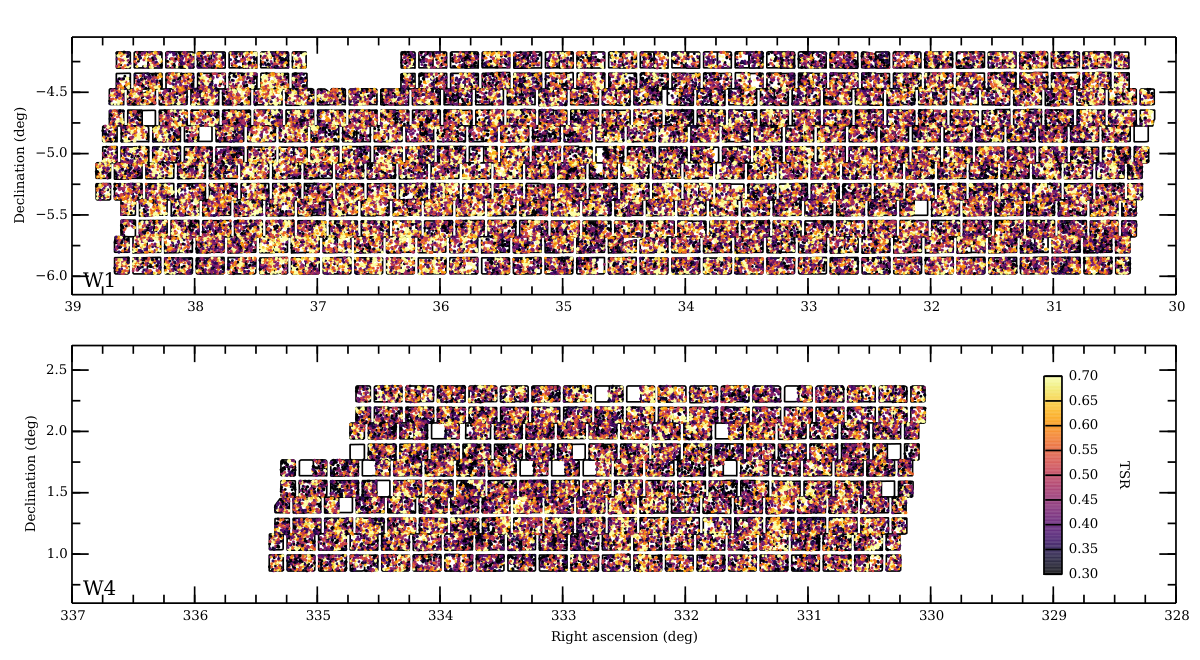
The VIPERS survey covers an overall area of deg2 over the W1 and W4 fields of the Canada-France-Hawaii Telescope Legacy Survey Wide (CFHTLS-Wide). The VIMOS multi-object spectrograph (Le Fèvre et al. 2003) was used to cover these two fields with a mosaic of 288 pointings, 192 in W1 and 96 in W4 (see Fig. 1). Galaxies are selected from the CFHTLS catalogue to a faint limit of , applying an additional vs colour pre-selection that efficiently and robustly removes galaxies at . Coupled with a highly optimised observing strategy (Scodeggio et al. 2009), this doubles the mean galaxy sampling efficiency in the redshift range of interest, compared to a purely magnitude-limited sample, bringing it to 47%.
Spectra are collected at moderate resolution () using the LR Red grism, providing a wavelength coverage of 5500-9500. The typical redshift error for the sample of reliable redshifts is , which corresponds to an error on a galaxy peculiar velocity at any redshift of 163 . These and other details are given in the full PDR-2 release accompanying paper (Scodeggio et al. 2016). A discussion of the data reduction and management infrastructure was presented in Garilli et al. (2014), while a complete description of the survey design and target selection was given in the survey description paper (Guzzo et al. 2014). The dataset used in this paper is an early version of the PDR-2 data, from which it differs by a few hundred redshifts revised during the very last period before the release. In total it includes objects with measured redshifts. As in all statistical analyses of the VIPERS data, only measurements with quality flags 2 to 9 inclusive are used, corresponding to a sample with a redshift confirmation rate of (for a description of the quality flag scheme, see Scodeggio et al. 2016).
In the analysis presented here we shall analyse two redshift sub-samples of the whole survey (W1 + W4) in the ranges and , including respectively 30 764 and 35 734 galaxies.
2.2 Redshift distribution
The redshift distribution of the galaxy sample is shown in Fig. 2. At , it follows the typical decay in the number of objects expected for a magnitude-limited survey, while the rapid fall of the counts at is the result of the colour-colour pre-selection. In de la Torre et al. (2013) it was shown that this histogram can be modelled analytically by the functional form
| (2) |
where , , and are fitting parameters. The term (Colour Sampling Rate) describes the colour-colour pre-selection in terms of an error function transitioning between and around redshift , i.e. where the transition redshift and the transition width are free parameters. As shown in Scodeggio et al. (2016), is unity for , corresponding to a purely magnitude-limited selection.
The best fit of Eq. 2 to the final VIPERS data is shown by the red curve in Fig. 2. Such modelling of the redshift distribution is an important and sensitive ingredient when estimating galaxy clustering, as we discuss in Sect. 3 and in de la Torre et al. (2013). We compare it with the technique (Cole 2011; de la Torre et al. 2013, e.g.) shown in Fig. 2 with the purple curve. Although we find no significant difference in the resulting clustering between the two methods, here we chose to use the method, as in the companion paper of de la Torre et al. (2016). A further method often used in the literature is that of smoothing the observed redshift distribution with a Gaussian kernel (as for instance in the parallel papers by Rota et al. 2016 and Wilson et al. 2017).
2.3 Mock galaxy samples
In order to test the details of the analysis as well as the modelling of RSD, we make use of a suite of mock galaxy catalogues designed to be a realistic match to the VIPERS final dataset. These have been constructed from the Big MultiDark N-body simulation (Klypin et al. 2016), which assumes a flat CDM cosmology with and covers a volume of . The construction of the mock samples is described in de la Torre et al. (2016) and is based on the method detailed in de la Torre et al. (2013). We refer the reader to these papers for details and only give a brief overview of the adopted method in the following.
153 independent lightcones have been extracted from the simulation volume, which follow the geometry of the VIPERS W1+W4 fields. The dark matter haloes identified in the simulation have been populated with galaxies using the halo occupation distribution (HOD) technique. Because of the halo mass resolution of the simulation which is too large to host the faintest galaxies observed in VIPERS, the method of de la Torre & Peacock (2013) has been applied to reconstruct haloes below the resolution limit. Each halo has then been populated with galaxies according to its mass as described by the HOD. The latter has been calibrated directly on the VIPERS data as presented in de la Torre et al. (2013). To obtain fully realistic VIPERS mocks one needs to reproduce the VIPERS survey selection function. This has been done following several steps. First, the magnitude cut and the effect of the colour selection on the radial distribution of the mocks have been applied. The mock catalogues thus obtained are similar to the parent photometric sample used as target galaxy sample for spectroscopy in VIPERS. The slit-positioning algorithm with the same setting as for the data has further been applied to parent mock catalogues. This allows us to reproduce the VIPERS footprint on the sky, the small-scale angular pair incompleteness, and the variation of TSR across the fields. Finally, random redshift errors has been added to mock galaxy redshifts, similar to that present in the data. This procedure allows us to produce realistic mock galaxy catalogues that contain the detailed survey completeness function and observational biases of VIPERS.
3 Galaxy clustering estimation
We quantify galaxy clustering in redshift space by estimating the anisotropic two-point correlation function , where is the redshift-space separation of galaxy pairs and is the cosine of the angle between the separation vector and the line of sight. We generate a catalogue of randomly distributed objects subject to the same angular and radial selection as the true data, and use the Landy & Szalay (1993) estimator:
| (3) |
where , , and are respectively the normalized galaxy-galaxy, galaxy-random, and random-random pair counts in bins of () and (). This estimator has been shown to provide a nearly unbiased estimate of the two-point correlation function, while minimising its variance (Landy & Szalay 1993). We typically use random samples with 30 times more objects than in the true data, to reduce their shot noise contribution to a negligible amount.
In this work we shall estimate the growth rate by fitting RSD models not to the full shape of , but rather to its first two even multipole moments, and , defined as
| (4) |
where is the -th order Legendre polynomials. Such an approach is normally preferred in order to prevent the size of data vectors and the resulting covariance matrix from becoming too large for practical computation (but see Mohammad et al. 2016 for discussion of some drawbacks of this choice).
4 Systematic selection effects
The VIPERS angular selection function is the result of combining several different angular completeness functions. Two of these are binary masks (i.e. describing areas that are fully used or fully lost). The first mask is related to defects in the parent photometric sample (mostly areas masked by bright stars) and the other to the specific footprint of VIMOS and how the different pointings are tailored together to mosaic the VIPERS area. These masks are easily accounted for when defining the area and the auxiliary random samples for clustering measurements.
A more complex selection is related to the incomplete target sampling of VIPERS: on average 47% of the targets satisfying the VIPERS selection criteria can be placed behind a slit and observed, defining what we call the average Target Sampling Rate (TSR). In principle, we should also account for the colour-colour pre-selection of the target sample, which introduces a Colour Sampling Rate (CSR: see Scodeggio et al. 2016). In practice, since the CSR can be safely assumed to be constant over the survey area (thanks to the particularly careful homogenization of the parent sample photometry – see Guzzo et al. 2014), its effect is absorbed into the fit or model describing the smoothed redshift distribution, as in Eq. (2). In any case, the CSR is consistent with being unity for . Finally, we have also to take into account how the probability of measuring the redshift of a targeted galaxy depends on observational conditions or technical issues (which can be location-dependent), which we call the Spectroscopic Success Rate (SSR). The relative relevance, modelling and overall impact of all these effects is described in more detail the following sections.
4.1 Slit collisions


A multi-object spectrograph survey must inevitably face the limitations imposed by the mechanics of how light from the targets is collected on the focal plane. Either fibres or ‘slitlets’ (as in the case of VIMOS) impose a minimum physical size below which the spectrum of two adjacent galaxies on the sky cannot be collected at the same time. This suppresses completely the small-scale clustering amplitude, unless multiple telescope visits of the same field are performed (which is not the case with VIPERS). Furthermore, the same limit on close pairs causes high-density regions on the sky to be more poorly sampled with respect to low-density regions; this introduces a mismatch that, as we shall show, affects the amplitude of clustering on all scales. In VIMOS, this effect is further enhanced by the slit-positioning optimisation software (Bottini et al. 2005, SPOC:), which attempts to maximise the number of slits observed in each quadrant and as such tends to homogenize the angular distribution of targets.
Furthermore, in a multi-slit spectrograph such as VIMOS the dispersed spectrum is imaged directly onto the detector. As is evident from Fig. 3, this creates another ‘forbidden zone’ perpendicular to the slit, where no other target can be observed without causing two spectra to overlap (unlike in fibre spectrographs, where fibres are typically taken away from the telescope to a standing spectrograph and the spectra conveniently aligned and packed on the CCD). Since the projected length of the spectrum on the detector is much larger than the corresponding size of the slit, this introduces another typical scale below which the number of measured angular pairs will be reduced, again limiting the sampling of overdensities on the sky. In VIPERS, the spectral dispersion is always oriented along the North-South direction, so the depletion of galaxy pairs will be anisotropic on the sky and will be larger along the declination direction.
The impact of these effects on angular clustering is quantified in Fig. 4, where in the top panel we have plotted for both the average of 153 mocks (solid lines) and the VIPERS data (filled points) the angular correlation function of the parent and spectroscopic samples ( and , respectively). The bottom panel shows instead the ratio of the corresponding numbers of pairs (bottom panel), defined as
| (5) |
In this figure we find clear evidence of the two angular scales discussed earlier, which are related to the width and length of the spectra; these and identified in the figure by the vertical dashed lines. The origin of this effect can be better identified if we split the separation angle into its components along the right ascension and declination directions, and . The angular completeness map , corresponding to Eq. (5) is shown in Fig. 5. Here the ‘shadow’ of the target spectra is recognisable as the rectangular region with nearly zero counts at small separations. The few residual counts in this area are produced by the small variations in the slit length, together with the effect of the few serendipitous targets observed by chance within the slit of a primary target.
Translated to spatial scales, this angular selection function results in a strong suppression of the clustering amplitude below , as shown by the dotted line in Fig. 6 . In de la Torre et al. (2013), we corrected for this effect by up-weighting each galaxy-galaxy pair at a given angular separation by the inverse of the corresponding value of , i.e.
| (6) |
We shall discuss the effectiveness of this weight together with the correction of the large-scale effect of the TSR, at the end of the next section.
4.2 Larger-scale effects
Along with the drastic suppression at small separations, the physical size of the slits is responsible for the inhomogeneous sampling between high- and low-density regions across a single VIMOS quadrant. This translates in an almost constant suppression of the clustering amplitude on scales above . The correcting scheme we discuss here builds upon the original approach of de la Torre et al. (2013), in which galaxies are assigned a further weight
| (7) |
In that paper, however, the TSR used for each galaxy was simply the average value over the corresponding VIMOS quadrant; in this way, all target galaxies in a quadrant were up-weighted by the same factor. As shown by the dot-dashed curve in Fig. 6, when considering the real-space correlation function this procedure has limited effect (note however than when combined with the small-scale boost, it provides a better correction: see Fig. 8 of de la Torre et al. 2013).
The improved correction adopted here uses instead a local estimate of the TSRi, defined as the ratio of the local surface densities of target and parent galaxies (i.e. before and after applying the target selection); these are estimated as detailed below and then averaged within an aperture of a given shape and size. If we call these quantities and , the TSRi is defined as
| (8) |
The continuous fields are obtained, starting from the discrete distributions of parent and target galaxies, using a Delaunay tessellation (Delaunay 1934) to estimate the density at the position of each galaxy, and then linearly interpolating. These two continuous fields are then used to compute the values of and within an aperture of a given shape and size.
We identified the best-performing geometry for this aperture through the tests shown in Fig. 6. The overall correction is remarkable, since we are able to accurately recover the parent at large separations, both with a circular and a rectangular aperture. The rectangular aperture is the one providing the best correction to real-space clustering, which can be understood in terms of the anisotropy of the spectral ‘shadows’ discussed earlier. The optimal size of the rectangular aperture is found to be . The resulting distribution of the TSRi values over the survey regions is shown in Fig. 1.
4.3 Redshift dependence of angular corrections
Some of the corrections for angular selection biases do have an effect also on the redshift distribution. Fig. 7 shows the effect of correcting for the TSR and SSR on the observed redshift distribution of the VIPERS data. While the TSR does not introduce a significant redshift dependence, the application of the SSR boosts the expected number of galaxies in the distant () part of the sample. This clearly reflects the increased inefficiency to measure redshifts for more and more distant objects. To be fully consistent with the data, then, the random samples used for the clustering analyses will have to be weighted accordingly.
5 Two-point correlations from the VIPERS data

We thus proceed to estimate the redshift space correlation function and its moments for the VIPERS survey, adopting the weighting scheme discussed in the previous sections, which we recap for convenience:
- •
- •
Pair counts in the two-point correlation function estimator of Eq. 3 are then expressed as
| (9) | ||||
| (10) | ||||
| (11) |
where is equal to unity for in and in , and null otherwise.
The final performance of this weighting scheme on the recovered monopole and quadrupole of the redshift space correlation function are shown in Fig. 8, for the two redshift ranges considered in the analysis. The combined correction recovers the amplitude of the monopole at the level, down to the scale, yielding a quasi-unbiased estimate of on all comoving scales that will be used for the RSD fitting. As for the quadrupole, we are able to have a reliable measurement of ( deviation from the fiducial value) down to a few . This is an encouraging result: any uncorrected anisotropy from selection effects would be in danger of inducing a spurious contribution to the quadrupole, since this is our main measure of anisotropy.
Fig. 9 shows the measurement of the anisotropic correlation function obtained from the full VIPERS data at and . A bin size Mpc has been used in both and directions. We combine the results coming from the two VIPERS fields W1 and W4 simply by summing up the pair counts in each bin of separation and normalising for the total number of objects.
6 Covariance matrix and error estimation
Given the intrinsic correlation among different bins of the two-point correlation function (and consequently of its multipoles), it is essential to obtain a reliable estimate of the covariance matrix to be used during the fitting procedure. The fit is carried out performing a maximum likelihood analysis of the data given the RSD model, that can be more easily described as the search throughout the parameter space of the position minimising the likelihood function defined as
| (12) |
Here the observable is the monopole-quadrupole combined vector; is the precision matrix (the inverse of the covariance matrix); is the total number of data points; and indices and stand respectively for data and model.
The covariance matrix is organised in four blocks corresponding to the monopole-monopole, quadrupole-quadrupole and monopole-quadrupole cross covariance (two identical blocks in the latter case). The full monopole-quadrupole covariance matrix is estimated from the 153 mock realisations as
| (13) |
where is the number of independent realisations used to estimate the covariance, is the monopole-quadrupole vector, indices run over the data points and index runs over different realisations. The mean value is estimated by averaging the measured values from different realisations, namely
| (14) |
The corresponding correlation matrices obtained in this way for the two redshift sub-samples are shown in Fig. 10.
Given the large number of mock samples, the estimate and the inversion of the covariance matrices can be achieved with good accuracy. However, the use of a finite number of mocks has two implications. Firstly, the estimated precision matrix obtained by taking the inverse of is biased with respect to the true one, , with the difference being well-represented by an inverse Wishart distribution. Furthermore, the precision matrix contains statistical errors that propagate to the parameter space, affecting the derived errors on the cosmological parameters. We follow Percival et al. (2014) and correct for these effects by applying two correction factors. In the first case, we can remove the systematic bias of the precision matrix by rescaling as
| (15) |
The latter correction factor involves the total number of data points and realisations . It takes into account the typical skewness characterising an inverse Wishart distribution and is capable of providing an unbiased estimate of the precision matrix (Hartlap et al. 2007). In the second case, the propagation of errors from the precision matrix to the derived parameters can be corrected by defining
| (16) |
and applying the correction factor
| (17) |
to the estimated parameter covariance. In the previous equation, is the total number of free parameters.

7 Modelling redshift-space distortions
Redshift-space distortions arise because the apparent position of galaxies is modified by the Doppler effect of their peculiar velocity . In this way, the redshift-space position of galaxies located at becomes
| (18) |
where is the scale factor, is the expansion rate and is the component of the galaxy peculiar velocity along the line of sight. Invoking mass conservation, the redshift-space density field can be expressed as a function of its real-space counterpart as
| (19) |
The targeting of high-redshift galaxies in VIPERS means that the largest pair separations are much smaller than the distance from the observer, so we can use the small-angle plane-parallel approximation; the Jacobian of the real-to-redshift space transformation then reduces to
| (20) |
where the normalized velocity field is defined as . Substituting this expression inside Equation (19) it follows that
| (21) |
Taking the Fourier transform of this equation and making explicit the dependence on , we obtain
| (22) | |||||
In the hypothesis of a perfectly irrotational velocity field (an assumption which is fair as long as we consider large-scale fluctuations), we can define the divergence of the velocity field as . Therefore, Equation (19) can be written as
| (23) |
where denotes the Laplace operator. In Fourier space it can be proved that the operator featuring the previous equation can be simplified as , where is the cosinus of the angle between the wave vector and the line of sight. Taking the Fourier transform of Eq. (23) and substituting the Laplace operator with the previous expression, it follows that
| (24) |
The redshift-space power spectrum can thus be written as (Scoccimarro et al. 1999)
| (25) | |||||
with and . This last equation completely describes the anisotropies produced by peculiar velocities on the clustering of matter particles at each separation. Here, the only assumption is the plane-parallel approximation limit.
It is possible to identify two main regimes within which distortions manifest themselves. At large separations, matter has a coherent flow towards overdense regions. In this regime, the velocity field is mainly irrotational (Bernardeau et al. 2002) and can thus be described by its divergence . These motions produce a systematic distortion of the large-scale distribution along the line of sight. This ‘Kaiser effect’ (Kaiser 1987) is basically produced by the terms inside the square brackets in Eq. (25).
In contrast, within the typical scale of haloes, galaxy orbits cross each other: there is a random dispersion in velocities at a given point, which convolves the redshift-space structure in the radial direction. The clustering amplitude is thus suppressed on small scales, and structures appear stretched along the line of sight in the so called ‘Fingers of God’ (Jackson 1972). This effect is mainly generated by the exponential pre-factor involving the moment generating function of the velocity field.
Eq. (25) is hard to use in its given form, because we lack an analytic formula for the ensemble average term inside the integral, particularly in the strongly non-linear regime. But a number of simpler approximate forms have been suggested, which aim to provide a satisfactory representation of the redshift-space power spectrum measured from galaxy surveys:
– Kaiser model (Kaiser 1987): within the linear theory approximation, the exponential pre-factor can be suppressed since its impact on the largest scales is negligible and . If the galaxy-matter bias relation is also assumed to be linear (), it follows that
| (26) |
where is the linear real-space matter power spectrum and is the linear galaxy bias.
– Dispersion model (Peacock & Dodds 1994): although the previous model can reproduce the apparent enhancement of clustering at large separations, it fails in the description of the non-linear regime. The latter can be treated in a phenomenological way, by artificially suppressing the linear theory predictions to account for the effect of the Fingers of God. Eq. (26) can thus be written as
| (27) |
where is an analytical damping factor. This term depends on a nuisance parameter , which plays the role of a pairwise velocity dispersion. The basic assumption of the dispersion model is that is not scale-dependent, but rather can be fitted as a free parameter. An useful extension of this model is to replace the linear by a non-linear version (using an analytic approximation such as HALOFIT). This then allows the dispersion model to give the correct prediction for : such modes run transverse to the line of sight and undergo no RSD effect. Note that some of the alternatives discussed here fail to match the real-space power exactly at : this is because they are attempting the harder task of predicting the non-linearities, rather than taking them from a fit to -body simulation data.
– Scoccimarro model (Scoccimarro 2004): as soon as the mildly non-linear regime is entered, the density and velocity divergence fields must be treated separately to account for the non-linear mode coupling between them. The ansatz proposed by Scoccimarro is that the exponential pre-factor inside Eq. (25) can be decoupled from the Kaiser term, so that its impact on the clustering is limited only to the smallest scales. In this case, it can be replaced with a damping factor similar to the one already used in the dispersion model, leading to
| (28) |
where and are respectively the density-velocity divergence cross-spectrum and the velocity divergence auto-spectrum. When applying this (and the following) model to real data, these quantities cannot be obtained from the data under analysis. As such, applications of this (and the following) model have used empirical fitting functions calibrated using numerical simulations (Jennings et al. 2011). In a parallel paper (Bel et al. 2017), new, more general formulas are proposed:
| (29) |
| (30) |
where is the linear matter power spectrum and is a parameter representing the typical damping scale of the velocity power spectra. This can be well described as
| (31) |
where are the only free parameters of the fit. These forms for and have valuable, physically motivated properties: they naturally converge to in the linear regime, including a dependence on redshift through .
Full details on the derivation and performances of these fitting formulas are presented in Bel et al. (2017). Their use in the analysis presented in the following sections is a significant improvement over previous applications of the Scoccimarro and TNS (Taruya et al. 2010) models, as it allows us to extend our tests to smaller scales and apply the models to high redshifts as sampled by VIPERS.
– Taruya (or TNS) model (Taruya et al. 2010): the non-linear mode coupling between the density and velocity divergence fields is responsible for a systematic bias between measurements of the power spectrum and its prediction using the previous RSD model. The origin of this deviation is the additional terms inside Eq. (28), which are not accounted for within the previous ansatz. The corrected model can be written as
| (32) |
where and are terms derived using perturbation theory, which aim to account for the density and velocity divergence couplings with the exponential pre-factor in Eq. (25). See de la Torre & Guzzo (2012) for the details of its application to biased tracers.
All the tested RSD models feature a phenomenological damping factor . The function damps the power spectra in the Kaiser term but also partially mimics the effects of the pairwise velocity distribution in virialised systems. The expected analytic form of the damping factor on large enough scales assuming the Scoccimarro ansatz is Gaussian (Scoccimarro 2004); but analyses of simulated galaxy samples (de la Torre & Guzzo 2012) have shown that a Lorentzian template provides a better practical fit.
Models in equations 27, 28 and 32 are all tested in the next sections to understand their impact on the recovery of the growth rate. In all cases, at each step of our Monte Carlo Markov chains we generate the full anisotropic redshift-space power spectrum. For this we make use of CAMB with the latest HALOFIT prescription for the non-linear (Takahashi et al. 2012), and Eqs. 29 and 30 to generate the and power spectra. The normalisation of the latter real-space power spectra, which can be set by , is degenerate with and . This is why one generally parametrises RSD models in terms and parameters. In the case of the TNS model, however, this is not possible directly since the term involves sub-terms that are not multiples of the or parameters (Taruya et al. 2010; de la Torre & Guzzo 2012, e.g.). Therefore for the TNS model, and for the others for consistency, we decide to treat , , , as free distinct parameters in the fit, and provide derived constraints on a posteriori from the MCMC chains.
It is important to emphasize that not only plays a role in shaping the term, it also controls the level of non-linearity in , , and . In particular for , the HALOFIT non-linear correction to the linear matter power spectrum is computed at each step of the MCMC according to the tested value of . This represents a significant improvement over what is usually done in RSD analyses, where is fixed to its fiducial value for the description of .
In the end, we measure the Fourier-space multipole moments as
| (33) |
and convert them to their configuration space counterparts as
| (34) |
where denotes the spherical Bessel functions.
8 Tests of RSD models
We test in this section the RSD models introduced previously on our set of mock catalogues. In practice, analysing each mock and averaging the measurements would be computationally infeasible, considering the large number of configurations to be tested. We thus chose to average the monopole and quadrupole measurements over the mocks, scale the covariance matrix properly, and fit the models to these average measurements. The aim is to reach a statistical uncertainty that is a factor smaller than a single VIPERS survey, to be able to detect potential systematics as small as . This process is more revealing and can show how well a given model performs in recovering the detailed shapes of the quadrupole and monopole correlation function.
We perform likelihood analyses of the mock mean measurements in different configurations, starting the ideal case and moving on to that in fully realistic conditions. All likelihood analyses are carried out using an MCMC code, whose output has been cross-checked with the independent MCMC code used in de la Torre et al. (2016). We select flat priors for the full set of free parameters, using boundaries that allow a large set of late-time evolution cosmological models to be considered as possible alternatives to standard CDM. The full list of priors is shown in Table 1, while the best-fit values for the parameters are listed in Table 2. We vary the minimum scale of the fit to understand how to select the best fitting range for the VIPERS data – we expect all RSD models to fail at sufficiently small and non-linear scales. The maximum scale of the fit is fixed at , above which errors on the VIPERS measured monopole and quadrupole become too large.
8.1 Ideal case
We first study the ideal case that neglects the complex VIPERS angular selection by using the parent mocks. Here we consider mock measurements from the full redshift range probed by VIPERS, i.e. , to avoid tuning the procedure towards small systematic deviations on the two redshift bins. The relative difference of the recovered with respect to the fiducial one is shown in Fig. 11. Redshift errors are not considered here to understand how different RSD models behave in the absence of any observational bias. Two types of small-scale damping factor are tested: the Lorentzian (filled symbols) and Gaussian (dashed lines) forms. The overall trend of models using Lorentzian damping favours the TNS model: it yields almost unbiased measurements of the growth rate down to . Some overestimation is however seen for minimum scales close to , which in fact corresponds to the zero-crossing scale of the quadrupole .
In contrast, both dispersion and Scoccimarro models consistently underestimate the growth rate with an error that fluctuates between 5–10%. Evidently, in all the cases the choice of a Lorentzian damping yields smaller systematic deviations than with a Gaussian damping. This is reflected by the trend of the dashed lines, which are close to the corresponding markers only when the minimum fitting separation is larger than , while rapidly deteriorating when smaller separations are included in the fit. This is highlighted in Fig. 12, where the different best-fitting models for the monopole and quadrupole using are directly compared to the mock data. Using a Gaussian damping, the model is no longer able to provide a good description of and . Actually, the fit is mostly dominated by the small scales, whose data points have the smallest errors, and this explains why separations above are apparently the ones giving the strongest deviation between model and data. This result is in close agreement with previous work on the subject (Bianchi et al. 2012; de la Torre & Guzzo 2012, e.g.).
8.2 Case with redshift errors
So far no redshift error was assumed in the mock samples. However, real VIPERS redshifts have a significant uncertainty, which clearly impact observed redshift-space distortions. We know from the multiple redshift measurements (Scodeggio et al. 2016) that the redshift error probability distribution for the VIPERS sample of reliable redshifts used here, is well described by a Gaussian with standard deviation . This corresponds to a dispersion in galaxy peculiar velocity of 163 km s-1.
By applying random errors to mock galaxy redshifts following the VIPERS observed distribution, we can effectively see additional distortions. These are shown in Fig. 13, where one can see how the shapes of the monopole and the quadrupole are affected. The imprint of redshift errors is similar to that of a small-scale damping of the power spectrum. While the monopole is damped below , the quadrupole is corrupted over a range extending out to . Clearly, this effect needs to be carefully handled or modelled, if one hopes to recover an unbiased value for the growth rate. The consequences of not correcting for this effect are shown by the dashed lines in Fig. 14, where we are repeating the tests of Fig. 11, but now including redshift errors. As feared, there is a significant deviation from the values of previously measured with the models in the best configuration, i.e. with the Lorentzian damping.
Rather than correcting for redshift errors in the measurements, as performed for the angular selection selection, it is better to include it in the modelling. It is intuitive to supplement the models with a convolution by an extra Gaussian distribution with standard deviation fixed to the VIPERS rms value of , which corresponds to
| (35) |
in terms of line-of-sight comoving separation. The filled symbols in Fig. 14 show how with this extra damping term we recover a performance similar to the more idealised case of Fig. 11.
We therefore adopt the TNS model with Lorentzian damping and Gaussian error damping, as our reference model for the final RSD analysis of the VIPERS data. However, we will also test for consistency the behaviour of the other two models on the actual data, to verify whether the trends seen in the mocks are confirmed.
8.3 Fully realistic case
We now turn to the case including fully realistic observing conditions. This means considering the target selection (masks, TSR, SSR, etc.) and limiting the samples to the same redshift ranges covered by the data and including redshift errors. The results that we obtain are shown in Fig. 15. The trends of the systematic error as a function of are less stable than in the previous case, although the general behaviour and relative performances of the models are the same. The variations gives us an idea of the impact of the selection function on samples this size. Again, we see some instability in the TNS model (at least in the bin ) when the minimum scale of the fit is chosen around . When we look into the MCMC results in more detail, we see that in this case the Markov chain tends to drift towards unrealistic values of , which are outside of the prior range defined in Table 2. This seems to be related to the difficulty of TNS model to reach a stable fit in the region where the quadrupole crosses zero. As soon as we include smaller scales (or we move away to larger ones), the regular trend is recovered. Nevertheless, we confirm the TNS model as the best performing one, with systematics down to the smallest probed minimum scales.
Overall, the different tests performed on the mock catalogues indicate that we can safely use the TNS model with the appropriate damping functions as well as a minimum fitting scale of . This is the configuration that we adopt for the analysis of the data.
9 VIPERS RSD results
| Parameters | Uniform prior |
|---|---|
| Parameters | ||
|---|---|---|
We present in this section the results of the RSD analysis of the VIPERS final dataset. We apply the methodology described in the previous sections to the VIPERS galaxy sample. In the likelihood analysis we impose rather broad uniform priors on the sampling parameters. These are reported in Table 1. Since and are treated as separate parameters in the modelling, despite their intrinsic degeneracy, we need to impose sensible priors on them. In fact the most sensitive prior is that on , as it is the main parameter entering the non-linear modelling of RSD. To define a sensible and realistic prior, while allowing room for deviations from GR, we base our choice on the Effective Field Theory of dark energy formalism (Gubitosi et al. 2013; Bloomfield et al. 2013; Gleyzes et al. 2013), which allows a description of various kinds of dark energy models and modifications of gravity to be expressed in a self-consistent framework that includes the growth rate of structure (Piazza et al. 2014; Perenon et al. 2015). The latter work shows that the range spanned by for stable theories can vary significantly, suggesting a range [, ] as appropriate to account for early- and late-time dark energy models at the redshifts covered by VIPERS (for definitions, see Perenon et al. 2016). This excludes some more extreme modified gravity models, but avoids non-physical degeneracies that arise in the likelihood for some particular values of outside of this range. This choice is corroborated by our parallel complementary analysis using the same data by de la Torre et al. (2016), in which the combination of RSD with galaxy-galaxy lensing constrains directly , allowing a broader prior at the outset.
The measurements that we finally obtain using our standard configuraton and previously discussed parameter priors are and . We consider these as our reference measurements in this work and discuss their cosmological implications in the next section. The measurements and best-fitting model monopole and quadrupole correlation functions obtained in the two considered redshift bins are shown in Fig. 16. The corresponding best-fit values for the derived parameters are reported in Table 2.
It is interesting to verify a posteriori whether the trends and relative RSD model performances as a function of established from the mock catalogues are similar to those seen in the real data. It is of course clear that any trend will be less significant, as the data are statistically equivalent to considering just one of the 153 mock catalogues. In the left panel of Fig. 17, we show the result of this exercise, where the measured values of as a function of are shown for the different tested models. To ease comparison, we have reported in the right panel and using the same scale, the corresponding results from the mock test for the realistic case (i.e. those of Fig. 15). Apart from the different statistical errors, it is surprising to note how the three tested RSD models provide virtually identical results in the real data, as opposed to the behaviour seen in the mock catalogues. Moreover, it seems that in the data the variation of the measurements with minimum scale are not driven by the adequacy of the model down to those scales, but rather by statistical uncertainties in the measured galaxy correlation functions. The similarity in the results obtained from the different models is confirmed directly by the values of the reduced , which turn out to be very similar. By directly looking at the posterior likelihood distributions of the parameters obtained with the three models in Fig. 18 (for the high-redshift bin), we can see that each model provides slightly different parameters degeneracies, although after marginalization, posterior likelihood distributions are almost identical for the three RSD models, with only a slightly larger statistical uncertainty with the TNS model. However, some trends seen in the mock results are recognised in the data, as for example the preference of the TNS model in the high-redshift sample to deliver larger values of when is close to the zero-crossing scale of the quadrupole.
Finally, it is important to emphasize the global non-linear approach to RSD that has been used in this analysis. We have used rather small non-linear scales in the fit, and by adopting a consistent modelling for the non-linearities in the real-space density and velocity divergence power spectra, we can obtain further cosmological insight. The level of non-linearity in our analysis is controlled by one single parameter, , and we find that by letting this parameter vary, we can partly break the standard degeneracy that dominates on linear scales between , , and parameters. If we marginalise the posterior likelihood function over the , , parameters, we obtain the following direct growth rate and constraints: and . A similar approach has been adopted in de la Torre et al. (2016), where this is strengthened by additional constraints from galaxy-galaxy lensing. In particular, the latter allows improving constraints while keeping similar uncertainties on . A detailed discussion of these results is given in de la Torre et al. (2016). Overall, these findings demonstrate the additional constraining power encapsulated in quasi-linear scales, which can be used to break degeneracies and further improve the precision of measurement of the growth rate of structure.
10 Discussion and conclusions
The measurements of the growth rate of structure times that we obtained are
| (36) | |||||
| (37) |
These values are confronted in Fig. 19 with different measurements, including results from other surveys, the VIPERS earlier PDR-1 dataset, and parallel works analysing with complementary techniques analogous subsets of the VIPERS PDR-2 dataset. It may look surprising that there is no appreciable improvement in the error bars between the former measurement from the PDR-1 (de la Torre et al. 2013, red circle) and the new PDR-2 estimate in a comparable redshift bin, despite a increase in the sample size. As discussed in de la Torre & Guzzo (2012), this is essentially a price to pay for the more sophisticated treatment of nonlinear effects through the TNS model, which increases the degrees of freedom.
The parallel PDR-2 results include measurements obtained from the combination of RSD with galaxy-galaxy lensing (de la Torre et al. 2016) or using the void-galaxy cross-correlation (Hawken et al. 2016). In forthcoming papers, we shall additionally present further pieces of this combined approach, using specific colour-selected subsamples (Mohammad et al. 2017) or the linearised density field in Fourier space (Wilson et al. 2017), to minimise the need for non-linear corrections. All these papers represent complementary approaches towards understanding the current limitations we face in our ability to extract in practice the value of these parameters from the modelling of RSD.
The values measured by these different techniques on the same VIPERS data as well as from other surveys at similar redshifts are virtually all compatible within 1- and agree with the predictions of a CDM model governed by Einstein gravity. But on a larger sample, with much smaller statistical errors, greater care would be needed to test for possible systematic biases that might still be hidden in one or more of the analyses. The application of such a variety of approaches to VIPERS has been made possible by the specific properties of the survey, in particular its dense sampling and rich content of information. With a sparse sampled survey, which is the approach of most of the cosmologically-oriented surveys, it would have been impossible to characterise accurately the density field and apply the clipping linearisation technique of Wilson et al. (2017), or reliably detect cosmic voids such as those used in Hawken et al. (2016). At the same time, a survey with limited imaging information would not permit investigation of the selection of optimal sub-populations (or the combination of different ones), as we are pursuing in Mohammad et al. (2017), or exploit the combination of RSD with lensing, as we have done in de la Torre et al. (2016) and which should be exploited to the fullest by Euclid mission (Laureijs et al. 2011) in the next decade. We therefore believe that the detailed investigation of the properties of RSD within VIPERS should serve as a valuable foundation for next-generation studies of greater statistical power.
Acknowledgements.
We acknowledge the crucial contribution of the ESO staff for the management of service observations. In particular, we are deeply grateful to M. Hilker for his constant help and support of this program. Italian participation to VIPERS has been funded by INAF through PRIN 2008, 2010, 2014 and 2015 programs. LG and BRG acknowledge support from the European Research Council through grant n. 291521. OLF acknowledges support from the European Research Council through grant n. 268107. JAP acknowledges support of the European Research Council through the COSFORM ERC Advanced Research Grant (# 670193). GDL acknowledges financial support from the European Research Council through grant n. 202781. RT acknowledges financial support from the European Research Council through grant n. 202686. AP, KM, and JK have been supported by the National Science Centre (grants UMO-2012/07/B/ST9/04425 and UMO-2013/09/D/ST9/04030). EB, FM and LM acknowledge the support from grants ASI-INAF I/023/12/0 and PRIN MIUR 2010-2011. LM also acknowledges financial support from PRIN INAF 2012. SDLT and MP acknowledge the support of the OCEVU Labex (ANR-11-LABX-0060) and the A*MIDEX project (ANR-11-IDEX-0001-02) funded by the "Investissements d’Avenir" French government program managed by the ANR. Research conducted within the scope of the HECOLS International Associated Laboratory, supported in part by the Polish NCN grant DEC-2013/08/M/ST9/00664. TM and SA acknowledge financial support from the ANR Spin(e) through the French grant ANR-13-BS05-0005.References
- Anderson et al. (2012) Anderson, L., Aubourg, E., Bailey, S., et al. 2012, MNRAS, 427, 3435
- Bel et al. (2017) Bel, J. et al. 2017, in preparation
- Bernardeau et al. (2002) Bernardeau, F., Colombi, S., Gaztañaga, E., & Scoccimarro, R. 2002, Phys. Rep, 367, 1
- Beutler et al. (2011) Beutler, F., Blake, C., Colless, M., et al. 2011, MNRAS, 416, 3017
- Beutler et al. (2012) Beutler, F., Blake, C., Colless, M., et al. 2012, MNRAS, 423, 3430
- Beutler et al. (2016) Beutler, F., Seo, H.-J., Saito, S., et al. 2016, ArXiv e-prints
- Bianchi et al. (2015) Bianchi, D., Gil-Marín, H., Ruggeri, R., & Percival, W. J. 2015, MNRAS, 453, L11
- Bianchi et al. (2012) Bianchi, D., Guzzo, L., Branchini, E., et al. 2012, ArXiv e-prints
- Blake et al. (2011) Blake, C., Brough, S., Colless, M., et al. 2011, MNRAS, 415, 2876
- Bloomfield et al. (2013) Bloomfield, J. K., Flanagan, É. É., Park, M., & Watson, S. 2013, JCAP, 1308, 010
- Bottini et al. (2005) Bottini, D., Garilli, B., Maccagni, D., et al. 2005, PASP, 117, 996
- Cabré & Gaztañaga (2009) Cabré, A. & Gaztañaga, E. 2009, MNRAS, 393, 1183
- Carroll et al. (2004) Carroll, S. M., Duvvuri, V., Trodden, M., & Turner, M. S. 2004, Phys. Rev. D, 70, 043528
- Clifton (2011) Clifton, T. 2011, Progress in Particle and Nuclear Physics, 66, 181
- Cole (2011) Cole, S. 2011, MNRAS, 416, 739
- Colless et al. (2001) Colless, M., Dalton, G., Maddox, S., et al. 2001, MNRAS, 328, 1039
- Contreras et al. (2013) Contreras, C., Blake, C., Poole, G. B., et al. 2013, MNRAS, 430, 924
- de la Torre & Guzzo (2012) de la Torre, S. & Guzzo, L. 2012, MNRAS, 427, 327
- de la Torre et al. (2013) de la Torre, S., Guzzo, L., Peacock, J. A., et al. 2013, A&A, 557, A54
- de la Torre & Peacock (2013) de la Torre, S. & Peacock, J. A. 2013, MNRAS, 435, 743
- de la Torre et al. (2016) de la Torre, S. et al. 2016, A&A submitted
- Delaunay (1934) Delaunay, B. 1934, Bulletin de l’Academie des Sciences de l’URSS, Classe des sciences mathematiques et naturelles, 6, 793
- Dvali et al. (2000) Dvali, G., Gabadadze, G., & Porrati, M. 2000, Physics Letters B, 485, 208
- Fisher (1995) Fisher, K. B. 1995, ApJ, 448, 494
- Garilli et al. (2014) Garilli, B., Guzzo, L., Scodeggio, M., et al. 2014, A&A, 562, A23
- Gleyzes et al. (2013) Gleyzes, J., Langlois, D., Piazza, F., & Vernizzi, F. 2013, JCAP, 1308, 025
- Grieb et al. (2016) Grieb, J. N., Sánchez, A. G., Salazar-Albornoz, S., et al. 2016, ArXiv e-prints
- Gubitosi et al. (2013) Gubitosi, G., Piazza, F., & Vernizzi, F. 2013, JCAP, 1302, 032, [JCAP1302,032(2013)]
- Guzzo et al. (2008) Guzzo, L., Pierleoni, M., Meneux, B., et al. 2008, Nature, 451, 541
- Guzzo et al. (2014) Guzzo, L., Scodeggio, M., Garilli, B., et al. 2014, A&A, 566, A108
- Hartlap et al. (2007) Hartlap, J., Simon, P., & Schneider, P. 2007, A&A, 464, 399
- Hawken et al. (2016) Hawken, A. J., Granett, B. R., Iovino, A., et al. 2016, ArXiv e-print 1611.07046
- Hawkins et al. (2003) Hawkins, E., Maddox, S., Cole, S., et al. 2003, MNRAS, 346, 78
- Hinshaw et al. (2012) Hinshaw, G., Larson, D., Komatsu, E., et al. 2012, ApJS accepted, ArXiv e-print 1212.5226
- Jackson (1972) Jackson, J. C. 1972, MNRAS, 156, 1P
- Jain & Khoury (2010) Jain, B. & Khoury, J. 2010, Annals of Physics, 325, 1479
- Jennings et al. (2011) Jennings, E., Baugh, C. M., & Pascoli, S. 2011, MNRAS, 410, 2081
- Kaiser (1987) Kaiser, N. 1987, MNRAS, 227, 1
- Klypin et al. (2016) Klypin, A., Yepes, G., Gottlöber, S., Prada, F., & Heß, S. 2016, MNRAS, 457, 4340
- Lahav et al. (1991) Lahav, O., Lilje, P. B., Primack, J. R., & Rees, M. J. 1991, MNRAS, 251, 128
- Landy & Szalay (1993) Landy, S. D. & Szalay, A. S. 1993, ApJ, 412, 64
- Laureijs et al. (2011) Laureijs, R., Amiaux, J., Arduini, S., et al. 2011, ArXiv e-print 1110.3193
- Le Fèvre et al. (2003) Le Fèvre, O., Saisse, M., Mancini, D., et al. 2003, in Proc. SPIE, ed. M. Iye & A. F. M. Moorwood, Vol. 4841, 1670–1681
- Linder & Cahn (2007) Linder, E. V. & Cahn, R. N. 2007, Astroparticle Physics, 28, 481
- Mohammad et al. (2017) Mohammad, F. et al. 2017, in preparation
- Mohammad et al. (2016) Mohammad, F. G., de la Torre, S., Bianchi, D., Guzzo, L., & Peacock, J. A. 2016, MNRAS, 458, 1948
- Okumura et al. (2016) Okumura, T., Hikage, C., Totani, T., et al. 2016, PASJ, 68, 38
- Okumura & Jing (2011) Okumura, T. & Jing, Y. P. 2011, ApJ, 726, 5
- Peacock et al. (2001) Peacock, J. A., Cole, S., Norberg, P., et al. 2001, Nature, 410, 169
- Peacock & Dodds (1994) Peacock, J. A. & Dodds, S. J. 1994, MNRAS, 267, 1020
- Peebles (1980) Peebles, P. J. E. 1980, The large-scale structure of the universe (Princeton University Press, 1980. 435 p.)
- Percival et al. (2014) Percival, W. J., Ross, A. J., Sánchez, A. G., et al. 2014, MNRAS, 439, 2531
- Perenon et al. (2016) Perenon, L., Marinoni, C., & Piazza, F. 2016
- Perenon et al. (2015) Perenon, L., Piazza, F., Marinoni, C., & Hui, L. 2015, JCAP, 1511, 029
- Perlmutter et al. (1999) Perlmutter, S., Aldering, G., Goldhaber, G., et al. 1999, ApJ, 517, 565
- Piazza et al. (2014) Piazza, F., Steigerwald, H., & Marinoni, C. 2014, JCAP, 1405, 043
- Planck Collaboration et al. (2015) Planck Collaboration, Ade, P. A. R., Aghanim, N., et al. 2015, ArXiv e-print: 1502.01589
- Reid et al. (2012) Reid, B. A., Samushia, L., White, M., et al. 2012, MNRAS, 426, 2719
- Reid et al. (2014) Reid, B. A., Seo, H.-J., Leauthaud, A., Tinker, J. L., & White, M. 2014, MNRAS, 444, 476
- Riess et al. (1998) Riess, A. G., Filippenko, A. V., Challis, P., et al. 1998, AJ, 116, 1009
- Ross et al. (2007) Ross, N. P., da Ângela, J., Shanks, T., et al. 2007, MNRAS, 381, 573
- Rota et al. (2016) Rota, S., Granett, B. R., Bel, J., et al. 2016, ArXiv e-print 1611.07044
- Samushia et al. (2012) Samushia, L., Percival, W. J., & Raccanelli, A. 2012, MNRAS, 420, 2102
- Sanchez et al. (2016) Sanchez, A. G., Scoccimarro, R., Crocce, M., et al. 2016, ArXiv e-prints
- Satpathy et al. (2016) Satpathy, S., Alam, S., Ho, S., et al. 2016, ArXiv e-prints
- Scoccimarro (2004) Scoccimarro, R. 2004, Phys. Rev. D, 70, 083007
- Scoccimarro et al. (1999) Scoccimarro, R., Couchman, H. M. P., & Frieman, J. A. 1999, ApJ, 517, 531
- Scodeggio et al. (2009) Scodeggio, M., Franzetti, P., Garilli, B., Le Fèvre, O., & Guzzo, L. 2009, The Messenger, 135, 13
- Scodeggio et al. (2016) Scodeggio, M., Guzzo, L., Garilli, B., et al. 2016, ArXiv e-print 1611.07048
- Takahashi et al. (2012) Takahashi, R., Sato, M., Nishimichi, T., Taruya, A., & Oguri, M. 2012, ApJ, 761, 152
- Taruya et al. (2010) Taruya, A., Nishimichi, T., & Saito, S. 2010, Phys. Rev. D, 82, 063522
- Uhlemann et al. (2015) Uhlemann, C., Kopp, M., & Haugg, T. 2015, Phys. Rev. D, 92, 063004
- Weinberg et al. (2013) Weinberg, D., Bard, D., Dawson, K., et al. 2013, ArXiv e-prints
- Weinberg (1989) Weinberg, S. 1989, Reviews of Modern Physics, 61, 1
- Wilson et al. (2017) Wilson, M. et al. 2017, in preparation