Partition-free approach to open quantum systems in harmonic environments: an exact stochastic Liouville equation
Abstract
We present a partition-free approach to the evolution of density matrices for open quantum systems coupled to a harmonic environment. The influence functional formalism combined with a two-time Hubbard-Stratonovich transformation allows us to derive a set of exact differential equations for the reduced density matrix of an open system, termed the Extended Stochastic Liouville-von Neumann equation. Our approach generalises previous work based on Caldeira-Leggett models and a partitioned initial density matrix. This provides a simple, yet exact, closed-form description for the evolution of open systems from equilibriated initial conditions. The applicability of this model and the potential for numerical implementations are also discussed.
I Introduction
Much of the work in the canon of physics has been derived under an assumption of isolation, where the system of interest has no interaction with its environment. Often, particularly in the classical regime, this approximation has been successful in generating accurate predictions. There are however numerous systems whose behaviour cannot be explained by their actions in a vacuum [1]. In these cases stochastic terms are used, often as an a priori part of the model (and without proper justification), to capture the effect of the environment. Brownian motion is the most famous case of this technique in classical physics, but quantum physics and its applications have many examples where a similarly careful treatment of external effects is required [2, 3, 4]. These systems can collectively be termed open dissipative quantum systems, and the problem of how to most accurately model them remains an active field of research.
Approaches to these systems can be split into two broad categories. The first method uses the paradigmatic example of a damped system, where the damping is an effective loss-mechanism that approximates the environment’s effect and fluctuations are neglected. A typical example of this is the early work of Kerner and Stevens on sets of damped harmonic oscillators [5, 6]. The basis of this method in classical, phenomological equations means that it is capable of providing exact solutions for some simple systems, such as the damped harmonic oscillator. These solutions are however undermined by being fundamentally incompatible with quantum mechanics. This can be illustrated by the fact that there are no time-independent Hamiltonians that can replicate the equation of motion for a damped oscillator,
| (1) |
which has frequency and friction . While there exists a time-dependent Hamiltonian that leads to this equation of motion [7], after quantisation the fundamental commutation relation becomes time-dependent [8]. This unphysical result means that another approach to dissipative systems, to be detailed below, is the method of choice.
In this approach, pioneered by Callen, Welton, Senitzky and Lax, dissipative systems are modelled as a primary system (the “open system”) of interest coupled to an explicit secondary system (the “environment” or “heat bath”) which together describe the overall system being modeled (the “total system”) [9, 10, 8]. In comparison to the first method, this model is lossless when considering the total system, and incorporates both the dissipation and fluctuations experienced by the open system as a consequence of its explicit coupling to the environment. Combining this model with appropriate approximations (e.g. weak coupling between the open system and environment) allows quantum master equations to be derived, which retain the correct behaviour in the classical limit [11, 12, 13, 14, 15].
The general scheme then is to treat the coupled systems as a single closed sytem which can be straightforwardly quantised. The environmental coordinates can then be eliminated in order to obtain an equation of motion for the primary system. In practice the functional form of the environment (secondary system) and its coupling must be chosen subject to several conditions. For example in the high-temperature classical limit we expect to recover a classical Brownian motion. In addition, if the summation over environmental coordinates is to be exact, yet analytically tractable, the choice of environment is largely restricted to a set of harmonic oscillators, with a bilinear coupling to the open system. A particularly popular model is the Caldeira-Leggett (CL) Hamiltonian [16]:
| (2) |
This model couples the open system (described by the coordinate to an environment of independent harmonic oscillators (masses , frequencies , and displacement coordinates ) with each oscillator being coupled to the open system with a strength . The final term is a counter-term included to enforce translational invariance on the system and eliminate quasi-static effects [17].
Recently, a more general Hamiltonian of the combined system (the open system and harmonic environment) was introduced [18] which is only linear with respect to the environmental variables, but remains arbitrary with respect to the positions of atoms in the open system (this model is detailed in section II). In this Hamiltonian interactions within the environment are not diagonalised. This is convenient because all parameters of the environment and its interaction with the open system can then be extracted by expanding the Hamiltonian of the combined system in atomic displacements in the bath and keeping only harmonic terms, i.e. the open system can be considered as a part of the expansion of the total system. This rather general choice of total system Hamiltonian enables one to derive classical equations of motion [in the form of the Generalised Langevin Equation (GLE)] for the atoms in the open system [18] and propose an efficient numerical scheme for solving them [19, 20, 21]. This method has been recently generalised to the fully quantum case [22] where it was shown, using the method based on directly solving the Liouville equation, that equations of motion for the observable positions of atoms in the open system have the GLE form with friction memory and non-Gaussian random force terms. Although this method enables one to develop the general structure of the equations to be expected for the open system, this method lacks an exact mechanism for establishing the necessary expressions for the random force correlation functions.
In the study of quantum Brownian motion, the path integral representation has been perhaps the most fruitful. Some specific successful applications include tunnelling and decay rate calculations (Kramer’s problem) [23, 24, 4, 25, 26, 3] as well as recent first-principle derivations for the rate of processes in instanton theory [27, 28]. In particular the Feynman-Vernon influence functional formalism [29] can be used to exactly calculate the effect of the environment on the open system using path integrals. Approximations such as weak coupling between the primary system and environment are no longer necessary. Path integrals also remove the need for an explicit quantisation of the system Hamiltonian, as in this formalism quantum-mechanical propagators are represented as phase-weighted sums over trajectories, where the phase associated to each trajectory is proportional to the action of that path in the classical system [30]. A useful consequence of this is that the classical limit is easily obtained [31], and the quantisation of the system is automatic when choosing this representation. Finally, and probably most importantly, bath degrees of freedom can be integrated out exactly if the environment is harmonic and interacts with the open system via an expression that is at most up to the second order in its displacements.
The key simplification of the Feynman-Vernon approach is that initially the density matrix of the total system can be partitioned,
| (3) |
i.e. it can be expressed as a direct product of the initial density matrices of the open system and the environment , where each subsystem has equilibriated separately.
In the context of open, dissipative quantum systems, much work has been done using this formalism, expanding the methodology of the Feynman-Vernon influence functional for both exact and approximate results [32, 33, 34]. Using this model, quantum Langevin equations for the reduced density matrix have been rigorously derived using path integrals [16, 35, 36, 37, 38, 39]. In special cases, further analytical results have also been obtained by Kleinert [40, 41] and Tsusaka [42]. Generalisations of these results to anharmonic baths produce approximate but more realistic models [43, 44], while time-dependent heat exchange can also be exactly included [45]. Parallel to this is the work of Stockburger, exactly deriving a stochastic Liouville-von Neumann (SLN) equation, and applying it to two-level systems [46]. Approaches based on influence functionals have also found use in the real time numerical simulations of dissipative systems [47, 48, 49, 50, 51, 52, 53]. With this corpus of techniques, path integrals (and specifically influence functionals) represent a powerful and flexible formalism that can be used to attack the problem of open quantum systems.
So far, we have been discussing methods based on initially partitioning the total system. The initial condition of Eq. (3) is however unphysical, as it is impossible in a real experiment to “prepare” a quantum system with the interaction between the open system and environment switched off, prior to any perturbation being applied. As a result, the transient behaviour we predict for perturbations away from a partitioned initial condition will always be spurious due to the artificial equilibriation of each system seperately. If we wish to extract the exact transient dynamics of an open system we must therefore use a more realistic, non-partitioned initial condition.
Fortunately, the influence functional formalism has the capacity to naturally generalise the initial conditions of the overall system and environment, rendering the assumption of a partitioned initial state unnecessary. This possibility was first noted by Smith and Caldeira [32], before being properly explored by Grabert, Ingold and Schramm [54], who derived the time dependent expression for the reduced density matrix of an open system where all path integrals associated with the environment are fully eliminated. In this partition-free case, the limits on our ability to describe the reduced dynamics via a Liouville operator have been derived by Karrlein and Grabert [55]. In this work however, no differential equation for the reduced density matrix was derived, and the authors still used a simplified CL Hamiltonian. We also note that a differential equation for the equilibrium reduced density matrix for the CL Hamiltonian was obtained using path integrals in Ref. [56] and is consistent with our results.
In this paper, we derive, using the path integral formalism, a set of stochastic differential equations for the reduced density matrix of an open system which describe its dynamics exactly. The derived equation does not have the GLE form obtained previously in Ref. [22]. Indeed, it does not have a clearly defined friction term and the stochastic fields it contains are Gaussian. Nevertheless, our Hamiltonian is identical to the one used in Ref. [22], which is more general than the CL Hamiltonian. Using it, we obtain a system of first order stochastic differential equations over real and imaginary time that exactly describe the evolution of the state of a dissipative quantum system for partition-free initial conditions. These equations, which we term the Extended Stochastic Liouville Equation (ESLN), represent both a synthesis and extension of the work outlined above, allowing for a simple and exact closed form description of an arbitrary open system evolving from realistic initial conditions. The derivation of the ESLN, (and therefore the paper itself) will be organised as follows:
Section II details the model employed, and the class of applicable initial conditions. In section III the path integral representation for the density matrix of the primary system will be introduced, along with the influence functional and its explicit evaluation. In section IV the two-time Hubbard-Stratonovich transformation is applied to the influence functional found in the previous section, introducing the corresponding complex Gaussian stochastic fields. Section V presents the path integral describing the reduced density matrix of the primary system and the operator ESLN equations of motion that it implies, which represents the central result of this work. These equations account for both the generalised Hamiltonian and partition-free initial conditions. Finally, section VI concludes the paper with a discussion of the ESLN, its connection to previous results and the potential for numerical implementations.
II Model
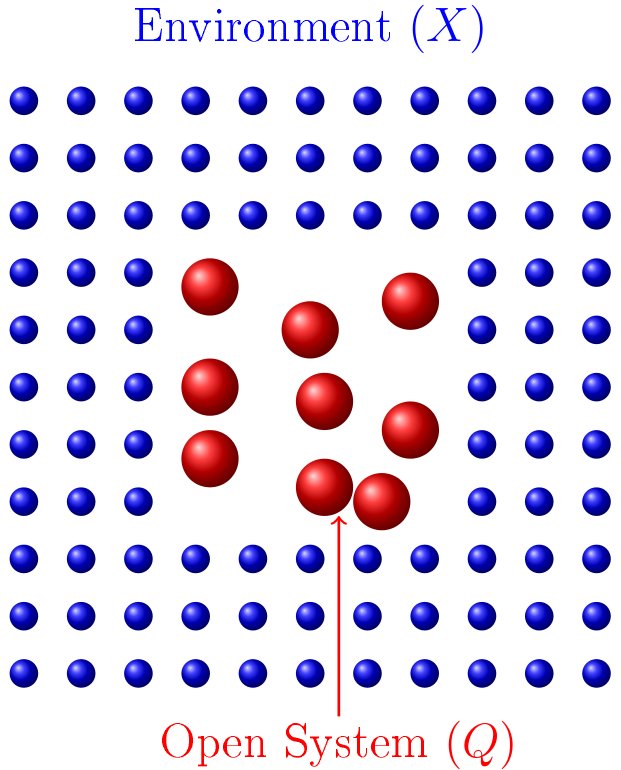
Consider a many-body phonon system of the type shown in Figure 1. It consists of a general central system (the open system), described by coordinates , acting under an arbitrary Hamiltonian . The secondary system (the environment) is composed of harmonic oscillators (with masses ) coupled both internally and with the open system. The open system may be subjected to time-dependent external fields. The environment uses displacement coordinates and the interaction between the two systems is linear in but arbitrary in :
| (4) |
This Hamiltonian differs from the standard CL Hamiltonian in Eq. (2) in two important respects. First, the interaction between the primary and secondary systems is no longer strictly bilinear, but can depend arbitrarily on . In addition, the atomic displacements that form the environment are now coupled to each other as well as the system, with the coupling described by the force-constant matrix . These alterations will have a material effect on our results. We also note the counter-term found in Eq. (2) has been dropped as it is no longer needed, since when the Hamiltonian of an arbitrary combined system is expanded in the power series in terms of atomic displacements , this kind of term does not appear. In this sense our model Hamiltonian is the second-order expansion of any conceivable system-bath Hamiltonian.
The density matrix evolves in the usual manner according to the Liouville equation:
| (5) |
where
| (6) |
is the corresponding evolution operator. Importantly we need not assume that the system Hamiltonian is time-independent. i.e. . The dynamics of the open system are found by tracing the full density matrix over the coordinates:
| (7) |
while the total and reduced density matrices in coordinate space are, respectively:
| (8) |
| (9) |
The propagators in this space are given by:
| (10) |
| (11) |
The second equality has been constructed to demonstrate that in coordinates, has the form of a backward propagation in time. Setting for convenience, the open system density matrix in the coordinate representation is:
| (12) |
At this point we transform to a normal mode representation , where
and are eigenvectors of the dynamical matrix , where , with eigenvalues . The eigenvectors satisfy the usual orthogonality, , and completeness, , conditions (the superscript stands for transpose). Applying these transformations, the Hamiltonian can be expressed as:
| (13) |
where
| (14) |
The reduced density matrix is now given by:
| (15) |
Before Eq. (15) can be solved, we must specify the form of the initial density matrix . As was explained in the Introduction, in most systems of interest the interaction between the primary system and its environment is an integral part of the system and hence one cannot assume the two systems are initially partitioned. One solution employed by Grabert et al. [54] is to consider the full interacting system as being allowed to equilibrate with some time-independent Hamiltonian before applying any time-dependent perturbation. In this case the initial state would then be described by the canonical density matrix:
| (16) |
where is the inverse temperature and is the corresponding partition function of the entire system. Note that a class of more general initial density matrices can be considered [54], however, here we shall limit ourselves only to the canonical density matrix.
III The Path Integral Representation and Influence Functional
To proceed we will insert the path integral representation of both propagators and the initial density matrix into Eq. (15). The expression for the forward propagator as a path integral up to a time is given by
| (17) |
with a similar definition for the backward propagator
| (18) |
The limits of the path integral in the second propagator are reversed as compared to the first one to emphasize its backward nature, as in Eq. (11).
In both expressions the integration is performed with respect to both the open system () and environment () variables between the boundaries indicated. Here is the action corresponding to the Hamiltonian in Eq. (13) describing the total system. It is defined in both propagators in the usual manner (i.e. the time integral of the Langrangian from to ), hence the extra negative in the exponent of the backwards propagator. Integration over the environmental variables can be performed exactly as the environment and interaction Hamiltonians added together have the form of a set of displaced harmonic oscillators in the environment variables. This means the path integral over environmental trajectories is Gaussian, and can be evaluated (see, e.g., [30, 29, 54]). The propagator therefore becomes a path integral over the trajectories of the open system only:
| (19) |
Here is a fluctuating factor that corresponds to a closed loop path integral:
| (20) |
while the action is the composition of the action of two systems, which is functionally dependent only on . Explicitly:
| (21) |
where is the open system action
| (22) |
and is the classical action of a set of displaced harmonic oscillators for an external “force” given by . This has no functional dependence on the coordinates; only depends on the limits of the path integral over the environment:
| (23) |
In the final equation above, we have abbreviated by setting , in addition to the limits and .
The backward propagator has a similar expression as compared to the forward propagator in Eq. (19):
| (24) |
with the same expression (21) for the action, but using the substitution . The abbreviation will also be used when referring to the backward propagator.
As well as the propagators, the initial density matrix may also be expressed as a path integral over both the open system and environmental coordinates. After performing the same integration over the environment as for the propagators, we obtain:
| (25) |
| (26) |
Here is the partition function for the total system, while is the Euclidean action, defined as the Wick rotation of . Using the notation , and , we obtain a familiar (albeit Wick rotated) definition for (see, e.g., [54]):
where the system and bath contributions are given as follows:
| (27) |
and
| (28) |
Following Ref. [54], we now also define a new partition function in terms of the partition functions of the total system and the (isolated) environment
| (29) |
After substituting the path integral and partition function expressions into Eq. (15), we obtain an expression for the reduced density matrix after integrating over the environmental trajectories:
| (30) |
The limits of the path integrals here are the same as above. The normalising constant in the equilibrium density operator is not generally known, and this issue will be discussed in Section V.
The influence functional contains the full path integral over the environment. It is fully factorised over the normal modes , and for each mode is composed of a product of three terms:
| (31) |
where
| (32) |
| (33) |
| (34) |
In order to calculate the influence functional, we notice that the calculation can be performed for each mode separately. Then, the integrand in the triple integral over , and contains an exponential function with a quadratic polynomial over these variables, and is hence a Gaussian. This can therefore be directly integrated. We first note that all pre-exponential factors in the influence functional after the integration multiply exactly to one. Indeed, the introduction of the partition function of the environment in Eq. (31) is to ensure that in the case of no interactions between the system and the environment, the influence functional is unity. If is the pre-exponential factor appearing after the triple integration over , and in Eq. (31) for one mode, then the overall exponential prefactor for the influence functional after some simple algebra is one:
| (35) |
After performing the complete integration of Eq. (31), we find the following exponential expression for the influence functional (cf. [29, 54]):
| (36) |
where is the influence phase:
| (37) |
The term multiplying the various within the integrals is the kernel:
| (38) |
Note that the kernel appears in three forms, depending on purely imaginary times, , real times, , and complex times, . It will be useful later in the derivation to split the kernel into its real and imaginary parts. For real times this produces,
| (39) |
| (40) |
and for complex times,
| (41) |
| (42) |
while for purely imaginary times the kernel is real,
| (43) |
and consisting of even and odd components:
| (44) |
| (45) |
If for real times we also define new sum and difference interaction functions [40],
| (46) |
and substitute these expressions into Eq. (37), the single mode influence phase can now be expressed as:
| (47) |
The final two terms in this expression are a generalisation of the well known Feynman-Vernon influence functional [29], with the remaining terms arising from the incorporation of a non-partitioned initial density matrix. Note that, compared to Eq. (37), the above expression was modified to ensure identical limits in the double integrals over the times and .
The influence phase still contains the normal mode interaction term . Using Eq. (14), we can re-express the phase in terms of the original interaction given in the site representation. The normal mode transformation did not change the coordinates themselves, so there is no difference between representations in the path integral measure or action in Eq. (30). The system-bath interaction term contained in the influence functional will have a different form however, and hence the influence phase has a non-trivial alternative representation in terms of functions rather than . In this representation the sum and difference functions
| (48) |
can conveniently be introduced, using . Substituting Eq. (14) into these, we can relate the sum and difference functions (46) between the normal mode and site representations:
| (49) |
The influence phase in the site representation is most easily expresed by defining new kernels from those derived using normal modes
| (50) |
| (51) |
| (52) |
| (53) |
so that the influence phase can be re-expressed in terms of the site interactions:
| (54) |
| (55) |
where an obvious short-hand notation has also been introduced.
The influence phase expressed here contains additional complexity compared to one derived using a standard CL model (which does not require a normal mode transformation) [54]. After allowing the environment to contain internal couplings, we find that the effect of this generalisation on the form of the influence phase is not trivial: instead of a single sum over the bath lattice in the CL model, we have double sums in Eq. (54), and this will have a profound effect on the dimensionality of the stochastic field to be introduced below.
In principle, having found the influence phase, Eq. (30) can be used to describe the exact dynamics of the open system at all times. Path integrals are however awkward to evaluate outside of certain special cases. The goal now is to use Eq. (30) to derive an operator expression, and hence a Liouville-von Neumann type equation for the reduced density matrix instead. Unfortunately the influence phase contains double integrals in two time variables ( and ), meaning there is no simple method to construct a differential equation directly out of Eq. (30). Here we will follow previous work [13, 40, 42, 46], and use a transformation to convert this non-local system into a local one exactly, at the cost of introducing stochastic variables.
IV The Two-Time Hubbard-Stratonovich transformation
In order to progress, we will use a statistical technique known as the Hubbard-Stratonovich (HS) transformation [57]. We shall consider the most general form of such a transformation based on a complex multivariate Gaussian distribution (cf. [46]).
Consider a Gaussian distribution over complex random variables (“noises”), , and their complex conjugates, :
| (56) |
where
| (57) |
is the vector of complex variables () or their conjugate (). The total vector is therefore of size and is given by:
The covariance matrix can also be decomposed into a block form
| (60) |
and the correlation functions are given by the usual Gaussian identity:
| (61) |
The Fourier transform of this distribution is the complementary distribution which can be calculated exactly:
| (62) |
where is a -fold vector, consisting of two size vectors and .
This equation can be interpreted as an average (with respect to the Gaussian distribution ) of the exponential function, . Using the distribution , one can also calculate the correlation function between any two stochastic variables. Hence, the elements of the inverse matrix appearing in Eq. (62) can be written via the correlation functions. The HS transformation is essentially the relation between these two representations of the complementary distribution:
| (63) |
So far, we have considered a finite set of discrete stochastic variables . The preceding derivation can be extended to (continuous) Gaussian stochastic processes if different stochastic variables are now associated with time instances separated by some small time interval , i.e. . Here with running from to , so that . Now in the limit of , we obtain the HS transformation for a set of continuous Gaussian stochastic processes as follows:
| (64) |
Note that integration over the noises appearing in both sides of the above equation, becomes the corresponding path integral in the continuum limit.
Using the HS transformation defined above, clear progress can be made. Indeed, the exponent in the right hand side of Eq. (64) is of the same form as the Feynman-Vernon terms of the influence phase in Eq. (55). The correlation functions and variables in Eq. (64) can be mapped to the terms appearing in the integrands of the Feynman-Vernon influence phase. The HS transformation can therefore be used to equate a deterministic non-local integral exponent to a local phase involving auxiliary stochastic terms, that must be averaged over the distribution . In a more physical sense, we can also consider the HS transformation as converting a system of two body potentials into a set of independent particles in a fluctuating field. The difficulty using this transformation is that Eq. (55) contains two time dimensions - one real and one imaginary, with one term involving an integration over both dimensions - requiring a generalisation of the transformation.
When we consider how the HS transformation is derived, continuous processes and multiple variables are incorporated through the addition of extra indices, partitioning the arbitrary sum of random complex variables. The same procedure can be applied to introduce different time dimensions. Starting from a discrete representation, we introduce two sets of times, and , so that the exponent on the left hand side of the HS transformation (63) has the form
| (65) |
where we assign and , and we place a bar above quantities associated with the second set of times (denoted with the real time ). Note that the number of stochastic variables in each set (as counted by the index for the given time index ) may be different for barred and unbarred fields. In the continuum limit we obtain for the left hand side of the HS transformation:
| (66) |
Correspondingly, the exponent on the right hand side of Eq. (63) (after the time labels are introduced), in the continuous limit becomes:
| (67) |
where, because of the three possible combinations of times, we introduce three types of correlation functions:
| (68) |
| (69) |
| (70) |
In the full multivariate form, the two-time transformation is therefore given by:
| (71) |
The connection between the influence phase and the two-time Hubbard-Stratonovich transformation should now be transparent. Notice that here in the exponential all time integrals have either or as their upper limits, exactly as in the influence functional expression (55) for the phase. The choice for the second time dimension to run up to has been made to highlight the closeness between the influence phase in Eq. (55) and the two-time HS transformation presented here.
Now we would like to apply the HS transformation to the influence functional expression given by Eqs. (36), (54) and (55). It is clear from the structure of the exponent in the influence functional in Eq. (55), that auxiliary stochastic fields should be introduced separately for each lattice site index . Moreover, there should be two pairs of the stochastic processes for the set associated with the real time ,
and one such set for the imaginary time :
| (76) |
where we have redefined the size (number of environmental oscillators) complex vector to include two noises and their conjugates. Next, we make the following correspondence between the functions in the HS transformation (71) and the functions , and appearing in the phase, Eq. (55):
| (77) |
and
| (78) |
The three pairs of stochastic processes we have introduced must ensure that the influence functional given by Eqs. (36), (54) and (55) coincides exactly with the right hand side of the HS transformation (71). Therefore, comparing the exponents in the right hand side of Eq. (71) and Eq. (55), explicit formulas can be established for the correlation functions between the noises. These are:
| (79) |
| (80) |
| (81) |
| (82) |
| (83) |
Note that the correlation functions (79) and (82) are to be symmetric functions with respect to the permutation and , respectively, and the corresponding functions and provide exactly this.
Taking the above results and applying them to Eq. (55), we find that the influence functional can be described as an average over multivariate complex Gaussian processes as follows:
| (84) |
where the averaging is made over three pairs of complex noises (or, equivalently, over six real noises) per lattice site of the environment.
Importantly, the two-time HS transformation is a purely formal one, and we are free to stipulate that the noises are pure C-numbers; this enables us to avoid the complication of operator-valued noises. Promoting noises to operators has been previously shown to have no effect on the final result, as shown in Ref. [40, 42].
Finally it is worth mentioning that the influence phase given above does not uniquely define the Gaussian processes that the influence functional is averaged over after performing the mapping. The influence phase viewed as the right hand side of the HS transformation does not involve every possible correlation defined under the Gaussian distribution. In particular, the conditions we impose on some correlation functions to map the physics to the auxiliary noises do not constrain the correlations between the complex conjugate noises, e.g. . Therefore any distribution that satisfies Eqs. (79-83) may be used in this transformation.
V The Extended Stochastic Liouville-von Neumann Equation
Now the influence functional has been evaluated, we are able to write the expression for the reduced density matrix in Eq. (30) explicitly. First, having introduced stochastic variables into the equation for the density matrix, we must define a new object to act as an effective, single-trajectory density matrix defined for a particular realisation of the stochastic processes and along its path. Inserting Eq. (84) into Eqn.(30) we obtain:
| (85) |
so that the exact reduced density matrix is recovered as an average over all noises:
| (86) |
Above three effective actions have been introduced:
| (87) |
| (88) |
| (89) |
In the definitions of the effective actions we have reinserted the original forces , and via Eq. (48). It can be seen that the actions and correspond to two different effective Lagrangians,
| (90) |
which in turn are associated with two different effective Hamiltonians:
| (91) |
As was mentioned in Section IV, the noises are not promoted to operators but remain as -numbers.
All three path integral coordinates have now been decoupled from each other, and as coordinate functionals may be commuted. The density matrix in Eq. (85) can therefore be expressed as:
| (92) |
where
| (93) |
| (94) |
| (95) |
Notice that the forwards propagator is not the Hermitian conjugate of the backwards propagator because of the obvious difference in the their respective Hamiltonians. The consequence of this is that the equation of motion is no longer of the Liouville form, i.e. the time derivative of the density matrix is not solely given by the commutator with some kind of Hamiltonian.
| (96) |
| (97) |
which correspond to the forward and backward propagation performed with the different Hamiltonians and , respectively, with the corresponding chronological and anti-chronological time-ordering operators. It is easy to see that the coordinate representation and of such operators give exactly the paths integrals in these expressions. The propagator operators satisfy the usual equations of motion
| (98) |
| (99) |
Taking Eqs. (92)-(95), the reduced single-trajectory density matrix of the open system can be written as an operator evolution:
| (100) |
With these definitions it is possible to generate an equation of motion for a single-trajectory reduced density matrix by simply differentiating the above expression with respect to time:
| (101) |
This, together with an equation for , which provides an initial condition for the reduced density operator , forms the ESLN. It bears a great deal of similarity to the equation derived by Stockburger [46] using the partitioned approach, and while it may be initially surprising to see a similar (albeit generalised) equation of motion, it seems that the partition-free initial density matrix introduced here does not change the dynamics it evolves under. We also note that, as was mentioned above, the obtained equation does not have the usual Liouville form because of an extra anti-commutator term in the right hand side. This originates from the fact that the forward and backward propagations of the reduced density matrix in Eq. (100), are governed by different Hamiltonians. We note that the same equation of motion for the reduced density matrix can also be obtained using the method developed by Kleinert and Shabanov in Ref. [40]. However, their method requires some care in choosing the correct order of the coordinates and momenta operators. It is a definite advantage of our method that such a problem does not arise.
All that remains is to determine the new single-trajectory initial density matrix . This is the true initial () single-trajectory reduced density matrix which is obtained from the canonical density matrix (16) by tracing out the degrees of freedom of the bath. There is already a path integral representation for this density, Eq. (95), but it is unwieldy and unintuitive. Once again it is best to work backwards to obtain the corresponding effective canonical initial density matrix operator with the same path integral representation. It is easy to see, however, considering an effective operator Hamiltonian, cf. Eq. (89),
| (102) |
that the path integral representation of the initial density matrix in Eq. (95) is formally identical to the one for the coordinate representation of the evolution operator when time is imaginary and changes between zero and . Therefore, the initial reduced density operator can be characterised as a propagator through imaginary time:
| (103) |
using
| (104) |
This has the form of a time-ordered exponent with being the corresponding chronological time-ordering operator. The latter density operator is responsible for the thermalisation of the open system (when ) and will be called the quenched initial density operator. It satisfies the Schrödinger-like equation of motion
| (105) |
with the initial condition . The initial density must be normalised when the final value of is reached, i.e. , where the trace is taken with respect to the open system only. Therefore, the correct initial condition for can be fixed by providing this normalisation at the end of the imaginary time propagation (note that , as a ratio of two partition functions, is time independent). We also observe that essentially the same result for the reduced equilibrium density matrix was obtained in Ref. [56].
The Hamiltonian and the interaction operators in have no temperature dependence; so the temperature dependence comes entirely from an artificial “propagation” of the quenched density matrix from zero to the “time” . This hard limit relating the time to the system temperature is important, as unlike in the real time case, the quenched density matrix may diverge as we take . This is a reflection of the fact that the path integral description of the canonical density matrix is itself only defined for finite temperature.
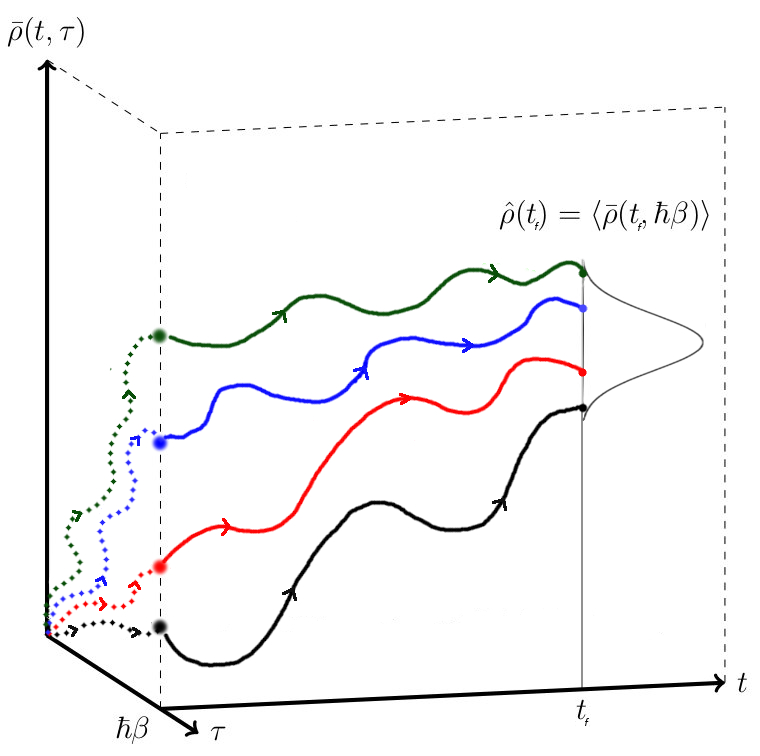
The equations (101), (103) and (105) provide the complete solution for the real time evolution of the reduced density matrix of an open system in our partition-free approach. First of all, the initial density matrix is obtained by propagating in imaginary time the quenched density up to the final time (the Euclidean evolution). The initial density is then normalised which fixes the value of the partition function . Using the obtained initial density matrix, the actual time dynamics of the reduced density matrix are elucidated by solving Eq. (101). Figure 2 illustrates the evolution of trajectories through two times, as governed by the two differential equations. First the system evolves through imaginary time according to Eq. (105) and some realisation of the imaginary time noise trajectory . This state then evolves through real time under Eq. (101) using the real time noise trajectories and , with the requirement that upon averaging over realisations of these trajectories, they satisfy the correlation functions derived in section IV. The evolution along these two time dimensions is then repeated many times using various realisations of the stochastic noises, and averaging over many trajectories yields the physical reduced density matrix appearing in Eq. (86).
VI Discussion and conclusions
Having derived the ESLN, we should ask how it differs from previous work. The Hamiltonian we have used is a generalisation of the Caldeira-Leggett model, allowing for a solution in either real or frequency space. The form of the interaction has also been generalised, but is still limited by the essential need for an interaction to be linear in environmental oscillator displacements. In fact, our Hamiltonian emerges naturally from an arbitrary total system Hamiltonian by expanding atomic displacements of the environment up to the second order. Therefore, it can be directly applied to realistic systems.
The fundamental result of our paper is the removal of the unphysical partitioned initial condition which implied that the open system and the bath were initially isolated. Following previous procedures to accommodate a more physical partition-free approach, we applied the special variant of the Hubbard-Stratonovich transformation that allowed the initial condition to be determined via an auxiliary differential equation. This allows the ESLN to make exact predictions for the transient behaviour of the primary system when it is perturbed from equilibrium. Additionally, when the total system is in equilibrium, the imaginary time differential equation allows for the exact calculation of the reduced equilibrium density matrix. This is important, as the stationary distribution of dissipative systems with finite couplings has been shown to deviate from that expected under partitioned conditions [58]. The true distribution is described by the “Hamiltonian of mean force”, and Eqs. (103) and (105) provide a route to the exact calculation of the stationary distribution. Indeed, the imaginary time evolution has been independently derived by Moix et al. [56] as an exact description of an open system in interactive equilibrium with its environment. This formulation of the equilibrium density matrix has been used by Tanimura to develop hierarchical equations of motion for fermionic systems [59] under the assumption that the environment spectral density is Ohmic.
The ESLN represents a unification and generalisation of the differential equations derived by Stockburger [46] and Moix et al. [56], resulting in additional and highly non-trivial constraints on the correlations between the real and imaginary time noises. The connection between these two pieces of work was not previously apparent, but has emerged naturally from the simultaneous generalisation of the model Hamiltonian and the initial total density matrix. This is the ESLN’s principal advantage, and allows for a simpler and more general closed form description of the evolution of the reduced density matrix, as compared to hierarchical equations of motion [59]. We also note that our approach can easily be generalised to several environments, e.g., for heat transport problems along similar lines to Ref. [21].
Extracting numerical results from the ESLN depends on the feasibility of generating noises that satisfy the correlations outlined in section IV. Real time noises of the same type can already be efficiently calculated [46], and the outlook for extending this to include the imaginary time noise is promising. Looking forward, a first application of the ESLN is therefore likely to be a calculation of the time evolution of the density matrix for a simple system coupled to a harmonic bath, and the comparison between approximate partitioned and exact partition-free methods.
The class of problems that this model may be applied to are rather broad. This includes a two-level spin boson system, coupled to a bath with an arbitrary spectrum [46], or the heat exchange between an arbitrary system and a bath with Ohmic dissipation [45]. It is possible that this generalisation may also be applied to numerical schemes for anharmonic bath models [60], and influence functional simulations of complex systems [61].
To summarise, the influence functional formalism has been used to generate two stochastic differential equations that together describe the exact evolution of an open system that begins in coupled equilibrium with its harmonic environment. The results presented here are an extension to existing frameworks for thermodynamic analysis in the quantum regime, as well as offering a method for accessing the equilibrium states of arbitrary dissipative systems.
Acknowledgements
The authors would like to thank Prof Ulrich Weiss for his help in verifying the Feynman-Vernon influence phase at the early stages of this work. GMG is supported by the EPSRC Centre for Doctoral Training in Cross-Disciplinary Approaches to Non-Equilibrium Systems (CANES, EP/L015854/1). We also would like to thank Ian Ford and Claudia Clarke for thought-provoking and stimulating discussions.
References
- [1] I. J. Ford. New J. Phys 17(7), 075017, (2015).
- [2] U. Weiss. Quantum dissipative systems. (World Scientific, Singapore, 2009).
- [3] P. Hänggi, P. Talkner, and M. Borkovec. Rev. Mod. Phys, 62, 251, (1990).
- [4] V.I. Melnikov. Physics Reports, 209(1), 1, (1991).
- [5] K.W.H. Stevens. Proc. Phys. Soc, 72(6), 1027, (1958).
- [6] E. Kerner. Canadian J. Phys., 36(3), 371, (1958).
- [7] E. Kanai. Prog. Th. Phys, 3(4), 440, (1948).
- [8] I.R. Senitzky and A. Rutherford. Phys. Rev, 119(2), 670, (1960).
- [9] H. B. Callen and T.A. Welton. Phys. Rev, 83(1), 34, (1951).
- [10] M. Lax. Phys. Rev, 129(5), 2343, (1963).
- [11] G. W. Ford, M. Kac, and P. Mazur. J. Math. Phys, 6(4), 504, (1965).
- [12] R. Benguria and M. Kac. Phys. Rev. Lett, 46(1), 1, (1981).
- [13] A. Schmid. J. Low. Temp. Phys, 49(5-6), 609, (1982).
- [14] K. Lindenberg and B. J. West. Phys. Rev. A, 30(1), 568, (1984).
- [15] E. Cortes, B. J. West, and K. Lindenberg. J. Chem. Phys, 82(6), 2708, (1985).
- [16] A.O. Caldeira and A.J. Leggett. Physica A, 121(3), 587, (1983).
- [17] M. Rosenau da Costa, A.O. Caldeira, S.M. Dutra, and H. Westfahl. Phys. Rev. A, 61, 022107, (2000).
- [18] L. Kantorovich. Phys. Rev. B, 78, 094304, (2008).
- [19] L. Stella, C. D. Lorenz, and L. Kantorovich. Phys. Rev. B, 89, 134303, (2014).
- [20] H. Ness, L. Stella, C. D. Lorenz, and L. Kantorovich. Phys. Rev. B, 91, 014301, (2015).
- [21] H. Ness, A. Genina, L. Stella, C.D. Lorenz, and L. Kantorovich. Phys. Rev. B, 93, 174303, (2016).
- [22] L. Kantorovich, H. Ness, L. Stella, and C.D. Lorenz. Phys. Rev. B, 94, 184305, (2016).
- [23] P. Hänggi. Z. Phys. B, 68(2), 181, (1987).
- [24] H. Grabert, P. Olschowski, and U. Weiss. Phys. Rev. B, 36(4), 1931, (1987).
- [25] E. Pollak. Phys. Rev. B, 40(4), (1989).
- [26] I. Affleck. Phys. Rev. Lett, 46(6), 388, (1981).
- [27] J. O. Richardson, R. Bauer, and M. Thoss. J. Chem. Phys, 143(13), 134116, (2015).
- [28] J. O. Richardson. J. Chem. Phys, 144, 114106, (2016).
- [29] R. P. Feynman and F. L. Vernon. Ann. Phys, 24, 118, (1963).
- [30] R.P. Feynman and A.R. Hibbs. Quantum Mechanics and Path Integrals. (Dover, New York, 2010).
- [31] J.S. Schulman. Techniques and Applications of Path Integration. (Dover, New York, 1981).
- [32] C. M. Smith and A.O. Caldeira. Phys. Rev. A, 36(7), 3509, (1987).
- [33] N. Makri. Chem. Phys. Lett, 159(5,6), 489, (1989).
- [34] K. Allinger and M. A. Ratner. Phys. Rev. A, 39(2), 864, (1989).
- [35] G. W. Ford and M. Kac. J. Stat. Phys, 46. 803, (1987).
- [36] C. W. Gardiner. IBM J. Res. Develop, 32, 127, (1988).
- [37] K. L. Sebastian. Chem. Phys. Lett, 81(1), 14, (1981).
- [38] A. J. Leggett, S. Chakravarty, A. T. Dorsey, M. Fisher, A. Garg, and W. Zwerger. Rev. Mod. Physics, 59(1), 1, (1987).
- [39] N. G. van Kampen. J. Molec. Liquids, 71, 97, (1997).
- [40] H. Kleinert and S. V. Shabanov. Phys. Lett. A, 200(3-4), 224, (1995).
- [41] H. Kleinert. Path Integrals in Quantum Mechanics , Statistics , Polymer Physics and Financial Markers. (Berlin, 3rd edition, 2006).
- [42] K. Tsusaka. Phys. Rev. E, 59(5 Pt A), 4931, (1999).
- [43] C. Bhadra and D. Banerjee. J. Stat. Mech, 2016(4), 043404, (2016).
- [44] H. Keith McDowell. J. Chem. Phys, 112(16), 6971, (2000).
- [45] M. Carrega, P. Solinas, A. Braggio, M. Sassetti, and U. Weiss. New J. Phys, 17(4), 045030, (2015).
- [46] J. T. Stockburger. Chem. Phys, 296, 159, (2004).
- [47] D. Banerjee, F. Hebenstreit, F. Jiang, M. Kon, and U. Wiese in The 33rd International Symposium on Lattice Field Theory: Kobe, Japan, June 2015.
- [48] N. Makri. Chem. Phys. Lett, 593, 93, (2014).
- [49] N. Makri. J. Chem. Phys, 109(8), 2994, (1998).
- [50] N. S. Dattani, F. A. Pollock, and David M. Wilkins. Quant. Phys. Lett, 1(1), 35, (2012).
- [51] S. Habershon, D. E. Manolopoulos, T. E. Markland, and T. F. Miller. Ann. Rev. Phys. Chem, 64, 387, (2013).
- [52] C. P. Herrero and R. Ramírez. J. Phys. Cond. Mat, 26, 233201, (2014).
- [53] J. Wang. Phys. Rev. Lett, 99(16), 160601, (2007).
- [54] H. Grabert, P. Schramm, and G. Ingold. Phys. Rep., 168(3), 115, (1988).
- [55] R. Karrlein and H. Grabert. Phys. Rev. E, 55(1), 153, (1997).
- [56] J. M. Moix, Y. Zhao, and J. Cao. Phys. Rev. B, 85(11), 1, (2012).
- [57] R.L. Stratonovich. Doklady Phys, 115, 1097, (1958).
- [58] S. Hilt, B. Thomas, and E. Lutz. Phys. Rev. E, 84, 031110, (2011).
- [59] Y. Tanimura. J. Chem. Phys., 141(4), (2014).
- [60] N. Makri. J. Phys. Chem. B, 103(15), 2823, (1999).
- [61] P. L. Walters and N. Makri. Phys. Chem. Lett., 6(24), 4959, (2015).