Projection Pursuit for non-Gaussian Independent Components Thanks: Joni Virta is PhD student, University of Turku, 20014, Finland (E-mail: joni.virta@utu.fi). Klaus Nordhausen is Postdoctoral Researcher, University of Turku, 20014, Finland (E-mail: klaus.nordhausen@utu.fi). Hannu Oja is Professor Emeritus, University of Turku, 20014, Finland (E-mail: hannu.oja@utu.fi). This work was supported by Academy of Finland (grant 268703). The authors wish to thank Jari Miettinen who provided the code used for the comparison of the individual signal estimates in Section 6.Thanks: This work is partially based on the unpublished manuscript Virta et al. (2015) available as an arXiv preprint, arXiv:1505.02613.

The basic blind source separation (BSS) model assumes that the observed random vectors $\textbf{x}_{i}\in\mathbb{R}^{p}$ are linear combinations of some unobservable random vectors $\textbf{z}_{i}\in\mathbb{R}^{p}$, $i=1,\ldots,n$, the estimation of which is the main objective. This can be formalized as

where $\boldsymbol{\mu}$ is a location shift and $\boldsymbol{\Omega}\in\mathbb{R}^{p\times p}$ is a non-singular mixing matrix. In independent component analysis (ICA) it is further assumed that the random vector $\textbf{z}_{i}$ has mutually independent and standardized components and that at most one of the components is normally distributed. The constraint on non-Gaussianity is needed as otherwise the rotational invariance of the standard multivariate Gaussian distribution makes the model ill-defined. For an overview of ICA and BSS models, see e.g. Comon and Jutten (2010).

However, if it is reasonable to assume the existence of more than one source of noise it might be too strict to restrict the number of Gaussian components to at most one. In the so-called non-Gaussian component/subspace analysis (NGCA) (Blanchard et al., 2005) the assumptions in the model (1) are relaxed by allowing more sources of Gaussian noise. That is, as formulated in Theis et al. (2011), one assumes that for some $d$, $0\leq d\leq p$ the vector $\textbf{z}_{i}$ consists of a $d$-dimensional non-Gaussian subvector (that spans the signal space) and a $(p-d)$-dimensional Gaussian subvector (that spans the noise space) that are independent of each other. In this model the signal and the noise subspaces are well defined and estimable but the individual components are not. A further distinctive property of NGCA is that the dimension of the signal subspace is usually assumed to be known. For other related or similar models, see Bonhomme and Robin (2009), Comon and Jutten (2010), Woods et al. (2015) and Risk et al. (2015).

In this paper we combine the ICA and NGCA approaches and require that in (1) exactly $p-d$ of the mutually independent components of $\textbf{z}_{i}$ are Gaussian. The objective is then to estimate the signal and noise subspaces (as in NGCA) as well as the individual signal components (as in ICA). In the estimation we use projection pursuit (PP) with convex combinations of squared third and fourth cumulants as projection indices. We derive the properties of the estimates assuming that $d$ is known, but also discuss its estimation in Section 7.

Projection pursuit is a popular method that finds hidden structures in multivariate data by searching for one- or low-dimensional projections of interest. This is done by finding projections that maximize the value of an objective function, the so-called projection index. The classical measures of skewness and kurtosis, the third and fourth moments of a random variable after standardization, have been widely used for this purpose. Huber (1985) considered various projection indices with heuristic arguments that non-Gaussian linear combinations are the most interesting. His indices were ratios of two dispersion functionals thus measuring kurtosis with the classical kurtosis measure as a special case. Peña and Prieto (2001) used projection pursuit for hidden cluster identification with the classical kurtosis measure. For early contributions on projection pursuit see also Friedman and Tukey (1974) and Jones and Sibson (1987).

In the engineering literature Hyvärinen and Oja (1997) were the first to propose a projection pursuit approach for independent component analysis with the absolute value of the excess kurtosis, the fourth cumulant of a standardized random variable, as the projection index and considered later an extension with a choice among several alternative measures of non-Gaussianity, including the absolute value of the classical skewness, the third cumulant of a standardized random variable. The approach is called deflation-based FastICA or symmetric FastICA depending on whether the independent components are estimated one-by-one or simultaneously, respectively. These two versions of FastICA can actually be seen as the optimization of different norms of the same vector of component-wise criterion values, namely the repeated maximization of $L_{\infty}$-norm and the maximization of $L_{1}$-norm, respectively. In this paper we choose however to work with the $L_{2}$-norm, firstly because of its analytical tractability over other choices of $L_{p}$-norms, and secondly because of its connection to the popular JADE estimate, see Corollary 5.2. The deflation-based approach also has the useful property that under our model the estimation of each sequential component can be seen as a test for normality, allowing us to do inference on the dimension $d$ of the signal subspace, see Section 7. Although the use of the $L_{2}$-norm was mentioned already in Hyvärinen (1999) and Comon and Jutten (2010) the idea was not carried any further. For recent discussions of FastICA methods, see Ollila (2010), Nordhausen et al. (2011), Miettinen et al. (2014), Miettinen et al. (2015), Wei (2015). For other classical approaches to ICA, see e.g. Cardoso (1989), Cardoso and Souloumiac (1993) and the application of the latter to NGCA in Kawanabe (2005).

In the engineering literature the ICA procedures are often seen more as numerical algorithms than as estimates of certain population quantities and considering their statistical properties is usually neglected. Recently, however, also more statisticians have become interested in the problem. Chen and Bickel (2006) and Samworth and Yuan (2012), for example, developed estimates that need only the existence of first moments and rely on efficient nonparametric estimates of the marginal densities. Efficient estimation methods based on residual signed ranks and residual ranks have also been developed recently by Ilmonen and Paindaveine (2011) and Hallin and Mehta (2015). For other approaches see also, for example, Karvanen and Koivunen (2002); Hastie and Tibshirani (2003); Matteson and Tsay (2016).

Regarding signal separation, one limitation to the previously discussed methods is set by the measure of non-Gaussianity itself; if some signal component has a distribution with the same criterion value as the normal distribution (usually zero) it is treated as noise. This is where the benefits of our preferred approach show the most; jointly using both third and fourth cumulants means that the signal components can have either zero skewness or zero excess kurtosis and still be estimated. Furthermore, we show that the method is Fisher consistent under suitable moment conditions. Theoretically any number of univariate cumulants of order three or higher could be used together to find the non-Gaussian signals, see Moreau (2001).

The joint use of third and fourth cumulants in ICA-type problems has also been previously discussed in the literature: Jones and Sibson (1987) approximate the entropy of a distribution suitably close to the Gaussian distribution with a particular weighted sum of squared skewness and excess kurtosis, a special case of the projection index we use, see also Amari et al. (1996) for similar constructions; Karvanen and Koivunen (2002); Karvanen et al. (2002) use the method of moments to estimate the source score functions either from Pearson’s system of distributions or the extended generalized lambda distribution (EGLD) by matching moments (or L-moments) up to the fourth; Karvanen and Koivunen (2004) propose using a weighted sum of the absolute values of skewness and excess kurtosis as an objective function in minimization of mutual information; Comon and Rajih (2006) used the characteristic function to solve an independent component problem with more latent variables than observed variables; Li et al. (2011) proposed using a joint diagonalization of second or higher order cumulant matrices in the context of joint blind source separation (JBSS) and Comon et al. (2015) considered the simultaneous decomposition of multiple symmetric tensors of different orders.

The paper is structured as follows; we begin in Section 2 by providing some notation. Section 3 introduces the model along with the relevant assumptions and also discusses the concepts of signal separation functionals and affine equivariance. Sections 4 and 5 then consider the estimation of the signals both separately and simultaneously via projection pursuit with the previously unexplored use of the $L_{2}$-norm. A thorough discussion is provided including also the asymptotic behaviors of both considered methods. In Sections 6 and 7 the presented procedures are compared in their ability to extract single signals and the entire signal subspace. In the latter some thought on estimating the value of $d$ is also given. We end with some discussion on the results and prospective work in Section 8. The proofs are reserved for the Appendix.

The simulations and computations were performed using R 3.2.3 (R Core Team, 2015) and additionally the packages clue (Hornik, 2016), ggplot2 (Wickham, 2009), ICS (Nordhausen et al., 2008), JADE (Nordhausen et al., 2015), Rcpp (Eddelbuettel and François, 2011) and RcppArmadillo (Eddelbuettel and Sanderson, 2014).

For a univariate random variable $x$, we write $x_{st}:=(x-E(x))/\sqrt{Var(x)}$ for its standardized version. The classical skewness, kurtosis and excess kurtosis of $x$ are then

Note that the measures $\gamma(x)$ and $\kappa(x)$ are the third and fourth cumulants of the standardized variable $x_{st}$. For symmetric random variables $\gamma(x)=0$ and for the normal distribution $\kappa(x)=0$.

Throughout the paper we assume that $\textbf{z}_{1},\ldots,\textbf{z}_{n}$ is a random sample from a $p$-variate distribution of z with $E(\textbf{z})=\mathbf{0}$ and $Cov(\textbf{z})=\textbf{I}_{p}$ and that the $p$ components of z are mutually independent. As the methods considered are essentially moment-based we use, for all $k=1,\ldots,p$, the following shorthands for marginal moments.

Assuming a fixed weight parameter $\alpha\in[0,1]$, we will see in Sections 4 and 5 that the previous moments act as building blocks for the following asymptotic variances of the elements of our unmixing matrix estimates.

where $\alpha_{1}:=3\alpha$, $\alpha_{2}:=4(1-\alpha)$, $\zeta^{(3)}_{k}=\gamma_{k}^{2}(\nu_{k}-\gamma_{k}^{2})$, $\zeta^{(4)}_{k}=\kappa_{k}^{2}(\omega_{k}-\beta_{k}^{2})$ and $\zeta^{(34)}_{k}=\gamma_{k}\kappa_{k}(\eta_{k}-\gamma_{k}\beta_{k})$. The expressions $A_{k}$, $B_{kl}$ and $D_{k}$ are encountered in Theorems 4.2 and 5.2.

We write $F_{\textbf{x}}$ for the cumulative distribution function (c.d.f.) of a $p$-variate random vector x. Then $F_{\textbf{A}\textbf{x}+\textbf{b}}$ is the c.d.f. of $\textbf{A}\textbf{x}+\textbf{b}$. If the random vector x has the mean vector $\boldsymbol{\mu}$ and the covariance matrix $\boldsymbol{\Sigma}$, the standardized vector $\textbf{x}_{st}$ is given by $\textbf{x}_{st}:=\boldsymbol{\Sigma}^{-1/2}(\textbf{x}-\boldsymbol{\mu})$, where $\boldsymbol{\Sigma}^{-1/2}$ is chosen as the unique symmetric matrix G satisfying $\textbf{G}\boldsymbol{\Sigma}\textbf{G}^{T}=\textbf{I}_{p}$. Multivariate standardization is affine equivariant up to rotation, that is, if $\textbf{x}^{*}=\textbf{A}\textbf{x}+\textbf{b}$, then $(\textbf{x}^{*})_{st}=\textbf{V}\textbf{x}_{st}$, for some orthogonal matrix $\textbf{V}\in\mathbb{R}^{p\times p}$, see e.g. Ilmonen et al. (2012). This result is crucial in proving the affine equivariance of the signal separation functionals later on.

Fixing $\alpha\in[0,1]$, the projection pursuit methods in the following sections are based on the objective function

where x is the observed random vector and $\textbf{u}^{T}\textbf{u}=1$. For the estimating equations we further need its gradient,

Some often encountered sets of square matrices include the set of all orthogonal matrices, the set of all heterogeneous sign-change matrices (diagonal matrices with diagonal elements equal to $\pm 1$), the set of all heterogeneous scaling matrices (diagonal matrices with positive diagonal elements) and the set of all permutation matrices denoted, respectively, by $\mathcal{U},\mathcal{J},\mathcal{D}$ and $\mathcal{P}$. The set of all $d\times p$ matrices with orthonormal rows is denoted by $\mathcal{U}^{d\times p}$ and the equivalence relation $\textbf{A}\equiv\textbf{B}$ means that $\textbf{A}=\textbf{P}\textbf{J}\textbf{B}$, for some $\textbf{P}\in\mathcal{P}$, $\textbf{J}\in\mathcal{J}$. Also, let $\mathcal{C}$ denote the set of all matrices that can be expressed as JDP where $\textbf{J}\in\mathcal{J}$, $\textbf{D}\in\mathcal{D}$ and $\textbf{P}\in\mathcal{P}$.

The norm $\|\cdot\|$ refers for vector arguments to the standard Euclidean norm and for matrix arguments to the Frobenius norm.

The model used throughout the paper is the following combination of the ICA and NGCA models in which the $p$-variate observations $\textbf{x}_{1},\ldots,\textbf{x}_{n}$ are thought to be independent realisations of the random vector $\textbf{x}\in\mathbb{R}^{p}$ generated as

We further assume that the unobserved random vector z satisfies the following two assumptions.

The standardization conditions $E(z_{k})=0$ and $E(z_{k}^{2})=1$, $k=1,\ldots,p$, implied by Assumption 1 serve as identification constraints for the location $\boldsymbol{\mu}$ and the scales of the columns of $\mathbf{\Omega}$, implying that $E(\textbf{x})=\boldsymbol{\mu}\ \ \mbox{and}\ \ Cov(\textbf{x})=\boldsymbol{\Sigma}=\boldsymbol{\Omega}\boldsymbol{\Omega}^{T}$. Writing $\boldsymbol{\Omega}=(\boldsymbol{\Omega}_{1},\boldsymbol{\Omega}_{2})$ the model can also be expressed as

where $\boldsymbol{\Omega}_{2}\in\mathbb{R}^{p\times(p-d)}$ can be identified only up to a rotation from the right-hand side. The matrix $\boldsymbol{\Omega}_{1}\in\mathbb{R}^{p\times d}$, however, can be identified up to the signs and permutation of its columns, a fact which follows from the classical Skitovich-Darmois theorem restated here as Theorem 3.1, see Theorem 1 in Ibragimov (2014). The proof of Corollary 3.1 is given in the Appendix.

Assumption 2 quantifies our prior knowledge on the dimensions of the non-Gaussian signal subspace and the Gaussian noise subspace. Inference, testing and estimation of the dimension of the signal subspace is also briefly discussed in Section 7. In addition to Assumptions 1 and 2, for the limiting distributions of our unmixing matrix estimates to exist the existence of some higher moments of z is further required, see Theorems 4.2 and 5.2.

In the case of $d=0$ we simply get a multivariate normal model without any signal s and if $d=p-1$ or $d=p$ one gets the basic independent component model. Another related model is the so-called noisy independent component model, $\textbf{x}=\mathbf{\Omega}\textbf{s}+\textbf{n}$, with $d$ non-Gaussian independent components in s and Gaussian noise in the $p$-variate n with $\mathbf{\Omega}\in\mathbb{R}^{p\times d}$. Stacking the signal and noise parts to a single vector, the effective mixing matrix $(\boldsymbol{\Omega}|\textbf{I})$ is then non-square and standard ICA methods no longer apply. For such models, see e.g. Bonhomme and Robin (2009) and Comon and Jutten (2010).

Our approach for estimating the signal components and the signal subspace is projection pursuit with a preliminary step advised by the following theorem. The theorem is one of the key results of independent component analysis, see for example Miettinen et al. (2015) for its proof.

Theorem 3.2 essentially states that the estimation of the relevant rows of $\boldsymbol{\Omega}^{-1}$ can, using standardization, in fact be reduced to a simpler problem, namely to the estimation of a matrix U with orthonormal rows, and this is the task we use projection pursuit in the next sections for. Having estimated U a transformation into the signal space is then given by $\textbf{x}\mapsto\textbf{W}\textbf{x}$, where $\textbf{W}:=\textbf{U}\boldsymbol{\Sigma}^{-1/2}$.

Next, we give the definition of a signal separation functional which formalizes the role of the transformation matrix W above.

The condition $(i)$ in the definition above states that signal separation functionals are up to sign and permutation Fisher consistent to the $d$ rows of $\boldsymbol{\Omega}^{-1}$ corresponding to the signals. Note that this invariance with respect to signs and order is unavoidable since neither is fixed in the model (4). The condition $(ii)$ implies in particular that if we consider $F_{n}$, the empirical distribution function of a random sample $\textbf{x}_{1},\ldots,\textbf{x}_{n}$ from $F$, the estimate $\textbf{W}(F_{n})$ is also affine equivariant. This gives us the practical advantage of needing to consider only the case of identity mixing, $\boldsymbol{\Omega}=\textbf{I}_{p}$, when discussing the estimates’ asymptotic behaviors, the case of general $\boldsymbol{\Omega}$ easily following.

The requirement of affine equivariance further means that in the case of $d=p$ any signal separation functional $\textbf{W}(F)$ is also an ICS functional, that is, $\textbf{W}(F)$ provides a transformation to an invariant coordinate system (ICS), see Tyler et al. (2009) and Ilmonen et al. (2012).

Consider the division of the signal separation estimate into the two parts shown in Figures 1 and 2, $\hat{\textbf{W}}=(\hat{\textbf{W}}_{1},\hat{\textbf{W}}_{2})$. Assuming $\mathbf{\Omega}=\textbf{I}_{p}$, which is again sufficient because of the affine equivariance, we can then write.

Thus the variation of $\hat{\textbf{W}}_{1}$ around $\textbf{I}_{d}$ tells how well the individual signals are separated from each other and the variation of $\hat{\textbf{W}}_{2}$ around zero matrix informs of the ability to separate between the signal and noise subspaces. The asymptotic variances of the elements of these matrices therefore measure the accuracy of the respective separations. Using the affine equivariance of the estimate we can prove the following theorem implying that $\hat{\textbf{W}}_{1}$ and $\hat{\textbf{W}}_{2}$ are asymptotically independent.

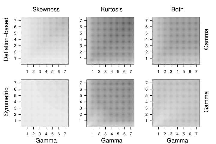
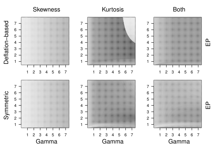
Both discussed projection pursuit methods produce consistent estimates, $\sqrt{n}\ vec(\hat{\textbf{W}}_{1}-\textbf{I}_{d})\rightarrow_{d}N_{d^{2}}(\textbf{0},\boldsymbol{\Phi}_{1})$, and their comparison should thus be made using the asymptotic covariance matrix $\boldsymbol{\Phi}_{1}$. A global measure of variation is given by

where $\sum_{k=1}^{d}ASV(\hat{w}_{kk})$ is the same for both estimates and for all $\alpha$, see Theorems 4.2 and 5.2. Conveniently, for both methods $ASV(\hat{w}_{kl})$, for $k\neq l$, depends only on the distributions of the components $z_{k}$ and $z_{l}$ and is not affected by the dimensions $d$ and $p$. Consequently it is sufficient to consider, as in Miettinen et al. (2015), only the values $V_{12}:=ASV(\hat{w}_{12})+ASV(\hat{w}_{21})$ for different choices of two marginal distributions when measuring their influence to the asymptotic performance. For the symmetric projection pursuit we have $V_{12}=B_{12}+B_{21}$ and, assuming that the component $z_{j}$, $j=1,2$, is extracted first, for the deflation-based projection pursuit we have $V_{12}=2A_{j}+1$.

The two marginal distributions were chosen as standardized versions of either the exponential power distribution, $\mbox{EP}(\lambda)$, or the gamma distribution, $\Gamma(\lambda)$, with the respective densities

with $\tau_{1},\tau_{2}>0$ and a positive shape parameter $\lambda$. The quantity $V_{12}$ depends on the marginal distributions only through their shape parameters $\lambda$, see Miettinen et al. (2015) for more details. For both methods, we distinguished the versions using third cumulants only, $\alpha=1$, fourth cumulants only, $\alpha=0$, and a convex combination with the weight $\alpha=0.8$, see Section 7 for motivating this choice. We then computed the value of $V_{12}$ for different combinations of distribution families and shape parameters using numerical integration and Theorems 4.2 and 5.2 and the results are shown in Figures 3 and 4. Note that we do not report the results in cases where both components come from the symmetric exponential power family as then the asymptotic variances of the estimates with $0<\alpha<1$ are the same as the asymptotic variances of the estimates with $\alpha=0$ (since skewness carries no information, both distributions being symmetric) and the results for $\alpha=0$ are already given in Miettinen et al. (2015). In the figures a darker shade indicates a larger value so that the performance of a particular method is at its best in the areas of lighter color.

From the contour plots it is evident that performance-wise the methods are very close to each other, although, not counting the anomaly in the middle plot of the top row of Figure 4, the symmetric projection pursuit gives in general asymptotically slightly more accurate results. Also, as the distributions in Figure 4 are respectively skewed and symmetric, skewness contains in these settings more information on the separation than kurtosis, explaining why the left-most plots have the overall lightest shade.

Apart from estimating the individual signals, another interesting objective is the estimation of the whole signal subspace. Assuming $\boldsymbol{\Omega}=\textbf{I}_{p}$, we approach the problem via the orthogonal projection matrix

giving an orthogonal projection onto the signal subspace. Our main result is then as follows.

Theorem 6.2 essentially states that the asymptotic behavior of the estimated projection matrix $\hat{\textbf{P}}$ depends only on that of $\hat{\textbf{W}}_{2}$, and not on how well the signals are separated from each other as measured by $\hat{\textbf{W}}_{1}$. Since $\sqrt{n}\ vec(\hat{\textbf{W}}_{2})\rightarrow_{d}N_{(p-d)^{2}}(\textbf{0},\boldsymbol{\Phi}_{2})$, a natural measure for a particular method’s ability to estimate the signal subspace is then

the sum of asymptotic variances of the elements of $\hat{\textbf{W}}_{2}$. Comparison of Figures 1 and 2 now easily yields the conclusion that both discussed projection pursuit methods are asymptotically equally adept at estimating the signal subspace. That is, if we are only interested in separating the signal from the noise, it does not matter asymptotically whether we use the method of Definition 4.1 or 5.1.

We next compare the methods’ performances as the relative amount of noise in the model is increased. Assuming $d<p$, one possible measure for the accuracy of the separation is given by

where $\boldsymbol{\Omega}$ is the true mixing matrix. The measure (5) can be seen as an analogue of the minimum distance index (MDI) (Ilmonen et al., 2010) for non-square matrices and similar techniques as used in proving Theorem 4.1 in Ilmonen et al. (2012) show that $0\leq D(\hat{\textbf{W}})\leq 1$, the value zero indicating perfect separation. Furthermore, the techniques used in Ilmonen et al. (2012) can be used to show that the computation of $D$ can be reduced to an optimization problem over a set of finite support and that the limiting distribution of $ndD^{2}(\hat{\textbf{W}})$ is a weighted sum of independent chi-squared variables with one degree of freedom. The expectation of this limiting distribution is then the sum of the weights, that is, the sum of asymptotic variances of the off-diagonal elements of $\hat{\textbf{W}}$, given by $tr(\boldsymbol{\Phi}_{1})-\sum_{k=1}^{d}ASV(\hat{w}_{kk})+tr(\boldsymbol{\Phi}_{2})$.

For our simulation setting we chose $d=3$, the signal vector s having Uniform$(0,1)$, Exponential$(1)$ and Laplace$(0,1)$ components each standardized to have zero mean and unit variance and the amount of Gaussian noise was taken to be $p-d=0$, $5$, $10$, $20$. Moreover, we considered the sample sizes $n=1000$, $2000$, $4000$, $8000$, $16000$, $32000$ and two different weightings $\alpha=0.2$, $0.8$. The latter of these is motivated in Section 7 and the former can be seen as the “opposite” of that. Due to the affine equivariance of the methods we used, without loss of generality, the mixing matrix $\boldsymbol{\Omega}=\textbf{I}_{p}$. For each of the 2000 repetitions we ran the two projection pursuit algorithms using the alternative gradients in Remark 2.1 with the initial values based on FOBI as discussed in Remarks 4.1 and 5.1 and then computed the corresponding values $D(\hat{\textbf{W}})$.

The averages of $ndD^{2}(\hat{\textbf{W}})$ over the repetitions under the previous combinations of parameters are shown in Figure 5, from which three immediate remarks can be made: the choice $\alpha=0.8$ gives uniformly better results, the symmetric projection pursuit is in all cases slightly superior to the deflation-based one and this difference gets relatively smaller and smaller by increasing the amount of noise. The latter observation is easily explained by noticing that, with respect to the expected value of the limiting distribution of $ndD^{2}(\hat{\textbf{W}})$, the two methods differ only by having different matrices $\boldsymbol{\Phi}_{1}$. As the number of noise is increased the matrix $\boldsymbol{\Phi}_{2}$ common to both methods gets larger while $\boldsymbol{\Phi}_{1}$ retains its size and its relative importance thus diminishes by the addition of noise. As a conclusion, for data with high signal-to-noise ratio (SNR) the use of the symmetric version is advocated and for data with low SNR there is not much difference between the discussed methods.

Given that all the methods allow tuning in the form of the weighting parameter $\alpha$, a natural question is whether there exists some optimal choice of weighting for any particular choice of signal distributions. We approach this question in the context of cluster identification. Both skewness and kurtosis have been used before for similar purposes, see e.g. Jones and Sibson (1987) and Peña and Prieto (2001).

For the model, assume that z is a mixture of two multivariate normal distributions, namely

standardized to have zero mean and identity covariance matrix with $\pi\in(0,1)$, $\mu\in\mathbb{R}\backslash\{0\}$ and $\textbf{e}_{1}=(1,0,\ldots,0)^{T}$. The true dimension is then $d=1$ and $\textbf{s}\in\mathbb{R}$ has a univariate bimodal distribution. Thus all signal separation functionals now consist of only one row. The current setting can also be seen as the problem of estimating the Fisher linear discrimination subspace without knowing the group membership.

A motivation to use both third and fourth cumulants simultaneously in this context stems from the fact that non-trivial normal mixtures of the form (6) can have zero skewness or zero excess kurtosis. Namely, symmetric mixtures, $\pi=0.5$, have zero skewness and mixtures with either $\pi=\pi_{0}:=(3+\sqrt{3})^{-1}$ or $\pi=1-\pi_{0}$ have zero excess kurtosis, see Preston (1953). This means that neither third nor fourth cumulants alone can find the latent groups for all values of $\pi$, a problem not encountered when using any non-trivial convex combination of them.

For $d=1$, the deflation-based and symmetric estimates are the same and the accuracy of the estimation of the signal is provided by $A_{1}$, see Theorems 4.2 and 5.2. We searched the values of $\alpha$ minimizing $A_{1}$ for $\pi\in(0,1)$ and the three choices of $\mu=2,5,10$ and the results are shown in Figure 6 (we only need to consider the interval $\pi\in(0,0.5]$ due to symmetry). First, the plot shows that the choice of $\mu$ has hardly any effect on the optimal value of $\alpha$. Secondly, we see the two discontinuity points discussed previously, $\pi=\pi_{0}$ and $\pi=0.5$. And thirdly, we observe that the curve goes to zero when approaching the point $\pi_{0}$ from the right. This counterintuitively suggests using only fourth cumulants even though $\kappa_{1}\approx 0$ in the vicinity of $\pi_{0}$. However, a careful examination shows that when $\pi=\pi_{0}+\epsilon$ for some small $\epsilon>0$, the quantity $A_{1}$ as a function of $\alpha$ indeed has a global minimum near zero but it also satisfies $\text{lim}_{\alpha\rightarrow 0+}A_{1}(\alpha)=\infty$. Thus for practical purposes the global minimum is too close to zero to be of any use.

References

- Amari et al. (1996) Amari, S.-I., A. Cichocki, and H. H. Yang (1996). A new learning algorithm for blind signal separation. Advances in neural information processing systems, 757–763.
- Blanchard et al. (2005) Blanchard, G., M. Sugiyama, M. Kawanabe, V. Spokoiny, and K.-R. Müller (2005). Non-Gaussian component analysis: a semi-parametric framework for linear dimension reduction. In Advances in Neural Information Processing Systems, pp. 131–138.
- Bonhomme and Robin (2009) Bonhomme, S. and J.-M. Robin (2009). Consistent noisy independent component analysis. Journal of Econometrics 149(1), 12 – 25.
- Brys et al. (2005) Brys, G., M. Hubert, and P. Rousseeuw (2005). A robustification of independent component analysis. Journal of Chemometrics 19(5), 364–375.
- Cardoso (1989) Cardoso, J.-F. (1989). Source separation using higher order moments. In International Conference on Acoustics, Speech, and Signal Processing, 1989. ICASSP-89., pp. 2109–2112. IEEE.
- Cardoso and Souloumiac (1993) Cardoso, J.-F. and A. Souloumiac (1993). Blind beamforming for non-Gaussian signals. In IEE Proceedings F (Radar and Signal Processing), Volume 140, pp. 362–370. IET.
- Chen and Bickel (2006) Chen, A. and P. Bickel (2006). Efficient independent component analysis. Annals of Statistics 34, 2825–2855.
- Comon (1994) Comon, P. (1994). Independent component analysis, a new concept? Signal processing 36(3), 287–314.
- Comon and Jutten (2010) Comon, P. and C. Jutten (2010). Handbook of Blind Source Separation: Independent component analysis and applications. Academic press.
- Comon et al. (2015) Comon, P., Y. Qi, and K. Usevich (2015). A polynomial formulation for joint decomposition of symmetric tensors of different orders. In Latent Variable Analysis and Signal Separation, pp. 22–30. Springer.
- Comon and Rajih (2006) Comon, P. and M. Rajih (2006). Blind identification of under-determined mixtures based on the characteristic function. Signal Processing 86(9), 2271–2281.
- Eddelbuettel and François (2011) Eddelbuettel, D. and R. François (2011). Rcpp: Seamless R and C++ integration. Journal of Statistical Software 40(8), 1–18.
- Eddelbuettel and Sanderson (2014) Eddelbuettel, D. and C. Sanderson (2014, March). RcppArmadillo: Accelerating R with high-performance C++ linear algebra. Computational Statistics and Data Analysis 71, 1054–1063.
- Friedman and Tukey (1974) Friedman, J. and J. Tukey (1974, Sept). A projection pursuit algorithm for exploratory data analysis. IEEE Transactions on Computers C-23(9), 881–890.
- Hallin and Mehta (2015) Hallin, M. and C. Mehta (2015). R-estimation for asymmetric independent component analysis. Journal of the American Statistical Association 110, 218–232.
- Hastie and Tibshirani (2003) Hastie, T. and R. Tibshirani (2003). Independent component analysis through product density estimation. In S. Becker and K. Obermayer (Eds.), Advances in Neural Information Processing Systems, Volume 15, pp. 665–672. Cambridge, MA: MIT Press.
- Hornik (2016) Hornik, K. (2016). clue: Cluster ensembles. R package version 0.3-51.
- Huber (1985) Huber, P. J. (1985). Projection pursuit. The Annals of Statistics 13(2), 435–475.
- Hyvärinen (1999) Hyvärinen, A. (1999). Fast and robust fixed-point algorithms for independent component analysis. Neural Networks, IEEE Transactions on 10(3), 626–634.
- Hyvärinen and Oja (1997) Hyvärinen, A. and E. Oja (1997). A fast fixed-point algorithm for independent component analyis. Neural Computation 9, 1483–1492.
- Ibragimov (2014) Ibragimov, I. (2014). On the Ghurye–Olkin–Zinger theorem. Journal of Mathematical Sciences 199(2), 174–183.
- Ilmonen et al. (2010) Ilmonen, P., K. Nordhausen, H. Oja, and E. Ollila (2010). A new performance index for ICA: properties, computation and asymptotic analysis. In Latent Variable Analysis and Signal Separation, pp. 229–236. Springer.
- Ilmonen et al. (2012) Ilmonen, P., K. Nordhausen, H. Oja, and E. Ollila (2012). On asymptotics of ICA estimators and their performance indices. arXiv preprint arXiv:1212.3953.
- Ilmonen et al. (2012) Ilmonen, P., H. Oja, and R. Serfling (2012). On invariant coordinate system (ICS) functionals. International Statistical Review 80(1), 93–110.
- Ilmonen and Paindaveine (2011) Ilmonen, P. and D. Paindaveine (2011). Semiparametrically efficient inference based on signed ranks in symmetric independent components models. Annals of Statistics 39, 2448–2476.
- Jarque and Bera (1987) Jarque, C. M. and A. K. Bera (1987). A test for normality of observations and regression residuals. International Statistical Review/Revue Internationale de Statistique, 163–172.
- Jones and Sibson (1987) Jones, M. C. and R. Sibson (1987). What is projection pursuit? Journal of the Royal Statistical Society. Series A (General), 1–37.
- Karvanen et al. (2002) Karvanen, J., J. Eriksson, and V. Koivunen (2002). Adaptive score functions for maximum likelihood ICA. Journal of VLSI signal processing systems for signal, image and video technology 32(1-2), 83–92.
- Karvanen and Koivunen (2002) Karvanen, J. and V. Koivunen (2002). Blind separation methods based on Pearson system and its extensions. Signal Processing 82(4), 663 – 673.
- Karvanen and Koivunen (2004) Karvanen, J. and V. Koivunen (2004). Independent component analysis via optimum combining of kurtosis and skewness-based criteria. Journal of the Franklin Institute 341(5), 401–418.
- Kawanabe (2005) Kawanabe, M. (2005). Linear dimension reduction based on the fourth-order cumulant tensor. In Artificial Neural Networks: Formal Models and Their Applications–ICANN 2005, pp. 151–156. Springer.
- Li et al. (2011) Li, X.-L., T. Adalı, and M. Anderson (2011). Joint blind source separation by generalized joint diagonalization of cumulant matrices. Signal Processing 91(10), 2314–2322.
- Matteson and Tsay (2016) Matteson, D. S. and R. S. Tsay (2016). Independent component analysis via distance covariance. Journal of the American Statistical Association 0(ja), 1–38.
- Miettinen et al. (2013) Miettinen, J., K. Nordhausen, H. Oja, and S. Taskinen (2013, May). Fast equivariant JADE. In IEEE International Conference on Acoustics, Speech and Signal Processing (ICASSP) 2013, pp. 6153–6157.
- Miettinen et al. (2014) Miettinen, J., K. Nordhausen, H. Oja, and S. Taskinen (2014). Deflation-based FastICA with adaptive choices of nonlinearities. IEEE Transactions on Signal Processing 62(21), 5716–5724.
- Miettinen et al. (2017) Miettinen, J., K. Nordhausen, H. Oja, S. Taskinen, and J. Virta (2017). The squared symmetric FastICA estimator. Signal Processing 131, 402 – 411.
- Miettinen et al. (2015) Miettinen, J., S. Taskinen, K. Nordhausen, and H. Oja (2015). Fourth moments and independent component analysis. Statistical Science 30, 372–390.
- Moreau (2001) Moreau, E. (2001). A generalization of joint-diagonalization criteria for source separation. IEEE Transactions on Signal Processing 49(3), 530–541.
- Nordhausen et al. (2015) Nordhausen, K., J.-F. Cardoso, J. Miettinen, H. Oja, E. Ollila, and S. Taskinen (2015). JADE: Blind Source Separation Methods Based on Joint Diagonalization and Some BSS Performance Criteria. R package version 1.9-93.
- Nordhausen et al. (2011) Nordhausen, K., P. Ilmonen, A. Mandal, H. Oja, and E. Ollila (2011). Deflation-based FastICA reloaded. In Proceedings of 19th European Signal Processing Conference, pp. 1854–1858.
- Nordhausen et al. (2008) Nordhausen, K., H. Oja, and E. Ollila (2008). Robust independent component analysis based on two scatter matrices. Austrian Journal of Statistics 37(1), 91–100.
- Nordhausen et al. (2008) Nordhausen, K., H. Oja, and D. E. Tyler (2008). Tools for exploring multivariate data: The package ICS. Journal of Statistical Software 28(6), 1–31.
- Ollila (2010) Ollila, E. (2010). The deflation-based FastICA estimator: Statistical analysis revisited. IEEE Transactions on Signal Processing 58(3), 1527–1541.
- Peña and Prieto (2001) Peña, D. and F. J. Prieto (2001). Cluster identification using projections. Journal of the American Statistical Association 96(456).
- Preston (1953) Preston, E. J. (1953). A graphical method for the analysis of statistical distributions into two normal components. Biometrika 40(3-4), 460–464.
- R Core Team (2015) R Core Team (2015). R: A Language and Environment for Statistical Computing. Vienna, Austria: R Foundation for Statistical Computing.
- Risk et al. (2015) Risk, B. B., D. S. Matteson, and D. Ruppert (2015). Likelihood component analysis. arXiv:1511.01609 [stat.ME].
- Samworth and Yuan (2012) Samworth, R. J. and M. Yuan (2012). Independent component analysis via nonparametric maximum likelihood estimation. The Annals of Statistics 40(6), 2973–3002.
- Theis et al. (2011) Theis, F. J., M. Kawanabe, and K.-R. Muller (2011). Uniqueness of non-Gaussianity-based dimension reduction. IEEE Transactions on Signal Processing 59(9), 4478–4482.
- Tyler et al. (2009) Tyler, D., Critchley, F., L. Dümbgen, and H. Oja (2009). Invariant coordinate selection. Journal of Royal Statistical Society, Series B 71, 549–592.
- Virta et al. (2015) Virta, J., K. Nordhausen, and H. Oja (2015). Joint use of third and fourth cumulants in independent component analysis. arXiv preprint arXiv:1505.02613.
- Wei (2015) Wei, T. (2015). A convergence and asymptotic analysis of the generalized symmetric FastICA algorithm. IEEE Transactions on Signal Processing 63(24), 6445–6458.
- Wickham (2009) Wickham, H. (2009). ggplot2: Elegant Graphics for Data Analysis. Springer-Verlag New York.
- Woods et al. (2015) Woods, R. P., L. K. Hansen, and S. Strother (2015, 03). How many separable sources? Model selection in independent components analysis. PLoS ONE 10(3), 1–39.