Transport signatures of Kondo physics and quantum criticality in graphene with magnetic impurities.

Graphene is a two–dimensional carbon allotrope characterized by low energy excitations that behave like two–dimensional, massless Dirac fermions.[1] Many desirable electronic properties have been predicted for graphene as a result of the chiral nature of its charge carriers,[2] making it an ideal platform for the fabrication of novel devices. These properties, along with its outstanding mechanical characteristics, have earned graphene a place in contemporary popular culture as the “material of the future.”

Combining graphene’s electronic properties with magnetism has become a major driving force for research on this material in recent years. Although ferromagnetic order is suppressed in pristine bulk samples,[3] there are a number of ways to induce magnetic moments in graphene, ranging from adsorption of magnetic [4, 5, 6] and non–magnetic [7, 8] atoms to proposals for vacancy–induced $\pi$-magnetism.[9, 10, 11, 12, 13, 14]

Once magnetic moments are present in the graphene lattice, fascinating many–body effects can be expected. The coupling of a localized magnetic moment and the (real) spin of Dirac electrons in neutral graphene has long been theorized as a realization of the linear pseudogap Kondo model,[15, 16] where a magnetic impurity couples to a fermionic density of states that vanishes linearly at the Fermi energy. One of the main features of this type of system is a quantum phase transition from a local–moment phase to a Kondo phase, where the atom’s magnetic moment becomes screened by itinerant electrons. [15, 16, 17, 18, 19]

Experimental evidence for the Kondo effect has emerged recently in a graphene system with atomic vacancies.[10] A most intriguing feature of those experiments is an observed temperature dependence of the resistivity that is compatible with the metallic Kondo effect for a vast range of gate voltages, including at the charge neutrality point. This leads us to two questions: Why are no pseudogap effects observed? And, what would the transport signatures of impurity quantum criticality be? One possible answer to the first question is that sample disorder may play an important role[20] in masking the pseudogap signatures. Another possibility is that in the experiments the samples are only probed effectively away from charge neutrality, where metallic Kondo behavior predominates.[21, 22, 23]

In this paper we address the second question by calculating the impurity contribution to the linear resistivity of a graphene sample. In a recent work[24] we calculated the transport properties of graphene in the presence of a dilute ensemble of non–magnetic impurities, and found that impurity symmetry plays a determinant role in the system transport properties. Here we turn our attention to magnetic impurities, such as transition–metal[4, 5, 6] and hydrogen[7, 8] adatoms, and both symmetric and reconstructed vacancies.[25, 26, 27, 28]

Using numerical renormalization–group (NRG) calculations we found that the interplay between symmetry and strong correlations leads to a rich phenomenology, including an impurity–dependent quantum phase transition (QPT) in charge neutrality related to the pseudogap Anderson model, and the emergence of Kondo physics when a back gate is applied. For top–site adsorbates and reconstructed vacancies lacking $C_{3v}$ and inversion symmetry, both regimes produce experimentally accessible signatures in the bulk resistivity profile: the QPT is signaled by a power–law divergence of the resistivity at low temperatures, when the energy of the impurity level crosses a critical value. Surprisingly, this behavior is qualitatively similar to that of the non–interacting case,[24] with the main effect of interactions being a renormalization of the critical point parameters. By contrast, the presence of a back gate driving the system away from charge neutrality leads to screening of the impurity spin through Kondo correlations, signaled by a zero–energy peak in the impurity density of states and a low–temperature plateau of enhanced resistivity.

In the case of highly symmetric magnetic impurities, such as unreconstructed vacancies ($C_{3v}$) and hollow–site adsorbates ($C_{3v}$ and inversion), quantum criticality is also observed in neutral graphene, described by the cubic pseudogap Anderson model. Furthermore, these impurities display robust Kondo physics for sensible values of the carrier density, with Kondo temperatures comparable to those obtained for their less symmetric counterparts. Interestingly, we find that such impurities do not contribute to the sample resistivity, a result we had previously obtained in the non–interacting case.[24, 29] As a consequence, they are not easily captured in bulk transport measurements and need to be probed locally.

The remainder of this article is organized as follows: In Sec. II we introduce low–energy Hamiltonians for graphene coupled to four different impurity types. These models are studied in Sec. III using NRG calculations. We begin by describing the single–impurity ground state for different model parameters in Sections III.1 and III.2, where we discuss an impurity–dependent QPT in charge neutrality and the onset of Kondo correlations when a back gate is applied. Then, in Sec. III.3 we evaluate the impurity contribution to the resistivity as a function of temperature and chemical potential, in graphene samples with mixtures of symmetric and non–symmetric adatoms or vacancies. Our conclusions are presented in Sec. IV.

A single magnetic impurity in a graphene sample can be modeled by the Anderson–type Hamiltonian $H=H_{\mathrm{I}}+H_{\mathrm{G}}+H_{\text{I-G}}$, where $H_{\mathrm{I}}$ represents the impurity, $H_{\mathrm{G}}$ the graphene sheet, and $H_{\text{I-G}}$ is a hybridization term. The interacting impurity Hamiltonian is

where ($\varepsilon_{I}-\mu$) is the impurity orbital energy measured with respect to the graphene chemical potential, $U$ is the electrostatic energy cost of double occupancy, the operators $d_{I,s}^{\dagger}$ ($d_{I,s}$) create (annihilate) electrons of spin projection $s$ in the impurity orbital, and $n_{I,s}=d_{I,s}^{\dagger}d_{I,s}$ are the corresponding number operators. The graphene sample can be described by the Hamiltonian

with $\psi_{s}(\boldsymbol{\mathbf{k}})=(a_{s}(\boldsymbol{\mathbf{k}}),\,b_{s}(\boldsymbol{\mathbf{k}}))^{T}$, $a_{s}(\boldsymbol{\mathbf{k}})$ [$b_{s}(\boldsymbol{\mathbf{k}})$] the annihilation operator for sublattice $A$ ($B$) electrons, and

$a\approx 1.42\,\mathrm{\r{A}}$ is the honeycomb lattice constant, $t$ the nearest–neighbor hopping energy, and $\hat{\mathbf{u}}_{1}=\hat{\mathbf{x}}$, $\hat{\mathbf{u}}_{2}=-\hat{\mathbf{x}}/2+\hat{\mathbf{y}}\sqrt{3}/2$ and $\hat{\mathbf{u}}_{3}=-\hat{\mathbf{x}}/2-\hat{\mathbf{y}}\sqrt{3}/2$ are nearest–neighbor vectors. Diagonalizing $H_{\mathrm{G}}$ gives two energy bands with dispersions $\epsilon_{\pm}(\boldsymbol{\mathbf{k}})=\pm t|\Phi(\boldsymbol{\mathbf{k}})|$ and corresponding operators $c_{s}(\boldsymbol{\mathbf{k}})=(c_{+,s}(\boldsymbol{\mathbf{k}}),\,c_{-,s}(\boldsymbol{\mathbf{k}}))^{T}$. These are related to the $\psi$-basis operators as $\psi_{s}(\boldsymbol{\mathbf{k}})=U_{\boldsymbol{\mathbf{k}}}c_{s}(\boldsymbol{\mathbf{k}})$, with the similarity transformation

In its general form, the hybridization term $H_{\text{I-G}}$ couples the impurity to the graphene momentum state $\boldsymbol{\mathbf{k}}$ in subband $\alpha$ as

with $V$ a real hopping constant. Encoded in $\Theta_{I}^{\alpha}(\boldsymbol{\mathbf{k}})$ are the symmetry properties of the impurity orbital. In this article we study four of the most common atomic impurities found in real graphene samples: top–site ($\mathrm{TOP}$) and hollow–site ($\mathrm{HS}$) adatoms, and symmetric ($\mathrm{VAC}$) and reconstructed ($\mathrm{REC}$) single vacancies. Their corresponding couplings $\Theta_{I}^{\alpha}(\boldsymbol{\mathbf{k}})$ are evaluated in Appendix A using the real–space form of the graphene Hamiltonian, and their symmetry properties are discussed below.

$\mathrm{TOP}$ adatoms are the simplest of these impurity types. They sit on top of and couple exclusively to a single carbon atom [Fig. 1(a)], thus singling out one of the sublattices and locally breaking inversion symmetry. Their point–like isotropic nature makes $\mathrm{TOP}$ adatoms couple equally to all graphene momenta as

Examples of $\mathrm{TOP}$ impurities have been recently reported in experiments with hydrogen atoms chemisorbed onto graphene.[30, 8] Although the impurity states were found to extend over several lattice constants from the adsorption site, local breaking of inversion symmetry was observed, and the model (6) may be used as a first approximation.

On the other hand, more usual magnetic impurity candidates, such as transition metals, tend to adsorb in the hollow site.[4, 5, 6] $\mathrm{HS}$ adatoms with $s$ or $d_{z^{2}}$ valence orbitals will couple equally to both sublattices, and thus preserve both the inversion and point symmetries [Fig. 1(b)]. The resulting coupling functions

vanish at the $K$ and $K^{\prime}$ points, and possess $C_{3v}$ symmetry about those point inherited from the function $\Phi(\boldsymbol{\mathbf{k}})$, as shown in Figs. 2(c) and 2(d). Moreover, inversion symmetry guarantees the presence of “nodes” in the coupling function—branches of graphene momenta that remain decoupled from the impurity degrees of freedom.[24] As we will discuss in Sec. III.3, the zeros of the coupling function play a determinant role in the impurity contribution to the system transport properties.

Vacancies introduce localized midgap states in graphene[31, 32, 33, 34] that can develop magnetic moments[26, 20, 27] as a result of Coulomb charging–energy effects.[35] In fact, recent studies show that such charging energies can be large[27] (of order $0.5\,\mathrm{eV}$), leading to the formation of effective $\pi$-like magnetic moments. In the case of symmetric vacancies, experiments have demonstrated charge accumulation at the vacancy site,[36] constituting the type of impurity we label as $\mathrm{VAC}$. To a first approximation, this impurity will couple identically and exclusively to its three nearest neighbors, belonging to the opposite sublattice[37] [Fig. 1(c)]. As a result, a $\mathrm{VAC}$ impurity will possess $C_{3v}$ symmetry but break local inversion symmetry. This is encoded in the coupling

which is $C_{3v}$-symmetric about, and vanishes at the $K$ and $K^{\prime}$ points [Fig. 2(a)], but lacks the inversion–symmetry nodes displayed by $\mathrm{HS}$ impurities.

Finally, vacancies with bond reconstruction[38, 39, 40] are the least symmetric of all cases, breaking both $C_{3v}$ and inversion symmetries. Bond reconstruction consists of a local deformation due to Jahn-Teller effects,[38, 22, 41, 42, 43, 44] which allows a coupling between one carbon’s $sp^{2}$ orbital and the $\pi$ orbitals belonging to the other two carbons surrounding the vacancy site—what we call the $\mathrm{REC}$ impurity [Fig. 1(d)]. Placing the impurity orbital explicitly at $a\hat{\boldsymbol{\mathbf{u}}}_{j}$ from the vacancy center, the coupling is given by

Anticipating our transport discussion, one may conclude that such breaking of rotational symmetry should introduce dramatic anisotropy in the resistivity tensor $\varrho^{ij}$. In an ensemble, however, the $\mathrm{REC}$ impurities will occur at $j=1,\,2$ and $3$ with equal probability. In the dilute limit, where second and higher–order coherent scattering processes are neglected, the $\mathrm{REC}$ impurity distribution can be represented by the average scattering rate

Eq. (10) shows that the spatial averaging recovers $C_{3v}$ symmetry, but destroys the quantum interference leading to the zeros at $K$ and $K^{\prime}$ [Fig. 2(b)].

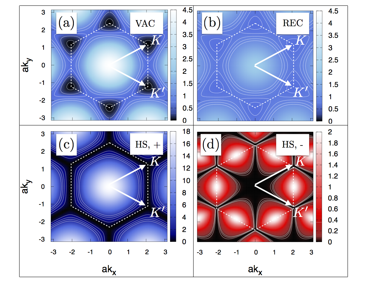
At low energies the graphene sample properties depend only on the momentum states $\boldsymbol{\mathbf{\kappa}}$ close to the Dirac points ($\kappa\ll K$). The low–energy theory is obtained by making

and $h(\boldsymbol{\mathbf{k}})\rightarrow\hbar v_{F}\,\tau^{3}\boldsymbol{\mathbf{\sigma}}\cdot\boldsymbol{\mathbf{\kappa}}$, where $\hbar v_{F}=3at/2$, $\tau^{3}$ is the third Pauli matrix in valley space, and $\boldsymbol{\mathbf{\sigma}}$ is the vector of Pauli matrices in sublattice space. Naturally, this model produces four bands $\epsilon_{1}(\kappa)=\epsilon_{4}(\kappa)=-\epsilon_{2}(\kappa)=-\epsilon_{3}(\kappa)=\hbar v_{F}\kappa$, corresponding to the valence and conduction Dirac cones at the $K$ and $K^{\prime}$ points.

In this approximation the influence of graphene electrons with energy $\omega$ on the impurity is determined by the hybridization function

where $\kappa_{c}=3^{-3/4}(8\pi)^{1/2}a^{-1}$ is the Debye momentum cutoff,[2] and $\Theta_{I}^{\mu}(\boldsymbol{\mathbf{\kappa}})$ are the elements of the $4\times 1$ coupling matrix

The hybridization functions corresponding to the couplings (6) through (9) are

where $\Gamma_{0}=2\pi V^{2}/D$, and $D=\hbar v_{F}\kappa_{c}$ is the half–bandwidth of the graphene dispersion. Notice that the four impurity types can be grouped into two categories, depending on the low–energy behavior of their hybridization functions: the non-symmetric $\mathrm{TOP}$ and $\mathrm{REC}$ impurities, which couple to low–energy graphene states as $|\omega|$, and the highly–symmetric $\mathrm{HS}$ and $\mathrm{VAC}$ impurities, which do so as $|\omega|^{3}$, a result previously obtained in Ref. [19]. For simplicity, in the following sections we will explicitly discuss $\mathrm{TOP}$ and $\mathrm{HS}$ impurities as representatives of their corresponding categories, with the express understanding that $\mathrm{REC}$ and $\mathrm{VAC}$ impurities, respectively, display qualitatively similar behaviors.

For $U\neq 0$ the Hamiltonian $H$ describes a system with strong spin correlations between the impurity and the graphene band. In the specific case of charge neutrality ($\mu\!=\!0$), it corresponds to the pseudogap Anderson model,[16] where the effective density of states coupled to the impurity level vanishes at the Fermi level as a power law $|\omega/D|^{r}$. Eqs. (14) give $r\!=\!1$ for $\mathrm{TOP}$ and $\mathrm{REC}$ impurities and $r\!=\!3$ for $\mathrm{HS}$ and $\mathrm{VAC}$ impurities.

In general, this problem cannot be solved analytically in closed form. Instead, we used Wilson’s numerical renormalization group (NRG),[45, 46, 47, 48] adapted for a generic density of states following Ref. [16]. NRG is generally regarded as the method of choice for studying strongly correlated quantum impurity problems. It consists of numerically diagonalizing the Hamiltonian $H$ by logarithmically discretizing the energy–dependent hybridization functions [Eqs. (14)] into energy bins $D\Lambda^{-(n+1)}<\pm\omega_{\pm,n}<D\Lambda^{-n}$, with $\Lambda>1$ the discretization parameter and $n\geq 0$ an integer. This discretization scheme prevents artificially introducing an energy scale into the problem that may obscure any emergent scales, such as the Kondo temperature. The states belonging to bins $(\pm,n)$ are mapped onto a chain of fermionic states with local energies and hopping terms of order $D\Lambda^{-n/2}$ that fall exponentially with $n$. This so–called Wilson chain is coupled to the impurity site ($n\!=\!-1$) and diagonalized iteratively, deriving at every iteration $n$ an effective free energy valid for temperatures of order $D\Lambda^{-n/2}$.

In the following sections we present NRG results for the spectral density and thermodynamic properties of the different impurity types. The temperature–dependent charge and magnetic susceptibility will be used to accurately characterize the system ground state, unveiling a quantum phase transition (QPT) as a function of the impurity energy $\varepsilon_{I}$ in the absence of a back gate ($\mu=0$), and the screening of the impurity spin through Kondo correlations for $\mu\!\neq\!0$. The impurity spectral density will be used to determine the low–temperature electronic transport properties of the graphene sample based on the formalism presented in Ref. [24]. All calculations shown below were carried out with discretization factor $\Lambda=2.5$, retaining approximately $1024$ states after each iteration. The spectral densities presented in Sec. III.2 were evaluated using the density–matrix NRG method (DM-NRG).[49]

We have studied the thermodynamic, spectral and linear transport signatures of dilute magnetic vacancies and adatoms in mesoscopic graphene. Our numerical results indicate that the quantum–critical[17, 51, 52] behavior of magnetic impurities in neutral graphene is in direct correspondence with the single–particle picture of nonmagnetic impurities. Local interactions produce a level shift $|\varepsilon_{I}^{*}|$, corresponding to the critical level energy, and renormalize the impurity-graphene hybridization. Quantum criticality is analogous to bound–state formation by resonant scatterers,[24] and in the case of top adsorbates and reconstructed vacancies introduces a sharp peak in the local density of states that scales with energy as $|\omega|^{-1}$. However, no Kondo physics is observed in the absence of a back gate,[16] and the zero–energy resonance at criticality produces $\sim D^{2}T^{-2}$ resistivity scaling, leading to full insulating behavior at zero temperature, in stark contrast to the well–known Kondo resistivity plateau.

Away from charge neutrality, the system enters a Kondo phase that strongly depends on the impurity symmetry: While asymmetric impurities, such as top–adsorbates and reconstructed vacancies, remain in the Kondo phase for a wide range of back gate voltages, symmetric vacancies and hollow–site adsorbates exhibit Kondo correlations only within parameter–dependent limits. Nonetheless, symmetric and non–symmetric impurities display comparable, and experimentally accessible Kondo temperatures ranging from order $1\,\mathrm{K}$ to order $10\,\mathrm{K}$ for realistic parameters,[66, 33] defying earlier expectations.[19, 23]

As in the case of nonmagnetic (noninteracting) impurities, symmetry is critical to the system electronic transport. Unreconstructed vacancies and other $C_{3v}$–symmetric impurities remain decoupled from graphene states at the $K$ and $K^{\prime}$ points, which in charge neutrality remain available for electrons to move coherently through the sample. In the presence of a back gate, however, our results indicate that symmetric vacancies will contribute strongly to the resistivity through Kondo scattering. In contrast, inversion–symmetric impurities, such as hollow–site adsorbates, are decoupled from entire momentum branches across the Brillouin zone, and thus never contribute to the resistivity. Although this means that symmetric impurities cannot be probed in the bulk through resistivity measurements,[29] their remarkable properties in criticality and in the Kondo regime can be measured by means of local methods, such as scanning tunneling microscopy (STM).[67]

References

- [1] G. W. Semenoff, Phys. Rev. Lett. 53, 2449 (1984).
- [2] A. H. Castro Neto, F. Guinea, N. M. R. Peres, K. S. Novoselov, and A. K. Geim, Rev. Mod. Phys. 81, 109 (2009).
- [3] N. M. R. Peres, F. Guinea, and A. H. Castro Neto, Phys. Rev. B 72, 174406 (2005).
- [4] T. Eelbo, M. Waśniowska, P. Thakur, M. Gyamfi, B. Sachs, T. O. Wehling, S. Forti, U. Starke, C. Tieg, A. I. Lichtenstein, and R. Wiesendanger, Phys. Rev. Lett. 110, 136804 (2013).
- [5] F. Donati, Q. Dubout, G. Autès, F. Patthey, F. Calleja, P. Gambardella, O. V. Yazyev, and H. Brune, Phys. Rev. Lett. 111, 236801 (2013).
- [6] F. Donati, L. Gragnaniello, A. Cavallin, F. D. Natterer, Q. Dubout, M. Pivetta, F. Patthey, J. Dreiser, C. Piamonteze, S. Rusponi, and H. Brune, Phys. Rev. Lett. 113, 177201 (2014).
- [7] K. M. McCreary, A. G. Swartz, W. Han, J. Fabian, and R. K. Kawakami, Phys. Rev. Lett. 109, 186604 (2012).
- [8] H. Gonzalez-Herrero, J. M. Gomez-Rodriguez, P. Mallet, M. Moaied, J. J. Palacios, C. Salgado, M. M. Ugeda, J.-Y. Veuillen, F. Yndurain, and I. Brihuega, Science 352, 437 (2016).
- [9] O. V. Yazyev, Rep. Prog. Phys. 73, 56501 (2010).
- [10] J.-H. Chen, L. Li, W. G. Cullen, E. D. Williams, and M. S. Fuhrer, Nature Phys. 7, 535 (2011).
- [11] R. R. Nair, M. Sepioni, I.-L. Tsai, O. Lehtinen, J. Keinonen, A. V. Krasheninnikov, T. Thomson, A. K. Geim, and I. V. Grigorieva, Nat. Phys. 8, 199 (2012).
- [12] R. R. Nair, I.-L. Tsai, M. Sepioni, O. Lehtinen, J. Keinonen, A. V. Krasheninnikov, A. H. Castro Neto, M. I. Katsnelson, a. K. Geim, and I. V. Grigorieva, Nat. Commun. 4, 2010 (2013).
- [13] S. Just, S. Zimmermann, V. Kataev, B. Büchner, M. Pratzer, and M. Morgenstern, Phys. Rev. B 90, 125449 (2014).
- [14] Y. Zhang, S.-Y. Li, H. Huang, W.-T. Li, J.-B. Qiao, W.-X. Wang, L.-J. Yin, K.-K. Bai, W. Duan, and L. He, Phys. Rev. Lett. 117, 166801 (2016).
- [15] D. Withoff and E. Fradkin, Phys. Rev. Lett. 64, 1835 (1990).
- [16] C. Gonzalez-Buxton and K. Ingersent, Phys. Rev. B 57, 14254 (1998).
- [17] L. Fritz and M. Vojta, Reports on Progress in Physics 76, 032501 (2013).
- [18] M. Vojta, L. Fritz, and R. Bulla, EPL 90, 27006 (2010).
- [19] B. Uchoa, T. G. Rappoport, and A. H. Castro Neto, Phys. Rev. Lett. 106, 016801 (2011).
- [20] V. G. Miranda, L. G. G. V. Dias da Silva, and C. H. Lewenkopf, Phys. Rev. B 90, 201101 (2014).
- [21] P. S. Cornaglia, G. Usaj, and C. A. Balseiro, Phys. Rev. Lett. 102, 046801 (2009).
- [22] T. Kanao, H. Matsuura, and M. Ogata, Journal of the Physical Society of Japan 81, 063709 (2012), http://dx.doi.org/10.1143/JPSJ.81.063709 .
- [23] P.-W. Lo, G.-Y. Guo, and F. B. Anders, Phys. Rev. B 89, 195424 (2014).
- [24] D. A. Ruiz-Tijerina and L. G. G. V. Dias da Silva, Phys. Rev. B 94, 085425 (2016).
- [25] O. V. Yazyev and L. Helm, Phys. Rev. B 75, 125408 (2007).
- [26] M. A. Cazalilla, A. Iucci, F. Guinea, and A. H. Castro Neto, (2012), arXiv:1207.3135 [cond-mat.str-el] .
- [27] V. G. Miranda, L. G. G. V. Dias da Silva, and C. H. Lewenkopf, Phys. Rev. B 94, 075114 (2016).
- [28] L. Rodrigo, P. Pou, and R. Pérez, Carbon 103, 200 (2016).
- [29] J. Duffy, J. Lawlor, C. Lewenkopf, and M. S. Ferreira, Phys. Rev. B 94, 045417 (2016).
- [30] C. Lin, Y. Feng, Y. Xiao, M. Dürr, X. Huang, X. Xu, R. Zhao, E. Wang, X.-Z. Li, and Z. Hu, Nano Letters 15, 903 (2015), pMID: 25621539, http://dx.doi.org/10.1021/nl503635x .
- [31] V. M. Pereira, F. Guinea, J. M. B. Lopes dos Santos, N. M. R. Peres, and A. H. Castro Neto, Phys. Rev. Lett. 96, 036801 (2006).
- [32] V. M. Pereira, J. M. B. Lopes dos Santos, and A. H. Castro Neto, Phys. Rev. B 77, 115109 (2008).
- [33] S. Yuan, H. De Raedt, and M. I. Katsnelson, Phys. Rev. B 82, 115448 (2010).
- [34] O. Lehtinen, J. Kotakoski, A. V. Krasheninnikov, A. Tolvanen, K. Nordlund, and J. Keinonen, Phys. Rev. B 81, 153401 (2010).
- [35] V. M. Pereira, J. Nilsson, and A. H. Castro Neto, Phys. Rev. Lett. 99, 166802 (2007).
- [36] J. Mao, Y. Jiang, D. Moldovan, G. Li, K. Watanabe, T. Taniguchi, M. R. Masir, F. M. Peeters, and E. Y. Andrei, Nat Phys 12, 545 (2016).
- [37] F. Ducastelle, Phys. Rev. B 88, 075413 (2013).
- [38] A. A. El-Barbary, R. H. Telling, C. P. Ewels, M. I. Heggie, and P. R. Briddon, Phys. Rev. B 68, 144107 (2003).
- [39] Y. Ma, P. O. Lehtinen, A. S. Foster, and R. M. Nieminen, New Journal of Physics 6, 68 (2004).
- [40] S. T. Skowron, I. V. Lebedeva, A. M. Popov, and E. Bichoutskaia, Chem. Soc. Rev. 44, 3143 (2015).
- [41] J. J. Palacios and F. Ynduráin, Phys. Rev. B 85, 245443 (2012).
- [42] C.-C. Lee, Y. Yamada-Takamura, and T. Ozaki, Phys. Rev. B 90, 014401 (2014).
- [43] H. Padmanabhan and B. R. K. Nanda, Phys. Rev. B 93, 165403 (2016).
- [44] A. M. Valencia and M. J. Caldas, (2016), arXiv:1611.08246 [cond-mat.mes-hall] .
- [45] K. G. Wilson, Rev. Mod. Phys. 47, 773 (1975).
- [46] H. R. Krishna-murthy, J. W. Wilkins, and K. G. Wilson, Phys. Rev. B 21, 1003 (1980a).
- [47] H. R. Krishna-murthy, J. W. Wilkins, and K. G. Wilson, Phys. Rev. B 21, 1044 (1980b).
- [48] R. Bulla, T. A. Costi, and T. Pruschke, Rev. Mod. Phys. 80, 395 (2008).
- [49] W. Hofstetter, Phys. Rev. Lett. 85, 1508 (2000).
- [50] In dimensionless form, , with the contribution of impurity to the magnetic susceptibility, the Bohr magneton, and the factor.
- [51] M. Vojta and L. Fritz, Phys. Rev. B 70, 094502 (2004).
- [52] L. Fritz and M. Vojta, Phys. Rev. B 70, 214427 (2004).
- [53] F. D. M. Haldane, Phys. Rev. Lett. 40, 416 (1978).
- [54] R. Žitko, J. S. Lim, R. López, and R. Aguado, Phys. Rev. B 91, 045441 (2015).
- [55] D. N. Zubarev, Sov. Phys. Usp. 3, 320 (1960).
- [56] A. A. Abrikosov, Physics 2, 5 (1965).
- [57] H. Suhl, Phys. Rev. 138, A515 (1965).
- [58] Y. Nagaoka, Phys. Rev. 138, A1112 (1965).
- [59] Our resistivity calculations neglect coherent multi–impurity scattering events, that are only relevant when the interimpurity distances are shorter than the graphene mean free path. This approximation is good for mesoscopic graphene samples, but may fall short for high-quality epitaxial graphene at low temperatures, where mean free paths of order 600 nm have been reported [68]. Nonetheless, the qualitative resistivity features of highly-symmetric impurities discussed below, resulting from the vanishing impurity coupling to specific graphene states, do not depend on this approximation.
- [60] G. D. Mahan, Many-Particle Physics, 3rd ed., Physics of Solids and Liquids (Springer Science & Business Media New York, 2000).
- [61] T. A. Costi, A. C. Hewson, and V. Zlatic, Journal of Physics: Condensed Matter 6, 2519 (1994).
- [62] S. Ryu, C. Mudry, A. Furusaki, and A. W. W. Ludwig, Phys. Rev. B 75, 205344 (2007).
- [63] A. W. Robertson, C. S. Allen, Y. A. Wu, K. He, J. Olivier, J. Neethling, A. I. Kirkland, and J. H. Warner, Nat Commun 3, 1144 (2012).
- [64] A. Ferreira, J. Viana-Gomes, J. Nilsson, E. R. Mucciolo, N. M. R. Peres, and A. H. Castro Neto, Phys. Rev. B 83, 165402 (2011).
- [65] M. M. Asmar and S. E. Ulloa, Phys. Rev. Lett. 112, 136602 (2014).
- [66] T. O. Wehling, S. Yuan, A. I. Lichtenstein, A. K. Geim, and M. I. Katsnelson, Phys. Rev. Lett. 105, 056802 (2010).
- [67] J. Ren, H. Guo, J. Pan, Y. Y. Zhang, X. Wu, H.-G. Luo, S. Du, S. T. Pantelides, and H.-J. Gao, Nano Letters 14, 4011 (2014), pMID: 24905855, http://dx.doi.org/10.1021/nl501425n .
- [68] C. Berger, Z. Song, X. Li, X. Wu, N. Brown, C. Naud, D. Mayou, T. Li, J. Hass, A. N. Marchenkov, E. H. Conrad, P. N. First, and W. A. de Heer, Science 312, 1191 (2006), http://science.sciencemag.org/content/312/5777/1191.full.pdf .