Anisotropic Compacts Stars on Paraboloidal Spacetime with Linear Equation of State

Mathematical models of compact superdense stars such as pulsars and quark stars compatible with observational data has received wide attention in the recent past. A large number of research articles have emerged making different assumptions in the physical content as well as spacetime metrics. (Murad and Fatema, 2015; Murad, 2013a; Murad, 2013b; Murad and Fatema, 2013; Fatema and Murad, 2013; Murad and Fatema, 2014; Maurya and Gupta, 2011a; Maurya and Gupta, 2011b; Maurya and Gupta, 2011c; Maurya et al., 2015a; Maurya et al., 2016b; Maurya et al., 2016a; Maurya et al., 2016c; Dayanandan et al., 2016; Sharma and Ratanpal, 2013; Pandya et al., 2015; Thomas and Pandya, 2015b; Thomas and Pandya, 2015a; Ratanpal et al., 2015b; Ratanpal et al., 2015a).
Theoretical study of relativistic stars by Ruderman (1972) and Canuto (1974) have shown that when the matter distributions have density in the nuclear regime, the pressure distribution in the star may not be isotropic. Diverse reasons for the appearance of anisotropy have been extensively discussed by Bowers and Liang (1974). Since then a number of research articles have been appeared in literature incorporating anisotropy in pressure. (Maharaj and Maartens, 1989; Gokhroo and Mehra, 1994; Patel and Mehta, 1995; Tikekar and Thomas, 1998; Tikekar and Thomas, 1999; Tikekar and Thomas, 2005; Thomas et al., 2005; Thomas and Ratanpal, 2007; Dev and Gleiser, 2002; Dev and Gleiser, 2003; Dev and Gleiser, 2004).
For constructing realistic relativistic models, the Einstein’s field equations are to be solved by supplementing an equation of state (EOS) for the matter content. In many works recently appeared in literature, researchers used general barotropic equation of state in which the density and pressure related in linear, quadratic or polytropic form. In the construction of relativistic models compatible with observational data Sharma and Maharaj (2007) used linear equation of state. Ngubelanga et al. (2015) also used linear equation of state in isotropic coordinates for physically viable relativistic models of compact stars. Feroze and Siddiqui (2011) and Maharaj and Takisa (2012) have used quadratic EOS for obtaining solution of anisotropic distributions.Thirukkanesh and Ragel (2012); Maharaj and Takisa (2013) have used polytropic EOS for generating solutions for relativistic stars.
When the star consists of matter distribution beyond nuclear regime, the corresponding solution to EFEs is to be examined carefully. The general condition such as regularity, energy and causality conditions satisfied by the solution in the relativistic set up have been stipulated by Knutsen (1987); Murad and Fatema (2015). Once an EOS has been specified, TOV equation can be integrated from centre to boundary, where the pressure drops to zero, to determine the mass and radius of the star. For superdense stars like pulsars in the category of strange stars, linear equation of state is the most appropriate EOS for its matter distribution Sharma and Maharaj (2007). They have studied relativistic stars with linear equation of state by taking the coefficient of $dr^{2}$ in the spacetime metric a specific form $e^{\mu}=\frac{1+ar^{2}}{1+(a-b)r^{2}}.$ Different solutions have been generated in this set up for different choices of arbitrary constants $a$ and $b$. Recently Ngubelanga et al. (2015) obtained solutions for charged anisotropic distributions in isotropic coordinates with linear equation of state and compared their model with a number of known pulsars.
We have organized the content of the paper according to the following scheme. In section 2, we have described the paraboloidal spacetime and the field equations assuming anisotropic matter distribution. The solution of field equations, assuming linear equation of state $p=p(\rho)$, is obtained in section 3. The three parameters of the model are $A,L$ and $\alpha$. The constant of integration $A$ and the geometric parameter $L$ of the spacetime, are obtained by matching the interior spacetime metric with Schwarzschild exterior metric across the boundary $r=R$ in section 4. In section 5, we have obtained the bounds for the parameter $\alpha$, appearing in the equation of state, by using the physical acceptability conditions at the centre $r=0$ and on the boundary $r=R$ by choosing $M=1.58M_{\odot}$ and $R=9.1km$, the mass and radius of the pulsar 4U 1820-30. We have verified the physical acceptability conditions using graphical methods in section 6 for the range of $\alpha$ obtained from section 5. The suitability of the model for describing pulsars like PSR J1903+327, Vela X-1, Her X-1, SAX J1808.4-3658 is examined and the corresponding ranges of $\alpha$ are obtained in the last section.

The constant $\frac{1}{L^{2}}$ can be identified with the constant $C$ of Finch and Skea spacetime metric Finch and Skea (1989). We can also obtain the right hand side of equation (6) by taking $a=b=\frac{1}{L^{2}}$ in the expression $e^{\mu}=\frac{1+ar^{2}}{1+(a-b)r^{2}}$ of the stellar model given by Sharma and Maharaj (2007). It is to be noted that the metric function is well-behaved for $a=b$, whereas the coefficient of $dt^{2}$, viz., $e^{\gamma}$, obtained as a solution of Einstein’s field equations is singular for $a=b$. So the solution given by Sharma and Maharaj (2007) excludes the possibility $a=b$ in their solution.

Following Maharaj and Maartens (1989), we write the energy-momentum tensor for anisotropic fluid distribution as

where $\rho,p$ and $u_{i}$, respectively, denote the energy density, isotropic pressure and $4-$velocity of the fluid. $S(r)$ denotes the magnitude of anisotropic stress and $C^{i}=(0,e^{-\frac{\lambda}{2}},0,0).$

The surviving components of energy-momentum tensor are:

The radial and tangential pressures are now given by

so that

The Einstein’s field equations constitute the following set of three non-linear differential equations in terms of potentials $\lambda$ and $\nu$.

If we define

then the system of equations (12)–(14) can be equivalently written as

Using (6) in (12), we get

as the matter density and from equation (15), we get

as the mass of the distribution inside the radius $r$.

The metric potential $\nu$ can be obtained from equation (17) once we know the expression for $p_{r}$. For this, we define an equation of state $p_{r}=p_{r}(\rho).$ If we consider models of pulsar to be strange stars the most appropriate equation of state is linear equation of state considered by Dey et al. (1998); Gondek-Rosińska et al. (2000) and Zdunik (2000).

We shall take

where $\alpha$ and $\beta$ are constants. The radius $R$ of the star with this pressure distribution is obtained by using the condition $p_{r}(r=R)=0$. This gives $\beta=-\alpha\rho_{R}$, where $\rho_{R}=\rho(r=R)$.
Therefore, equation (21) takes the form

Using (22) in equation (17), we get

and consequently

where $A$ is a constant of integration. This is a new exact solution which can not be obtained as a special case by putting $a=b=\frac{1}{L^{2}}$ in the solution given by Sharma and Maharaj (2007), because in their case when $a=b$, the coefficient of $dt^{2}$ given by $e^{\gamma}$ becomes zero.

The gradient of radial pressure is given by

Hence the density $\rho$ and pressure $p_{r}$ are decreasing functions of $r$. The anisotropy $S$ has the expression

It can be noticed from equation (26) that the anisotropy vanishes at the centre. The tangential pressure $p_{\perp}$ can be obtained using

The expressions for $\frac{dp_{r}}{d\rho}$ and $\frac{dp_{\perp}}{d\rho}$ take the following form:

The unknown parameters in our model with linear equation of state are $A,\alpha$ and $L$.

The matching of first fundamental form across the boundary $r=R$ guarantees the continuity of the metric coefficients across $r=R$. On matching the interior spacetime metric (5) with the Schwarzschild exterior metric

we get

and

Equations (31) and (32) determine the geometric parameter $L$ and the constant of integration $A$ as

The second condition imposed on the boundary is that $\frac{\partial g_{tt}}{\partial r}$ of the interior spacetime metric (5) should match continuously with that of exterior spacetime metric (30) across $r=R$. (Misner and Sharp, 1964; Maurya et al., 2017). This guarantees the continuity of radial pressure across the boundary $r=R$. It is found that $\frac{\partial g_{tt}}{\partial r}$ at $r=R$ takes the value $\frac{R}{L^{2}\left(1+\frac{R^{2}}{L^{2}}\right)}$ for both metrics (5) and (30) indicating the continuity of the derivative of metric coefficients and in turn the continuity of radial pressure. In order to validate our model for known star, we consider $4U1820-30$ whose mass and radius are respectively $1.58M_{\odot}$ and $9.1km$ Gangopadhyay et al. (2013). Using these values, we obtain the geometric parameter $L=8.88$ and consequently the integration constant $A$ from equations (33) and (34), respectively. The range for the parameter $\alpha$ can be determined using the physical acceptability conditions described in Section 5.

Out of the $127$ solutions examined by Delgaty and Lake (1998) only $16$ solutions passed the elementary test for physical relevance out of which only 9 qualified the decreasing sound speed from centre to boundary. Hence it is pertinent to examine the following physical acceptability conditions (Kuchowicz, 1972; Buchdahl, 1979; Murad and Fatema, 2015; Knutsen, 1987) to validate the model.

1. a.

   Regularity Conditions:

   1. (i)

      The metric potentials $e^{\lambda}>0$, $e^{\nu}>0$ for $0\leq r\leq R$.
      From equations (6) and (24) it is clear that these conditions are indeed satisfied in the present model.
      

   2. (ii)

      $\rho(r)\geq 0,~~p_{r}(r)\geq 0,~~p_{\perp}(r)\geq 0$ for $0\leq r\leq R$.
      Equations (19) and (22), respectively, indicate that $\rho\geq 0,~~p_{r}\geq 0$ for $0\leq r\leq R$.
      From equations (26) and (27) it can be shown that the conditions $p_{\perp}(r=0)\geq 0$ and $p_{\perp}(r=R)\geq 0$ impose a bound on $\alpha$, viz., $0\leq\alpha\leq 0.34311$.
      

   3. (iii)

      $p_{r}(r=R)=0.$
      Equation (22), for radial pressure $p_{r}$ clearly shows $p_{r}(r=R)=\alpha(\rho_{R}-\rho_{R})=0$, where $R$ is the boundary radius of the star.
      

2. b.

   Causality Conditions:

   1. (i)

      $0\leq\frac{dp_{r}}{d\rho}\leq 1,~0\leq\frac{dp_{\perp}}{d\rho}\leq 1$ for $0\leq r\leq R$.
      From equation (22), $\frac{dp_{r}}{d\rho}=\alpha$ and consequently $0\leq\frac{dp_{r}}{d\rho}\leq 1$ implies $0\leq\alpha\leq 1$.
      

3. c.

   Energy Conditions:

   1. (i)

      $\rho-p_{r}-2p_{\perp}\geq 0$ (strong energy condition), $\rho\geq p_{r}$ and $\rho\geq p_{\perp}$ (weak energy condition) for $0\leq r\leq R$.
      $\rho-p_{r}-2p_{\perp}\geq 0$ at $~r=0$ and $r=R$ impose conditions on $\alpha,$ viz., $\alpha\leq 0.491062$ and $-0.310332\leq\alpha$).
      

4. d.

   Monotone Decrease of Physical Parameters

   1. (i)

      $\frac{d\rho}{dr}\leq 0,~\frac{dp_{r}}{dr}\leq 0,$ for $0\leq r\leq R$.
      By equation (25), the gradients of density and radial pressure are given by $8\pi\frac{dp_{r}}{dr}=\alpha(8\pi\frac{d\rho}{dr})=-\alpha\frac{5+\frac{r^{2}}{L^{2}}}{L^{2}\left(1+\frac{r^{2}}{L^{2}}\right)^{3}}\frac{2r}{L^{2}}\leq 0$ for $0\leq r\leq R$,
      indicating that the density and radial pressure are decreasing radially outward.
      

   2. (ii)

      $\frac{d}{dr}\left(\frac{dp_{r}}{d\rho}\right)\leq 0,$ for $0\leq r\leq R$.
      From equation (28), it is evident that

      $$\frac{d}{dr}\left(\frac{dp_{r}}{d\rho}\right)=0$$

      indicating that the stipulated condition indeed holds.

   3. (iii)

      $\frac{d}{dr}\left(\frac{p_{r}}{\rho}\right)\leq 0$ for $0\leq r\leq R$.
      From equation(22), we have

      $$\frac{d}{dr}\left(\frac{p_{r}}{\rho}\right)=\frac{d}{dr}\alpha\left(1-\frac{\rho_{R}}{\rho}\right)=\alpha\frac{\rho_{R}}{\rho^{2}}\frac{d\rho}{dr}.$$

      Since $\frac{d\rho}{dr}<0,$ we have $\frac{d}{dr}\left(\frac{p_{r}}{\rho}\right)<0$, indicating that $\frac{p_{r}}{\rho}$ is a decreasing function of $r$.
      

5. e.

   Pressure Anisotropy

   1. (i)

      $S(r=0)=0$.
      It can be observed from equation (26) that the pressure anisotropy $S$ vanishes at the centre $r=0$.
      

6. f.

   Mass-Radius Relation:

   1. (i)

      According to Buchdahl (1979), the allowable mass radius ratio must satisfy the inequality $\frac{M}{R}\leq\frac{4}{9}$. For the present model $\frac{M}{R}=0.256<\frac{4}{9}$.
      

7. g.

   Redshift

   1. (i)

      $z=e^{-\frac{\nu}{2}}-1$ must be decreasing and finite for $0\leq r\leq R$.
      It is observed that $\frac{dz}{dr}_{(r=0)}=0$ and $\frac{dz}{dr}_{(r=R)}=-0.082619$.
      

8. h.

   Stability Conditions: A model for which $-1\leq v_{\perp}^{2}-v_{r}^{2}\leq 0,$ where $v_{r}$ and $v_{\perp}$ denote radial and transverse sound speed, is potentially stable. This is equivalent to showing that $0\leq\frac{dp_{r}}{d\rho}-\frac{dp_{\perp}}{d\rho}\leq 1.$ (Abreu et al., 2007; Maurya et al., 2017). Hence,

   1. (i)

      $0\leq\left(\frac{dp_{r}}{d\rho}\right)-\left(\frac{dp_{\perp}}{d\rho}\right)\leq 1$ at $r=0$ and $r=R$, respectively, give the bounds for $\alpha$, viz., $-1.04907\leq\alpha\leq 0.280618$ and $-2.19921\leq\alpha\leq 0.192717$.
      To verify the above condition throughout the star we use graphical techniques, which we postpone to next section.

   2. (ii)

      The relativistic adiabatic index $\Gamma=\frac{\rho+p_{r}}{p_{r}}\frac{dp_{r}}{d\rho}>\frac{4}{3}$. for $0\leq r\leq R$.
      $\Gamma>\frac{4}{3}$ at $r=0$ imposes a restriction on $\alpha$ given by $\alpha>-0.139852.$ and at the boundary it is automatically satisfied.

Considering all the bounds on $\alpha$ obtained from the physical acceptability conditions (a) - (h), the valid range of $\alpha$ is obtained as $0.157156\leq\alpha\leq 0.192717$ in which all the conditions are satisfied without fail.

In order to examine the nature of various physical quantities throughout the distribution we shall adopt graphical method in the allowable range of $\alpha$ viz., $0.157156\leq\alpha\leq 0.192717$. Figures 1, 2 and 3 clearly show that the density $\rho$, radial pressure $p_{r}$ and transverse pressure $p_{\perp}$ are decreasing functions of radius $r$. In many models found in literature the transverse pressure is not decreasing function of $r$. Figure 4 indicates that the anisotropy is zero at the centre and decreasing throughout the distribution.
In Figure 5, we have shown the radial sound speed for $\alpha$ in the range $0.157156\leq\alpha\leq 0.192717,$ which is constant for any given $\alpha$. Similarly, figure 6 represents how transverse sound speed varies with respect to radial variable $r$ for $0.157156\leq\alpha\leq 0.192717,$. Figure 7 shows the decreasing behavior of the ratio $\frac{p_{r}}{\rho}$ with the radial coordinate $r$ and specified constant $\alpha$ in the same given range. Figure 8 depicts that the strong energy condition is satisfied throughout the distribution. In order that the relativistic model to represent a stable model, we must have $0\leq\frac{dp_{r}}{d\rho}-\frac{dp_{\perp}}{d\rho}\leq 1$ and the relativistic adiabatic index $\Gamma>\frac{4}{3}$. Figures 9 and 10 clearly show that these conditions are satisfied throughout the distribution for $0.157156\leq\alpha\leq 0.192717$.
For the relativistic star, the redshift must be decreasing radially outward and finite throughout the distribution. Figure 11 shows that this is indeed the case throughout the star for the valid range of $\alpha$. We have used the physical parameters of a known star 4U 1820-30 (Gangopadhyay et al., 2013) to validate the model. The redshift at the centre of the star 4U 1820-30 is given by $z_{0}=-1+1.86172\sqrt{e^{0.47136\alpha}}$ and boundary redshift is given by $z_{R}=0.431839$. It can be noticed that the central redshift is an increasing function of $\alpha$. For $0.157156\leq\alpha\leq 0.192717,$ the central redshift varies in the range $[0.931968,0.948228].$ We have calculated the central and boundary redshifts for PSR J1903+327, Vela X-1, Her X-1 and SAX J1808.4-3658 and displayed it in Table 1. In particular, for the star Her X-1, the central redshift is $z_{0}=-1+1.34622\sqrt{e^{0.143476\alpha}}$ and surface redshift $z_{R}=0.203473.$ For Her X-1, the range of $\alpha$ is: $0.113357\leq\alpha\leq 0.219847.$ Hence the central redshift $z_{0}$ is in the range $\left[0.357209,0.367617\right]$ which is in good agreement with Maurya et al. (2015b). For realistic anisotropic star models the surface redshift cannot exceed the values 3.842 or 5.211 when the tangential pressure satisfies the strong or dominant energy condition, respectively as suggested by Ivanov (2002); evidently the present model justifies this requirement immediately.
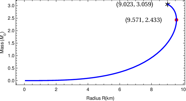
In Figure 12, we have analyzed the mass-radius (M-R) relationship obtained from the model. The red dot in the figure represents the maximum radius of star and the star marker represents the maximum mass permitted by the model. From the figure it can be noticed that the maximum radius is 9.571 kms and the corresponding star mass is 2.433 $M_{\odot}$, while the maximum permitted mass is 3.059 $M_{\odot}$ and the corresponding radius is 9.023 kms.
The present model is in good agreement with the mass and size of the star 4U 1820-30 and satisfy all the physical acceptability conditions with $\alpha$ in the range $0.157156\leq\alpha\leq 0.192717$.

We have examined our model with stars like PSR J1903+327, Vela X-1, Her X-1, SAX J1808.4-3658 and found that the model is in good agreement with the mass and radius of these stars given by Gangopadhyay et al. (2013). The valid ranges of the parameter $\alpha$ for which all the physical, regularity and energy conditions are satisfied, are displayed in Table 1.

Thus we have physically acceptable models of superdense stars with linear equation of state and a definite 3-space geometry, viz., the paraboloidal spacetime geometry. The present model is mathematically interesting as it has got a definite geometry and physically interesting because the spacetime with linear equation of state may be good candidate for representing strange stars.

References

- Abreu et al. [2007] H. Abreu, H. Hernández, and L. A. Núñez. Class. Quantum Grav., 24:4631, 2007.
- Bowers and Liang [1974] R. Bowers and E. Liang. Astrophys. J., 188:657, 1974.
- Buchdahl [1979] H. A. Buchdahl. Acta Phys. Pol., 10:673, 1979.
- Canuto [1974] V. Canuto. Annu. Rev. Astron. Astrophys., 12:167, 1974.
- Dayanandan et al. [2016] Baiju Dayanandan, S. K. Maurya, Y. K. Gupta, and T. T. Smitha. Astrophys Space Sci, 361:160, 2016.
- Delgaty and Lake [1998] M. S. R. Delgaty and K. Lake. Comput. Phys. Commun., 115:395, 1998.
- Dev and Gleiser [2002] K. Dev and M. Gleiser. Gen. Rel. Grav., 34:1793, 2002.
- Dev and Gleiser [2003] K. Dev and M. Gleiser. Gen. Rel. Grav., 35:1435.10, 2003.
- Dev and Gleiser [2004] K. Dev and M. Gleiser. Int. J. Mod. Phys. D, 13:1389, 2004.
- Dey et al. [1998] M. Dey, I. Bombaci, J. Dey, S. Ray, and B. C. Samanta. Phys. Lett. B, 438:123, 1998.
- Fatema and Murad [2013] S. Fatema and M. H. Murad. Int. J. Theor. Phys., 52:4342, 2013.
- Feroze and Siddiqui [2011] T. Feroze and A. A. Siddiqui. Gen. Relativ. Grav., 43:1025, 2011.
- Finch and Skea [1989] M. R. Finch and J. E. F. Skea. Class. Quantum Gravity, 6:467, 1989.
- Gangopadhyay et al. [2013] T. Gangopadhyay, S. Ray, X-D. Li, J. Dey, and M. Dey. Mon. Not. R. Astron. Soc., 431:3216, 2013.
- Gokhroo and Mehra [1994] M. K. Gokhroo and A. L. Mehra. Gen. Rel. Grav., 26:75, 1994.
- Gondek-Rosińska et al. [2000] D. Gondek-Rosińska, T. Bulik, L. Zdunik, E. Gourgoulhon, S. Ray, J. Dey, and M. Dey. Astron. & Astrophys., 363:1005, 2000.
- Ivanov [2002] B. V. Ivanov. Phys. Rev. D, 65:104011, 2002.
- Jotania and Tikekar [2006] K. Jotania and R. Tikekar. Int. J. Mod. Phys. D, 15:1175, 2006.
- Knutsen [1987] H. Knutsen. Astrophys Space Sci, 149:38, 1987.
- Kuchowicz [1972] B. Kuchowicz. Phys. Lett. A, 38:1972, 1972. doi: 10.1016/03759601(72)90164-8.
- Maharaj and Maartens [1989] S. D. Maharaj and R. Maartens. Gen. Rel. Grav., 21:899, 1989.
- Maharaj and Takisa [2012] S. D. Maharaj and P. M. Takisa. Gen. Rel. Grav., 44:1419, 2012.
- Maharaj and Takisa [2013] S. D. Maharaj and P. M. Takisa. Gen. Relativ. Grav., 45:1951, 2013.
- Maurya and Gupta [2011a] S. K. Maurya and Y. K. Gupta. Astrophys. Space Sci., 331:135, 2011a.
- Maurya and Gupta [2011b] S. K. Maurya and Y. K. Gupta. Astrophys Space Sci, 332:155, 2011b.
- Maurya and Gupta [2011c] S. K. Maurya and Y. K. Gupta. Astrophys Space Sci, 333:415, 2011c.
- Maurya et al. [2015a] S. K. Maurya, Y. K. Gupta, and S. Ray. arXiv:1502.01915 [gr-qc], 2015a.
- Maurya et al. [2015b] S. K. Maurya, Y. K. Gupta, Saibal Ray, and Baiju Dayanandan. Eur. Phys. J. C, 75:225, 2015b.
- Maurya et al. [2016a] S. K. Maurya, Y. K. Gupta, Baiju Dayanandan, and Saibal Ray. Eur. Phys. J. C, 76:266, 2016a.
- Maurya et al. [2016b] S. K. Maurya, Y. K. Gupta, T. T. Smitha, and F. Rahaman. Eur. Phys. J. A, 52:191, 2016b. doi: 10.1140/epja/i2016-16191-1.
- Maurya et al. [2016c] S. K. Maurya, M. K. Jasim, Y. K. Gupta, and T. T. Smitha. Astrophys Space Sci, 361:163, 2016c.
- Maurya et al. [2017] S. K. Maurya, Y. K. Gupta, Baiju Dayanandan, M. K. Jasim, and Ahmed Al-Jamel. Int. J. Mod. Phys. D, 26:1750002, 2017.
- Misner and Sharp [1964] C. Misner and D. Sharp. Phys. Rev. B, 136:571, 1964.
- Murad [2013a] M. H. Murad. Astrophys Space Sci, 343:187, 2013a.
- Murad [2013b] M. H. Murad. Astrophys Space Sci, 344:69, 2013b.
- Murad and Fatema [2013] M. H. Murad and S. Fatema. Int. J. Theor. Phys., 52:2508, 2013.
- Murad and Fatema [2014] M. H. Murad and S. Fatema. arXiv:1408.5126v2, 2014.
- Murad and Fatema [2015] M. H. Murad and S. Fatema. Eur. Phys. J. C, 75:533, 2015.
- Ngubelanga et al. [2015] S. A. Ngubelanga, S. D. Maharaj, and S. Ray. Astrophys Space Sci, 357:40, 2015.
- Pandya et al. [2015] D. M. Pandya, V. O. Thomas, and R. Sharma. Astrophys Space Sci, 356:285, 2015.
- Patel and Mehta [1995] L. K. Patel and N. P. Mehta. Austral. J. Phys., 48:635, 1995.
- Ratanpal et al. [2015a] B. S. Ratanpal, V. O. Thomas, and D. M. Pandya. Astrophys Space Sci, 360:53, 2015a.
- Ratanpal et al. [2015b] B. S. Ratanpal, V. O. Thomas, and D. M. Pandya. Astrophys Space Sci, 361:65, 2015b.
- Ruderman [1972] R. Ruderman. Astro. Astrophys., 10:427, 1972.
- Sharma and Maharaj [2007] R. Sharma and S. D. Maharaj. MNRAS, 375:1265, 2007.
- Sharma and Ratanpal [2013] R. Sharma and B. S. Ratanpal. Int. J. Mod. Phys. D, 13:1350074, 2013.
- Thirukkanesh and Ragel [2012] S. Thirukkanesh and F. S. Ragel. Pramana J. Phys., 78:687, 2012.
- Thomas and Pandya [2015a] V. O. Thomas and D. M. Pandya. Astrophys Space Sci, 360:39, 2015a.
- Thomas and Pandya [2015b] V. O. Thomas and D. M. Pandya. Astrophys Space Sci, 360:59, 2015b.
- Thomas and Ratanpal [2007] V. O. Thomas and B. S. Ratanpal. Int. J. Mod. Phys. D, 16:9, 2007.
- Thomas et al. [2005] V. O. Thomas, B. S. Ratanpal, and P. C. Vinodkumar. Int. J. Mod. Phys. D, 14:85, 2005.
- Tikekar and Thomas [1998] R. Tikekar and V. O. Thomas. Pramana- J. of phys., 50:95, 1998.
- Tikekar and Thomas [1999] R. Tikekar and V. O. Thomas. Pramana- J. of phys., 52:237, 1999.
- Tikekar and Thomas [2005] R. Tikekar and V. O. Thomas. Pramana- J. of phys., 64:5, 2005.
- Zdunik [2000] J. L. Zdunik. Astron. & Astrophys., 359:311, 2000.