跳到论文正文
W Papers独立论文阅读器 arXiv:1612.04847 论文正文 计算阅读时间 · 0%
引用这篇论文根据当前论文元数据生成,正式投稿前建议核对。


License: arXiv.org perpetual non-exclusive license
arXiv:1612.04847v3 [math.OC] 08 Nov 2017

Sensitivity and Covariance in Stochastic Complementarity Problems with an Application to North American Natural Gas Markets

Sriram Sankaranarayanan Email: ssankar5@jhu.edu Address: Department of Civil Engineering, Johns Hopkins University Corresponding author: Corresponding Author: ssankar5@jhu.edu    Felipe Feijoo Email: felipe.feijoo@pnnl.gov Address: Pontificia Universidad Católica de Valparaíso, Chile    Sauleh Siddiqui Email: siddiqui@jhu.edu Address: Department of Civil Engineering, Johns Hopkins University Address: Department of Applied Mathematics and Statistics, Johns Hopkins University Address: German Institute for Economic Research (DIW Berlin)
Abstract

We provide an efficient method to approximate the covariance between decision variables and uncertain parameters in solutions to a general class of stochastic nonlinear complementarity problems. We also develop a sensitivity metric to quantify uncertainty propagation by determining the change in the variance of the output due to a change in the variance of an input parameter. The covariance matrix of the solution variables quantifies the uncertainty in the output and pairs correlated variables and parameters. The sensitivity metric helps in identifying the parameters that cause maximum fluctuations in the output. The method developed in this paper optimizes the use of gradients and matrix multiplications which makes it particularly useful for large-scale problems. Having developed this method, we extend the deterministic version of the North American Natural Gas Model (NANGAM), to incorporate effects due to uncertainty in the parameters of the demand function, supply function, infrastructure costs, and investment costs. We then use the sensitivity metrics to identify the parameters that impact the equilibrium the most.

Keywords: 
Stochastic Programming, Large scale optimization , Complementarity problems , Approximation methods

1 Introduction

Complementarity models arise naturally out of various real life problems. A rigorous survey of their application is available in Ferris and Pang [1997]. Authors in Martín et al. [2015], Huppmann and Egging [2014], Feijoo et al. [2016], Oke et al. [2016], Abada et al. [2013], Christensen and Siddiqui [2015] use complementarity problems to model markets from a game theoretic perspective [Siddiqui and Christensen, 2016, Anderson and Xu, 2004], where the complementarity conditions typically arise between the marginal profit and the quantity produced by the producer. In the field of mechanics, they typically arise in the context of frictional contact problems [Kwak and Lee, 1988], where there is a complementarity relation between the frictional force between a pair of surfaces and the distance of separation between them. With a wide range of applications, understanding the characteristics of solutions to complementarity problems becomes important for advancing the field. In this paper, we focus on studying the characteristics of solutions to complementarity problems under uncertainty.

The behavior of a solution to a complementarity problem with random parameters was first addressed in Gürkan and Robinson [1999], where such problems were referred to as stochastic complementarity problems (SCP). Authors in Shanbhag [2013], Chen and Fukushima [2005], Gabriel et al. [2009], Egging et al. [2016], Jiang and Xu [2008] define various formulations of SCP for different applications and have devised algorithms to solve the problem. Authors in Lamm et al. [2016] compute confidence intervals for solution of the expected value formulation of the problem, however they do not have efficient methods to find the second-order statistics for large-scale complementarity problems.

Large-scale problems, those with over 10,000 decision variables and uncertain parameters arise naturally out of detailed market models and there is considerable interest in studying, understanding and solving such models. For example, Chen et al. [2017] discuss a case of urban drainage system with large number of variables. Yumashev and Johnson [2017] discuss a case of deciding under large-scale nuclear emergencies. In line with the area of application used in this paper, Gabriel et al. [2001] discuss a case of an energy model with large number of variables and parameters. Naturally, developing methods to solve such large-scale problems gained interest. Authors in Kopanos et al. [2010], Luo et al. [2015] discuss various tools ranging from mathematical techniques (decomposition based) to computational techniques (parallel processing) for solving large-scale optimization problems. Ohno et al. [2016] uses an approximate algorithm for a large-scale Markov decision process to optimize production and distribution systems. In this paper, we do not present a new method to solve stochastic complementarity problems, but an efficient algorithm to generate second-order information that is flexible enough to be coupled with any existing algorithm that provides a first-order solution.

The objective of this paper is to efficiently obtain second-order statistical information about solution vectors of large-scale stochastic complementarity problems. This gives us information about variability of the equilibrium obtained by solving a nonlinear complementarity problem (NCP) and the correlation between various variables in the solution. Authors in Hyett et al. [2007] and Benedetti-Cecchi [2003] provide examples in the area of clinical pathways and ecology respectively, about the utility of understanding the variance of the solution in addition to the mean. They also show that a knowledge of variance aids better understanding and planning of the system. Agrawal et al. [2012] emphasize the necessity to understand covariance as a whole rather than individual variances by quantifying “the loss incurred on ignoring correlations” in a stochastic programming model.

In addition, we also introduce a sensitivity metric which quantifies the change in uncertainty in the output due to a perturbation in the variance of uncertain input parameters. This helps us to directly compare input parameters by the amount of uncertainty they propagate to the solution.

In attaining the above objectives, the most computationally expensive step is to solve a system of linear equations. We choose approximation methods over analytical methods, integration, or Monte Carlo simulation because of the computational hurdle involved while implementing those methods for large-scale problems. The method we describe in this paper achieves the following:

  • 1.

    The most expensive step has to be performed just once, irrespective of the covariance of the input parameters. Once the linear system of equations is solved, for each given covariance scenario, we only perform two matrix multiplications.

  • 2.

    Approximating the covariance matrix and getting a sensitivity metric can be obtained by solving the above mentioned linear system just once.

The methods developed in this paper can also be used for nonlinear optimization problems with linear equality constraints. We prove stronger results on error bounds for special cases of quadratic programming.

Having developed this method, we apply it to a large-scale stochastic natural gas model for North America, an extension of the deterministic model developed in Feijoo et al. [2016] and determine the covariance of the solution variables. We then proceed to identify the parameters which have the greatest impact on the solution. A Python class for efficiently storing and operating on sparse arrays of dimension greater than two is created. This is useful for working with high-dimensional problems which have an inherent sparse structure in the gradients.

We divide the paper as follows. Section 2 formulates the problem and mentions the assumptions used in the paper. It then develops the algorithm used to approximate the solution covariance and provides proofs for bounding the error. Section 3 develops a framework to quantify the sensitivity of the solution to each of the random variables. Section 4 shows how the result can be applied for certain optimization problems with equality constraints. Having obtained the theoretical results, section 5 gives an example of a oligopoly where this method can be applied and compares the computational time of the approximation method with a Monte-Carlo method showing the performance improvement for large-scale problems. Section 6 describes the Natural Gas Model to which the said method is applied. Section 7 discusses the possible enhancements for the model and its limitations in the current form.

2 Approximation of covariance

For the rest of the paper, all bold quantities are vectors. A subscript ii for those quantities refer to the ii-th component of the vector in Cartesian representation.

2.1 Definitions

We define a complementarity problem and a stochastic complementarity problem which are central to the results obtained in this paper. We use a general definition of complementarity problems and stochastic complementarity problems as stated below.

Definition 1.

[Facchinei and Pang, 2007] Given 𝐅:ℝn×m↦ℝn{\color[rgb]{0,0,0}\mathbf{{\color[rgb]{0,0,0}\mathbf{F}}}}:\mathbb{R}^{n\times m}\mapsto\mathbb{R}^{n}, and parameters θ∈ℝm{\mathbf{{\theta}}}\in\mathbb{R}^{m}, the parametrized nonlinear complementarity problem (NCP) is to find 𝐱∈ℝn{\mathbf{x}}\in\mathbb{R}^{n} such that

𝕂∋𝐱⟂𝐅⁡(𝐱,θ)∈𝕂∗\displaystyle\mathbb{K}\ni{\mathbf{x}}\perp{\color[rgb]{0,0,0}\mathbf{{\color[rgb]{0,0,0}\mathbf{F}}}}({\mathbf{x}};{\mathbf{{\theta}}})\in\mathbb{K}^{*} (2.1)

where 𝕂∗\mathbb{K}^{*}, the dual cone of 𝕂\mathbb{K} is defined as

𝕂∗\displaystyle\mathbb{K}^{*}\quad ={𝐱∈ℝn:𝐯T𝐱≥0∀𝐯∈𝕂}\displaystyle=\quad\left\{{\mathbf{x}}\in\mathbb{R}^{n}:\mathbf{v}^{T}{\mathbf{x}}\geq 0\quad\forall\mathbf{v}\in\mathbb{K}\right\} (2.2)
Definition 2.

Given a cone 𝕂∈ℝn\mathbb{K}\in\mathbb{R}^{n} a random function 𝐅:𝕂×Ω↦ℝn{\color[rgb]{0,0,0}\mathbf{{\color[rgb]{0,0,0}\mathbf{F}}}}:\mathbb{K}\times\Omega\mapsto\mathbb{R}^{n}, the stochastic complementarity problem (SCP) is to find x∈ℝnx\in\mathbb{R}^{n} such that

𝕂∋𝐱⟂𝔼𝐅​(𝐱,ω)∈𝕂∗\displaystyle\mathbb{K}\ni{\mathbf{x}}\perp\expec{\color[rgb]{0,0,0}\mathbf{{\color[rgb]{0,0,0}\mathbf{F}}}}({\mathbf{x}};{\color[rgb]{0,0,0}\omega})\in\mathbb{K}^{*} (2.3)

We assume that we can explicitly evaluate the expectation in (2.3) using its functional form, and that the SCP can be solved using an existing algorithm.

We now make assumptions on the form of 𝕂\mathbb{K} in (2.1). This form of 𝕂\mathbb{K} helps in establishing an equivalence between a complementarity problem and a minimization problem which is key to derive the approximation method in this paper.

Assumption 1.

𝕂\mathbb{K} in (2.1) is a Cartesian product of half spaces and full spaces, i.e., for some ℐ⊆{1,2,…,n}\mathcal{I}\subseteq\left\{1,2,\ldots,n\right\}

𝕂\displaystyle\mathbb{K}\quad ={𝐱∈ℝn:𝐱i≥0if i∈ℐ}\displaystyle=\quad\left\{{\mathbf{x}}\in\mathbb{R}^{n}:\quad{\mathbf{x}}_{i}\geq 0\quad\mbox{if }i\in\mathcal{I}\right\} (2.4)

We now propose a lemma about the form of the dual cone of 𝕂\mathbb{K} to understand the special form that it has. This will help us convert the complementarity problem into an unconstrained minimization problem.

Lemma 3.

The dual cone 𝕂∗\mathbb{K}^{*} of the set assumed in assumption 1 is

𝕂∗=𝕂′\displaystyle\mathbb{K}^{*}=\mathbb{K}^{\prime} ={𝐱∈ℝn:𝐱i≥0 if ​i∈ℐ𝐱i=0 if ​i∉ℐ}\displaystyle=\left\{{\mathbf{x}}\in\mathbb{R}^{n}:\begin{array}[]{lr}{\mathbf{x}}_{i}\geq 0&\mbox{ if }i\in\mathcal{I}\\ {\mathbf{x}}_{i}=0&\mbox{ if }i\not\in\mathcal{I}\\ \end{array}\right\}
Proof.

Check Appendix A∎

2.2 Preliminaries for approximation

In this subsection, we prove two preliminary results. Firstly, we prove our ability to pose an NCP as an unconstrained minimization problem. Then we prove results on twice continuous differentiability of the objective function, thus enabling us to use the rich literature available for smooth unconstrained minimization. Following that, propositions 5 and 6 help in achieving the former while proposition 7 along with its corollaries help us in achieving the latter.

We now define C-functions, which are central to pose the complementarity problem into an unconstrained optimization problem. The equivalent formulation as an unconstrained optimization problem assists us in developing the algorithm.

Definition 4.

[Facchinei and Pang, 2007, Pg.  72] A function ψ:ℝ2↦ℝ{\color[rgb]{0,0,0}\psi}:\mathbb{R}^{2}\mapsto\mathbb{R} is a C-function when

ψ⁡(x,y)=0⇔x≥0y≥0xy=0\displaystyle\begin{split}{\color[rgb]{0,0,0}\psi}(x,y)=0\qquad&\Leftrightarrow\qquad x\geq 0\quad y\geq 0\quad xy=0\end{split} (2.7)

We consider the following commonly used C-functions.

ψF​B​(x,y)\displaystyle{\color[rgb]{0,0,0}\psi}_{FB}(x,y)\quad =x2+y2−x−y\displaystyle=\quad\sqrt{x^{2}+y^{2}}-x-y (2.8)
ψm​i​n​(x,y)\displaystyle{\color[rgb]{0,0,0}\psi}_{min}(x,y)\quad =min⁡(x,y)\displaystyle=\quad\min(x,y) (2.9)

Under our assumptions on 𝕂\mathbb{K}, the following two propositions establish the equivalence of the complementarity problem and an unconstrained minimization problem.

Proposition 5.

Suppose assumption 1 holds. Then every solution 𝐱∗​(θ){\color[rgb]{0,0,0}{\mathbf{x}}^{*}}({\mathbf{{\theta}}}) of the parameterized complementarity problem in (2.1), is a global minimum of the following function 𝖿⁡(𝐱,θ){\color[rgb]{0,0,0}\mathsf{f}}({\mathbf{x}};{\mathbf{{\theta}}}),

Φi​(𝐱,θ,𝐅)\displaystyle{\color[rgb]{0,0,0}\Phi}_{i}({\mathbf{x}},{\mathbf{{\theta}}};{\color[rgb]{0,0,0}\mathbf{{\color[rgb]{0,0,0}\mathbf{F}}}})\quad ={𝐅i​(𝐱,θ)if i∉ℐψi​(𝐱i,𝐅i​(𝐱,θ))if i∈ℐ\displaystyle=\quad\left\{\begin{array}[]{ll}{\color[rgb]{0,0,0}\mathbf{{\color[rgb]{0,0,0}\mathbf{F}}}}_{i}({\mathbf{x}},{\mathbf{{\theta}}})&\qquad\mbox{if }\quad i\not\in\mathcal{I}\\ {\color[rgb]{0,0,0}\psi}_{i}({\mathbf{x}}_{i},{\color[rgb]{0,0,0}\mathbf{{\color[rgb]{0,0,0}\mathbf{F}}}}_{i}({\mathbf{x}},{\mathbf{{\theta}}}))&\qquad\mbox{if }\quad i\in\mathcal{I}\end{array}\right.
𝖿⁡(𝐱,θ)\displaystyle{\color[rgb]{0,0,0}\mathsf{f}}({\mathbf{x}};{\mathbf{{\theta}}})\quad =12​‖Φ⁡(𝐱,θ,𝐅)‖22\displaystyle=\quad\frac{1}{2}\|{\color[rgb]{0,0,0}\Phi}({\mathbf{x}};{\mathbf{{\theta}}};{\color[rgb]{0,0,0}\mathbf{{\color[rgb]{0,0,0}\mathbf{F}}}})\|_{2}^{2} (2.12)

with an objective value 0, for some set of not necessarily identical C-functions ψi{\color[rgb]{0,0,0}\psi}_{i}.

Proof.

Check Appendix A∎

Proposition 6.

Suppose assumption 1 holds. If a solution to the problem in (2.1) exists and 𝐱∗​(θ){\color[rgb]{0,0,0}{\mathbf{x}}^{*}}({\mathbf{{\theta}}}) is an unconstrained global minimizer of 𝖿⁡(𝐱,θ){\color[rgb]{0,0,0}\mathsf{f}}({\mathbf{x}};{\mathbf{{\theta}}}) defined in (2.12), then 𝐱∗​(θ){\color[rgb]{0,0,0}{\mathbf{x}}^{*}}({\mathbf{{\theta}}}) solves the complementarity problem in (2.1).

Proof.

Check Appendix A∎

Now given a function 𝐅{\color[rgb]{0,0,0}\mathbf{{\color[rgb]{0,0,0}\mathbf{F}}}}, and a set 𝕂\mathbb{K} which satisfies assumption 1, and a solution of the NCP 𝐱∗​(θ^){\color[rgb]{0,0,0}{\mathbf{x}}^{*}}({\color[rgb]{0,0,0}\hat{{\mathbf{{\theta}}}}}) for some fixed θ=θ^{\mathbf{{\theta}}}={\color[rgb]{0,0,0}\hat{{\mathbf{{\theta}}}}}, we define a vector valued function Φ:ℝn×m↦ℝn{\color[rgb]{0,0,0}\Phi}:\mathbb{R}^{n\times m}\mapsto\mathbb{R}^{n} component-wise as follows.

Φi​(𝐱,θ,𝐅)\displaystyle{\color[rgb]{0,0,0}\Phi}_{i}({\mathbf{x}},{\mathbf{{\theta}}};{\color[rgb]{0,0,0}\mathbf{{\color[rgb]{0,0,0}\mathbf{F}}}})\quad ={𝐅i​(𝐱,θ)if i∉ℐψ2​(𝐱i,𝐅i​(𝐱,θ))if i∈𝒵ψ⁡(𝐱i,𝐅i​(𝐱,θ))otherwise\displaystyle=\quad\left\{\begin{array}[]{ll}{\color[rgb]{0,0,0}\mathbf{{\color[rgb]{0,0,0}\mathbf{F}}}}_{i}({\mathbf{x}},{\mathbf{{\theta}}})&\qquad\mbox{if }\quad i\not\in\mathcal{I}\\ {\color[rgb]{0,0,0}\psi}^{2}({\mathbf{x}}_{i},{\color[rgb]{0,0,0}\mathbf{{\color[rgb]{0,0,0}\mathbf{F}}}}_{i}({\mathbf{x}},{\mathbf{{\theta}}}))&\qquad\mbox{if }\quad i\in\mathcal{Z}\\ {\color[rgb]{0,0,0}\psi}({\mathbf{x}}_{i},{\color[rgb]{0,0,0}\mathbf{{\color[rgb]{0,0,0}\mathbf{F}}}}_{i}({\mathbf{x}},{\mathbf{{\theta}}}))&\qquad\mbox{otherwise}\end{array}\right.
𝖿⁡(𝐱,θ)\displaystyle{\color[rgb]{0,0,0}\mathsf{f}}({\mathbf{x}};{\mathbf{{\theta}}})\quad =12​‖Φ⁡(𝐱,θ,𝐅)‖22\displaystyle=\quad\frac{1}{2}\|{\color[rgb]{0,0,0}\Phi}({\mathbf{x}};{\mathbf{{\theta}}};{\color[rgb]{0,0,0}\mathbf{{\color[rgb]{0,0,0}\mathbf{F}}}})\|_{2}^{2} (2.16)
𝒵\displaystyle\mathcal{Z}\quad ={i∈ℐ:𝐱∗i​(θ^)=𝐅i​(𝐱∗​(θ^),θ^)=0}\displaystyle=\quad\left\{i\in\mathcal{I}:{\color[rgb]{0,0,0}{\mathbf{x}}^{*}}_{i}({\color[rgb]{0,0,0}\hat{{\mathbf{{\theta}}}}})={\color[rgb]{0,0,0}\mathbf{F}}_{i}({\color[rgb]{0,0,0}{\mathbf{x}}^{*}}({\color[rgb]{0,0,0}\hat{{\mathbf{{\theta}}}}});{\color[rgb]{0,0,0}\hat{{\mathbf{{\theta}}}}})=0\right\} (2.17)

Note that if ψ{\color[rgb]{0,0,0}\psi} is a C-function, ψ2{\color[rgb]{0,0,0}\psi}^{2} is also a C-function since ψ2=0⇔ψ=0{\color[rgb]{0,0,0}\psi}^{2}=0\iff{\color[rgb]{0,0,0}\psi}=0. We observe from propositions 5 and 6 that minimizing 𝖿⁡(𝐱,θ){\color[rgb]{0,0,0}\mathsf{f}}({\mathbf{x}};{\mathbf{{\theta}}}) over 𝐱{\mathbf{x}} is equivalent to solving the NCP in (2.1).

Now we assume conditions on the smoothness of 𝐅{\color[rgb]{0,0,0}\mathbf{{\color[rgb]{0,0,0}\mathbf{F}}}} so that the solution to a perturbed problem is sufficiently close to the original solution.

Assumption 2.

𝐅⁡(𝐱,θ){\color[rgb]{0,0,0}\mathbf{{\color[rgb]{0,0,0}\mathbf{F}}}}({\mathbf{x}};{\mathbf{{\theta}}}) is twice continuously differentiable in 𝐱{\mathbf{x}} and θ{\mathbf{{\theta}}} over an open set containing 𝕂\mathbb{K}.

Given that the rest of the analysis is on the function 𝖿⁡(𝐱,θ){\color[rgb]{0,0,0}\mathsf{f}}({\mathbf{x}};{\mathbf{{\theta}}}) defined in (2.16), we prove that a sufficiently smooth 𝐅{\color[rgb]{0,0,0}\mathbf{{\color[rgb]{0,0,0}\mathbf{F}}}} and a suitable ψ{\color[rgb]{0,0,0}\psi} ensure a sufficiently smooth 𝖿{\color[rgb]{0,0,0}\mathsf{f}}.

Proposition 7.

With assumption 2 holding, we state 𝖿⁡(𝐱,θ^){\color[rgb]{0,0,0}\mathsf{f}}({\mathbf{x}};{\color[rgb]{0,0,0}\hat{{\mathbf{{\theta}}}}}) defined as in (2.16) is a twice continuously differentiable at 𝐱{\mathbf{x}} satisfying 𝖿⁡(𝐱,θ^)=0{\color[rgb]{0,0,0}\mathsf{f}}({\mathbf{x}};{\color[rgb]{0,0,0}\hat{{\mathbf{{\theta}}}}})=0 for any C function ψ{\color[rgb]{0,0,0}\psi} provided

  1. 1.

    ψ{\color[rgb]{0,0,0}\psi} is twice differentiable at {(a,b)∈ℝ2:ψ⁡(a,b)=0}∖{(0,0)}\left\{(a,b)\in\mathbb{R}^{2}:{\color[rgb]{0,0,0}\psi}(a,b)=0\right\}\setminus\{(0,0)\} with a finite derivative and finite second derivative.

  2. 2.

    ψ{\color[rgb]{0,0,0}\psi} vanishes sufficiently fast near the origin. i.e.,

    lim(a,b)→(0,0)ψ2​(a,b)​∂2ψ⁡(a,b)∂a​∂b\displaystyle\lim_{(a,b)\rightarrow(0,0)}{\color[rgb]{0,0,0}\psi}^{2}(a,b)\frac{\partial^{2}{\color[rgb]{0,0,0}\psi}(a,b)}{\partial a\partial b}\quad =0\displaystyle=\quad 0 (2.18)
Proof.

Given that 𝖿{\color[rgb]{0,0,0}\mathsf{f}} is a sum of squares, it is sufficient to prove each term individually is twice continuously differentiable to prove the theorem. Also since we are only interested where 𝖿{\color[rgb]{0,0,0}\mathsf{f}} vanishes, it is sufficient to prove the above property for each term where it vanishes.
Consider terms from i∉ℐi\not\in\mathcal{I}. Since 𝐅i{\color[rgb]{0,0,0}\mathbf{F}}_{i} is twice continuously differentiable, 𝐅i2{\color[rgb]{0,0,0}\mathbf{F}}_{i}^{2} is twice continuously differentiable too.
Consider the case i∈𝒵i\in\mathcal{Z}. This means i∈ℐi\in\mathcal{I} and 𝐱∗i​(θ^)=𝐅i​(𝐱∗i​(θ^),θ^)=0{\color[rgb]{0,0,0}{\mathbf{x}}^{*}}_{i}({\color[rgb]{0,0,0}\hat{{\mathbf{{\theta}}}}})={\color[rgb]{0,0,0}\mathbf{F}}_{i}\left({\color[rgb]{0,0,0}{\mathbf{x}}^{*}}_{i}({\color[rgb]{0,0,0}\hat{{\mathbf{{\theta}}}}}),{\color[rgb]{0,0,0}\hat{{\mathbf{{\theta}}}}}\right)=0. These contribute a ψ4{\color[rgb]{0,0,0}\psi}^{4} term to 𝖿{\color[rgb]{0,0,0}\mathsf{f}}. With the notation ψi≡ψ⁡(𝐱i,𝐅i​(𝐱,θ)){\color[rgb]{0,0,0}\psi}_{i}\equiv{\color[rgb]{0,0,0}\psi}({\mathbf{x}}_{i},{\color[rgb]{0,0,0}\mathbf{F}}_{i}({\mathbf{x}};{\mathbf{{\theta}}})), and δi​j=1⇔i=j\delta_{ij}=1\iff i=j and 00 otherwise we clearly have,

∂ψi4∂𝐱j\displaystyle\frac{\partial{\color[rgb]{0,0,0}\psi}^{4}_{i}}{\partial{\mathbf{x}}_{j}}\quad =4​ψi3​(∂ψi∂a​δi​j+∂ψi∂b​∂𝐅i∂𝐱j)=0\displaystyle=\quad 4{\color[rgb]{0,0,0}\psi}^{3}_{i}\left(\frac{\partial{\color[rgb]{0,0,0}\psi}_{i}}{\partial a}\delta_{ij}+\frac{\partial{\color[rgb]{0,0,0}\psi}_{i}}{\partial b}\frac{\partial{\color[rgb]{0,0,0}\mathbf{F}}_{i}}{\partial{\mathbf{x}}_{j}}\right)\quad=\quad 0 (2.19)
∂2ψi4∂𝐱j​𝐱k\displaystyle\frac{\partial^{2}{\color[rgb]{0,0,0}\psi}^{4}_{i}}{\partial{\mathbf{x}}_{j}{\mathbf{x}}_{k}}\quad =12​ψi2​(∂ψi∂a​δi​j+∂ψi∂b​∂𝐅i∂𝐱j)​(∂ψi∂a​δi​k+∂ψi∂b​∂𝐅i∂𝐱k)\displaystyle=\quad 12{\color[rgb]{0,0,0}\psi}^{2}_{i}\left(\frac{\partial{\color[rgb]{0,0,0}\psi}_{i}}{\partial a}\delta_{ij}+\frac{\partial{\color[rgb]{0,0,0}\psi}_{i}}{\partial b}\frac{\partial{\color[rgb]{0,0,0}\mathbf{F}}_{i}}{\partial{\mathbf{x}}_{j}}\right)\left(\frac{\partial{\color[rgb]{0,0,0}\psi}_{i}}{\partial a}\delta_{ik}+\frac{\partial{\color[rgb]{0,0,0}\psi}_{i}}{\partial b}\frac{\partial{\color[rgb]{0,0,0}\mathbf{F}}_{i}}{\partial{\mathbf{x}}_{k}}\right)
+4​ψi3​(∂2ψi∂a2​δi​j​δi​k+∂2ψi∂a​∂b​∂𝐅i∂𝐱k+ other terms )\displaystyle\qquad\quad+4{\color[rgb]{0,0,0}\psi}^{3}_{i}\left(\frac{\partial^{2}{\color[rgb]{0,0,0}\psi}_{i}}{\partial a^{2}}\delta_{ij}\delta_{ik}+\frac{\partial^{2}{\color[rgb]{0,0,0}\psi}_{i}}{\partial a\partial b}\frac{\partial{\color[rgb]{0,0,0}\mathbf{F}}_{i}}{\partial{\mathbf{x}}_{k}}+\mbox{ other terms }\right) (2.20)
=0\displaystyle=\quad 0 (2.21)

For the third case, i∈ℐ∖𝒵i\in\mathcal{I}\setminus\mathcal{Z}, we have

∂ψi2∂𝐱j\displaystyle\frac{\partial{\color[rgb]{0,0,0}\psi}_{i}^{2}}{\partial{\mathbf{x}}_{j}}\quad =2​ψi​(∂ψi∂a​δi​j+∂ψi∂b​∂𝐅i∂𝐱j)=0\displaystyle=\quad 2{\color[rgb]{0,0,0}\psi}_{i}\left(\frac{\partial{\color[rgb]{0,0,0}\psi}_{i}}{\partial a}\delta_{ij}+\frac{\partial{\color[rgb]{0,0,0}\psi}_{i}}{\partial b}\frac{\partial{\color[rgb]{0,0,0}\mathbf{F}}_{i}}{\partial{\mathbf{x}}_{j}}\right)\quad=\quad 0 (2.22)
∂2ψi2∂𝐱j​𝐱k\displaystyle\frac{\partial^{2}{\color[rgb]{0,0,0}\psi}_{i}^{2}}{\partial{\mathbf{x}}_{j}{\mathbf{x}}_{k}}\quad =(∂ψi∂a​δi​j+∂ψi∂b​∂𝐅i∂𝐱j)\displaystyle=\quad\left(\frac{\partial{\color[rgb]{0,0,0}\psi}_{i}}{\partial a}\delta_{ij}+\frac{\partial{\color[rgb]{0,0,0}\psi}_{i}}{\partial b}\frac{\partial{\color[rgb]{0,0,0}\mathbf{F}}_{i}}{\partial{\mathbf{x}}_{j}}\right)
+2​ψi​(∂2ψi∂a2​δi​j​δi​k+∂2ψi∂a​∂b​∂𝐅i∂𝐱k+ other terms )\displaystyle\qquad\quad+2{\color[rgb]{0,0,0}\psi}_{i}\left(\frac{\partial^{2}{\color[rgb]{0,0,0}\psi}_{i}}{\partial a^{2}}\delta_{ij}\delta_{ik}+\frac{\partial^{2}{\color[rgb]{0,0,0}\psi}_{i}}{\partial a\partial b}\frac{\partial{\color[rgb]{0,0,0}\mathbf{F}}_{i}}{\partial{\mathbf{x}}_{k}}+\mbox{ other terms }\right) (2.23)
=∂ψi∂a​δi​j+∂ψi∂b​∂𝐅i∂𝐱j\displaystyle=\quad\frac{\partial{\color[rgb]{0,0,0}\psi}_{i}}{\partial a}\delta_{ij}+\frac{\partial{\color[rgb]{0,0,0}\psi}_{i}}{\partial b}\frac{\partial{\color[rgb]{0,0,0}\mathbf{F}}_{i}}{\partial{\mathbf{x}}_{j}} (2.24)

Continuity of 𝖿{\color[rgb]{0,0,0}\mathsf{f}} at the points of interest follow the continuity of the individual terms at the points. ∎

The following corollaries show the existence of C-functions ψ{\color[rgb]{0,0,0}\psi} which satisfy the hypothesis of proposition 7.

Corollary 8.

With assumption 2 holding, for the choice of C-function ψ=ψm​i​n{\color[rgb]{0,0,0}\psi}={\color[rgb]{0,0,0}\psi}_{min} defined in (2.9), the function 𝖿{\color[rgb]{0,0,0}\mathsf{f}} is twice continuously differentiable at its zeros.

Corollary 9.

With assumption 2 holding, for the choice of C-function ψ=ψF​B{\color[rgb]{0,0,0}\psi}={\color[rgb]{0,0,0}\psi}_{FB} defined in (2.8), the function 𝖿{\color[rgb]{0,0,0}\mathsf{f}} is twice continuously differentiable.

We now define an isolated solution to a problem and assume that the problem of interest has this property. This is required to ensure that our approximation is well defined.

Definition 10.

[Nocedal and Wright, 2006] A minimum 𝐱∗{\color[rgb]{0,0,0}{\mathbf{x}}^{*}} of a problem is said to be an isolated minimum, if there is a neighborhood ℬ⁡(𝐱∗,ϵ)\mathcal{B}({\color[rgb]{0,0,0}{\mathbf{x}}^{*}};\epsilon) of 𝐱∗{\color[rgb]{0,0,0}{\mathbf{x}}^{*}}, where 𝐱∗{\color[rgb]{0,0,0}{\mathbf{x}}^{*}} is the only minimum of the problem.

Refer to caption
(a) An example of a function where the global minimum x=0x=0 is a non-isolated solution
Refer to caption
(b) The intuition behind our approximation for finding where ∇𝖿​(𝐱,θ)=0\nabla{\color[rgb]{0,0,0}\mathsf{f}}({\mathbf{x}},{\mathbf{{\theta}}})=0 under a small perturbation
Figure 1: Intuitions

A counter-example for an isolated minimum is shown on Fig. 1(a). It is a plot of the function

f⁡(x)\displaystyle f(x)\quad =5​x2+x2​sin⁡(1x2)\displaystyle=\quad 5x^{2}+x^{2}\sin\left(\frac{1}{x^{2}}\right) (2.25)

and the global minimum at x=0x=0 is not an isolated minimum as we can confirm that any open interval around x=0x=0 has other minimum contained in it. Unlike this case, in this paper, we assume that if we obtain a global-minimum of 𝖿{\color[rgb]{0,0,0}\mathsf{f}}, then it is an isolated minimum. The existence of a neighborhood ℬ⁡(𝐱∗,ϵ)\mathcal{B}({\color[rgb]{0,0,0}{\mathbf{x}}^{*}};\epsilon) as required in definition 10 protects the approximation method from returning to a local minimum in the neighborhood for sufficiently small perturbations in problem parameters.

Assumption 3.

For some fixed value of θ=θ^{\mathbf{{\theta}}}={\color[rgb]{0,0,0}\hat{{\mathbf{{\theta}}}}}, there exists a known solution 𝐱∗​(θ^){\color[rgb]{0,0,0}{\mathbf{x}}^{*}}({\color[rgb]{0,0,0}\hat{{\mathbf{{\theta}}}}}) such that it is an isolated global minimum of 𝖿⁡(𝐱,θ){\color[rgb]{0,0,0}\mathsf{f}}({\mathbf{x}};{\mathbf{{\theta}}}).

2.3 Approximation Algorithm and error bounding

This subsection achieves two primary results as follows. We now propose algorithm 1 to approximate the covariance of the output given a covariance matrix for the input parameters. Following that Theorem 11 gives a mathematical proof that the algorithm indeed approximates the covariance matrix. The second key result is Theorem 12 which bounds the error in the approximation.

Given a deterministic shift in a parameter’s value, the sensitivity of the solution has been studied in Fiacco [2009], Castillo et al. [2006] for mathematical programming problems (e.g., nonlinear or large-scale programs). Authors in Castillo et al. [2008] used a perturbation technique to study the sensitivities in calculus of variations. We aim to build on the research in Fiacco [2009], Castillo et al. [2006] by proposing an approximation approach for large-scale stochastic complementarity problems. In particular, the sensitivity analysis in Chapter 3 in Fiacco [2009] motivates the method developed in this paper, after converting the complementarity problem into an unconstrained optimization problem with sufficient smoothness properties. Chapters 4 and 5 in Fiacco [2009] provide good context for computational approaches related to the ideas of Chapter 3. Our approach is amenable to extensions towards approximations for large-scale models, as we study the sensitivity of the variance of the solution, to a perturbation in the variance of input random parameters. We invite readers to refer to these works on further context in standard optimization problems. Chapter 2 of Fiacco [2009] provides interesting examples on how small perturbations can lead to large changes in solutions. This is good context in situations where Assumptions 2 (and Corollaries 8 and 9) and 3 in our paper do not hold. The research in Castillo et al. [2006] provides good context for standard optimization problems, including situations where we relax assumptions on smoothness and active constraints.

The intuition behind the approximation is shown on Fig. 1(b) and can be summarized as follows. Having posed the NCP as an unconstrained minimization of a function 𝖿{\color[rgb]{0,0,0}\mathsf{f}}, we now approximate the change in the solution due to a perturbation of the parameters. Keeping the smoothness properties of 𝖿{\color[rgb]{0,0,0}\mathsf{f}} in mind, we say that the gradient of 𝖿{\color[rgb]{0,0,0}\mathsf{f}} vanishes at the solution before any perturbation. Following the random perturbation of parameters, we approximate the new value of the gradient of 𝖿{\color[rgb]{0,0,0}\mathsf{f}} at the old solution. Then we compute the step to be taken so that the gradient at the new point vanishes. We formalize this idea in Theorem 11 and use that to build Algorithm 1 with some features for increased efficiency. The analysis builds on Dini’s implicit function theorem Krantz and Parks [2012] for deterministic perturbations and extends the results to predict covariance under random perturbations.

Algorithm 1 Approximating Covariance

Solve the complementarity problem in (2.1) for the mean value of θ=θ^{\mathbf{{\theta}}}={\color[rgb]{0,0,0}\hat{{\mathbf{{\theta}}}}}, or solve the stochastic complementarity problem in (2.3) and calibrate the value of the parameters θ=θ^{\mathbf{{\theta}}}={\color[rgb]{0,0,0}\hat{{\mathbf{{\theta}}}}} for this solution. Call this solution as 𝐱∗{\color[rgb]{0,0,0}{\mathbf{x}}^{*}}. Choose a tolerance level τ\tau.


1: Evaluate 𝐅∗←𝐅⁡(𝐱∗,θ^){{\color[rgb]{0,0,0}\mathbf{{\color[rgb]{0,0,0}\mathbf{F}}}}^{*}}\leftarrow{{\color[rgb]{0,0,0}\mathbf{{\color[rgb]{0,0,0}\mathbf{F}}}}({\color[rgb]{0,0,0}{\mathbf{x}}^{*}};{\color[rgb]{0,0,0}\hat{{\mathbf{{\theta}}}}})}, Gi​j←∂𝐅i​(𝐱∗,θ^)∂𝐱jG_{ij}\leftarrow\frac{\partial{\color[rgb]{0,0,0}\mathbf{F}}_{i}({\color[rgb]{0,0,0}{\mathbf{x}}^{*}};{\color[rgb]{0,0,0}\hat{{\mathbf{{\theta}}}}})}{\partial{\mathbf{x}}_{j}}, Li,j←∂𝐅i​(𝐱∗,θ^)∂θjL_{i,j}\leftarrow\frac{\partial{\color[rgb]{0,0,0}\mathbf{F}}_{i}({\color[rgb]{0,0,0}{\mathbf{x}}^{*}};{\color[rgb]{0,0,0}\hat{{\mathbf{{\theta}}}}})}{\partial{\mathbf{{\theta}}}_{j}}.
2: Choose a C-function ψ{\color[rgb]{0,0,0}\psi} such that the conditions in proposition 7 are satisfied.
3: Define the function ψa​(a,b)=∂ψ⁡(a,b)∂a{\color[rgb]{0,0,0}\psi}^{a}(a,b)=\frac{\partial{\color[rgb]{0,0,0}\psi}(a,b)}{\partial a}, ψb​(a,b)=∂ψ⁡(a,b)∂b{\color[rgb]{0,0,0}\psi}^{b}(a,b)=\frac{\partial{\color[rgb]{0,0,0}\psi}(a,b)}{\partial b}.
4: Find the set of indices 𝒵={z∈ℐ:|𝐱∗z|=|𝐅z∗|≤τ}\mathcal{Z}=\left\{z\in\mathcal{I}:|{\color[rgb]{0,0,0}{\mathbf{x}}^{*}}_{z}|=|{\color[rgb]{0,0,0}\mathbf{{\color[rgb]{0,0,0}\mathbf{F}}}}^{*}_{z}|\leq\tau\right\}.
5: Define
ℳi​j\displaystyle{\color[rgb]{0,0,0}\mathcal{M}}_{ij}\quad ←{Gi​j if ​i∉ℐ0 if ​i∈𝒵ψa​(𝐱∗i,𝐅i∗)​δi​j+ψb​(𝐱∗i,𝐅i∗)​Gi​j otherwise\displaystyle\leftarrow\quad\left\{\begin{array}[]{lr}G_{ij}&\mbox{ if }i\not\in\mathcal{I}\\ 0&\mbox{ if }i\in\mathcal{Z}\\ {\color[rgb]{0,0,0}\psi}^{a}({\color[rgb]{0,0,0}{\mathbf{x}}^{*}}_{i},{\color[rgb]{0,0,0}\mathbf{F}}^{*}_{i})\delta_{ij}+{\color[rgb]{0,0,0}\psi}^{b}({\color[rgb]{0,0,0}{\mathbf{x}}^{*}}_{i},{\color[rgb]{0,0,0}\mathbf{F}}^{*}_{i})G_{ij}&\mbox{ otherwise}\end{array}\right.
where δi​j=1\delta_{ij}=1 if i=ji=j and 0 otherwise.
6: Define
𝒩i​j\displaystyle\mathcal{N}_{ij}\quad ←{Li​j if ​i∉ℐ0 if ​i∈𝒵ψb​(𝐱∗i,𝐅i∗)​Li​j otherwise\displaystyle\leftarrow\quad\left\{\begin{array}[]{ll}L_{ij}&\mbox{ if }i\not\in\mathcal{I}\\ 0&\mbox{ if }i\in\mathcal{Z}\\ {\color[rgb]{0,0,0}\psi}^{b}({\color[rgb]{0,0,0}{\mathbf{x}}^{*}}_{i},{\color[rgb]{0,0,0}\mathbf{F}}_{i}^{*})L_{ij}&\mbox{ otherwise}\end{array}\right.
7: Solve the linear systems of equations for 𝒯{\color[rgb]{0,0,0}\mathcal{T}}.
ℳ​𝒯\displaystyle{\color[rgb]{0,0,0}\mathcal{M}}{\color[rgb]{0,0,0}\mathcal{T}}\quad =𝒩\displaystyle=\quad\mathcal{N} (2.32)
If ℳ{\color[rgb]{0,0,0}\mathcal{M}} is non singular, we have a unique solution. If not, a least square solution or a solution obtained by calculating the Moore Penrose Pseudo inverse [Horn and Johnson, 2012] can be used.
8: Given 𝒞\mathcal{C}, a covariance matrix of the input random parameters, θ⁡(ω){\mathbf{{\theta}}}({\color[rgb]{0,0,0}\omega}), return 𝒞∗←𝒯​𝒞​𝒯T\mathcal{C}^{*}\leftarrow{\color[rgb]{0,0,0}\mathcal{T}}\mathcal{C}{\color[rgb]{0,0,0}\mathcal{T}}^{T}.
Theorem 11.

Algorithm 1 generates Taylor’s first-order approximation for the change in solution for a perturbation in parameters and computes the covariance of the solution for a complementarity problem with uncertain parameters with small variances.

Proof.

Consider the function 𝖿⁡(𝐱,θ){\color[rgb]{0,0,0}\mathsf{f}}({\mathbf{x}};{\mathbf{{\theta}}}). From Theorem 5, 𝐱∗≡𝐱∗​(θ^){\color[rgb]{0,0,0}{\mathbf{x}}^{*}}\equiv{\color[rgb]{0,0,0}{\mathbf{x}}^{*}}({\color[rgb]{0,0,0}\hat{{\mathbf{{\theta}}}}}) minimizes this function for θ=θ^{\mathbf{{\theta}}}={\color[rgb]{0,0,0}\hat{{\mathbf{{\theta}}}}}. From proposition 7, we have 𝖿⁡(𝐱,θ){\color[rgb]{0,0,0}\mathsf{f}}({\mathbf{x}};{\mathbf{{\theta}}}) is twice continuously differentiable at all its zeros. Thus we have,

∇𝐱𝖿​(𝐱∗,θ^)\displaystyle{\color[rgb]{0,0,0}\nabla_{{\mathbf{x}}}{\color[rgb]{0,0,0}\mathsf{f}}}({\color[rgb]{0,0,0}{\mathbf{x}}^{*}};{\color[rgb]{0,0,0}\hat{{\mathbf{{\theta}}}}})\quad =0\displaystyle=\quad 0 (2.33)

Now suppose the parameters θ^{\color[rgb]{0,0,0}\hat{{\mathbf{{\theta}}}}} are perturbed by Δ​θ{\color[rgb]{0,0,0}\Delta{\mathbf{{\theta}}}}, then the above gradient can be written using the mean value theorem and then approximated up to the first order as follows.

∇𝐱𝖿​(𝐱∗​(θ^),θ^+Δ​θ)\displaystyle{\color[rgb]{0,0,0}\nabla_{{\mathbf{x}}}{\color[rgb]{0,0,0}\mathsf{f}}}({\color[rgb]{0,0,0}{\mathbf{x}}^{*}}({\color[rgb]{0,0,0}\hat{{\mathbf{{\theta}}}}}),{\color[rgb]{0,0,0}\hat{{\mathbf{{\theta}}}}}+{\color[rgb]{0,0,0}\Delta{\mathbf{{\theta}}}})\quad =∇𝐱𝖿​(𝐱∗​(θ^),θ^)\displaystyle=\quad{\color[rgb]{0,0,0}\nabla_{{\mathbf{x}}}{\color[rgb]{0,0,0}\mathsf{f}}}({\color[rgb]{0,0,0}{\mathbf{x}}^{*}}({\color[rgb]{0,0,0}\hat{{\mathbf{{\theta}}}}}),{\color[rgb]{0,0,0}\hat{{\mathbf{{\theta}}}}})
+∇θ^∇𝐱​𝖿​(𝐱∗​(θ^),θ~)​Δ​θ\displaystyle\quad\qquad+\nabla_{{\color[rgb]{0,0,0}\hat{{\mathbf{{\theta}}}}}}{\color[rgb]{0,0,0}\nabla_{{\mathbf{x}}}{\color[rgb]{0,0,0}\mathsf{f}}}({\color[rgb]{0,0,0}{\mathbf{x}}^{*}}{({\color[rgb]{0,0,0}\hat{{\mathbf{{\theta}}}}})},\widetilde{{\mathbf{{\theta}}}}){\color[rgb]{0,0,0}\Delta{\mathbf{{\theta}}}} (2.34)
∇𝐱𝖿​(𝐱∗​(θ^),θ^+Δ​θ)−∇𝐱𝖿​(𝐱∗​(θ^),θ^)\displaystyle{\color[rgb]{0,0,0}\nabla_{{\mathbf{x}}}{\color[rgb]{0,0,0}\mathsf{f}}}({\color[rgb]{0,0,0}{\mathbf{x}}^{*}}({\color[rgb]{0,0,0}\hat{{\mathbf{{\theta}}}}}),{\color[rgb]{0,0,0}\hat{{\mathbf{{\theta}}}}}+{\color[rgb]{0,0,0}\Delta{\mathbf{{\theta}}}})-{\color[rgb]{0,0,0}\nabla_{{\mathbf{x}}}{\color[rgb]{0,0,0}\mathsf{f}}}({\color[rgb]{0,0,0}{\mathbf{x}}^{*}}({\color[rgb]{0,0,0}\hat{{\mathbf{{\theta}}}}}),{\color[rgb]{0,0,0}\hat{{\mathbf{{\theta}}}}})\quad ≈𝒥​Δ​θ\displaystyle\approx\quad{\color[rgb]{0,0,0}\mathcal{J}}{\color[rgb]{0,0,0}\Delta{\mathbf{{\theta}}}} (2.35)
where,
θ~\displaystyle\widetilde{{\mathbf{{\theta}}}}\quad ∈[θ,θ+Δ​θ]\displaystyle\in\quad[{\mathbf{{\theta}}},{\mathbf{{\theta}}}+{\color[rgb]{0,0,0}\Delta{\mathbf{{\theta}}}}] (2.36)
𝒥i​j\displaystyle{\color[rgb]{0,0,0}\mathcal{J}}_{ij}\quad =[∇θ^∇𝐱​𝖿​(𝐱∗​(θ^),θ^)]i​j\displaystyle=\quad[\nabla_{{\color[rgb]{0,0,0}\hat{{\mathbf{{\theta}}}}}}{\color[rgb]{0,0,0}\nabla_{{\mathbf{x}}}{\color[rgb]{0,0,0}\mathsf{f}}}({\color[rgb]{0,0,0}{\mathbf{x}}^{*}}({\color[rgb]{0,0,0}\hat{{\mathbf{{\theta}}}}}),{\color[rgb]{0,0,0}\hat{{\mathbf{{\theta}}}}})]_{ij} (2.37)
=∂[∇𝐱𝖿​(𝐱∗,θ^)]i∂θ^j\displaystyle=\quad\frac{\partial[{\color[rgb]{0,0,0}\nabla_{{\mathbf{x}}}{\color[rgb]{0,0,0}\mathsf{f}}}({\color[rgb]{0,0,0}{\mathbf{x}}^{*}};{\color[rgb]{0,0,0}\hat{{\mathbf{{\theta}}}}})]_{i}}{\partial{\color[rgb]{0,0,0}\hat{{\mathbf{{\theta}}}}}_{j}} (2.38)

Since 𝒥​Δ​θ{\color[rgb]{0,0,0}\mathcal{J}}{\color[rgb]{0,0,0}\Delta{\mathbf{{\theta}}}} is not guaranteed to be 0, we might have to alter 𝐱{\mathbf{x}} to bring the gradient back to zero. i.e., we need Δ​𝐱\Delta{\mathbf{x}} such that ∇𝐱𝖿​(𝐱∗​(θ^)+Δ​𝐱,θ^+Δ​θ)=𝟎{\color[rgb]{0,0,0}\nabla_{{\mathbf{x}}}{\color[rgb]{0,0,0}\mathsf{f}}}({\color[rgb]{0,0,0}{\mathbf{x}}^{*}}({\color[rgb]{0,0,0}\hat{{\mathbf{{\theta}}}}})+\Delta{\mathbf{x}},{\color[rgb]{0,0,0}\hat{{\mathbf{{\theta}}}}}+{\color[rgb]{0,0,0}\Delta{\mathbf{{\theta}}}})=\mathbf{0}. But by the mean value theorem,

∇𝐱𝖿​(𝐱∗​(θ^)+Δ​𝐱,θ^+Δ​θ)\displaystyle{\color[rgb]{0,0,0}\nabla_{{\mathbf{x}}}{\color[rgb]{0,0,0}\mathsf{f}}}({\color[rgb]{0,0,0}{\mathbf{x}}^{*}}({\color[rgb]{0,0,0}\hat{{\mathbf{{\theta}}}}})+\Delta{\mathbf{x}},{\color[rgb]{0,0,0}\hat{{\mathbf{{\theta}}}}}+{\color[rgb]{0,0,0}\Delta{\mathbf{{\theta}}}})\quad =∇𝐱𝖿​(𝐱∗​(θ^),θ^+Δ​θ)\displaystyle=\quad{\color[rgb]{0,0,0}\nabla_{{\mathbf{x}}}{\color[rgb]{0,0,0}\mathsf{f}}}({\color[rgb]{0,0,0}{\mathbf{x}}^{*}}({\color[rgb]{0,0,0}\hat{{\mathbf{{\theta}}}}}),{\color[rgb]{0,0,0}\hat{{\mathbf{{\theta}}}}}+{\color[rgb]{0,0,0}\Delta{\mathbf{{\theta}}}})
+∇𝐱2​𝖿​(𝐱~,θ^+Δ​θ)​Δ​𝐱\displaystyle\quad\qquad+{\color[rgb]{0,0,0}\nabla_{{\mathbf{x}}}^{2}{\color[rgb]{0,0,0}\mathsf{f}}}(\widetilde{{\mathbf{x}}},{\color[rgb]{0,0,0}\hat{{\mathbf{{\theta}}}}}+{\color[rgb]{0,0,0}\Delta{\mathbf{{\theta}}}})\Delta{\mathbf{x}} (2.39)
𝟎\displaystyle\mathbf{0}\quad ≈𝒥​Δ​θ+∇𝐱2​𝖿​(𝐱~,θ^)​Δ​𝐱\displaystyle\approx\quad{\color[rgb]{0,0,0}\mathcal{J}}{\color[rgb]{0,0,0}\Delta{\mathbf{{\theta}}}}+{\color[rgb]{0,0,0}\nabla_{{\mathbf{x}}}^{2}{\color[rgb]{0,0,0}\mathsf{f}}}(\widetilde{{\mathbf{x}}},{\color[rgb]{0,0,0}\hat{{\mathbf{{\theta}}}}})\Delta{\mathbf{x}} (2.40)
≈𝒥​Δ​θ+∇𝐱2𝖿​(𝐱∗​(θ^),θ^)​Δ​𝐱\displaystyle\approx\quad{\color[rgb]{0,0,0}\mathcal{J}}{\color[rgb]{0,0,0}\Delta{\mathbf{{\theta}}}}+{\color[rgb]{0,0,0}\nabla_{{\mathbf{x}}}^{2}{\color[rgb]{0,0,0}\mathsf{f}}}({\color[rgb]{0,0,0}{\mathbf{x}}^{*}}({\color[rgb]{0,0,0}\hat{{\mathbf{{\theta}}}}}),{\color[rgb]{0,0,0}\hat{{\mathbf{{\theta}}}}})\Delta{\mathbf{x}} (2.41)
ℋ​Δ​𝐱\displaystyle{\color[rgb]{0,0,0}\mathcal{H}}\Delta{\mathbf{x}}\quad ≈−𝒥​Δ​θ\displaystyle\approx\quad-{\color[rgb]{0,0,0}\mathcal{J}}{\color[rgb]{0,0,0}\Delta{\mathbf{{\theta}}}} (2.42)
where,
𝐱~\displaystyle\widetilde{{\mathbf{x}}}\quad ∈[𝐱∗​(θ^),𝐱∗​(θ^)+Δ​𝐱]\displaystyle\in\quad[{\color[rgb]{0,0,0}{\mathbf{x}}^{*}}({\color[rgb]{0,0,0}\hat{{\mathbf{{\theta}}}}}),{\color[rgb]{0,0,0}{\mathbf{x}}^{*}}({\color[rgb]{0,0,0}\hat{{\mathbf{{\theta}}}}})+\Delta{\mathbf{x}}] (2.43)
[ℋ]i​j\displaystyle[{\color[rgb]{0,0,0}\mathcal{H}}]_{ij}\quad =[∇𝐱2𝖿​(𝐱∗​(θ^),θ^)]i​j\displaystyle=\quad[{\color[rgb]{0,0,0}\nabla_{{\mathbf{x}}}^{2}{\color[rgb]{0,0,0}\mathsf{f}}}({\color[rgb]{0,0,0}{\mathbf{x}}^{*}}({\color[rgb]{0,0,0}\hat{{\mathbf{{\theta}}}}}),{\color[rgb]{0,0,0}\hat{{\mathbf{{\theta}}}}})]_{ij} (2.44)
=∂[∇𝐱𝖿​(𝐱∗,θ^)]i∂𝐱j\displaystyle=\quad\frac{\partial[{\color[rgb]{0,0,0}\nabla_{{\mathbf{x}}}{\color[rgb]{0,0,0}\mathsf{f}}}({\color[rgb]{0,0,0}{\mathbf{x}}^{*}};{\color[rgb]{0,0,0}\hat{{\mathbf{{\theta}}}}})]_{i}}{\partial{\mathbf{x}}_{j}} (2.45)

Now from Nocedal and Wright [2006], the gradient of the least squares function 𝖿{\color[rgb]{0,0,0}\mathsf{f}} can be written as

∇𝐱𝖿​(𝐱∗,θ^)\displaystyle{\color[rgb]{0,0,0}\nabla_{{\mathbf{x}}}{\color[rgb]{0,0,0}\mathsf{f}}}({\color[rgb]{0,0,0}{\mathbf{x}}^{*}},{\color[rgb]{0,0,0}\hat{{\mathbf{{\theta}}}}})\quad =ℳT​Φ​(𝐱∗,θ^)\displaystyle=\quad{\color[rgb]{0,0,0}\mathcal{M}}^{T}{\color[rgb]{0,0,0}\Phi}({\color[rgb]{0,0,0}{\mathbf{x}}^{*}},{\color[rgb]{0,0,0}\hat{{\mathbf{{\theta}}}}}) (2.46)
[ℳ]i​j\displaystyle[{\color[rgb]{0,0,0}\mathcal{M}}]_{ij}\quad =∂Φi​(𝐱∗,θ^)∂𝐱j\displaystyle=\quad\frac{\partial{\color[rgb]{0,0,0}\Phi}_{i}({\color[rgb]{0,0,0}{\mathbf{x}}^{*}},{\color[rgb]{0,0,0}\hat{{\mathbf{{\theta}}}}})}{\partial{\mathbf{x}}_{j}} (2.47)
={∂𝐅i​(𝐱∗,θ^)∂𝐱jifi∉ℐ∂ψ2​(𝐱i,𝐅i​(𝐱∗,θ^))∂𝐱jifi∈𝒵∂ψ⁡(𝐱i,𝐅i​(𝐱∗,θ^))∂𝐱jotherwise\displaystyle=\quad\left\{\begin{array}[]{ll}\frac{\partial{\color[rgb]{0,0,0}\mathbf{{\color[rgb]{0,0,0}\mathbf{F}}}}_{i}({\color[rgb]{0,0,0}{\mathbf{x}}^{*}},{\color[rgb]{0,0,0}\hat{{\mathbf{{\theta}}}}})}{\partial{\mathbf{x}}_{j}}&\quad\mbox{if}\quad i\not\in\mathcal{I}\\ \frac{\partial{\color[rgb]{0,0,0}\psi}^{2}({\mathbf{x}}_{i},{\color[rgb]{0,0,0}\mathbf{{\color[rgb]{0,0,0}\mathbf{F}}}}_{i}({\color[rgb]{0,0,0}{\mathbf{x}}^{*}},{\color[rgb]{0,0,0}\hat{{\mathbf{{\theta}}}}}))}{\partial{\mathbf{x}}_{j}}&\quad\mbox{if}\quad i\in\mathcal{Z}\\ \frac{\partial{\color[rgb]{0,0,0}\psi}({\mathbf{x}}_{i},{\color[rgb]{0,0,0}\mathbf{{\color[rgb]{0,0,0}\mathbf{F}}}}_{i}({\color[rgb]{0,0,0}{\mathbf{x}}^{*}},{\color[rgb]{0,0,0}\hat{{\mathbf{{\theta}}}}}))}{\partial{\mathbf{x}}_{j}}&\quad\mbox{otherwise}\\ \end{array}\right.
={∂𝐅i​(𝐱∗,θ^)∂𝐱jifi∉ℐ0ifi∈𝒵∂ψi∂𝐱jotherwise\displaystyle=\quad\left\{\begin{array}[]{ll}\frac{\partial{\color[rgb]{0,0,0}\mathbf{{\color[rgb]{0,0,0}\mathbf{F}}}}_{i}({\color[rgb]{0,0,0}{\mathbf{x}}^{*}},{\color[rgb]{0,0,0}\hat{{\mathbf{{\theta}}}}})}{\partial{\mathbf{x}}_{j}}&\quad\mbox{if}\quad i\not\in\mathcal{I}\\ 0&\quad\mbox{if}\quad i\in\mathcal{Z}\\ \frac{\partial{\color[rgb]{0,0,0}\psi}_{i}}{\partial{\mathbf{x}}_{j}}&\quad\mbox{otherwise}\\ \end{array}\right.

which is the form of ℳ{\color[rgb]{0,0,0}\mathcal{M}} defined in algorithm 1. Also

ℋ=∇𝐱2​𝖿​(𝐱∗,θ^)\displaystyle{\color[rgb]{0,0,0}\mathcal{H}}\quad=\quad{\color[rgb]{0,0,0}\nabla_{{\mathbf{x}}}^{2}{\color[rgb]{0,0,0}\mathsf{f}}}({\color[rgb]{0,0,0}{\mathbf{x}}^{*}};{\color[rgb]{0,0,0}\hat{{\mathbf{{\theta}}}}})\quad =ℳT​ℳ+∑i=1nΦi​(𝐱∗,θ^)​∇𝐱2Φi​(𝐱∗,θ^)\displaystyle=\quad{\color[rgb]{0,0,0}\mathcal{M}}^{T}{\color[rgb]{0,0,0}\mathcal{M}}+\sum_{i=1}^{n}{\color[rgb]{0,0,0}\Phi}_{i}({\color[rgb]{0,0,0}{\mathbf{x}}^{*}};{\color[rgb]{0,0,0}\hat{{\mathbf{{\theta}}}}})\nabla_{{\mathbf{x}}}^{2}{\color[rgb]{0,0,0}\Phi}_{i}({\color[rgb]{0,0,0}{\mathbf{x}}^{*}};{\color[rgb]{0,0,0}\hat{{\mathbf{{\theta}}}}}) (2.54)
=ℳT​ℳ\displaystyle=\quad{\color[rgb]{0,0,0}\mathcal{M}}^{T}{\color[rgb]{0,0,0}\mathcal{M}} (2.55)

where the second term vanishes since we have from Theorem 5 that each term of Φ{\color[rgb]{0,0,0}\Phi} individually vanishes at the solution. Now

𝒥\displaystyle{\color[rgb]{0,0,0}\mathcal{J}}\quad =∇𝐱​θ𝖿​(𝐱∗,θ^)\displaystyle=\quad\nabla_{{\mathbf{x}}{\mathbf{{\theta}}}}{\color[rgb]{0,0,0}\mathsf{f}}({\color[rgb]{0,0,0}{\mathbf{x}}^{*}};{\color[rgb]{0,0,0}\hat{{\mathbf{{\theta}}}}}) (2.56)
𝒥i​j\displaystyle{\color[rgb]{0,0,0}\mathcal{J}}_{ij}\quad =∂[∇𝐱𝖿​(𝐱∗,θ^)]i∂θj\displaystyle=\quad\frac{\partial[{\color[rgb]{0,0,0}\nabla_{{\mathbf{x}}}{\color[rgb]{0,0,0}\mathsf{f}}}({\color[rgb]{0,0,0}{\mathbf{x}}^{*}};{\color[rgb]{0,0,0}\hat{{\mathbf{{\theta}}}}})]_{i}}{\partial{\mathbf{{\theta}}}_{j}} (2.57)
=∂∂θj​(∑k=1n[∇𝐱Φ​(𝐱∗,θ^)]k​i​Φk​(𝐱∗,θ^))\displaystyle=\quad\frac{\partial}{\partial{\mathbf{{\theta}}}_{j}}\left(\sum_{k=1}^{n}[\nabla_{{\mathbf{x}}}{\color[rgb]{0,0,0}\Phi}({\color[rgb]{0,0,0}{\mathbf{x}}^{*}};{\color[rgb]{0,0,0}\hat{{\mathbf{{\theta}}}}})]_{ki}{\color[rgb]{0,0,0}\Phi}_{k}({\color[rgb]{0,0,0}{\mathbf{x}}^{*}};{\color[rgb]{0,0,0}\hat{{\mathbf{{\theta}}}}})\right) (2.58)
=∑k=1n(∂[∇𝐱Φ​(𝐱∗,θ^)]k​i∂θj​Φk​(𝐱∗,θ^)+[∇𝐱Φ​(𝐱∗,θ^)]k​i​∂Φk​(𝐱∗,θ^)∂θj)\displaystyle=\quad\sum_{k=1}^{n}\left(\frac{\partial[\nabla_{{\mathbf{x}}}{\color[rgb]{0,0,0}\Phi}({\color[rgb]{0,0,0}{\mathbf{x}}^{*}};{\color[rgb]{0,0,0}\hat{{\mathbf{{\theta}}}}})]_{ki}}{\partial{\mathbf{{\theta}}}_{j}}{\color[rgb]{0,0,0}\Phi}_{k}({\color[rgb]{0,0,0}{\mathbf{x}}^{*}};{\color[rgb]{0,0,0}\hat{{\mathbf{{\theta}}}}})+[\nabla_{{\mathbf{x}}}{\color[rgb]{0,0,0}\Phi}({\color[rgb]{0,0,0}{\mathbf{x}}^{*}};{\color[rgb]{0,0,0}\hat{{\mathbf{{\theta}}}}})]_{ki}\frac{\partial{\color[rgb]{0,0,0}\Phi}_{k}({\color[rgb]{0,0,0}{\mathbf{x}}^{*}};{\color[rgb]{0,0,0}\hat{{\mathbf{{\theta}}}}})}{\partial{\mathbf{{\theta}}}_{j}}\right) (2.59)
=∑k=1nℳk​i​𝒩k​j=ℳT​𝒩\displaystyle=\quad\sum_{k=1}^{n}{\color[rgb]{0,0,0}\mathcal{M}}_{ki}\mathcal{N}_{kj}\quad=\quad{\color[rgb]{0,0,0}\mathcal{M}}^{T}\mathcal{N} (2.60)

where the first term vanished because Φi{\color[rgb]{0,0,0}\Phi}_{i} are individually zeros, and we define

𝒩i​j\displaystyle\mathcal{N}_{ij}\quad =∂Φi​(𝐱∗,θ^)∂θj\displaystyle=\quad\frac{\partial{\color[rgb]{0,0,0}\Phi}_{i}({\color[rgb]{0,0,0}{\mathbf{x}}^{*}};{\color[rgb]{0,0,0}\hat{{\mathbf{{\theta}}}}})}{\partial{\mathbf{{\theta}}}_{j}} (2.61)
={∂𝐅i∂𝐱j if ​i∉ℐ2​ψ​(𝐱∗i,𝐅i∗)​ψb​(𝐱∗i,𝐅i∗)​∂𝐅i∂θj if ​i∈𝒵ψb​(𝐱∗i,𝐅i∗)​∂𝐅i​(𝐱∗,θ^)∂θj otherwise \displaystyle=\quad\left\{\begin{array}[]{lr}\frac{\partial{\color[rgb]{0,0,0}\mathbf{F}}_{i}}{\partial{\mathbf{x}}_{j}}&\mbox{ if }i\not\in\mathcal{I}\\ 2{\color[rgb]{0,0,0}\psi}({\color[rgb]{0,0,0}{\mathbf{x}}^{*}}_{i};{\color[rgb]{0,0,0}\mathbf{F}}_{i}^{*}){\color[rgb]{0,0,0}\psi}^{b}({\color[rgb]{0,0,0}{\mathbf{x}}^{*}}_{i};{\color[rgb]{0,0,0}\mathbf{F}}_{i}^{*})\frac{\partial{\color[rgb]{0,0,0}\mathbf{F}}_{i}}{\partial{\mathbf{{\theta}}}_{j}}&\mbox{ if }i\in\mathcal{Z}\\ {\color[rgb]{0,0,0}\psi}^{b}({\color[rgb]{0,0,0}{\mathbf{x}}^{*}}_{i};{\color[rgb]{0,0,0}\mathbf{F}}_{i}^{*})\frac{\partial{\color[rgb]{0,0,0}\mathbf{F}}_{i}({\color[rgb]{0,0,0}{\mathbf{x}}^{*}};{\color[rgb]{0,0,0}\hat{{\mathbf{{\theta}}}}})}{\partial{\mathbf{{\theta}}}_{j}}&\mbox{ otherwise }\\ \end{array}\right.
={∂𝐅i∂θj if ​i∉ℐ0 if ​i∈𝒵ψb​(𝐱∗i,𝐅i∗)​∂𝐅i​(𝐱∗,θ^)∂θj otherwise \displaystyle=\quad\left\{\begin{array}[]{ll}\frac{\partial{\color[rgb]{0,0,0}\mathbf{F}}_{i}}{\partial{\mathbf{{\theta}}}_{j}}&\mbox{ if }i\not\in\mathcal{I}\\ 0&\mbox{ if }i\in\mathcal{Z}\\ {\color[rgb]{0,0,0}\psi}^{b}({\color[rgb]{0,0,0}{\mathbf{x}}^{*}}_{i};{\color[rgb]{0,0,0}\mathbf{F}}_{i}^{*})\frac{\partial{\color[rgb]{0,0,0}\mathbf{F}}_{i}({\color[rgb]{0,0,0}{\mathbf{x}}^{*}};{\color[rgb]{0,0,0}\hat{{\mathbf{{\theta}}}}})}{\partial{\mathbf{{\theta}}}_{j}}&\mbox{ otherwise }\\ \end{array}\right.

which is the form of 𝒩\mathcal{N} defined in algorithm 1. By assumption 3, we have a unique minimum in the neighborhood of 𝐱∗{\color[rgb]{0,0,0}{\mathbf{x}}^{*}} where the gradient vanishes. So we have from (2.42), (2.55) and (2.60)

ℋ​Δ​𝐱\displaystyle{\color[rgb]{0,0,0}\mathcal{H}}\Delta{\mathbf{x}}\quad =−𝒥​Δ​θ\displaystyle=\quad-{\color[rgb]{0,0,0}\mathcal{J}}{\color[rgb]{0,0,0}\Delta{\mathbf{{\theta}}}} (2.68)
ℳT​ℳ​Δ​𝐱\displaystyle{\color[rgb]{0,0,0}\mathcal{M}}^{T}{\color[rgb]{0,0,0}\mathcal{M}}\Delta{\mathbf{x}}\quad =−ℳT​𝒩​Δ​θ\displaystyle=\quad-{\color[rgb]{0,0,0}\mathcal{M}}^{T}\mathcal{N}{\color[rgb]{0,0,0}\Delta{\mathbf{{\theta}}}} (2.69)

Δ​𝐱\Delta{\mathbf{x}} solves the above equation, if it solves

ℳ​Δ​𝐱\displaystyle{\color[rgb]{0,0,0}\mathcal{M}}\Delta{\mathbf{x}}\quad =−𝒩​Δ​θ\displaystyle=\quad-\mathcal{N}{\color[rgb]{0,0,0}\Delta{\mathbf{{\theta}}}} (2.70)

By defining 𝒯{\color[rgb]{0,0,0}\mathcal{T}} as the solution to the linear system of equations

ℳ​𝒯\displaystyle{\color[rgb]{0,0,0}\mathcal{M}}{\color[rgb]{0,0,0}\mathcal{T}}\quad =𝒩\displaystyle=\quad\mathcal{N} (2.71)
Δ​𝐱\displaystyle\Delta{\mathbf{x}}\quad =−𝒯​Δ​θ\displaystyle=\quad-{\color[rgb]{0,0,0}\mathcal{T}}{\color[rgb]{0,0,0}\Delta{\mathbf{{\theta}}}} (2.72)

and we have the above first-order approximation. From Seber and Lee [2012], we know that if some vector 𝐱{\mathbf{x}} has covariance C, then for a matrix AA, the vector A​𝐱A{\mathbf{x}} will have covariance A​C​ATA{\text{C}}A^{T}. So we have.

𝒞​ov⁡(Δ​𝐱)\displaystyle\cov(\Delta{\mathbf{x}})\quad ≈𝒯𝒞​ov(Δθ)𝒯T\displaystyle\approx\quad{\color[rgb]{0,0,0}\mathcal{T}}\cov({\color[rgb]{0,0,0}\Delta{\mathbf{{\theta}}}}){\color[rgb]{0,0,0}\mathcal{T}}^{T} (2.73)

Thus we approximate the covariance of Δ​𝐱\Delta{\mathbf{x}} in algorithm 1. ∎

The matrix ℳ{\color[rgb]{0,0,0}\mathcal{M}} could potentially not have full rank, for example, when 𝒵\mathcal{Z} is non-empty, i.e., when we have weak complementarity terms. But we note that ℳT​ℳ{\color[rgb]{0,0,0}\mathcal{M}}^{T}{\color[rgb]{0,0,0}\mathcal{M}} is the Hessian of 𝖿{\color[rgb]{0,0,0}\mathsf{f}} and the null-space of the Hessian corresponds to the directions where the gradient doesn’t change for small perturbations. So in a first-order sence, small perturbations in those directions do not move the solution, keeping the method robust even under weak complementarity. This is further confirmed by computational experiments detailed in Section 5.2 and Appendix D where we have cases with weak complementarity terms but no significant error.

Further, when ℳ{\color[rgb]{0,0,0}\mathcal{M}} is singular, we use Moore-Penrose pseudoinverse, ℳ†{\color[rgb]{0,0,0}\mathcal{M}}^{\dagger} to solve the system of equations (2.71). Among possibly infinite solutions that minimize the error ‖ℳ​𝒯−𝒩‖2\left\|{\color[rgb]{0,0,0}\mathcal{M}}{\color[rgb]{0,0,0}\mathcal{T}}-\mathcal{N}\right\|_{2}, ℳ†​𝒩{\color[rgb]{0,0,0}\mathcal{M}}^{\dagger}\mathcal{N} gives the solution that minimizes ‖𝒯‖2\left\|{\color[rgb]{0,0,0}\mathcal{T}}\right\|_{2} [Ben-Israel and Greville, 2003]. This would lead us to identifying the smallest step Δ​𝐱\Delta{\mathbf{x}} that could be taken to reach the perturbed solution, up to first-order approximation and hence give the most conservative estimate of the uncertainty. Uniqueness and existence of ℳ†{\color[rgb]{0,0,0}\mathcal{M}}^{\dagger} is guaranteed and it can be computed efficiently. For computational purposes the matrix 𝒯{\color[rgb]{0,0,0}\mathcal{T}} in the above equation has to be calculated only once, irrespective of the number of scenarios for which we would like to run for the covariance of θ{\mathbf{{\theta}}}. Thus if 𝐱∈ℝn{\mathbf{x}}\in\mathbb{R}^{n}, θ∈ℝm{\mathbf{{\theta}}}\in\mathbb{R}^{m} and we want to test the output covariance for kk different input covariance cases, the complexity is equal to that of solving a system of nn linear equations mm times as in (2.71), and hence is O⁡(m​n2)O(mn^{2}). i.e., the complexity is quadratic in the number of output variables, linear in the number of input parameters and constant in the number of covariance scenarios we would like to run.

In Theorem 12 below, we prove that the error in the approximation of theorem 11 can be bounded using the condition number of the Hessian. We need the following assumption that the condition number of the Hessian of 𝖿{\color[rgb]{0,0,0}\mathsf{f}} is bounded and the Hessian is Lipschitz continuous.

Assumption 4.

At the known solution of the complementarity problem of interest (θ=θ^{\mathbf{{\theta}}}={\color[rgb]{0,0,0}\hat{{\mathbf{{\theta}}}}}),

  1. 1.

    The condition number of the Hessian of 𝖿{\color[rgb]{0,0,0}\mathsf{f}} defined is finite and equals to κH\kappa_{H}

  2. 2.

    The Hessian of 𝖿{\color[rgb]{0,0,0}\mathsf{f}} is Lipschitz continuous with a Lipschitz constant ℒ⁡(𝐱∗,θ){\color[rgb]{0,0,0}\mathcal{L}({\color[rgb]{0,0,0}{\mathbf{x}}^{*}};{\mathbf{{\theta}}})}.

Theorem 12.

With assumption 4 holding, the error in the linear approximation 2.42 for a perturbation of ϵ\epsilon is o⁡(ϵ)o(\epsilon).

Proof.

Since ∇2f\nabla^{2}f is Lipschitz continuous on both 𝐱{\mathbf{x}} and θ{\mathbf{{\theta}}}, we can write for 𝐱~\widetilde{{\mathbf{x}}} near 𝐱∗{\color[rgb]{0,0,0}{\mathbf{x}}^{*}},

‖∇𝐱2​𝖿​(𝐱∗,θ^)−∇𝐱2​𝖿​(𝐱~,θ^)‖\displaystyle\left\|{\color[rgb]{0,0,0}\nabla_{{\mathbf{x}}}^{2}{\color[rgb]{0,0,0}\mathsf{f}}}({\color[rgb]{0,0,0}{\mathbf{x}}^{*}},{\color[rgb]{0,0,0}\hat{{\mathbf{{\theta}}}}})-{\color[rgb]{0,0,0}\nabla_{{\mathbf{x}}}^{2}{\color[rgb]{0,0,0}\mathsf{f}}}(\widetilde{{\mathbf{x}}},{\color[rgb]{0,0,0}\hat{{\mathbf{{\theta}}}}})\right\|\quad ≤ℒ⁡(𝐱∗,θ)​‖𝐱∗−𝐱~‖\displaystyle\leq\quad{\color[rgb]{0,0,0}\mathcal{L}({\color[rgb]{0,0,0}{\mathbf{x}}^{*}};{\mathbf{{\theta}}})}\left\|{\color[rgb]{0,0,0}{\mathbf{x}}^{*}}-\widetilde{{\mathbf{x}}}\right\| (2.74)
≤ℒ⁡(𝐱∗,θ)​‖Δ​𝐱‖\displaystyle\leq\quad{\color[rgb]{0,0,0}\mathcal{L}({\color[rgb]{0,0,0}{\mathbf{x}}^{*}};{\mathbf{{\theta}}})}\left\|\Delta{\mathbf{x}}\right\| (2.75)
ℋ~\displaystyle\widetilde{{\color[rgb]{0,0,0}\mathcal{H}}}\quad =∇𝐱2​𝖿​(𝐱~,θ^)\displaystyle=\quad{\color[rgb]{0,0,0}\nabla_{{\mathbf{x}}}^{2}{\color[rgb]{0,0,0}\mathsf{f}}}(\widetilde{{\mathbf{x}}},{\color[rgb]{0,0,0}\hat{{\mathbf{{\theta}}}}}) (2.76)
=ℋ+εH\displaystyle=\quad{\color[rgb]{0,0,0}\mathcal{H}}+\varepsilon_{H} (2.77)

where ‖εH‖≤ℒ⁡(𝐱∗,θ)​‖Δ​𝐱‖\left\|\varepsilon_{H}\right\|\leq{\color[rgb]{0,0,0}\mathcal{L}({\color[rgb]{0,0,0}{\mathbf{x}}^{*}};{\mathbf{{\theta}}})}\left\|\Delta{\mathbf{x}}\right\|. Applying the Lipschitz continuity on θ{\mathbf{{\theta}}},

‖∇θ∇𝐱​𝖿​(𝐱∗,θ~)−∇θ∇𝐱​𝖿​(𝐱∗,θ^)‖\displaystyle\left\|\nabla_{{\mathbf{{\theta}}}}{\color[rgb]{0,0,0}\nabla_{{\mathbf{x}}}{\color[rgb]{0,0,0}\mathsf{f}}}({\color[rgb]{0,0,0}{\mathbf{x}}^{*}},\widetilde{{\mathbf{{\theta}}}})-\nabla_{{\mathbf{{\theta}}}}{\color[rgb]{0,0,0}\nabla_{{\mathbf{x}}}{\color[rgb]{0,0,0}\mathsf{f}}}({\color[rgb]{0,0,0}{\mathbf{x}}^{*}},{\color[rgb]{0,0,0}\hat{{\mathbf{{\theta}}}}})\right\|\quad ≤ℒ⁡(𝐱∗,θ)​‖θ~−θ^‖\displaystyle\leq\quad{\color[rgb]{0,0,0}\mathcal{L}({\color[rgb]{0,0,0}{\mathbf{x}}^{*}};{\mathbf{{\theta}}})}\left\|\widetilde{{\mathbf{{\theta}}}}-{\color[rgb]{0,0,0}\hat{{\mathbf{{\theta}}}}}\right\| (2.78)
≤ℒ⁡(𝐱∗,θ)​‖Δ​θ‖\displaystyle\leq\quad{\color[rgb]{0,0,0}\mathcal{L}({\color[rgb]{0,0,0}{\mathbf{x}}^{*}};{\mathbf{{\theta}}})}\left\|{\color[rgb]{0,0,0}\Delta{\mathbf{{\theta}}}}\right\| (2.79)
𝒥~\displaystyle\widetilde{{\color[rgb]{0,0,0}\mathcal{J}}}\quad =∇θ∇𝐱​𝖿​(𝐱∗,θ~)\displaystyle=\quad\nabla_{{\mathbf{{\theta}}}}{\color[rgb]{0,0,0}\nabla_{{\mathbf{x}}}{\color[rgb]{0,0,0}\mathsf{f}}}({\color[rgb]{0,0,0}{\mathbf{x}}^{*}},\widetilde{{\mathbf{{\theta}}}}) (2.80)
=𝒥+εJ\displaystyle=\quad{\color[rgb]{0,0,0}\mathcal{J}}+\varepsilon_{J} (2.81)

where ‖εJ‖≤ℒ⁡(𝐱∗,θ)​‖Δ​θ‖\left\|\varepsilon_{J}\right\|\leq{\color[rgb]{0,0,0}\mathcal{L}({\color[rgb]{0,0,0}{\mathbf{x}}^{*}};{\mathbf{{\theta}}})}\left\|\Delta\theta\right\|. Thus the equation

ℋ~​Δ​𝐱\displaystyle\widetilde{{\color[rgb]{0,0,0}\mathcal{H}}}\Delta{\mathbf{x}}\quad =𝒥~​Δ​θ\displaystyle=\quad\widetilde{{\color[rgb]{0,0,0}\mathcal{J}}}{\color[rgb]{0,0,0}\Delta{\mathbf{{\theta}}}} (2.82)

is exact, even if we cannot compute ℋ~\widetilde{{\color[rgb]{0,0,0}\mathcal{H}}} and 𝒥~\widetilde{{\color[rgb]{0,0,0}\mathcal{J}}} exactly. Now the error in inverting ℋ~\widetilde{{\color[rgb]{0,0,0}\mathcal{H}}} is bounded by the condition number [Horn and Johnson, 2012, Ch.  5].

‖ℋ−1−ℋ~−1‖‖ℋ~−1‖\displaystyle\frac{\left\|{\color[rgb]{0,0,0}\mathcal{H}}^{-1}-\widetilde{{\color[rgb]{0,0,0}\mathcal{H}}}^{-1}\right\|}{\left\|\widetilde{{\color[rgb]{0,0,0}\mathcal{H}}}^{-1}\right\|}\quad ≤κH​‖εH‖‖ℋ~‖1−κH​‖εH‖‖ℋ~‖\displaystyle\leq\quad\frac{\kappa_{H}\frac{\left\|\varepsilon_{H}\right\|}{\left\|\widetilde{{\color[rgb]{0,0,0}\mathcal{H}}}\right\|}}{1-\kappa_{H}\frac{\left\|\varepsilon_{H}\right\|}{\left\|\widetilde{{\color[rgb]{0,0,0}\mathcal{H}}}\right\|}} (2.83)

Assuming κH​‖εH‖≪‖ℋ‖\kappa_{H}\left\|\varepsilon_{H}\right\|\ll\left\|{\color[rgb]{0,0,0}\mathcal{H}}\right\|, the above equation becomes

‖ℋ−1−ℋ~−1‖‖ℋ~−1‖\displaystyle\frac{\left\|{\color[rgb]{0,0,0}\mathcal{H}}^{-1}-\widetilde{{\color[rgb]{0,0,0}\mathcal{H}}}^{-1}\right\|}{\left\|\widetilde{{\color[rgb]{0,0,0}\mathcal{H}}}^{-1}\right\|}\quad ≤κH​‖εH‖‖ℋ~‖\displaystyle\leq\quad\kappa_{H}\frac{\left\|\varepsilon_{H}\right\|}{\left\|\widetilde{{\color[rgb]{0,0,0}\mathcal{H}}}\right\|} (2.84)
⇒‖ℋ~−1−ℋ−1‖\displaystyle\Rightarrow\left\|\widetilde{{\color[rgb]{0,0,0}\mathcal{H}}}^{-1}-{{\color[rgb]{0,0,0}\mathcal{H}}}^{-1}\right\|\quad ≤κH​‖ℋ~−1‖‖ℋ~‖​‖εH‖\displaystyle\leq\quad\kappa_{H}\frac{\left\|\widetilde{{\color[rgb]{0,0,0}\mathcal{H}}}^{-1}\right\|}{\left\|\widetilde{{\color[rgb]{0,0,0}\mathcal{H}}}\right\|}\left\|\varepsilon_{H}\right\| (2.85)
⇒‖ℋ~−1​𝒥~−ℋ−1​𝒥−ℋ−1​εJ‖\displaystyle\Rightarrow\left\|\widetilde{{\color[rgb]{0,0,0}\mathcal{H}}}^{-1}\widetilde{{\color[rgb]{0,0,0}\mathcal{J}}}-{\color[rgb]{0,0,0}\mathcal{H}}^{-1}{{\color[rgb]{0,0,0}\mathcal{J}}}-{\color[rgb]{0,0,0}\mathcal{H}}^{-1}\varepsilon_{J}\right\|\quad ≤κH​‖ℋ~−1‖‖ℋ~‖​εH​‖𝒥‖+κH​‖ℋ~−1‖‖ℋ~‖​‖εH‖​‖εJ‖\displaystyle\leq\quad\kappa_{H}\frac{\left\|\widetilde{{\color[rgb]{0,0,0}\mathcal{H}}}^{-1}\right\|}{\left\|\widetilde{{\color[rgb]{0,0,0}\mathcal{H}}}\right\|}\varepsilon_{H}\left\|{\color[rgb]{0,0,0}\mathcal{J}}\right\|+\kappa_{H}\frac{\left\|\widetilde{{\color[rgb]{0,0,0}\mathcal{H}}}^{-1}\right\|}{\left\|\widetilde{{\color[rgb]{0,0,0}\mathcal{H}}}\right\|}\left\|\varepsilon_{H}\right\|\left\|\varepsilon_{J}\right\| (2.86)
⇒‖ℋ~−1​𝒥~−ℋ−1​𝒥‖\displaystyle\Rightarrow\left\|\widetilde{{\color[rgb]{0,0,0}\mathcal{H}}}^{-1}\widetilde{{\color[rgb]{0,0,0}\mathcal{J}}}-{\color[rgb]{0,0,0}\mathcal{H}}^{-1}{\color[rgb]{0,0,0}\mathcal{J}}\right\|\quad ≤k1​‖Δ​𝐱‖+k2​‖Δ​θ‖\displaystyle\leq\quad k_{1}\left\|\Delta{\mathbf{x}}\right\|+k_{2}\left\|{\color[rgb]{0,0,0}\Delta{\mathbf{{\theta}}}}\right\| (2.87)
with
k1\displaystyle k_{1}\quad =κH​ℒ​(𝐱∗,θ)​‖ℋ~−1‖‖ℋ~‖​‖𝒥‖\displaystyle=\quad\kappa_{H}{\color[rgb]{0,0,0}\mathcal{L}({\color[rgb]{0,0,0}{\mathbf{x}}^{*}};{\mathbf{{\theta}}})}\frac{\left\|\widetilde{{\color[rgb]{0,0,0}\mathcal{H}}}^{-1}\right\|}{\left\|\widetilde{{\color[rgb]{0,0,0}\mathcal{H}}}\right\|}\left\|{\color[rgb]{0,0,0}\mathcal{J}}\right\| (2.88)
k2\displaystyle k_{2}\quad =ℒ⁡(𝐱∗,θ)​‖ℋ−1‖\displaystyle=\quad{\color[rgb]{0,0,0}\mathcal{L}({\color[rgb]{0,0,0}{\mathbf{x}}^{*}};{\mathbf{{\theta}}})}\left\|{\color[rgb]{0,0,0}\mathcal{H}}^{-1}\right\| (2.89)

Thus we have from (2.87), that the error in the approximation done in algorithm 1 is bounded. ∎

3 Stochastic Sensitivity Analyses

In this section, we quantify the sensitivity of the variance of the solution to variance in each of the input parameters. To achieve this, we define total linear sensitivity and how it can be approximated using the matrix 𝒯{\color[rgb]{0,0,0}\mathcal{T}} derived in (2.71) . We then proceed to prove that these quantities also bound the maximum increase in uncertainties of the output.

Definition 13.

Given a function 𝖿:ℝm↦ℝn{\color[rgb]{0,0,0}\mathsf{f}}:\mathbb{R}^{m}\mapsto\mathbb{R}^{n}, the total linear sensitivity, βd∈ℝ+{\color[rgb]{0,0,0}\beta}_{d}\in\mathbb{R}_{+} of a dimension d≤m;d∈ℕd\leq m;\,d\in\mathbb{N} at a point 𝐱∈ℝm{\mathbf{x}}\in\mathbb{R}^{m} is defined for δ>0\delta>0, sufficiently small,

βd\displaystyle{\color[rgb]{0,0,0}\beta}_{d}\quad =inf{α:|‖𝖿⁡(𝐱+δ​ed)‖2−‖𝖿⁡(𝐱)‖2|≤δ​α+o⁡(δ2)}\displaystyle=\quad\inf\left\{\alpha:\left|\vphantom{\int}\left\|{\color[rgb]{0,0,0}\mathsf{f}}({\mathbf{x}}+\delta e_{d})\right\|_{2}-\left\|{\color[rgb]{0,0,0}\mathsf{f}}({\mathbf{x}})\right\|_{2}\right|\leq\delta\alpha+o\left(\delta^{2}\right)\right\} (3.1)

where ede_{d} is the dd-th standard basis vector.

This is a bound on the distance by which the function value can move for a small perturbation in the input. Now we look at the solution to the parametrized complementarity problem in (2.1) as a function from the space of parameter tuples to the space of solution tuples and bound the change in solution for a small perturbation. The next proposition shows how the total linear sensitivity can be calculated from the linear approximation matrix 𝒯{\color[rgb]{0,0,0}\mathcal{T}} derived earlier.

Proposition 14.

Suppose we know, G∈ℝn×mG\in\mathbb{R}^{n\times m} such that Gi​j=∂𝖿i​(𝐱)∂𝐱jG_{ij}=\frac{\partial{\color[rgb]{0,0,0}\mathsf{f}}_{i}({\mathbf{x}})}{\partial{\mathbf{x}}_{j}}, then βd=(∑i=1nGi​d2){\color[rgb]{0,0,0}\beta}_{d}=\sqrt{\left(\sum_{i=1}^{n}G_{id}^{2}\right)}

Proof.

See Appendix A∎

The above proposition proves that the 𝒯{\color[rgb]{0,0,0}\mathcal{T}} matrix obtained in (2.71) is sufficient to approximate the total linear sensitivity. The following result suggests how the total linear sensitivity can approximate the total variance in the output variables.

Theorem 15.

Given a function 𝖿:ℝm↦ℝn{\color[rgb]{0,0,0}\mathsf{f}}:\mathbb{R}^{m}\mapsto\mathbb{R}^{n} and βd{\color[rgb]{0,0,0}\beta}_{d}, the increase in the total uncertainty in the output, i.e., the sum of variances of the output variables, for a small increase of the variance of an input parameter, σd2\sigma_{d}^{2} of 𝐱d{\mathbf{x}}_{d} is approximated by βd2​σd2{\color[rgb]{0,0,0}\beta}_{d}^{2}\sigma_{d}^{2}.

Proof.

Let EdE_{d} be the matrix of size m×mm\times m with zeros everywhere except the dd-th diagonal element, where it is 1. Given C=𝒞​ov⁡(𝐱⁡(ω))C=\cov({\mathbf{x}}({\color[rgb]{0,0,0}\omega})), for a small perturbation σ2\sigma^{2} in the variance of 𝐱d{\mathbf{x}}_{d}, the covariance of 𝖿⁡(𝐱){\color[rgb]{0,0,0}\mathsf{f}}({\mathbf{x}}) changes as follows.

C∗\displaystyle C^{*}\quad ≈∇𝐱𝖿​C​∇𝐱𝖿T\displaystyle\approx\quad{\color[rgb]{0,0,0}\nabla_{{\mathbf{x}}}{\color[rgb]{0,0,0}\mathsf{f}}}C{\color[rgb]{0,0,0}\nabla_{{\mathbf{x}}}{\color[rgb]{0,0,0}\mathsf{f}}}^{T} (3.2)
C∗+Δ​C∗\displaystyle C^{*}+\Delta C^{*}\quad ≈∇𝐱𝖿​(C+σ2​Ed)​∇𝐱𝖿T\displaystyle\approx\quad{\color[rgb]{0,0,0}\nabla_{{\mathbf{x}}}{\color[rgb]{0,0,0}\mathsf{f}}}(C+\sigma^{2}E_{d}){\color[rgb]{0,0,0}\nabla_{{\mathbf{x}}}{\color[rgb]{0,0,0}\mathsf{f}}}^{T} (3.3)
=C∗+σ2​∇𝐱𝖿​Ed​∇𝐱𝖿T\displaystyle=\quad C^{*}+\sigma^{2}{\color[rgb]{0,0,0}\nabla_{{\mathbf{x}}}{\color[rgb]{0,0,0}\mathsf{f}}}E_{d}{\color[rgb]{0,0,0}\nabla_{{\mathbf{x}}}{\color[rgb]{0,0,0}\mathsf{f}}}^{T} (3.4)
[Δ​C∗]i​j\displaystyle[\Delta C^{*}]_{ij}\quad ≈σ2​[∇𝐱𝖿]i​d​[∇𝐱𝖿]j​d\displaystyle\approx\quad\sigma^{2}[{\color[rgb]{0,0,0}\nabla_{{\mathbf{x}}}{\color[rgb]{0,0,0}\mathsf{f}}}]_{id}[{\color[rgb]{0,0,0}\nabla_{{\mathbf{x}}}{\color[rgb]{0,0,0}\mathsf{f}}}]_{jd} (3.5)
∑i=1n[Δ​C∗]i​i\displaystyle\sum_{i=1}^{n}[\Delta C^{*}]_{ii}\quad ≈σ2​βd2\displaystyle\approx\quad\sigma^{2}{\color[rgb]{0,0,0}\beta}_{d}^{2} (3.6)

which is the total increase in variance. The off-diagonal terms do not affect the total uncertainty in the system because, the symmetric matrix CC can be diagonalized as Q​D​QTQDQ^{T}, where QQ is a rotation matrix, and the trace is invariant under orthogonal transformations. ∎

With the above result, we can determine the contribution of each input parameter to the total uncertainty in the output.

4 Application to optimization

To illustrate the application of this method explained in algorithm 1, we use it to derive an approximation for the covariance of the solution of certain canonical optimization problems. The goal of this section is to walk the reader through a simple application of the method to develop intuition of the analysis and results.

To start with, we assume conditions on the differentiability and convexity of the objective function.

Assumption 5.

The objective function 𝖿⁡(𝐱,θ){\color[rgb]{0,0,0}\mathsf{f}}({\mathbf{x}};{\mathbf{{\theta}}}) is strictly convex in 𝐱{\mathbf{x}} and is twice continuously differentiable in 𝐱{\mathbf{x}} and θ{\mathbf{{\theta}}}.

In the theorem below, we approximate the covariance of the decision variables of a convex optimization with uncertainties in the linear term and with only linear equality constraints.

Theorem 16.

With assumption 5 holding, the covariance of the primal and dual variables at the optimum of the problem,

Minimize𝐱\displaystyle\Min_{{\mathbf{x}}}\quad 𝖿⁡(𝐱,θ)=g⁡(𝐱)+c​(θ)T​𝐱\displaystyle{\color[rgb]{0,0,0}\mathsf{f}}({\mathbf{x}};{\mathbf{{\theta}}})=g({\mathbf{x}})+c({\mathbf{{\theta}}})^{T}{\mathbf{x}} (4.1)
subject to A​x=b⁡(θ)\displaystyle Ax=b({\mathbf{{\theta}}}) (𝐲)\displaystyle({\mathbf{y}}) (4.2)

where θ=θ⁡(ω){\mathbf{{\theta}}}={\mathbf{{\theta}}}({\color[rgb]{0,0,0}\omega}) are random parameters with covariance CC, is first-order approximated by 𝒯​C​𝒯T{\color[rgb]{0,0,0}\mathcal{T}}C{\color[rgb]{0,0,0}\mathcal{T}}^{T} where

𝒯\displaystyle{\color[rgb]{0,0,0}\mathcal{T}}\quad =(∇𝐱2​g​(𝐱∗)ATA0)−1​(−∇θc​(θ)∇θb​(θ))\displaystyle=\quad\left(\begin{array}[]{cc}\nabla_{{\mathbf{x}}}^{2}g({\color[rgb]{0,0,0}{\mathbf{x}}^{*}})&A^{T}\\ A&0\end{array}\right)^{-1}\left(\begin{array}[]{c}-\nabla_{{\mathbf{{\theta}}}}c({\mathbf{{\theta}}})\\ \nabla_{{\mathbf{{\theta}}}}b({\mathbf{{\theta}}})\end{array}\right)
Proof.

For the given optimization problem, because of assumption 5 and linear independence constraint qualification (LICQ), the KKT conditions are necessary and sufficient for optimality. The KKT condition satisfied at a solution (𝐱∗,𝐲∗)({\color[rgb]{0,0,0}{\mathbf{x}}^{*}},{\color[rgb]{0,0,0}{\mathbf{y}}^{*}}) for the problem are given by

∇𝐱g​(𝐱∗)+c⁡(θ)+AT​𝐲∗\displaystyle\nabla_{{\mathbf{x}}}g({\color[rgb]{0,0,0}{\mathbf{x}}^{*}})+c({\mathbf{{\theta}}})+A^{T}{\color[rgb]{0,0,0}{\mathbf{y}}^{*}}\quad =0\displaystyle=\quad 0 (4.7)
A​𝐱∗\displaystyle A{\color[rgb]{0,0,0}{\mathbf{x}}^{*}}\quad =b⁡(θ)\displaystyle=\quad b({\mathbf{{\theta}}}) (4.8)

for some vector 𝐲{\mathbf{y}} so that the equation is well defined. Suppose from there, θ{\mathbf{{\theta}}} is perturbed by Δ​θ{\color[rgb]{0,0,0}\Delta{\mathbf{{\theta}}}}, we have

∇𝐱g​(𝐱∗)+c⁡(θ+Δ​θ)+AT​𝐲∗\displaystyle\nabla_{{\mathbf{x}}}g({\color[rgb]{0,0,0}{\mathbf{x}}^{*}})+c({\mathbf{{\theta}}}+{\color[rgb]{0,0,0}\Delta{\mathbf{{\theta}}}})+A^{T}{\color[rgb]{0,0,0}{\mathbf{y}}^{*}}\quad ≈∇θc​(θ)​Δ​θ\displaystyle\approx\quad\nabla_{{\mathbf{{\theta}}}}c({\mathbf{{\theta}}}){\color[rgb]{0,0,0}\Delta{\mathbf{{\theta}}}} (4.9)
A​𝐱∗−b⁡(θ+Δ​θ)\displaystyle A{\color[rgb]{0,0,0}{\mathbf{x}}^{*}}-b({\mathbf{{\theta}}}+{\color[rgb]{0,0,0}\Delta{\mathbf{{\theta}}}})\quad ≈−∇θb​(θ)​Δ​θ\displaystyle\approx\quad-\nabla_{{\mathbf{{\theta}}}}b({\mathbf{{\theta}}}){\color[rgb]{0,0,0}\Delta{\mathbf{{\theta}}}} (4.10)

Now we need to find Δ​𝐱\Delta{\mathbf{x}} and Δ​𝐲\Delta{\mathbf{y}} such that

∇𝐱g​(𝐱∗+Δ​𝐱)+c⁡(θ+Δ​θ)+AT​(𝐲∗+Δ​𝐲)\displaystyle\nabla_{{\mathbf{x}}}g({\color[rgb]{0,0,0}{\mathbf{x}}^{*}}+\Delta{\mathbf{x}})+c({\mathbf{{\theta}}}+{\color[rgb]{0,0,0}\Delta{\mathbf{{\theta}}}})+A^{T}({\color[rgb]{0,0,0}{\mathbf{y}}^{*}}+\Delta{\mathbf{y}})\quad ≈0\displaystyle\approx\quad 0 (4.11)
A⁡(𝐱∗+Δ​𝐱)−b⁡(θ+Δ​θ)\displaystyle A({\color[rgb]{0,0,0}{\mathbf{x}}^{*}}+\Delta{\mathbf{x}})-b({\mathbf{{\theta}}}+{\color[rgb]{0,0,0}\Delta{\mathbf{{\theta}}}})\quad ≈0\displaystyle\approx\quad 0 (4.12)
∇𝐱2​g​(𝐱∗)​Δ​𝐱+AT​Δ​𝐲\displaystyle\nabla_{{\mathbf{x}}}^{2}g({\color[rgb]{0,0,0}{\mathbf{x}}^{*}})\Delta{\mathbf{x}}+A^{T}\Delta{\mathbf{y}}\quad ≈∇θc​(θ)​Δ​θ\displaystyle\approx\quad\nabla_{{\mathbf{{\theta}}}}c({\mathbf{{\theta}}}){\color[rgb]{0,0,0}\Delta{\mathbf{{\theta}}}} (4.13)
A​Δ​𝐱\displaystyle A\Delta{\mathbf{x}}\quad ≈−∇θb​(θ)​Δ​θ\displaystyle\approx\quad-\nabla_{{\mathbf{{\theta}}}}b({\mathbf{{\theta}}}){\color[rgb]{0,0,0}\Delta{\mathbf{{\theta}}}} (4.14)

The above conditions can be compactly represented as

(∇𝐱2​g​(𝐱∗)ATA0)​(Δ​𝐱Δ​𝐲)\displaystyle\left(\begin{array}[]{cc}\nabla_{{\mathbf{x}}}^{2}g({\color[rgb]{0,0,0}{\mathbf{x}}^{*}})&A^{T}\\ A&0\end{array}\right)\left(\begin{array}[]{l}\Delta{\mathbf{x}}\\ \Delta{\mathbf{y}}\end{array}\right)\quad =(∇θc​(θ)−∇θb​(θ))​Δ​θ\displaystyle=\quad\left(\begin{array}[]{l}\nabla_{{\mathbf{{\theta}}}}c({\mathbf{{\theta}}})\\ -\nabla_{{\mathbf{{\theta}}}}b({\mathbf{{\theta}}})\end{array}\right){\color[rgb]{0,0,0}\Delta{\mathbf{{\theta}}}}

If AA has full rank, then the above matrix is non-singular. So the change in the decision variables 𝐱{\mathbf{x}} and the duals 𝐲{\mathbf{y}} can be written as a linear transformation of the perturbation in the random parameters. And we now have

𝒞​ov⁡(Δ​𝐱Δ​𝐲)\displaystyle\cov\left(\begin{array}[]{l}\Delta{\mathbf{x}}\\ \Delta{\mathbf{y}}\end{array}\right)\quad =𝒯𝒞​ov(θ)𝒯T\displaystyle=\quad{\color[rgb]{0,0,0}\mathcal{T}}\cov({\mathbf{{\theta}}}){\color[rgb]{0,0,0}\mathcal{T}}^{T}
𝒯\displaystyle{\color[rgb]{0,0,0}\mathcal{T}}\quad =(∇𝐱2​g​(𝐱∗)ATA0)−1​(−∇θc​(θ)∇θb​(θ))\displaystyle=\quad\left(\begin{array}[]{cc}\nabla_{{\mathbf{x}}}^{2}g({\color[rgb]{0,0,0}{\mathbf{x}}^{*}})&A^{T}\\ A&0\end{array}\right)^{-1}\left(\begin{array}[]{c}-\nabla_{{\mathbf{{\theta}}}}c({\mathbf{{\theta}}})\\ \nabla_{{\mathbf{{\theta}}}}b({\mathbf{{\theta}}})\end{array}\right)

∎

In the corollary below, we show that the method suggested is accurate (i.e., has zero error) for an unconstrained quadratic optimization problem with uncertainty in the linear term.

Corollary 17.

For an optimization problem with uncertainty of objectives of the form,

f⁡(𝐱,θ)\displaystyle f({\mathbf{x}};{\mathbf{{\theta}}})\quad =12​𝐱T​G​𝐱+θ​(ω)T​𝐱\displaystyle=\quad\frac{1}{2}{\mathbf{x}}^{T}G{\mathbf{x}}+{\mathbf{{\theta}}}({\color[rgb]{0,0,0}\omega})^{T}{\mathbf{x}} (4.27)

where GG is positive definite, the approximation method has zero error. In other words, the obtained covariance matrix is exact.

Proof.

See Appendix A∎

5 Application to a general oligopoly market

We now present an example of a complementarity problem in a natural gas oligopoly and show how the methods developed in this paper can be applied.

5.1 Problem Formulation and results

Consider kk producers competitively producing natural gas in a Nash-Cournot game. Let the random unit costs of production be γi​(ω),i∈{1,…,k}\gamma_{i}({\color[rgb]{0,0,0}\omega}),\quad i\in\left\{1,\ldots,k\right\}. Also, let us assume that the consumer behavior is modeled by a linear demand curve P⁡(Q~)P(\tilde{Q}) as follows.

P\displaystyle P\quad =a⁡(ω)+b⁡(ω)​Q~\displaystyle=\quad a({\color[rgb]{0,0,0}\omega})+b({\color[rgb]{0,0,0}\omega})\tilde{Q} (5.1)

where PP is the price the consumer is willing to pay, Q~\tilde{Q} is the total quantity of the natural gas produced and random variables a⁡(ω)>0,b⁡(ω)<0​∀ω∈Ωa({\color[rgb]{0,0,0}\omega})>0,\,b({\color[rgb]{0,0,0}\omega})<0\,\forall{\color[rgb]{0,0,0}\omega}\in\Omega. Suppose the producers are maximizing their profits, then the Nash equilibrium can be obtained by solving the following complementarity problem [Cottle et al., 2009, Gabriel et al., 2012].

0≤Qi⟂𝐅i​(𝐐)=γi−a−b⁡(∑j=1kQk)−b​Qi≥0\displaystyle 0\leq Q_{i}\perp{\color[rgb]{0,0,0}\mathbf{F}}_{i}\left(\mathbf{Q}\right)=\gamma_{i}-a-b\left(\sum_{j=1}^{k}Q_{k}\right)-bQ_{i}\geq 0 (5.2)

In this formulation, a,b,γia,b,\gamma_{i} correspond to θ{\mathbf{{\theta}}} and QiQ_{i} correspond to 𝐱{\mathbf{x}} in (2.1) with ℐ={1,2,…,k}\mathcal{I}=\left\{1,2,\ldots,k\right\}. In the current numerical example, let us consider a duopoly where k=2k=2. Let

𝔼(γ1γ2ab)T\displaystyle\expec\left(\begin{array}[]{cccc}\gamma_{1}&\gamma_{2}&a&b\end{array}\right)^{T}\quad =(2115−1)T\displaystyle=\quad\begin{pmatrix}2&1&15&-1\end{pmatrix}^{T}

Solving the complementarity problem deterministically with the above parameter values, we get Q1Q_{1} and Q2Q_{2} to be 4 and 5 respectively. We use the C-function ψm​i​n​(x,y)=min⁡(x,y){\color[rgb]{0,0,0}\psi}_{min}(x,y)=\min(x,y) for this example to get

ℳ\displaystyle{\color[rgb]{0,0,0}\mathcal{M}}\quad =(2112)\displaystyle=\quad\left(\begin{array}[]{cc}2&1\\ 1&2\end{array}\right) 𝒩\displaystyle\mathcal{N}\quad =(10−1−1301−1−14)\displaystyle=\quad\left(\begin{array}[]{cccc}1&0&-1&-13\\ 0&1&-1&-14\end{array}\right)

Now we have from (2.71)

𝒯\displaystyle{\color[rgb]{0,0,0}\mathcal{T}}\quad =ℳ−1​𝒩\displaystyle=\quad{\color[rgb]{0,0,0}\mathcal{M}}^{-1}\mathcal{N} =13​(2−1−1−12−12−1−15)\displaystyle=\quad\frac{1}{3}\left(\begin{array}[]{cccc}2&-1&-1&-12\\ -1&2&-1&-15\end{array}\right)

Having obtained 𝒯{\color[rgb]{0,0,0}\mathcal{T}}, we attempt to get insight on how uncertainties in various input parameters propagate through the model causing uncertainty in the equilibrium quantities. If we assume that all these parameters, viz. γ1,γ2,a,b\gamma_{1},\gamma_{2},a,b have a 10% coefficient of variation and are all uncorrelated, then the covariance matrix of the input is

C1\displaystyle C_{1}\quad =(0.0400000.0100002.2500000.01)\displaystyle=\quad\left(\begin{array}[]{cccc}0.04&0&0&0\\ 0&0.01&0&0\\ 0&0&2.25&0\\ 0&0&0&0.01\end{array}\right)

Then the covariance matrix of the solution would be

C1∗\displaystyle C_{1}^{*}\quad =𝒯​C1​𝒯T\displaystyle=\quad{\color[rgb]{0,0,0}\mathcal{T}}C_{1}{\color[rgb]{0,0,0}\mathcal{T}}^{T} =(0.42890.43890.43890.5089)\displaystyle=\quad\left(\begin{array}[]{cc}0.4289&0.4389\\ 0.4389&0.5089\end{array}\right)

The standard deviation of the produced quantities are 0.65(=0.4289=\sqrt{0.4289}) and 0.71(=0.5089=\sqrt{0.5089}) respectively. The produced quantities also have about 95% positive correlation as an increase in demand will cause both producers to produce more and a decrease in demand will cause both producers to produce less.

If we assume that we have perfect knowledge about the demand curve, and if the uncertainty is only in the production costs, then the new parameter covariance C2C_{2} has the third and fourth diagonal term of C1C_{1} as zero. In such a scenario, we would expect the decrease in the quantity of production of one player to cause an increase in the quantity of production of the other and vice versa, caused by re-adjustment of market share. We can see this effect by computing the covariance of the solution as 𝒯​C2​𝒯{\color[rgb]{0,0,0}\mathcal{T}}C_{2}{\color[rgb]{0,0,0}\mathcal{T}}. The solution thus obtained shows that the produced quantities are negatively correlated with a correlation of −85%-85\%. The uncertainties in the produced quantities are 3% and 2% respectively of the quantity produced by each producer. We also note that the variances are smaller now, as we no longer have uncertainties stemming from the demand side of the problem.

Now if we assume a more realistic scenario of the production costs being correlated (60% correlation), then we note that the produced quantity are negatively correlated with −62%-62\% correlation. The standard deviations in the produced quantities have also dropped to about 2.9% and 1.2%. Thus we not only obtain insight about the uncertainties in the output, but also the correlation between the output parameters. From an energy market policy maker’s perspective this is crucial information as it helps identifying the regions where increase or decrease in production, consumption, price, pipeline flows and infrastructural expansions occur simultaneously and where they change asynchronously. Now we calculate the sensitivity of each of the input parameters to identify the parameter that causes maximum uncertainty in the output. The values for β{\color[rgb]{0,0,0}\beta} for each of the four parameters γ1,γ2,a,b\gamma_{1},\,\gamma_{2},\,a,\,b are calculated below.

β\displaystyle{\color[rgb]{0,0,0}\beta}\quad =13​(552369)T\displaystyle=\quad\frac{1}{3}\begin{pmatrix}\sqrt{5}&&\sqrt{5}&&\sqrt{2}&&\sqrt{369}\end{pmatrix}^{T}
=(0.7450.7450.4716.40)T\displaystyle=\quad\begin{pmatrix}0.745&&0.745&&0.471&&6.40\end{pmatrix}^{T} (5.16)

Thus we see that the solution is more sensitive to the slope of the demand curve than to say production cost. Strictly speaking, if we define the variance in equilibrium as the sum of the variance of all output variables, this says, a unit increase in variance of the slope of the demand curve will be magnified about 41 times (6.42)(6.4^{2}) variance in the equilibrium. However, a unit increase in the variance of the production cost only increases the variance in equilibrium by 0.556 (0.74520.745^{2}) units.

5.2 Computational Complexity

We used a Monte-Carlo based method as a comparison against our approximation method to compute covariance in the decision variables. To achieve this, we modeled the oligopoly complementarity problem mentioned in (5.2) varying the number of players, and hence the number of random parameters and the decision variables. For the Monte-Carlo simulation based approach, a symmetrically balanced stratified design [Shields et al., 2015] is used with each dimension divided into two strata. With increasing number of random parameters and equilibrium variables, Monte-Carlo methods become increasingly inefficient as the number of simulations required grows exponentially. A comparison of the time taken in an 8GB RAM 1600 MHz DDR3 2.5GHz Intel Core i5 processor to solve the above oligopoly problem with varying number of players is shown in Fig. 2(a). Despite developments in algorithms to solve complementarity problems, the said exponential growth in the number of sample points required in a Monte-Carlo based approach deters the computational speed. A problem with as few as 25 uncertain variables takes about 2 hours to solve and one with 30 uncertain variables takes about seven days to solve using Monte-Carlo based approaches while it takes few seconds to minutes in the first-order approximation method. Fig 2(b) compares the error between 5 rounds of Monte-Carlo simulation and the first-order approximation method. More details on these computational experiments are provided in Appendix D.

(a) Run time comparison
Refer to caption
(b) Error comparison
Figure 2: Computational experiments comparing Monte-Carlo methods and First-order approximation method

6 Application to North American Natural Gas Market

Refer to caption
Refer to caption
Figure 3: Regional disaggregation of United States and Mexico. Source: AEO [2015] and U.S. Energy Information Administration http://www.eia.gov/todayinenergy/detail.php?id=16471

In Mexico, motivation to move from coal to cleaner energy sources creates an increasing trend in natural gas consumption, particularly in the power sector. Technology change, including fracking, has made natural gas available at a low cost. This resulted in increased production and higher proven reserves in the U.S. Therefore, the US is expected to become a net exporter of Natural Gas (increasing pipelines exports to Mexico and LNG) during the next years [EIA, 2016, Feijoo et al., 2016]. The North American Natural Gas Model (NANGAM) developed in Feijoo et al. [2016] analyzes the impacts of cross border trade with Mexico. NANGAM models the equilibrium under various scenarios by competitively maximizing the profits of suppliers and pipeline operators, and the utility of consumers, resulting in a complementarity problem. The model also uses the Golombek function [Golombek et al., 1995, Huppmann, 2013] to model the increase in marginal cost of production when producing close to capacity. The formal description of the model is provided in Appendix B.

For the model in this paper, which is motivated by NANGAM, we have disaggregated the United States into 9 census regions (US1-9) and Alaska [AEO, 2015]. Mexico is divided into 5 regions (MEX1-5). A map showing this regional disaggregation is shown in Fig. 6. Further Canada is divided into two zones, Canada East (CAE) and Canada West (CAW). The model has 13 suppliers, 17 consumers, 17 nodes, and 7 time-steps. This amounts to 12,047 variables (primal and dual) and 2023 parameters. The gradient matrix of the complementarity function would contain 12,047212,047^{2} elements and a Hessian matrix will have 12047312047^{3} elements which is more than 1700 trillion floating point variables. We need efficient methods to handle these large objects. We observe, however, that the dependence of each component of the complementarity function is limited to few variables, thus making the gradient matrix sparse. Efficient sparse matrix tools in scipy [Jones et al., 2015] are used along with a python class we specially built to handle a sparse multi-dimensional array. The details of this class are given in Appendix C.

This model is calibrated to match the region-wise production and consumption data by adjusting the parameters of the demand curve, supply curve and the transportation cost. The source for the projected numbers are the same as the ones in Table 2 of Feijoo et al. [2016]. The parameters of the demand curve were chosen in such a way that an elasticity of 0.29 is maintained at the solution to be consistent with EIA [2012].

6.1 Covariance Matrix Calibration

We used the method developed in algorithm 1 to understand the propagation of uncertainty in the model. The covariance for each parameter across years is obtained by fitting a Wiener process to the parameter value. This is chosen to mimic the Markovian and independent increment properties of market parameters. Thus we have for any parameter

d​θ​(t)\displaystyle d{\mathbf{{\theta}}}(t)\quad =d​μθ​(t)+σθ​d​B​(t)\displaystyle=\quad d\mu_{{\mathbf{{\theta}}}}(t)+\sigma_{{\mathbf{{\theta}}}}dB(t) (6.1)

where μθ\mu_{{\mathbf{{\theta}}}} is calibrated, σθ\sigma_{{\mathbf{{\theta}}}} is chosen to be 1%1\% of the average value of μθ\mu_{{\mathbf{{\theta}}}} in the analyzed period and B⁡(t)B(t) is the standard Brownian motion. The diffusion parameter σθ\sigma_{{\mathbf{{\theta}}}} is assumed to be independent of time. Additionally to understand the effect of greater uncertainty in US7, that accounts for about 40% of the total production in the continent, the parameters of production cost are assumed to have 5 times the variance than in any other region.

6.2 Results

The deterministic version of the problem is solved using the PATH algorithm [Dirkse and Ferris, 1995] by assuming a mean value for all random parameters. Following this, algorithm 1 was applied and the 𝒯{\color[rgb]{0,0,0}\mathcal{T}} matrix defined in (2.71) is obtained by solving the linear system of equations using a Moore-Penrose pseudoinverse [Horn and Johnson, 2012]. In the following paragraph, we discuss some of the results obtained in this study.

The heat map on Fig. 4(a) shows the coefficient of variation (standard deviation divided by mean) in consumer price in each year caused by the uncertainty in parameters as mentioned in subsection 6.1. We notice that this large uncertainty in production costs of US7 caused relatively small uncertainties in the consumer price. This is partially due to the availability of resources in US8 and CAW to compensate for the large uncertainty in US7. The fact that it is actually US8 and CAW that compensate for this uncertainty is known by looking at the covariance plot on Fig. 4(b) which shows large correlation between US7 and US8 and also between US7 and CAW.
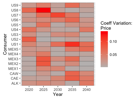
Refer to caption
(a) Coefficient of variation in Price
Refer to caption
(b) Covariance of Produced quantity
Figure 4: Covariance results
Refer to caption
(a) Price sensitivity to demand
Refer to caption
(b) Parameter sensitivity comparison
Figure 5: Sensitivity results

Fig. 5 shows the sensitivity of the solution to various input parameters. The graph on Fig. 5(a) shows the sum total change in uncertainty in price for a 1% fluctuation in the demand curve of consumers. We notice that the price is particularly sensitive to changes in demand in Mexico. This reflects the increasing concern about growing exports (both LNG and pipeline) that are likely to result in higher consumer prices in the U.S. We also note that fluctuations in demand at nodes where production facilities are not available (MEX1, MEX3, MEX4) cause greater uncertainty in price. This is because, for regions with a production facility in the same node, the production facility produces more to cater the demand at that node and there is little effect in the flows and in the prices at other nodes. This is also contingent to sufficient pipeline capacity. Larger changes in demand for regions with limited pupeline capacity (e.g. MEX1) may result in major changes in price. However a perturbation to the demand at a node with no production unit causes the flows to alter to have its demand catered. This affects natural gas availability elsewhere and causes larger fluctuations in price. The tornado plot on Fig. 5(b) sorts the parameters in decreasing order of their effect on the uncertainty of the solution.

The plot Fig. 5(b) shows the total change of the equilibrium if a parameter (e.g., the demand intercept) is shifted by 1% from its original value. Note that the results are plotted in logarithmic scale and are sorted in decreasing order. In general, our results suggest that parameters of consumers and producers play a major role on the equilibrium and hence a small perturbation have a large effect on the solution. In particular, the intercept and slope of the demand curve and the linear cost parameter are the three most significant parameters. Interestingly, the expansion cost parameters (pipeline as well as production expansion) have a lower effect on the solution equilibrium. As it was described on Fig 5(a), uncertainties in demand significantly affect regions with no or low production capacities. Fig 5(b) corroborates that changes to the demand affects the equilibrium the most. The results also indicate that the infrastructure expansion happens independently of changes in expansion cost. Natural gas prices paid by consumers account for cost expansions and transportation. Therefore, the level of expansion is then driven by changes on demand. Hence, if policy changes need to be implemented in order to, for instance, to increase economic activity or reduce carbon emissions, respectively subsidizes or taxes the downstream or upstream ends of market rather than the mid-stream players to have larger impacts. However, a policy maker who is interested in generating revenue without much impacts on the equilibrium should tax fuel transportation or infrastructure expansion for the greatest benefit.

7 Conclusion and Future work

In this paper, we developed a method to approximate the covariance of the output of a large-scale nonlinear complementarity problem with random input parameters using first-order approximation methods. We extended this method to general optimization problems with equality constraints. We then developed sensitivity metrics for each of the input parameters quantifying their contribution to the uncertainty in the output. We used these tools to understand the covariance in the equilibrium of the North American natural gas Market. The method gave insights into how production, consumption, pipeline flows, prices would vary due to large uncertainties. While the variances identified the regions that are affected the most, the covariance gave information about whether the quantity will increase or decrease due to perturbation in the input. We also obtained results on the sensitivity of price uncertainty to demand uncertainty in various nodes. We then quantified the contribution of each input parameter to the uncertainty in the output. This in turn, helps in identifying the regions that can have large impacts on equilibrium.

We note that the method is particularly useful for large-scale nonlinear complementarity problems with a large number of uncertain parameters, which make Monte-Carlo simulations intractable. It is robust in approximating the solution covariance for small uncertainty in the inputs. It is also good in quantifying the sensitivity of the output (and its variance) to the variance of input parameters. However since all the above are obtained as an approximation based on first-order metrics, there is a compromise in the accuracy if the variances of the input are large. The method works the best for problems involving a large number of decision variables and random parameters with small variance.

We foresee expanding this work by using progressively higher order terms of the Taylor series to capture the nonlinearities more efficiently. To ensure computational feasibility, this would typically require us to have stronger assumptions on the sparsity of the Hessian and the higher-order derivatives. This will also require analysis and stronger assumptions about higher-order moments of the random parameters.

8 Acknowledgements

The model in this article is based in part on the multi-fuel energy equilibrium model MultiMod Huppmann and Egging [2014]. The MultiMod was developed by Dr. Daniel Huppmann at DIW Berlin as part of the RESOURCES project, in collaboration with Dr. Ruud Egging (NTNU, Trondheim), Dr. Franziska Holz (DIW Berlin) and others (see http://diw.de/multimod). We are grateful to the original developers of MultiMod for sharing the mathematical implementation, which we further extended as part of this work.

The authors would also like to thank Dr. Donniell Fishkind, Department of Applied Mathematics and Statistics, Johns Hopkins University, Dr. Michael Ferris, Department of Computer Sciences, University of Wisconsin-Madison and the participants of TAI conference 2016, MOPTA 2016 and INFORMS 2016 for their valuable comments and discussions.

The authors would also like to thank the two anonymous reviewers whose comments and suggestions improved this paper.

9 Proofs to certain lemmas and propositions

Proof of Lemma 3.

To show this, we first prove that every element in 𝕂′\mathbb{K}^{\prime} indeed is in 𝕂∗\mathbb{K}^{*}. And then we prove for every element 𝐱∉𝕂′{\mathbf{x}}\not\in\mathbb{K}^{\prime}, there exists some 𝐯∈𝕂\mathbf{v}\in\mathbb{K} such that 𝐯T​𝐱<0\mathbf{v}^{T}{\mathbf{x}}<0.
Consider an arbitrary 𝐱{\mathbf{x}} in 𝕂′\mathbb{K}^{\prime}.

𝐯T​𝐱=∑i=1n𝐯i​𝐱i=∑i∈ℐ𝐯i​𝐱i+∑i∉ℐ𝐯i​𝐱i≥0\displaystyle\mathbf{v}^{T}{\mathbf{x}}\quad=\quad\sum_{i=1}^{n}\mathbf{v}_{i}{\mathbf{x}}_{i}\quad=\quad\sum_{i\in\mathcal{I}}\mathbf{v}_{i}{\mathbf{x}}_{i}+\sum_{i\not\in\mathcal{I}}\mathbf{v}_{i}{\mathbf{x}}_{i}\quad\geq\quad 0 (9.1)

where the final inequality follows from the fact that each term in the first summation is individually non-negative and each term in the second summation is 0. Thus we have 𝕂′⊆𝕂∗\mathbb{K}^{\prime}\subseteq\mathbb{K}^{*}.
Now to show the reverse containment, suppose there is 𝐱∈ℝn;𝐱∉𝕂′{\mathbf{x}}\in\mathbb{R}^{n};{\mathbf{x}}\not\in\mathbb{K}^{\prime}. This means, we either have

  1. 1.

    at least one index j∈ℐj\in\mathcal{I} such that 𝐱j<0{\mathbf{x}}_{j}<0 or

  2. 2.

    at least one index j∉ℐj\not\in\mathcal{I} such that 𝐱j≠0{\mathbf{x}}_{j}\not=0

Now,

𝐯T​𝐱=∑i=1n𝐯i​𝐱i=𝐯j​𝐱j+∑i≠j𝐯i​𝐱i\displaystyle\mathbf{v}^{T}{\mathbf{x}}\quad=\quad\sum_{i=1}^{n}\mathbf{v}_{i}{\mathbf{x}}_{i}\quad=\quad\mathbf{v}_{j}{\mathbf{x}}_{j}+\sum_{i\not=j}\mathbf{v}_{i}{\mathbf{x}}_{i} (9.2)

In the first case, choose 𝐯\mathbf{v} such that [𝐯]i=0[\mathbf{v}]_{i}=0 for i≠ji\not=j and 𝐯j=1\mathbf{v}_{j}=1. Clearly 𝐯∈𝕂\mathbf{v}\in\mathbb{K} and for this choice of 𝐯\mathbf{v}, the above sum is negative, showing 𝐱∉𝕂∗{\mathbf{x}}\not\in\mathbb{K}^{*}. In the second case, choose 𝐯\mathbf{v} such that [𝐯]i=0[\mathbf{v}]_{i}=0 for i≠ji\not=j and 𝐯j=−sgn(𝐱j)\mathbf{v}_{j}=-\sgn({\mathbf{x}}_{j}). Clearly 𝐯∈𝕂\mathbf{v}\in\mathbb{K} and for this choice of 𝐯\mathbf{v}, the above sum is negative, showing 𝐱∉𝕂∗{\mathbf{x}}\not\in\mathbb{K}^{*}. Thus we show (𝕂′)c⊆(𝕂∗)c\left(\mathbb{K}^{\prime}\right)^{c}\subseteq\left(\mathbb{K}^{*}\right)^{c}, which implies the reverse containment and completes the proof. ∎

Proof of Proposition 5.

Since 𝐱∗≡𝐱∗​(θ){\color[rgb]{0,0,0}{\mathbf{x}}^{*}}\equiv{\color[rgb]{0,0,0}{\mathbf{x}}^{*}}({\mathbf{{\theta}}}) solves the problem, following from the requirement that 𝐅⁡(𝐱∗)∈𝕂∗{\color[rgb]{0,0,0}\mathbf{{\color[rgb]{0,0,0}\mathbf{F}}}}({\color[rgb]{0,0,0}{\mathbf{x}}^{*}})\in\mathbb{K}^{*} and lemma 3, if i∉ℐi\not\in\mathcal{I}, 𝐅i​(𝐱∗,θ)=0{\color[rgb]{0,0,0}\mathbf{F}}_{i}({\color[rgb]{0,0,0}{\mathbf{x}}^{*}};{\mathbf{{\theta}}})=0.
For i∈ℐi\in\mathcal{I}, 𝐱∗∈𝕂⇒𝐱∗i≥0{\color[rgb]{0,0,0}{\mathbf{x}}^{*}}\in\mathbb{K}\Rightarrow{\color[rgb]{0,0,0}{\mathbf{x}}^{*}}_{i}\geq 0 and 𝐅⁡(𝐱∗)∈𝕂∗⇒𝐅i​(𝐱∗)≥0{\color[rgb]{0,0,0}\mathbf{{\color[rgb]{0,0,0}\mathbf{F}}}}({\color[rgb]{0,0,0}{\mathbf{x}}^{*}})\in\mathbb{K}^{*}\Rightarrow{\color[rgb]{0,0,0}\mathbf{F}}_{i}({\color[rgb]{0,0,0}{\mathbf{x}}^{*}})\geq 0. Also from the requirement 𝐱∗T​𝐅​(𝐱∗)=0{\color[rgb]{0,0,0}{\mathbf{x}}^{*}}^{T}{\color[rgb]{0,0,0}\mathbf{{\color[rgb]{0,0,0}\mathbf{F}}}}({\color[rgb]{0,0,0}{\mathbf{x}}^{*}})=0, one of the above two quantities should vanish for each i∈ℐi\in\mathcal{I}. But C-functions are precisely functions that vanish when both their arguments are non-negative and of them equal zero. So ψi​(𝐱∗,𝐅i​(𝐱∗))=0{\color[rgb]{0,0,0}\psi}_{i}({\color[rgb]{0,0,0}{\mathbf{x}}^{*}},{\color[rgb]{0,0,0}\mathbf{F}}_{i}({\color[rgb]{0,0,0}{\mathbf{x}}^{*}}))=0.
Thus each coordinate of Φ{\color[rgb]{0,0,0}\Phi} is individually zero, which makes 𝖿⁡(𝐱∗){\color[rgb]{0,0,0}\mathsf{f}}({\color[rgb]{0,0,0}{\mathbf{x}}^{*}}) vanish, which is the smallest value 𝖿{\color[rgb]{0,0,0}\mathsf{f}} can take. Thus 𝐱∗{\color[rgb]{0,0,0}{\mathbf{x}}^{*}} is a global minimum of 𝖿{\color[rgb]{0,0,0}\mathsf{f}}. ∎

Proof of Proposition 6.

Since a solution exists for the NCP, we know by proposition 5 that the minimum value 𝖿{\color[rgb]{0,0,0}\mathsf{f}} can take is 0. Suppose we have 𝐱∗∈ℝn{\color[rgb]{0,0,0}{\mathbf{x}}^{*}}\in\mathbb{R}^{n} such that 𝖿⁡(𝐱∗,θ)=0{\color[rgb]{0,0,0}\mathsf{f}}({\color[rgb]{0,0,0}{\mathbf{x}}^{*}};{\mathbf{{\theta}}})=0. Since 𝖿{\color[rgb]{0,0,0}\mathsf{f}} is sum of squares, this can happen only if each of the individual terms are zero. This means for i∉ℐi\not\in\mathcal{I}, 𝐅i​(𝐱∗)=0{\color[rgb]{0,0,0}\mathbf{F}}_{i}({\color[rgb]{0,0,0}{\mathbf{x}}^{*}})=0.
Now since ψi​(𝐱i,𝐅i​(𝐱∗))=0{\color[rgb]{0,0,0}\psi}_{i}({\mathbf{x}}_{i},{\color[rgb]{0,0,0}\mathbf{F}}_{i}({\color[rgb]{0,0,0}{\mathbf{x}}^{*}}))=0 for i∈ℐi\in\mathcal{I}, we know 𝐅i​(𝐱∗)≥0{\color[rgb]{0,0,0}\mathbf{F}}_{i}({\color[rgb]{0,0,0}{\mathbf{x}}^{*}})\geq 0. This combined with the previous point implies 𝐅⁡(𝐱∗)∈𝕂∗{\color[rgb]{0,0,0}\mathbf{{\color[rgb]{0,0,0}\mathbf{F}}}}({\color[rgb]{0,0,0}{\mathbf{x}}^{*}})\in\mathbb{K}^{*}.
Also from the fact that ψi​(𝐱∗i,𝐅i​(𝐱∗,θ))=0{\color[rgb]{0,0,0}\psi}_{i}({\color[rgb]{0,0,0}{\mathbf{x}}^{*}}_{i};{\color[rgb]{0,0,0}\mathbf{F}}_{i}({\color[rgb]{0,0,0}{\mathbf{x}}^{*}};{\mathbf{{\theta}}}))=0 for i∈ℐi\in\mathcal{I}, we know that 𝐱∗∈𝕂{\color[rgb]{0,0,0}{\mathbf{x}}^{*}}\in\mathbb{K}. It also implies that 𝐱∗i​𝐅i​(𝐱∗)=0{\color[rgb]{0,0,0}{\mathbf{x}}^{*}}_{i}{\color[rgb]{0,0,0}\mathbf{F}}_{i}({\color[rgb]{0,0,0}{\mathbf{x}}^{*}})=0 for i∈ℐi\in\mathcal{I}. Thus

𝐱∗T​𝐅​(𝐱∗,θ)\displaystyle{\color[rgb]{0,0,0}{\mathbf{x}}^{*}}^{T}{\color[rgb]{0,0,0}\mathbf{{\color[rgb]{0,0,0}\mathbf{F}}}}({\color[rgb]{0,0,0}{\mathbf{x}}^{*}};{\mathbf{{\theta}}})\quad =∑i=1n𝐱∗i​𝐅i\displaystyle=\quad\sum_{i=1}^{n}{\color[rgb]{0,0,0}{\mathbf{x}}^{*}}_{i}{\color[rgb]{0,0,0}\mathbf{F}}_{i} (9.3)
=∑i∈ℐ𝐱∗i​𝐅i+∑i∉ℐ𝐱∗i​𝐅i\displaystyle=\quad\sum_{i\in\mathcal{I}}{\color[rgb]{0,0,0}{\mathbf{x}}^{*}}_{i}{\color[rgb]{0,0,0}\mathbf{F}}_{i}+\sum_{i\not\in\mathcal{I}}{\color[rgb]{0,0,0}{\mathbf{x}}^{*}}_{i}{\color[rgb]{0,0,0}\mathbf{F}}_{i} (9.4)
=0+0=0\displaystyle=\quad 0+0\quad=\quad 0 (9.5)

This implies 𝐱∗​(θ)⟂𝐅⁡(𝐱∗,θ){\color[rgb]{0,0,0}{\mathbf{x}}^{*}}({\mathbf{{\theta}}})\perp{\color[rgb]{0,0,0}\mathbf{{\color[rgb]{0,0,0}\mathbf{F}}}}({\color[rgb]{0,0,0}{\mathbf{x}}^{*}};{\mathbf{{\theta}}}) and 𝐱∗​(θ){\color[rgb]{0,0,0}{\mathbf{x}}^{*}}({\mathbf{{\theta}}}) solves the complementarity problem. ∎

Proof of Corollary 8.

The set O={(a,b):ψm​i​n​(a,b)=0}∖{(0,0)}O=\left\{(a,b):{\color[rgb]{0,0,0}\psi}_{min}(a,b)=0\right\}\setminus\left\{(0,0)\right\} is the positive coordinate axes except the origin. Rewriting this C-function as

ψm​i​n​(a,b)\displaystyle{\color[rgb]{0,0,0}\psi}_{min}(a,b)\quad ={a if ​a<bb otherwise\displaystyle=\quad\left\{\begin{array}[]{ll}a&\mbox{ if }a<b\\ b&\mbox{ otherwise}\end{array}\right.

we see that the second derivative of ψm​i​n{\color[rgb]{0,0,0}\psi}_{min} vanishes at OO. Also we observe that

lim(a,b)→(0,0)ψ2​(a,b)​∂2ψ⁡(a,b)∂a​∂b\displaystyle\lim_{(a,b)\rightarrow(0,0)}{\color[rgb]{0,0,0}\psi}^{2}(a,b)\frac{\partial^{2}{\color[rgb]{0,0,0}\psi}(a,b)}{\partial a\partial b}\quad =0\displaystyle=\quad 0 (9.8)

since the second derivative is 0 everywhere except along the line a=ba=b. ∎

Proof of Corollary 9.

For ψ=ψF​B{\color[rgb]{0,0,0}\psi}={\color[rgb]{0,0,0}\psi}_{FB}, we have assumption 1 of proposition 7 satisfied by Facchinei and Pang [2007]. For assumption 2,

lim(a,b)→(0,0)ψ2​(a,b)​∂2ψ⁡(a,b)∂a​∂b\displaystyle\lim_{(a,b)\rightarrow(0,0)}{\color[rgb]{0,0,0}\psi}^{2}(a,b)\frac{\partial^{2}{\color[rgb]{0,0,0}\psi}(a,b)}{\partial a\partial b}\quad =lim(a,b)→(0,0)(a2+b2−a−b)2​a​b(a2+b2)3\displaystyle=\quad\lim_{(a,b)\rightarrow(0,0)}\left(\sqrt{a^{2}+b^{2}}-a-b\right)^{2}\frac{ab}{\left(\sqrt{a^{2}+b^{2}}\right)^{3}} (9.9)
=0\displaystyle=\quad 0 (9.10)

Thus 𝖿{\color[rgb]{0,0,0}\mathsf{f}} is twice continuously differentiable at its zeros. The twice continuous differentiability elsewhere follows directly from the fact that ψF​B{\color[rgb]{0,0,0}\psi}_{FB} is twice continuously differentiable everywhere except at the origin. This ensures that all the terms in the derivative of the sum of squares exist and are finite. ∎

Proof of Proposition 14.

By definition, for some admissible dd,

𝖿⁡(𝐱+δ​ed)\displaystyle{\color[rgb]{0,0,0}\mathsf{f}}({\mathbf{x}}+\delta e_{d})\quad =𝖿⁡(𝐱)+δ​G​ed+o⁡(δ2)\displaystyle=\quad{\color[rgb]{0,0,0}\mathsf{f}}({\mathbf{x}})+\delta Ge_{d}+o(\delta^{2}) (9.11)
⇒[𝖿⁡(𝐱+δ​ed)]i\displaystyle\Rightarrow[{\color[rgb]{0,0,0}\mathsf{f}}({\mathbf{x}}+\delta e_{d})]_{i}\quad =[𝖿⁡(𝐱)]i+δ​Gi​d+o⁡(δ2)\displaystyle=\quad[{\color[rgb]{0,0,0}\mathsf{f}}({\mathbf{x}})]_{i}+\delta G_{id}+o(\delta^{2}) (9.12)
‖𝖿⁡(𝐱+δ​ed)‖2\displaystyle\|{\color[rgb]{0,0,0}\mathsf{f}}({\mathbf{x}}+\delta e_{d})\|_{2}\quad ≤∥𝖿(𝐱)∥2+∥δG.d∥2+∥o(δ2)∥2\displaystyle\leq\quad\|{\color[rgb]{0,0,0}\mathsf{f}}({\mathbf{x}})\|_{2}+\|\delta G_{.d}\|_{2}+\|o(\delta^{2})\|_{2} (9.13)
=‖𝖿⁡(𝐱)‖2+δ​(∑i=1nGi​d2)+o⁡(δ2)\displaystyle=\quad\|{\color[rgb]{0,0,0}\mathsf{f}}({\mathbf{x}})\|_{2}+\delta\sqrt{\left(\sum_{i=1}^{n}G_{id}^{2}\right)}+o(\delta^{2}) (9.14)

where G.dG_{.d} is the dd-th column of GG. Also we have from (9.12) for sufficiently small δ\delta,

‖𝖿⁡(𝐱+δ​ed)‖2\displaystyle\|{\color[rgb]{0,0,0}\mathsf{f}}({\mathbf{x}}+\delta e_{d})\|_{2}\quad ≥∥𝖿(𝐱)∥2−∥δG.d∥2+∥o(δ2)∥2\displaystyle\geq\quad\|{\color[rgb]{0,0,0}\mathsf{f}}({\mathbf{x}})\|_{2}-\|\delta G_{.d}\|_{2}+\|o(\delta^{2})\|_{2} (9.15)
=‖𝖿⁡(𝐱)‖2−δ​(∑i=1nGi​d2)+o⁡(δ2)\displaystyle=\quad\|{\color[rgb]{0,0,0}\mathsf{f}}({\mathbf{x}})\|_{2}-\delta\sqrt{\left(\sum_{i=1}^{n}G_{id}^{2}\right)}+o(\delta^{2}) (9.16)

∎

Proof of Corollary 17.

For the problem to be well-defined, let G∈ℝn×nG\in\mathbb{R}^{n\times n} and θ∈ℝn{\mathbf{{\theta}}}\in\mathbb{R}^{n}. This makes ∇𝐱​θ2​𝖿​(𝐱,θ)∈ℝn×n\nabla^{2}_{{\mathbf{x}}{\mathbf{{\theta}}}}{\color[rgb]{0,0,0}\mathsf{f}}({\mathbf{x}};{\mathbf{{\theta}}})\in\mathbb{R}^{n\times n}.

∇𝐱𝖿​(𝐱,θ)\displaystyle{\color[rgb]{0,0,0}\nabla_{{\mathbf{x}}}{\color[rgb]{0,0,0}\mathsf{f}}}({\mathbf{x}};{\mathbf{{\theta}}})\quad =G​𝐱+θ⁡(ω)\displaystyle=\quad G{\mathbf{x}}+{\mathbf{{\theta}}}({\color[rgb]{0,0,0}\omega}) (9.17)
∇𝐱2​𝖿​(𝐱,θ)\displaystyle{\color[rgb]{0,0,0}\nabla_{{\mathbf{x}}}^{2}{\color[rgb]{0,0,0}\mathsf{f}}}({\mathbf{x}};{\mathbf{{\theta}}})\quad =G\displaystyle=\quad G (9.18)
[∇𝐱​θ2​𝖿​(𝐱,θ)]i​j\displaystyle[\nabla^{2}_{{\mathbf{x}}{\mathbf{{\theta}}}}{\color[rgb]{0,0,0}\mathsf{f}}({\mathbf{x}};{\mathbf{{\theta}}})]_{ij}\quad =I\displaystyle=\quad I (9.19)

Due to absence of terms dependent on 𝐱{\mathbf{x}} in the last two equations, we have an exact equation,

G​Δ​𝐱\displaystyle G\Delta{\mathbf{x}}\quad =Δ​θ\displaystyle=\quad{\color[rgb]{0,0,0}\Delta{\mathbf{{\theta}}}} (9.20)

Due to the exactness of the above equation, we have

𝒯\displaystyle{\color[rgb]{0,0,0}\mathcal{T}}\quad =G−1\displaystyle=\quad G^{-1} (9.21)
𝒞​ov⁡(Δ​𝐱)\displaystyle\cov(\Delta{\mathbf{x}})\quad =𝒯𝒞​ov(Δθ)𝒯T\displaystyle=\quad{\color[rgb]{0,0,0}\mathcal{T}}\cov({\color[rgb]{0,0,0}\Delta{\mathbf{{\theta}}}}){\color[rgb]{0,0,0}\mathcal{T}}^{T} (9.22)

with no error. ∎

10 Natural Gas Market - Complementarity Formulation

In this formulation, we assume we have a set of suppliers P, consumers C and a pipeline operator. The players are located in a set of nodes N, and some of them are connected by pipelines A.
Let also say that Pn⊆P{\text{P}}_{n}\subseteq{\text{P}}, Cn⊆C{\text{C}}_{n}\subseteq{\text{C}} are located in node n∈Nn\in{\text{N}}. Let An{\text{A}}_{n} be the pipelines connected to node nn. The symbols used here are explained in Table 1, 2 and 3. Most of the analysis closely follow Feijoo et al. [2016] and Egging et al. [2016]. Random parameters are denoted by an (ω)({\color[rgb]{0,0,0}\omega}) beside them. The implementation of this problem is made available in https://github.com/ssriram1992/Stoch_Aprx_cov.

Refer to caption
Refer to caption
Figure 6: Regional disaggregation of United States and Mexico. Source: AEO [2015] and U.S. Energy Information Administration http://www.eia.gov/todayinenergy/detail.php?id=16471

10.1 Producer’s problem

Maximize∑Y𝖽𝖿y(ω)\displaystyle\Max\sum_{{\text{Y}}}{\color[rgb]{0,0,0}\mathsf{df}_{y}({\color[rgb]{0,0,0}\omega})} {∑CQp​c​n​yCπ𝐜𝐲−Gol(Qp​n​yP,CAPp​yP)\displaystyle\left\{\sum_{{\text{C}}}{\color[rgb]{0,0,0}{\text{Q}}_{pcny}^{{\text{C}}}}{\color[rgb]{0,0,0}\mathbf{{\mathbf{\pi}}_{cy}}}-{\color[rgb]{0,0,0}\mbox{Gol}}\left({\color[rgb]{0,0,0}{\text{Q}}_{pny}^{{\text{P}}}},{\color[rgb]{0,0,0}\text{CAP}^{{\text{P}}}_{py}}\right)\right.
−πp​yXP(ω)Xp​yP−∑An+π𝐚𝐲AQp​a​yA}\displaystyle\left.\quad-{\color[rgb]{0,0,0}{\mathbf{\pi}}^{{\text{X}}{\text{P}}}_{py}({\color[rgb]{0,0,0}\omega})}{\color[rgb]{0,0,0}{\text{X}}^{{\text{P}}}_{p{y}}}-\sum_{{{\text{A}}_{n}^{+}}}{\color[rgb]{0,0,0}\mathbf{{\mathbf{\pi}}^{{\text{A}}}_{ay}}}{\color[rgb]{0,0,0}{\text{Q}}_{pay}^{{\text{A}}}}\right\} (10.1)

subject to

Qp​c​n​yC,Qp​n​yP,Qp​a​yA\displaystyle{\color[rgb]{0,0,0}{\text{Q}}_{pcny}^{{\text{C}}}},{\color[rgb]{0,0,0}{\text{Q}}_{pny}^{{\text{P}}}},{\color[rgb]{0,0,0}{\text{Q}}_{pay}^{{\text{A}}}}\quad ≥0\displaystyle\geq\quad 0
Xp​yP,CAPp​yP\displaystyle{\color[rgb]{0,0,0}{\text{X}}^{{\text{P}}}_{p{y}}},{\color[rgb]{0,0,0}\text{CAP}^{{\text{P}}}_{py}}\quad ≥0\displaystyle\geq\quad 0
Qp​n​yP\displaystyle{\color[rgb]{0,0,0}{\text{Q}}_{pny}^{{\text{P}}}}\quad ≤αP​CAPp​yP\displaystyle\leq\quad{\color[rgb]{0,0,0}\alpha^{{\text{P}}}}{\color[rgb]{0,0,0}\text{CAP}^{{\text{P}}}_{py}} (δp​y1)\displaystyle\left({\color[rgb]{0,0,0}\delta^{1}_{py}}\right) (10.2a)
CAPp​yP\displaystyle{\color[rgb]{0,0,0}\text{CAP}^{{\text{P}}}_{py}}\quad =Q^p​0+∑i=1yXp​iP\displaystyle=\quad{\color[rgb]{0,0,0}\hat{{\text{Q}}}_{p0}}+\sum_{i=1}^{y}{\color[rgb]{0,0,0}{\text{X}}^{{\text{P}}}_{p{i}}} (δp​y2)\displaystyle\left({\color[rgb]{0,0,0}\delta^{2}_{p{y}}}\right) (10.2b)
∑CnQp​c​n​yC+∑An+Qp​a​yA\displaystyle\sum_{{\text{C}}_{n}}{\color[rgb]{0,0,0}{\text{Q}}_{pcny}^{{\text{C}}}}+\sum_{{{\text{A}}_{n}^{+}}}{\color[rgb]{0,0,0}{\text{Q}}_{pay}^{{\text{A}}}}\quad =Qp​n​yP​(1−Lp​yP​(ω))\displaystyle=\quad{\color[rgb]{0,0,0}{\text{Q}}_{pny}^{{\text{P}}}}(1-{\color[rgb]{0,0,0}{\color[rgb]{0,0,0}L}^{{\text{P}}}_{py}({\color[rgb]{0,0,0}\omega})})
+∑An−Qp​a​yA(1−La​yA(ω))\displaystyle\quad\qquad+\sum_{{{\text{A}}_{n}^{-}}}{\color[rgb]{0,0,0}{\text{Q}}_{pay}^{{\text{A}}}}(1-{\color[rgb]{0,0,0}{\color[rgb]{0,0,0}L}^{{\text{A}}}_{ay}({\color[rgb]{0,0,0}\omega})}) (δp​n​y3)\displaystyle\left({\color[rgb]{0,0,0}\delta^{3}_{pny}}\right) (10.2c)

where

Gol(.)\displaystyle{\color[rgb]{0,0,0}\mbox{Gol}}(.)\quad =(lp​yP​(ω)+gp​yP​(ω))​Qp​n​yP+qp​yP​(ω)​Qp​n​yP2\displaystyle=\quad({\color[rgb]{0,0,0}l^{{\text{P}}}_{py}({\color[rgb]{0,0,0}\omega})}+{\color[rgb]{0,0,0}g^{{\text{P}}}_{py}({\color[rgb]{0,0,0}\omega})}){\color[rgb]{0,0,0}{\text{Q}}_{pny}^{{\text{P}}}}+{\color[rgb]{0,0,0}q^{{\text{P}}}_{py}({\color[rgb]{0,0,0}\omega})}{\color[rgb]{0,0,0}{\text{Q}}_{pny}^{{\text{P}}}}^{2}
+gp​yP​(ω)​(CAPp​yP−Qp​n​yP)​log⁡(1−Qp​n​yPCAPp​yP)\displaystyle\quad\qquad+{\color[rgb]{0,0,0}g^{{\text{P}}}_{py}({\color[rgb]{0,0,0}\omega})}({\color[rgb]{0,0,0}\text{CAP}^{{\text{P}}}_{py}}-{\color[rgb]{0,0,0}{\text{Q}}_{pny}^{{\text{P}}}})\log\left(1-\frac{{\color[rgb]{0,0,0}{\text{Q}}_{pny}^{{\text{P}}}}}{{\color[rgb]{0,0,0}\text{CAP}^{{\text{P}}}_{py}}}\right) (10.3)
Table 1: Sets
Set Explanation Set Explanation
P Set of suppliers A Set of pipeline connections(arcs)
C Set of consumers An+{{\text{A}}_{n}^{+}} Set of arcs from node nn on which natural gas flows out
N Set of nodes An−{{\text{A}}_{n}^{-}} Set of arcs from node nn on which natural gas flows in
Y Set of periods
Table 2: Symbols - Variables
Symbol Explanation
Quantities Qp​c​n​yC{\color[rgb]{0,0,0}{\text{Q}}_{pcny}^{{\text{C}}}} Quantity produced by pp in nn to send to cc in year yy
Qp​n​yP{\color[rgb]{0,0,0}{\text{Q}}_{pny}^{{\text{P}}}} Total quantity produced by pp in year yy
Qp​a​yA{\color[rgb]{0,0,0}{\text{Q}}_{pay}^{{\text{A}}}} Total quantity pp choses to send by arc aa in year yy
Qa​yA{\color[rgb]{0,0,0}{\text{Q}}_{ay}^{{\text{A}}}} Total quantity sent by aa during year yy
Prices π𝐜𝐲{\color[rgb]{0,0,0}\mathbf{{\mathbf{\pi}}_{cy}}} Unit price paid by consumer CC in year YY
π𝐚𝐲A{\color[rgb]{0,0,0}\mathbf{{\mathbf{\pi}}^{{\text{A}}}_{ay}}} Unit price of sending natural gas through aa during year yy
Capacity Xp​yP{\color[rgb]{0,0,0}{\text{X}}^{{\text{P}}}_{p{y}}} Production expansion in year yy for supplier pp
Xa​yA{\color[rgb]{0,0,0}{\text{X}}^{{\text{A}}}_{a{y}}} Transportation capacity expansion in year yy for arc aa
CAPp​yP{\color[rgb]{0,0,0}\text{CAP}^{{\text{P}}}_{py}} Production capacity for supplier pp in year yy
CAPa​yA{\color[rgb]{0,0,0}\text{CAP}^{{\text{A}}}_{ay}} Transportation capacity for arc aa in year yy
Table 3: Symbols - Parameters
Symbol Explanation
Quantities Q^p​0{\color[rgb]{0,0,0}\hat{{\text{Q}}}_{p0}} Initial capacity of production for supplier pp
Q^a​0{\color[rgb]{0,0,0}\hat{{\text{Q}}}_{a0}} Initial capacity of transportation for pipeline aa
Prices πp​yXP​(ω){\color[rgb]{0,0,0}{\mathbf{\pi}}^{{\text{X}}{\text{P}}}_{py}({\color[rgb]{0,0,0}\omega})} Price of capacity expansion for supplier pp
πa​yXA​(ω){\color[rgb]{0,0,0}{\mathbf{\pi}}^{{\text{X}}{\text{A}}}_{ay}({\color[rgb]{0,0,0}\omega})} Price of capacity expansion for transportation arc aa
Losses Lp​yP​(ω){\color[rgb]{0,0,0}{\color[rgb]{0,0,0}L}^{{\text{P}}}_{py}({\color[rgb]{0,0,0}\omega})} Percentage loss in production by supplier pp in year yy
La​yA​(ω){\color[rgb]{0,0,0}{\color[rgb]{0,0,0}L}^{{\text{A}}}_{ay}({\color[rgb]{0,0,0}\omega})} Percentage loss in transportation via arc aa in year yy
αP{\color[rgb]{0,0,0}\alpha^{{\text{P}}}} Availability fraction of the production capacity
Consumer Ec​yC​(ω){\color[rgb]{0,0,0}E^{{\text{C}}}_{cy}({\color[rgb]{0,0,0}\omega})} Intercept of the demand curve for consumer cc in year yy
Dc​yC​(ω){\color[rgb]{0,0,0}D^{{\text{C}}}_{cy}({\color[rgb]{0,0,0}\omega})} Slope of the demand curve for consumer cc in year yy
𝖽𝖿y​(ω){\color[rgb]{0,0,0}\mathsf{df}_{y}({\color[rgb]{0,0,0}\omega})} Discount Factor for year yy

10.2 Pipeline operator’s problem

Maximize∑Y\displaystyle\Max\sum_{{\text{Y}}} 𝖽𝖿y​(ω)​{∑AQa​yA​(π𝐚𝐲A−γy​aA​(ω))−πa​yXA​(ω)​Xa​yA}\displaystyle{\color[rgb]{0,0,0}\mathsf{df}_{y}({\color[rgb]{0,0,0}\omega})}\left\{\sum_{{\text{A}}}{\color[rgb]{0,0,0}{\text{Q}}_{ay}^{{\text{A}}}}\left({\color[rgb]{0,0,0}\mathbf{{\mathbf{\pi}}^{{\text{A}}}_{ay}}}-{\color[rgb]{0,0,0}\gamma_{ya}^{{\text{A}}}({\color[rgb]{0,0,0}\omega})}\right)-{\color[rgb]{0,0,0}{\mathbf{\pi}}^{{\text{X}}{\text{A}}}_{ay}({\color[rgb]{0,0,0}\omega})}{\color[rgb]{0,0,0}{\text{X}}^{{\text{A}}}_{a{y}}}\right\} (10.4)

subject to

Qa​yA,Xa​yA,CAPa​yA\displaystyle{\color[rgb]{0,0,0}{\text{Q}}_{ay}^{{\text{A}}}},{\color[rgb]{0,0,0}{\text{X}}^{{\text{A}}}_{a{y}}},{\color[rgb]{0,0,0}\text{CAP}^{{\text{A}}}_{ay}}\quad ≥0\displaystyle\geq\quad 0
Qa​yA\displaystyle{\color[rgb]{0,0,0}{\text{Q}}_{ay}^{{\text{A}}}}\quad ≤CAPa​yA\displaystyle\leq\quad{\color[rgb]{0,0,0}\text{CAP}^{{\text{A}}}_{ay}} (δa​y5)\displaystyle\left({\color[rgb]{0,0,0}\delta^{5}_{ay}}\right) (10.5a)
CAPa​yA\displaystyle{\color[rgb]{0,0,0}\text{CAP}^{{\text{A}}}_{ay}}\quad =Q^a​0+∑i=1yXa​iA\displaystyle=\quad{\color[rgb]{0,0,0}\hat{{\text{Q}}}_{a0}}+\sum_{i=1}^{y}{\color[rgb]{0,0,0}{\text{X}}^{{\text{A}}}_{a{i}}} (δa​y6)\displaystyle\left({\color[rgb]{0,0,0}\delta^{6}_{a{y}}}\right) (10.5b)

10.3 Consumer

π𝐜𝐲\displaystyle{\color[rgb]{0,0,0}\mathbf{{\mathbf{\pi}}_{cy}}}\quad =Ec​yC​(ω)+Dc​yC​(ω)​∑PQp​c​n​yC\displaystyle=\quad{\color[rgb]{0,0,0}E^{{\text{C}}}_{cy}({\color[rgb]{0,0,0}\omega})}+{\color[rgb]{0,0,0}D^{{\text{C}}}_{cy}({\color[rgb]{0,0,0}\omega})}\sum_{\text{P}}{\color[rgb]{0,0,0}{\text{Q}}_{pcny}^{{\text{C}}}} (π𝐜𝐲)\displaystyle\left({\color[rgb]{0,0,0}\mathbf{{\mathbf{\pi}}_{cy}}}\right) (10.6)

It can be shown that the above said optimization problems are all convex with non-empty interior. Hence the Karush-Kuhn Tucker conditions (KKT conditions) are necessary and sufficient for optimality. The KKT conditions are presented below and they form the equations for the complementarity problem along with the constraints above.

10.4 KKT to Producer’s problem

−𝖽𝖿y​(ω)​π𝐜𝐲+δp​n​y3\displaystyle-{\color[rgb]{0,0,0}\mathsf{df}_{y}({\color[rgb]{0,0,0}\omega})}{\color[rgb]{0,0,0}\mathbf{{\mathbf{\pi}}_{cy}}}+{\color[rgb]{0,0,0}\delta^{3}_{pny}}\quad ≥0\displaystyle\geq\quad 0 (Qp​c​n​yC)\displaystyle\left({\color[rgb]{0,0,0}{\text{Q}}_{pcny}^{{\text{C}}}}\right) (10.7a)
𝖽𝖿y​(ω)​πp​yXP​(ω)−∑i=1yδp​i2\displaystyle{\color[rgb]{0,0,0}\mathsf{df}_{y}({\color[rgb]{0,0,0}\omega})}{\color[rgb]{0,0,0}{\mathbf{\pi}}^{{\text{X}}{\text{P}}}_{py}({\color[rgb]{0,0,0}\omega})}-\sum_{i=1}^{y}{\color[rgb]{0,0,0}\delta^{2}_{p{i}}}\quad ≥0\displaystyle\geq\quad 0 (Xp​yP)\displaystyle\left({\color[rgb]{0,0,0}{\text{X}}^{{\text{P}}}_{p{y}}}\right) (10.7b)
𝖽𝖿y​(ω)​π𝐚𝐲A+(𝕀a∈An+−𝕀a∈An−​(1−La​yA​(ω)))​δp​n​y3\displaystyle{\color[rgb]{0,0,0}\mathsf{df}_{y}({\color[rgb]{0,0,0}\omega})}{\color[rgb]{0,0,0}\mathbf{{\mathbf{\pi}}^{{\text{A}}}_{ay}}}+\left(\mathbb{I}_{a\in{{\text{A}}_{n}^{+}}}-\mathbb{I}_{a\in{{\text{A}}_{n}^{-}}}(1-{\color[rgb]{0,0,0}{\color[rgb]{0,0,0}L}^{{\text{A}}}_{ay}({\color[rgb]{0,0,0}\omega})})\right){\color[rgb]{0,0,0}\delta^{3}_{pny}}\quad ≥0\displaystyle\geq\quad 0 (Qp​a​yA)\displaystyle\left({\color[rgb]{0,0,0}{\text{Q}}_{pay}^{{\text{A}}}}\right) (10.7c)
𝖽𝖿y​(ω)​∂Gol∂Qp​n​yP+δp​y1−δp​n​y3​(1−Lp​yP​(ω))\displaystyle{\color[rgb]{0,0,0}\mathsf{df}_{y}({\color[rgb]{0,0,0}\omega})}\frac{\partial{\color[rgb]{0,0,0}\mbox{Gol}}}{\partial{\color[rgb]{0,0,0}{\text{Q}}_{pny}^{{\text{P}}}}}+{\color[rgb]{0,0,0}\delta^{1}_{py}}-{\color[rgb]{0,0,0}\delta^{3}_{pny}}(1-{\color[rgb]{0,0,0}{\color[rgb]{0,0,0}L}^{{\text{P}}}_{py}({\color[rgb]{0,0,0}\omega})})\quad ≥0\displaystyle\geq\quad 0 (Qp​n​yP)\displaystyle\left({\color[rgb]{0,0,0}{\text{Q}}_{pny}^{{\text{P}}}}\right) (10.7d)
𝖽𝖿y​(ω)​∂Gol∂CAPp​yP+αP​δp​y2−δp​y1\displaystyle{\color[rgb]{0,0,0}\mathsf{df}_{y}({\color[rgb]{0,0,0}\omega})}\frac{\partial{\color[rgb]{0,0,0}\mbox{Gol}}}{\partial{\color[rgb]{0,0,0}\text{CAP}^{{\text{P}}}_{py}}}+{\color[rgb]{0,0,0}\alpha^{{\text{P}}}}{\color[rgb]{0,0,0}\delta^{2}_{p{y}}}-{\color[rgb]{0,0,0}\delta^{1}_{py}}\quad ≥0\displaystyle\geq\quad 0 (CAPp​yP)\displaystyle\left({\color[rgb]{0,0,0}\text{CAP}^{{\text{P}}}_{py}}\right) (10.7e)

10.5 KKT to Pipeline operator’s problem

−𝖽𝖿y​(ω)​π𝐚𝐲A+γy​aA​(ω)+δa​y5\displaystyle-{\color[rgb]{0,0,0}\mathsf{df}_{y}({\color[rgb]{0,0,0}\omega})}{\color[rgb]{0,0,0}\mathbf{{\mathbf{\pi}}^{{\text{A}}}_{ay}}}+{\color[rgb]{0,0,0}\gamma_{ya}^{{\text{A}}}({\color[rgb]{0,0,0}\omega})}+{\color[rgb]{0,0,0}\delta^{5}_{ay}}\quad ≥0\displaystyle\geq\quad 0 (Qa​yA)\displaystyle\left({\color[rgb]{0,0,0}{\text{Q}}_{ay}^{{\text{A}}}}\right) (10.8a)
𝖽𝖿y​(ω)​πa​yXA​(ω)−∑i=1yδa​i6\displaystyle{\color[rgb]{0,0,0}\mathsf{df}_{y}({\color[rgb]{0,0,0}\omega})}{\color[rgb]{0,0,0}{\mathbf{\pi}}^{{\text{X}}{\text{A}}}_{ay}({\color[rgb]{0,0,0}\omega})}-\sum_{i=1}^{y}{\color[rgb]{0,0,0}\delta^{6}_{a{i}}}\quad ≥0\displaystyle\geq\quad 0 (Xa​yA)\displaystyle\left({\color[rgb]{0,0,0}{\text{X}}^{{\text{A}}}_{a{y}}}\right) (10.8b)
δa​y6−δa​y5\displaystyle{\color[rgb]{0,0,0}\delta^{6}_{a{y}}}-{\color[rgb]{0,0,0}\delta^{5}_{ay}}\quad ≥0\displaystyle\geq\quad 0 (CAPa​yA)\displaystyle\left({\color[rgb]{0,0,0}\text{CAP}^{{\text{A}}}_{ay}}\right) (10.8c)

10.6 Market clearing condition

Qa​yA\displaystyle{\color[rgb]{0,0,0}{\text{Q}}_{ay}^{{\text{A}}}}\quad =∑PQp​a​yA\displaystyle=\quad\sum_{{\text{P}}}{\color[rgb]{0,0,0}{\text{Q}}_{pay}^{{\text{A}}}} (π𝐚𝐲A)\displaystyle({\color[rgb]{0,0,0}\mathbf{{\mathbf{\pi}}^{{\text{A}}}_{ay}}}) (10.9)

11 N-dimensional Sparse array implementation

A general purpose Python class has been implemented to handle a sparse ndarray object. The class is a generalization of the scipy class coo_matrix which stores the array coordinates of each non-zero element in the array. We now describe the details of the implementation. A continuously updated version of the class can be found at https://github.com/ssriram1992/ndsparse.

11.1 Initialization

The n-dimensional sparse array (coo_array) can be initialized by any of the following methods.

  • 1.

    A tuple, which initializes the sparse array of the shape mentioned in the tuple and with zeros everywhere.

  • 2.

    A dense ndarray which will be converted and stored as a coo_array.

  • 3.

    A matrix of positions and a 1 dimensional array of values where the matrix contains the positions of the non-zero elements and the vector containing the non-zero values of those positions. In this case the shape of the coo_array would be the smallest ndarray that can store all the elements given. Optionally a tuple containing the shape of the ndarray can be given explicitly.

  • 4.

    Another coo_array whose copy is to be created.

11.2 Methods

The following methods and attributes are available in the coo_array.

  • 1.

    print(coo_array) will result in printing the location of each of the non-zero elements of the array and their values.

  • 2.

    coo_array.flush(tol = 1e-5) will result in freeing the space used in storing any zero-elements or elements lesser than the tolerance, tol. Such numbers typically arise out arithmetic operations on coo_array or poor initialization.

  • 3.

    coo_array.size() returns the number of non-zero elements in the coo_array.

  • 4.

    coo_array.shape returns the shape of the underlying dense matrix.

  • 5.

    coo_array.add_entry(posn,val) and coo_array.set_entry(posn,val) both add a new non-zero element with the given value at the given position. The difference however is that set_entry() checks if a non-zero value already exists at the mentioned position, and if yes, overwrites it. This search makes set_entry() slower compared to add_entry() which assumes that the previous value or the position is zero. Thus add_entry() could potentially cause duplicates and ambiguity, if an illegal input is given. However in case the input is ensured to be legal, add_entry() is much faster.

  • 6.

    coo_array.get_entry(posn) returns the value at the given position.

  • 7.

    coo_array.swapaxes(axis1,axis2) is a higher dimensional generalization of matrix transposes where the dimensions that have to swapped can be chosen.

  • 8.

    coo_array.remove_duplicate_at(posn,func=0) checks if there are multiple values defined for a single position in the sparse array. If yes, they are replaced by a single entry containing the scalar valued defined by func or passes them to a function defined in func and stores the returned value. Passing a function for the argument func is incredibly useful in performing arithmetic operations on coo_array.

  • 9.

    coo_array.todense() returns a dense version of the coo_array.

  • 10.

    coo_array.iterate() returns an iterable over the non-zero positions and values in the coo_array.

The above class is used extensively to handle high-dimensional sparse arrays resulting out of variables containing pipelines, viz., Qp​a​yA,Qa​yA,Q^p​0,Q^a​0,π𝐚𝐲A,Xa​yA,δa​y5,δa​y6{\color[rgb]{0,0,0}{\text{Q}}_{pay}^{{\text{A}}}},{\color[rgb]{0,0,0}{\text{Q}}_{ay}^{{\text{A}}}},{\color[rgb]{0,0,0}\hat{{\text{Q}}}_{p0}},{\color[rgb]{0,0,0}\hat{{\text{Q}}}_{a0}},{\color[rgb]{0,0,0}\mathbf{{\mathbf{\pi}}^{{\text{A}}}_{ay}}},{\color[rgb]{0,0,0}{\text{X}}^{{\text{A}}}_{a{y}}},{\color[rgb]{0,0,0}\delta^{5}_{ay}},{\color[rgb]{0,0,0}\delta^{6}_{a{y}}} and parameters with pipelines, viz., CAPa​yA,πa​yXA​(ω),La​yA​(ω),γy​aA​(ω){\color[rgb]{0,0,0}\text{CAP}^{{\text{A}}}_{ay}},{\color[rgb]{0,0,0}{\mathbf{\pi}}^{{\text{X}}{\text{A}}}_{ay}({\color[rgb]{0,0,0}\omega})},{\color[rgb]{0,0,0}{\color[rgb]{0,0,0}L}^{{\text{A}}}_{ay}({\color[rgb]{0,0,0}\omega})},{\color[rgb]{0,0,0}\gamma_{ya}^{{\text{A}}}({\color[rgb]{0,0,0}\omega})}.

12 Computational Experiments

12.1 Problem Setup

The single-node single-product oligopoly mentioned in Section 5.1 is used for the computational experiments. Experiments were done with varying the number of players and to avoid any advantage due to symmetry, a different value was used for the cost of production for each of the nn players. The values used for the computational study are given below.

a\displaystyle a\quad =500\displaystyle=\quad 500 (12.1)
b\displaystyle b\quad =−0.5\displaystyle=\quad-0.5 (12.2)
𝔼⁡[ci]\displaystyle\mathbb{E}[c_{i}]\quad =100+3​i\displaystyle=\quad 100+3i (i=1, 2,…,n)\displaystyle(i=1,\,2,\,\ldots,\,n) (12.3)
V​a​r​(ci)\displaystyle Var(c_{i})\quad =1\displaystyle=\quad 1 (i=1, 2,…,n)\displaystyle(i=1,\,2,\,\ldots,\,n) (12.4)
Refer to caption
Figure 7: Error comparison

For the time tests, the comparison was between a Monte-Carlo simulation involving 0.1×2n0.1\times 2^{n} random samples and the approximation method.
For the error comparison, the Monte-Carlo simulation was done using max⁡(100,0.1×2n)\max(100,0.1\times 2^{n}) samples. The process was repeated five times to show the relative differences between Monte-Carlo solutions purely due to the randomness in sampling. Having obtained the covariance matrix of the solution, both by Monte-Carlo simulation as well as the first-order approximation, we compute the trace of the covariance matrix. As said in Section 3, this trace corresponds to the invariant total uncertainty in the solution. Each cycle of the Monte-Carlo simulation gives one value of the said quantity. Each of these points is shown as a blue dot in the figure. The mean of all these values is considered as the zero line. The red dot corresponds to the value obtained by the approximation method. We hence demonstrate the relative accuracy of our method with respect to Monte-Carlo simulations. We also note that the test involves complementarity problems with exclusively strong complementarity terms which happens when the number of players is at most 15, and problems with both strong and weak complementarity terms, which happens when the number of players exceed 15. In either case, the error is comparable to that obtained via Monte-Carlo simulation.

For the purposes of this experiment, the first-order approximation method and the sampling process were implemented in Python 2.7 while the complementarity problems were solved using PATH algorithm accessed through Python-GAMS api.

References

References

  • Abada et al. [2013] Abada, I., Gabriel, S., Briat, V., and Massol, O. (2013). A generalized nash–cournot model for the northwestern european natural gas markets with a fuel substitution demand function: The gammes model. Networks and Spatial Economics, 13(1):1–42.
  • AEO [2015] AEO, A. E. O. (2015). US Energy Information Administration, 2015.
  • Agrawal et al. [2012] Agrawal, S., Ding, Y., Saberi, A., and Ye, Y. (2012). Price of Correlations in Stochastic Optimization. Operations Research, 60(1):150–162.
  • Anderson and Xu [2004] Anderson, E. J. and Xu, H. (2004). Nash equilibria in electricity markets with discrete prices. Mathematical Methods of Operations Research, 60(2):215–238.
  • Ben-Israel and Greville [2003] Ben-Israel, A. and Greville, T. N. (2003). Generalized inverses: theory and applications, volume 15. Springer Science & Business Media.
  • Benedetti-Cecchi [2003] Benedetti-Cecchi, L. (2003). The importance of the variance around the mean effect size of ecological processes. Ecology, 84(9):2335–2346.
  • Castillo et al. [2006] Castillo, E., Conejo, A., Castillo, C., Mínguez, R., and Ortigosa, D. (2006). Perturbation approach to sensitivity analysis in mathematical programming. Journal of Optimization Theory and Applications, 128(1):49–74.
  • Castillo et al. [2008] Castillo, E., Conejo, A. J., and Aranda, E. (2008). Sensitivity analysis in calculus of variations. some applications. SIAM review, 50(2):294–312.
  • Chen and Fukushima [2005] Chen, X. and Fukushima, M. (2005). Expected Residual Minimization Method for Stochastic Linear Complementarity Problems. Mathematics of Operations Research, 30(4):1022–1038.
  • Chen et al. [2017] Chen, Y., Cowling, P., Polack, F., Remde, S., and Mourdjis, P. (2017). Dynamic optimisation of preventative and corrective maintenance schedules for a large scale urban drainage system. European Journal of Operational Research, 257(2):494–510.
  • Christensen and Siddiqui [2015] Christensen, A. and Siddiqui, S. (2015). A mixed complementarity model for the us biofuel market with federal policy interventions. Biofuels, Bioproducts and Biorefining, 9(4):397–411.
  • Cottle et al. [2009] Cottle, R. W., Pang, J. S., and Stone, R. E. (2009). The linear complementarity problem, volume 60. Siam.
  • Dirkse and Ferris [1995] Dirkse, S. P. and Ferris, M. C. (1995). The path solver: a nommonotone stabilization scheme for mixed complementarity problems. Optimization Methods and Software, 5(2):123–156.
  • Egging et al. [2016] Egging, R., Pichler, A., Kalvø, Ø. I., and Walle–Hansen, T. M. (2016). Risk Aversion in Imperfect Natural Gas Markets. European Journal of Operational Research.
  • EIA [2012] EIA, E. I. A. (2012). Fuel Competition in Power Generation and Elasticities of Substitution.
  • EIA [2016] EIA, E. I. A. (2016). U.s. natural gas exports to mexico continue to grow.
  • Facchinei and Pang [2007] Facchinei, F. and Pang, J. S. (2007). Finite-dimensional variational inequalities and complementarity problems. Springer Science & Business Media.
  • Feijoo et al. [2016] Feijoo, F., Huppmann, D., Sakiyama, L., and Siddiqui, S. (2016). North American natural gas model: Impact of cross-border trade with Mexico. Energy, 112:1084–1095.
  • Ferris and Pang [1997] Ferris, M. C. and Pang, J. S. (1997). Engineering and Economic Applications of Complementarity Problems. SIAM Review, 39(4):669–713.
  • Fiacco [2009] Fiacco, A. V. (2009). Sensitivity and stability in NLP: Approximation Sensitivity and Stability in NLP: Approximation. Encyclopedia of Optimization, pages 3454–3467.
  • Gabriel et al. [2012] Gabriel, S. A., Conejo, A. J., Fuller, J. D., Hobbs, B. F., and Ruiz, C. (2012). Complementarity modeling in energy markets, volume 180. Springer Science & Business Media.
  • Gabriel et al. [2001] Gabriel, S. A., Kydes, A. S., and Whitman, P. (2001). The National Energy Modeling System: A Large-Scale Energy-Economic Equilibrium Model. Operations Research, 49(1):14–25.
  • Gabriel et al. [2009] Gabriel, S. A., Zhuang, J., and Egging, R. (2009). Solving stochastic complementarity problems in energy market modeling using scenario reduction. European Journal of Operational Research, 197(3):1028–1040.
  • Golombek et al. [1995] Golombek, R., Gjelsvik, E., and Rosendahl, K. E. (1995). Effects of liberalizing the natural gas markets in Western Europe. The Energy Journal, pages 85–111.
  • Gürkan and Robinson [1999] Gürkan, G. and Robinson, S. M. (1999). Sample-path solution of stochastic variational inequalities. Mathematical Programming, Series B, 84(2):313–333.
  • Horn and Johnson [2012] Horn, R. A. and Johnson, C. R. (2012). Matrix analysis. Cambridge university press.
  • Huppmann [2013] Huppmann, D. (2013). Endogenous production capacity investment in natural gas market equilibrium models. European Journal of Operational Research, 231(2):503–506.
  • Huppmann and Egging [2014] Huppmann, D. and Egging, R. (2014). Market power, fuel substitution and infrastructure–a large-scale equilibrium model of global energy markets. Energy, 75:483–500.
  • Hyett et al. [2007] Hyett, K. L., Podosky, M., Santamaria, N., and Ham, J. C. (2007). Valuing variance: the importance of variance analysis in clinical pathways utilisation. Australian Health Review, 31(4):565–570.
  • Jiang and Xu [2008] Jiang, H. and Xu, H. (2008). Stochastic approximation approaches to the stochastic variational inequality problem. IEEE Transactions on Automatic Control, 53(6):1462–1475.
  • Jones et al. [2015] Jones, E., Oliphant, T., Peterson, P., and Others (2015). {SciPy}: Open source scientific tools for {Python}.
  • Kopanos et al. [2010] Kopanos, G. M., Méndez, C. A., and Puigjaner, L. (2010). Mip-based decomposition strategies for large-scale scheduling problems in multiproduct multistage batch plants: A benchmark scheduling problem of the pharmaceutical industry. European journal of operational research, 207(2):644–655.
  • Krantz and Parks [2012] Krantz, S. G. and Parks, H. R. (2012). The implicit function theorem: history, theory, and applications. Springer Science & Business Media.
  • Kwak and Lee [1988] Kwak, B. M. and Lee, S. S. (1988). A complementarity problem formulation for two-dimensional frictional contact problems. Computers & structures, 28(4):469–480.
  • Lamm et al. [2016] Lamm, M., Lu, S., and Budhiraja, A. (2016). Individual confidence intervals for solutions to expected value formulations of stochastic variational inequalities. Mathematical Programming, pages 1–46.
  • Luo et al. [2015] Luo, J., Hong, L. J., Nelson, B. L., and Wu, Y. (2015). Fully Sequential Procedures for Large-Scale Ranking-and-Selection Problems in Parallel Computing Environments. Operations Research, 63(5):1177–1194.
  • Martín et al. [2015] Martín, S., Smeers, Y., and Aguado, J. A. (2015). A Stochastic Two Settlement Equilibrium Model for Electricity Markets With Wind Generation. IEEE Transactions on Power Systems, 30(1):1–13.
  • Nocedal and Wright [2006] Nocedal, J. and Wright, S. (2006). Numerical optimization. Springer Science & Business Media.
  • Ohno et al. [2016] Ohno, K., Boh, T., Nakade, K., and Tamura, T. (2016). New approximate dynamic programming algorithms for large-scale undiscounted markov decision processes and their application to optimize a production and distribution system. European Journal of Operational Research, 249(1):22–31.
  • Oke et al. [2016] Oke, O., Huppmann, D., Marshall, M., Poulton, R., and Siddiqui, S. (2016). Mitigating environmental and public-safety risks of united states crude-by-rail transport.
  • Seber and Lee [2012] Seber, G. A. F. and Lee, A. J. (2012). Linear regression analysis, volume 936. John Wiley & Sons.
  • Shanbhag [2013] Shanbhag, U. V. (2013). Stochastic Variational Inequality Problems : Applications , Analysis , and Algorithms. INFORMS.
  • Shields et al. [2015] Shields, M. D., Teferra, K., Hapij, A., and Daddazio, R. P. (2015). Refined stratified sampling for efficient monte carlo based uncertainty quantification. Reliability Engineering & System Safety, 142:310–325.
  • Siddiqui and Christensen [2016] Siddiqui, S. and Christensen, A. (2016). Determining energy and climate market policy using multiobjective programs with equilibrium constraints. Energy, 94:316–325.
  • Yumashev and Johnson [2017] Yumashev, D. and Johnson, P. (2017). Flexible decision making in the wake of large scale nuclear emergencies: Long-term response. European Journal of Operational Research.