What is the Mass of a Gap-Opening Planet?

The 2D simulations performed in this paper have an identical setup as the one used in Fung et al. [33], and the 3D one is identical to Fung & Chiang [32]. The only differences are that we choose the parameters $q$, $h/r$, and $\alpha$ from a different parameter space, focusing more on smaller planets and lower disk viscosities, and that all results here are obtained after 6000 orbits, equivalent to about 1 Myr at 30 AU around a solar-mass star. This time is sufficient for models with $\alpha\geq 10^{-3}$ to reach a quasi-steady state. For the models with the lowest $\alpha$ values, the gaps have not yet fully settled, but they are still relevant models since 1 Myr is already a significant fraction of the typical protoplanetary disk lifetime. We recapitulate some important features here, and refer the reader to Fung et al. [33] and Fung & Chiang [32] for the details.

The initial disk profile assumes the following surface density and sound speed profiles:

where we set $\Sigma_{\rm p}=1$,¹¹ 1 Since we do not consider the self-gravity of the disk, this normalization has no impact on our results., and $c_{\rm p}$ is a parameter we vary to obtain different $h/r$ values. Since the disk scale height $h$ is $c_{\rm s}/\Omega_{\rm k}$ with $\Omega_{\rm k}$ being the Keperlian frequency, $h/r$ is constant in radius. In 3D hydrostatic equilibrium, the initial density structure is:

where $\rho_{\rm p}=\Sigma_{\rm p}/\sqrt{2\pi h_{\rm p}^{2}}$, with $h_{\rm p}$ being the scale height at $r=r_{\rm p}$, is the initial gas density at the location of the planet. Density and sound speed are related by a locally isothermal equation of state. The kinematic viscosity in the disk is $\nu=\alpha c_{\rm s}h$, where $\alpha$ is constant in radius. The simulation grid spans $0.4~r_{\rm p}$ to $2~r_{\rm p}$ in radius, which corresponds to 12 AU to 60 AU, if the planet is placed at 30 AU.

Table 1 lists the parameters and results for all models.

For radiative transfer calculations, we assume a central source of 2.325 $R_{\odot}$ and 4350 K, appropriate for a 1 $M_{\odot}$ star at 1 Myr [6]. For 3D hydro simulations, we directly feed the density grid into radiative transfer simulations; for 2D hydro simulations, we puff up the disk surface density in the vertical direction $z$ by a Gaussian profile,

using the same scale height $h$ as in the hydro simulations. The MCRT simulation domain spans $\pm 30^{\circ}$ from the disk midplane, which is about a factor of 2 higher than the scattered light surface. A 1 AU radius circumplanetary region centered on the planet is excised (except in Section II.3 and Figure 2, see below), for reasons laid out in Section II.3.

The hydro simulations are gas only, while scattered light comes from the dust. We convert gas into dust by assuming the two are well mixed, and assume interstellar medium grains [50] for our dust model. These grains are sub-$\micron$ in size, and their scattering properties are calculated using Mie theory. They are small enough that their stopping time is very short compared to their orbital timescale and vertical stirring timescale (characterized by the viscous parameter $\alpha$) in our simulations, so they are dynamically well coupled with gas [106, e.g.,].

We scale the size of the hydro grid so that the planet is at 30 AU. Given the inner working angles (IWA) in current GPI and SPHERE observations ($\sim 0\arcsec.1=14$AU at 140 pc), 30 AU is about as close as a planet can be for the inner gap edge to still be outside the IWA. The inner dust disk edge is taken to be dust sublimation radius $r_{\rm sub}$, where dust reaches temperature of 1600 K; between $r_{\rm sub}$ and the inner boundary of hydro simulations (12 AU), we assume an axisymmetric inner disk smoothly joining the outer hydro disk with a constant surface density. The details of the inner disk does not matter as long as it is axisymmetric and does not cast significant shadows on the other disk. We scale the hydro disk so that the initial condition $\Sigma_{0}(r)=10(r/30{\rm AU})^{-1/2}$ g cm^-2, resulting in a final total dust disk mass between $5\times 10^{-5}$ to $10^{-4}M_{\odot}$ inside 60 AU (depending on how deep the gap is). We note that gap width and contrast do not depend on the assumed disk mass within one order of magnitude from the chosen value. Radiative transfer simulations produce full resolution polarized intensity (PI) images at $H$-band, which are convolved by a Gaussian point spread function to achieve a desired angular resolutions. Fiducially we choose $\eta=0\arcsec.04$, comparable to what is achievable by SPHERE and GPI, unless otherwise noted.

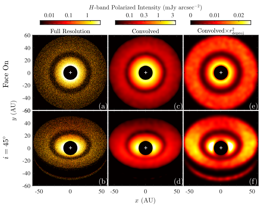
As examples, Figure 1 shows the dust surface density and scattered light images at both face on and $i=45^{\circ}$ inclination for Model 1$M_{\rm S}h$5$\alpha$1e-3. Unless otherwise noted, all images in this paper show $H$-band polarized intensity $I$, although we note that our results generally apply to total intensity images as well (see below). In panel (e) and (f), we scale the images by $r^{2}$ to compensate for the distance from the star, where $r$ is the distance from the star (deprojected in inclined cases). Unless otherwise noted, all $H$-band images and their radial profiles below have been scaled by $r^{2}$.

Fung & Chiang [32] have shown that the surface density of planet-opened gaps in 3D hydro simulations are nearly the same as gaps in 2D simulations. In this section we show that synthetic images are also practically identical between a 3D model and a model with 2D surface density manually puffed up using Equation 7.

Figure 2 shows two face-on synthetic images and their azimuthally averaged radial profile for the model 1$M_{\rm S}h$5$\alpha$1e-3. Panel (a) is from a 3D hydro simulation, while panel (b) is produced by puffing up the surface density of the model by the same assumed $h/r$ profile as in the 3D hydro calculation. Note that unlike all other images in the paper, in both panels the circumplanetary region is not excised. The gap profiles (c) from the two images are essentially identical. This result means vertical kinematic support is unimportant in the vertical distribution of material in the gap region, and we can safely puff up 2D hydro surface density structures in MCRT simulations to study gaps in scattered light.

The differences between the two images are in the local structures. First, the spiral arms are clearly more prominent in (a) than in (b), due to vertical kinematic support in planet-induced density waves [105, Dong & Fung, submitted]. Second, the circumplanetary region sticks out in (b) while it is not noticeable in (a). This is because when puffing up 2D structures into 3D, the circumplanetary region, which has a higher surface density than the surroundings, is artificially expanded in the vertical direction by the same $h/r$ as the rest of the disk. In reality though the gravity in the circumplanetary region is dominated by the planet so the actual $h/r$ of the circumplanetary region is much smaller. This leads to artificially brightening of the region in scattered light in (b). For this reason, and to avoid the artificial shadow in the outer disk produced by this structure [43, e.g.,], we excise the circumplanetary region in 2D surface density maps when puffing it up in MCRT simulations in the rest of the paper.

Figure 3 shows the radial profiles of the surface density, and both full resolution and convolved images at face-on viewing angle for three representative models with $\alpha=10^{-3}$, $h/r=0.05$, and $M_{\rm p}=2M_{\rm N}$, $1M_{\rm S}$, and $1M_{\rm J}$. The images have been scaled by $r^{2}$. Qualitatively, in all three cases, each with very different gap depths, the radial profiles of the full resolution images closely traces the variations in the surface density profiles. This general behavior has been found by Muto [61] using analytical calculations of scattered light grazing angles in disks with narrow gaps. The two deviate near the gap bottom, where the scattered light profile does not reach as deep as the surface density. Also, the outer edge of the scattered light gap lies slightly inside the surface density gap.

These observations can be qualitatively explained. Approximately, scattered light comes from a surface with optical depth of unity to the star [84]. For disks with constant $h/r$, if the surface density variation is smooth, this surface is flat at roughly a constant polar angle $\theta_{\rm surface}\propto h/r$ (i.e., not concave-up as in flared disks). In this case, at $i=0$ the $r^{2}$-scaled intensity of the scattered light at each radius is roughly proportional to the surface density of the dust above the surface, $I\propto\Sigma_{\theta>\theta_{\rm surface}}(r)$. Because $\Sigma_{\theta>\theta_{\rm surface}}(r)\propto\Sigma(r)$ for disks with constant $h/r$, it follows that $I\propto\Sigma(r)$, which is what we find. This relation breaks when the surface density fluctuation is so large that the disk surface is no longer at roughly a constant $\theta_{\rm surface}$, which happens when the gap depletion is high, and at the gap edges. Also, this analysis does not formally hold if the disk surface is flared (i.e., $h/r$ increases outward). However, gaps are local structures, and the global flareness of the disk may not significantly affect the width and depth of local structures. We will come back to this point later in Section III.6.

Convolving the full resolution image by a finite PSF smooths structures. Convolved images (dotted line) thus closely follow full resolution images outside the gap, as the variations occur on spatial scale much larger than the angular resolution ($\sim 6$AU for $\eta=0\arcsec.04$ and $d=$140 pc). Inside the gaps, convolved images have less steep edges and shallower depths.

A planet-opened gap is a perturbation on top of an initial “background” disk with no planets. The definition and characterization of a gap are relative to this background. While in simulations a planetless background can be well defined, in real observations of actual systems it is nearly impossible to do so. In addition, a complete global disk profile is often not accessible in real observations with finite inner and outer working angles. In fact, based on scattered light alone it is usually difficult to verdict whether a “gap-like” structure is indeed a planet-opened gap or not. To mimic actual observations and to maximize the applicability of the correlations derived in this work, below we will assume gaps as local structures so that its parametrization only involves its immediate neighborhood, and we will characterize an observed gap in such a way that does not require prior knowledge of the underlying planetless background disk. We emphasize this is an necessary assumption in order to construct useful empirical relations to quickly and quantitatively convert observed gap properties to planet and disk properties. For individual actual systems, whether this assumption is good or not may be indicated by the reasonableness of the fitting. More accurate assessments of the planet and disk properties require detailed modeling of individual systems with specifically designed simulations to match the 1D (or even 2D) gap profiles, instead of using parameterized gap depth and width.

The definitions of gap depth and width in surface density vary somewhat in the literature. For the former, the common practice is to define it as the ratio between the minimum $\Sigma$ inside the gap (or averaged over a finite radial range) to a fiducial “undepleted” value ($\Sigma_{0}$). What counts as $\Sigma_{0}$ varies. For the gap width, the difficulty lies in defining the two gap edges, $r_{\rm out}$ and $r_{\rm in}$ (such that $w_{\Sigma}=r_{\rm out}-r_{\rm in}$). The common practice is to define them as where $\Sigma$ reaches a certain threshold fraction of $\Sigma_{0}$ [48, e.g.,]. This class of width definitions does not work for shallow gaps in which the depletion is less than the threshold fraction. With this fixed-depth-width definition, $w_{\Sigma}$ depends on $M_{\rm p}$ and $\alpha$ in addition to $h/r$ [48, 49, e.g.,].

In this paper, we adopt dynamical definitions of the gap depth and width in both surface density and images, as illustrated in Figure 4. Our definitions work for of gaps with a wide range of depth and width. For $\Sigma$, we first find the location in the gap where $\Sigma$ reaches the minimum, $r_{\rm min,\Sigma}$. The initial value of $\Sigma$ at $r_{\rm min,\Sigma}$, $\Sigma_{0}(r_{\rm min})$, is regarded as the fiducial undepleted value. Thus $\delta_{\Sigma}$ is defined as

We then regard the inner and outer gap edges, $r_{\rm in,\Sigma}$ and $r_{\rm out,\Sigma}$, as where surface density reaches the geometric mean of the minimum and the undepleted value,

therefore the gap width $w_{\Sigma}$ is

and the normalized gap width $\Delta_{\Sigma}$ is defined as

We note $w_{\Sigma}$ has a physical unit (e.g., AU or arcsec), while $\Delta_{\Sigma}$ is dimensionless.

The definitions of gap width and gaps in scattered light are similar. We first scale the image by $r^{2}$, then find the location in the gap where $I$ reaches the minimum, $r_{\rm min,I}$ (a gap cannot be defined if the $r^{2}$-scaled intensity monotonically varies with radius). We find that in general $r_{\rm min,I}\sim r_{\rm min,\Sigma}\sim r_{\rm p}$, with small model-by-model differences. We then read the intensity at $r_{1}=2r_{\rm min,I}/3$ and $r_{2}=3r_{\rm min,I}/2$. These two locations are far away from the gap region so they are considered to be outside the influence of the gap. A fiducial “background” $I_{0}$ at $r_{\rm min}$ is subsequently defined as the geometric mean of the two points (note that this choice assumes the underlying “planetless” background profile follows a power law), $I_{0}(r_{\rm min,I})\equiv\sqrt{I(r_{1})I(r_{2})}$, and the gap depth is

The inner and outer edges of the gap, $r_{\rm in,I}$ and $r_{\rm in,I}$, are found at where $I$ reaches the geometric mean of $I_{0}$ and $I$ at $r_{\rm min,I}$.

Correspondingly, the width of the gap $w_{I}$ is defined as

and the normalized gap width $\Delta_{I}$ is

The gap parameters in surface density and in face-on images for all models are listed in Table 1.

Finally, we note that all image-related quantities, such as $\delta_{I}$, $w_{I}$, and $\Delta_{I}$, are functions of both angular resolution $\eta$, and inclination $i$, i.e., $\delta_{I}(\eta,i)$, $w_{I}(\eta,i)$, and $\Delta_{I}(\eta,i)$. We omit the variables when the context is clear.

Previous numerical studies have fit empirical relations to express $w_{\Sigma}$ and $\delta_{\Sigma}$ as functions of $[\alpha,h/r,M_{\rm p}]$. Here we derive our version based on the new definitions of depth and width in Figure 4. As discussed in Section I, analytical weakly-nonlinear theory and simple scaling relations based on torque balancing have motivated Equations 1 and 2 as possible functional forms for $w_{\Sigma}$ and $\delta_{\Sigma}$. We are able to achieve good fit for both correlations, as shown in Figure 5, by varying only the constant proportionality factor. For gap width we have

The standard deviation $\sigma$ is $9\%$ for all models. If we restrict to only the models that have been run for longer than viscous timescale ($\alpha=10^{-3}$ and $\alpha=3\times 10^{-3}$, the black points), we again recover Eqn (16) while $\sigma$ shrinks to $6\%$. We note that if we adopt the Kanagawa et al. [48] definition of the gap width, we do recover their $\Delta_{\Sigma}=0.41q^{1/2}(h/r)^{-3/4}\alpha^{-1/4}$ correlation (with a standard deviation of 17%). However we prefer our dynamical definition of the gap width over defining the width as the distance between two points on the edges with a fixed depletion factor for a few reasons. First, the latter does not work for shallow gaps opened by relatively low mass planets, and in real observations such gaps are more common than deeper gaps opened by more massive planets, due to the higher occurrence rate of smaller planets than their more massive siblings [13]. Second, adopting the latter definition returns a less robust correlation between the gap width in images and the gap width in surface density (not shown). Third, while the Kanagawa et al. [48] correlation is a pure empirical correlation synthesized from simulations within a confined parameter space, our Eqn (16) has some theoretical footing from gap opening theory, thus more robust when applying to real systems that may lie outside the parameter space explored by our models.

For gap depth, we have

with $\sigma=17\%$ for all but the three $M_{\rm p}=M_{\rm J}$ and $h/r=0.05$ models, which have the largest thermal masses in our models, $M_{\rm p}=8M_{\rm thermal}$, and so their gap opening process is in the strongly nonlinear regime and the analytical torque balancing calculations break. We have experimented with freeing the power law indexes in the fit; overall no significant improvement is found.

We thus conclude that the gap width and depth definitions in Figure 4 successfully capture the physics of gap opening as argued by analytical theories. One thing to note is that $h/r$ can now be directly constrained based on measured gap properties. Assuming hydrostatic equilibrium in the vertical direction, scale height $h/r$ is related to disk temperature $T$ at each radius as

where $v_{\rm k}$ is the Keplerian speed, and $\mu$ is the mean molecular weight. Thus, our constraints on $h/r$ based on measured gap properties can be used to infer the midplane temperature of the disk at the location of the gap.

At $i=0$, we measure 4 quantities for each model for a given $\eta$: $\Delta_{\Sigma}$, $\delta_{\Sigma}$, $\Delta_{I}(\eta)$, and $\delta_{I}(\eta)$. Figure 6 compares $\Delta_{\Sigma}$ with $\Delta_{I}(\eta)$, and $\delta_{\Sigma}$ with $\delta_{I}(\eta)$, for both $\eta=0$ and $\eta=0\arcsec.04$.

In full resolution images, it is well approximated that $\Delta_{I}(0)=\Delta_{\Sigma}$, with a standard deviation of 7% for all gaps. For the depth, $\delta_{I}(0)$ is close to $\delta_{\Sigma}$ for shallow gaps ($\delta_{\Sigma}\lesssim 5$), but deviates from $\delta_{\Sigma}$ for deeper gaps. Once convolved, we expect the gap to become shallower and narrower, and we expect the effect of PSF smearing to depend on the ratio of

since with higher angular resolution (smaller $\eta$) and/or wider gaps (bigger $w_{I}$), the intrinsic gap profile at $\eta=0$ is better preserved; and vice versa. This is confirmed in the figure — for wider gaps $\Delta_{I}(\eta)$ well correlates with $\Delta_{\Sigma}$ (as well as $\Delta_{I}(0)$), while narrower gaps becomes noticeably wider with finite $\eta$. For the depth, PSF smearing makes the gap shallower in all cases.

Quantitatively, we find $\Delta_{I}(\eta)$ is correlated to $\Delta_{\Sigma}(\eta)$, $\beta$, and $\delta_{I}$ in the following way,

with $\sigma=9$%. In the high angular resolution limit ($\beta\rightarrow 0$), $\Delta_{I}\rightarrow\Delta_{\Sigma}$. For the gap depth, we find

with $\sigma=20$%. In the high angular resolution ($\beta\rightarrow 0$) and shallow gap limit ($\delta_{\Sigma}\rightarrow 1$), $\delta_{I}\rightarrow\delta_{\Sigma}$. Both equations are invertible and it is straight forward to obtain $\delta_{\Sigma}$ and $w_{\Sigma}$, given $\delta_{I}$, $w_{I}$, and $\eta$. These correlations are synthesized for the parameter space of $0.2\lesssim\Delta_{I}\lesssim 0.5$ and $1\lesssim\delta_{I}\lesssim 50$; we caution their applications to the parameter space beyond.

In this section, we compare the radial profile of face-on images to the radial profile along the major axis of disks at modest inclinations ($i\lesssim 45^{\circ}$). In the latter, the radial profiles are averaged over a wedge of $\pm 10^{\circ}$ from the major axis centered on the central star, as indicated in Figure 8(c). We note that in inclined disks, equal distance points from the center approximately fall on ellipses not centered on the star (shifted along the minor axis), because these ellipses are at non-zero height [81, Fig. 1 in]. Therefore, strictly speaking the major axis going through the star is not the major axis of the gap ellipse (the two are parallel to each other). Nevertheless, measuring the radial profile along the major axis centered on the star is common practice in the field [34, 15, e.g.,]; to facilitate the applications of our results, we do the same. The scattering angle along the major axis is close to $90^{\circ}$, the same as in face-on images. Therefore, the relative radial profile along the major axis is minimally affected by dust scattering properties.

Major axis radial profiles at modest inclinations closely follow their face-on counterparts. Figure 8 compares the two for three representative models with $\alpha=10^{-3}$, $h/r=0.05$, and $M_{\rm p}=2M_{\rm N}$, $1M_{\rm S}$, and $1M_{\rm J}$. In all cases the gap region in the inclined disk is slightly shifted inward comparing with the face-on disk, due to the the inclination effect discussed above. The outer gap edge is shifted slightly more than the inner edge. Figure 9 shows the gap profile at $i=0$, $15^{\circ}$, $30^{\circ}$, and $45^{\circ}$ for both the full resolution and convolved images of model 1$M_{\rm S}h$5$\alpha$1e-3. Intuitively, the differences between inclined and face-on images increase with $i$. When $i$ approaches 0, the differences diminish.

Quantitatively, the gap width in inclined disks agree with face-on disks very well,

with a standard deviation of 5% between the two. On the other hand, inclined images have systematically shallower gaps,

with a standard deviation of 9% ($i$ is in the unit of degree). The effect of inclination on $\delta_{I}(i)$ is weak — with $i=45^{\circ}$, the gap depth is only reduced by 10%. Figure 10 compares $\Delta_{I}(45^{\circ})$ vs $\Delta_{I}(0)$, and $\delta_{I}(45^{\circ})$ vs $\delta_{I}(0)$ for 6 representative models.

So far, $h/r$ is taken to be a constant in our models (i.e., no radial dependence). This choice results in a flat disk surface, which simplifies the problem in our qualitative analysis of the physical picture, and enables us to obtain a straightforward intuition to why scattered light features closely follow the structures in surface density (Section III.1). However, real disks passively heated by the central star may be flared, with $h/r\propto r^{\gamma}$ and $\gamma>0$ [12, e.g.,]. For example, by modeling the spectral energy distribution (SED) and resolved mm observations, Andrews et al. [4] obtained $\gamma=0.19\pm 0.1$ for a sample of 12 transitional disks. This surface flareness certainly affects the scattered light distribution in disks; for example, flared disks have surface brightness decreasing slower with radius than flat disks. This may affect the width and depth of gaps in images, and alter the surface density profiles slightly (through Eqns 17 and 16).

However, the narrow gaps explored in this study are essentially local structures. In this case, the $h/r$ variation across the gap under a reasonable $\gamma$ (e.g., $\gamma\lesssim 0.25$) may be too small to produce any significant effect. To test this hypothesis, we carry out experiments and compare three models with different $\gamma$’s, but otherwise the same parameters, to examine the dependence of gap width and depth on $\gamma$. The results are shown in Figure 11. With $h/r=0.05$ at $r_{\rm p}=30$ AU, $\alpha=10^{-3}$, and $M_{\rm p}=1M_{\rm S}$, the three models with $\gamma=0$ (flat disk), 0.1, and 0.25 (flare disks) produce very similar gap properties in both the surface density and scattered light (the global scattered light profile in these models are of course different — flared disks have a brighter outer disk — as expected). Specifically, for $\Delta_{\Sigma}$ and $\Delta_{I}$, all three models return essentially the same values; for $\delta_{\Sigma}$, the two flared models have measurements higher than the flat model by $\sim 5\%$; and for $\delta_{I}(\eta|0)$, the two flared models differ from the flat model by about 10%. Therefore, we tentatively conclude that under reasonable flareness ($\gamma\lesssim 0.25$), the flaring of the disk does not significantly affect the gap properties in both the density and image space for narrow gaps as in this example; subsequently, we expect the correlations derived in this paper to hold to a good approximation. A full parameter space exploration is needed to firmly establish this statement for more general cases.

Fitted correlations 16–23 compose a complete set of equations to link $[\Delta_{I},\delta_{I}]$ with $[M_{\rm p},h/r,\alpha]$. Once a narrow gap ($\Delta_{I}(\eta,i)\lesssim 0.5$) is identified in scattered light of a disk at a modest inclination ($i\lesssim 45^{\circ}$) with both the inner and outer gap edges clearly revealed, one can follow the following steps to link observed gap properties to planet and disk parameters $[M_{\rm p},h/r,\alpha]$:

1. I

   Use Equations 22–23 to eliminate the effect of inclination: $\delta_{I}(\eta,i)\rightarrow\delta_{I}(\eta,0)$, $\Delta_{I}(\eta,i)\rightarrow\Delta_{I}(\eta,0)$;

2. II

   Use Equations 19–21 to eliminate the effect of finite angular resolution, and link images to surface density: $\delta_{I}(\eta,0)\rightarrow\delta_{\Sigma}$, $\Delta_{I}(\eta,0)\rightarrow\Delta_{\Sigma}$;

3. III

   Finally, Equations 16 and 17 link the gap properties in surface density to $[M_{\rm p},h/r,\alpha]$. Note that normally $h/r$ can be constrained directly from the gap width, and it leaves the quantity $q^{2}/\alpha$ to be constrained from the gap depth.

We note that these correlations are derived for polarized intensity at $H$-band, but they also apply to total intensity images, and/or images in other spectral bands within a factor of $\sim 2$ difference in wavelength from $H$-band (as long as the signals are dust scattering dominated), because both depth and width are measured in a relative sense, and face-on radial profiles and major axis radial profiles in inclined images minimize the dependence on scattering angles. Finally, we emphasize that a key precondition when applying these correlations to actual systems is that the gap bottom needs to be detected (i.e., the gap bottom in images should be above the detection threshold). If not, the gap depth becomes illy defined.

In simulating the gap images and deriving the correlations, we have made a number of assumptions in disk structures and modeling. Here we comment on the effects of these assumptions, and caution the readers about the caveats when applying our results to real disks.

1. 1.

   Jang-Condell & Turner [44, Figure 2] highlighted that the outer gap edge may receive extra stellar radiation due to the depletion of material inside the gap, leading to higher temperature thus higher $h/r$ (see also Jang-Condell 42, Isella & Turner 41). However, whether this effect can increase the contrast of the gap at the outer edge need additional investigations. Fung & Chiang [32, Figure 6] showed that gas inside the gap and around the gap edges circulate, therefore the heating at the outer edge is redistributed to a much larger region in the disk, weakening this thermal feedback. Future coupled hydro-radiation-transfer simulations are needed to quantify this effect.

2. 2.

   Ribas et al. [75, see also ] showed that the fraction of stars with protoplanetary disks, indicated by their infrared excesses, drops on a time scale of about 3 Myr. The timescale that a planet takes to fully open a gap with a gap width of $6h$ (i.e., our gap width) is approximately the viscous timescale to cross $6h$, $\tau_{\nu}=6/(\alpha(h/r)\Omega_{\rm K})$. With $\alpha(h/r)/(r_{\rm p}/30\rm{AU})^{1.5}\lesssim 10^{-4}$, $\tau_{\nu}$ is longer than 3Myr. Therefore, in low viscosity disks, very young systems, and large separations from the center, gaps may not reach their final depth and width, which invalids the $[M_{\rm p},h/r,\alpha]-[\Delta_{\Sigma},\delta_{\Sigma}]$ correlations synthesized in this work and in others. This gap opening timescale issue is however irrelevant to the $[\delta_{I},\Delta_{I}]-[\delta_{\Sigma},w_{\Sigma}]$ conversions, and we expect them to hold even when the gap is only partially opened.

3. 3.

   In our MCRT simulations, no noise is added into the images (apart from the intrinsic Poisson noise due to finite number of photons), thus the gap bottom reach their theoretically minimum. If in real observations the gap bottom reaches the noise level, the measured gap depth, and the derived planet mass, will be their lower limits, while the measured gap width, and the derived disk scale height, will be their upper limits.

HD 97048 is a $\sim 2.5M_{\odot}$ Herbig Ae/Be star located at $\sim$158 pc [93, 96] surrounded by a protoplanetary disk several hundreds of AU in size. The disk is inclined at $\sim 40^{\circ}$ based on mm observations [99, 95]. Maaskant et al. [57] first suggested that this disk may be gap/cavity harboring based on SED modeling. Very recently, VLT/SPHERE $J$-band imaging in both polarized and total intensity found multiple rings and gaps in this system [34]. In addition, the mm dust continuum counterparts of some of these structures may have been found by van der Plas et al. [95], suggesting the scattered light gaps and rings are likely to be physical density structures instead of shadow effects.

Here we focus on the “gap 2” in the $J$-band VLT/SPHERE dataset [34]. Comparing with the other gaps, gap 2 is well detected in both polarized and total intensity, with inner and outer edges clearly resolved. We obtain $h/r=0.06$ at the location of the gap ($0\arcsec.67$; 106 AU), and constrain the planet mass to be between 0.4–4 $M_{\rm J}$ for $10^{-4}\lesssim\alpha\lesssim 10^{-2}$. By analyzing the offset of the center of the gap ellipse from the star, Ginski et al. [34] determined that at the gap location the disk’s surface is at $\theta\sim 0.2$ rad. Therefore, the disk surface is at about 3–4 scale heights away from the disk midplane, which is reasonable [12, e.g.,] (we note that in our MCRT simulations the disk surface is also generally about 4 scale heights away from the midplane). Ginski et al. [34] ruled out the presence of planets more massive than $2M_{\rm J}$ at the gap location (assuming the BT-SETTL isochrones; Allard et al. 2). Comparing with our constraints on the planet mass, this suggests the viscosity in the gap may be low, $\alpha\lesssim 10^{-3}$.

TW Hya is a $\sim 0.8M_{\odot}$ K6 star located at 54 pc [90, 91]. The nearly face-on disk ($i\sim 7^{\circ}$; Qi et al. 69) has been imaged by HST [17, 16], Gemini/GPI [73], Subaru/HiCIAO [1], and VLT/SPHERE [92], and multiple gaps have been identified in scattered light: one at $\sim$80 AU, one at $\sim 20$ AU, and one at $\lesssim 6$ AU. The mm continuum counterpart of the 20 AU gap may have been identified by Andrews et al. [5] in ALMA observations at a slightly larger radius (possibly caused by the dust filtration effect).

Here we examine two gaps in the system: the one at $\sim 20$, and the one at $\sim 80$ AU, in the $H$-band VLT/SPHERE dataset van Boekel et al. [92, Fig. 3]. Due to the low inclination, the azimuthally averaged radial profile is used. For the inner gap, $h/r$ at the gap location ($0\arcsec.37$; 20 AU) is 0.068, and the planet mass is between 0.05–0.5 $M_{\rm J}$ for $10^{-4}\lesssim\alpha\lesssim 10^{-2}$; for the outer gap, $h/r$ at the gap location ($1\arcsec.5$; 81 AU) is 0.055, and the planet mass is between 0.03–0.3 $M_{\rm J}$ for $10^{-4}\lesssim\alpha\lesssim 10^{-2}$.

Using hydro+MCRT simulations, Rapson et al. [73] tentatively fit the observed gap profile at $\sim 20$ AU in the Gemini/GPI dataset using a $0.16M_{\rm J}$ planet at 21 AU assuming $\alpha=10^{-3}$ and $h/r=0.068$. Their results agree well with our findings. van Boekel et al. [92] used radiative transfer simulations to transform the scattered light map into surface density and scale height profiles. At 20 AU they obtained $h/r=0.05$, while at $80$ AU they obtained $h/r=0.08$. Subsequently, assuming $\alpha=2\times 10^{-4}$, they derived the masses of the planets at 20 and 80 AU to be 0.05$M_{\rm J}$ and 0.11$M_{\rm J}$, based on the a similar version of Eqn 17 in Duffell [25]. While their $h/r$ and $M_{\rm p}$ at the inner gap is broadly consistent with our results, our estimated $h/r$ for the outer gap is significantly lower (and also lower than our estimated $h/r$ at 20 AU), resulting in a lower estimate for $M_{\rm p}$ as well. This may indicate that the 80 AU gap is not opened by a planet; alternatively, this may be because our assumption of the gap structure being local is no longer valid for the 80 AU gap, which may lie in the shadow created by the inner disk thus the underlying “background” is no longer smooth.

HD 169142 is a $\sim 2M_{\odot}$ Herbig Ae star located at 145 pc [71, 83]. It has a prominent protoplanetary disk at an inclination of $13^{\circ}$, determined from gas kinematics [71, 64]. A narrow gap around 50 AU was first discovered in $H$-band VLT/NACO polarized light imaging [70], and subsequently found by Subaru/HiCIAO [59] and in dust thermal emission at 7mm by VLA [63]. The radius-varying disk profile was interpreted as two power laws in the inner and outer disks joined by a transition region in between by Momose et al. [59]. Osorio et al. [63] also discovered a blob in the 7mm VLA dataset residing right inside the gap, with an estimated total mass of $6\times 10^{-6}M_{\odot}$ in dust. Through radiative transfer modeling, Wagner et al. [97] determined that this gap cannot be explained by shadow effects caused by the inner disk, leaving the planet-sculpting scenario as a favorite hypothesis. By comparing the apparent gap depth in 7mm observations with their $M_{\rm p}-\delta_{\Sigma}$ relation, Kanagawa et al. [47] estimated the mass of the putative planet to be $M_{\rm p}\gtrsim 0.4M_{\rm J}$. As Rosotti et al. [76] pointed out, such estimate is risky as mm observations trace mm-sized grains, which can have substantially different spatial distribution from the gas due to dust/gas coupling effects. The disk has another inner gap at $\sim 25$ AU [40, 70], and a companion candidate at the edge of the inner gap [74, see also Biller et al. 8].

Here we examine the gap at 40–70 AU in the Subaru/HiCIAO $H$-band dataset [59]. Due to the low inclination, we adopt azimuthally averaged radial profile after deprojecting the disk Momose et al. [59, Fig. 2; assuming = i 13 ∘ and position angle = 5∘]. We derive $h/r$ at the gap location ($0\arcsec.35$; 51 AU) to be 0.08, and the planet mass is between 0.2–2.1 $M_{\rm J}$ for $10^{-4}\lesssim\alpha\lesssim 10^{-2}$.

LkCa 15 is a $\sim 1M_{\odot}$ K3 star located at 140 pc [66, 80]. Using Spitzer IRS spectrum modeling, Espaillat et al. [28] identified the system as a transitional disk with an outer disk, an inner disk, and a gap in between. SMA mm observations resolved the gap and determined its outer radius to be 50 AU in dust continuum emission [4]. The gap has since been resolved in scattered light by Subaru/HiCIAO [86], Gemini/NICI [87], and VLT/SPHERE [88, 89] in both total and polarized intensity. The latest VLT/SPHERE observations by Thalmann et al. [89] at multiple optical to NIR bands clearly showed that the system has an substantial inner disk, and the gap is narrow enough ($\Delta_{I}<0.5$) to warrant the hypothesis that it may be opened by a single planet. The inclination of the disk is $\sim 50^{\circ}$ based on mm observations [4, 66, 94].

Here we examine the gap profile along the major axis of the disk in the VLT/SPHERE $H$-band polarized intensity dataset presented in Thalmann et al. [89]. We derive $h/r$ at the gap location ($0\arcsec.26$; 36 AU) to be 0.07, and the planet mass is between 0.15–1.5 $M_{\rm J}$ for $10^{-4}\lesssim\alpha\lesssim 10^{-2}$.

LkCa has several detected planet candidates. Using non-redundant aperture masking interferometry on Keck, Kraus & Ireland [53] identified a point source at a deprojected distance of $\sim 20$ AU from the star. Recently, Sallum et al. [78] reported the detections of two additional point sources in the system with LBT/LBTI and Magellan/MagAO. The three planet candidates in Sallum et al. [78] are located between 15–19 AU. We note that these planet candidates are unlikely to be the one responsible for maintaining the gap edge in scattered light at $\sim 50$ AU (i.e., the one whose properties we are inferring here), as they are too far away from the gap edge. The radial profile of the gap (Figure 12d) is not inconsistent with the gap being opened by just one planet. Additional planets at $r\lesssim 20$ AU with sufficiently low mass will not significantly affect the gap opened by the outer planet.

RX J1615.3-3255 (hereafter J1615) is a $1.1M_{\odot}$ K5 star at 185 pc [102, 98, 4]. The system has a gap with an outer radius of $\sim 20-30$ AU, revealed in mm dust continuum emission first by SMA [4] and subsequently by ALMA [94]. The disk has a modest inclination, $i\sim 45^{\circ}$. Recently, de Boer et al. [15] resolved this system in scattered light at multiple optical-to-NIR wavelengths using VLT/SPHERE, and identified multiple gaps and rings in the system.

Here we examine the the major axis profile of the gap at $\sim 90$ AU in the $J$-band VLT/SPHERE dataset presented by de Boer et al. [15, marked “G” in Fig. 1]. We derive $h/r$ at the gap location ($0\arcsec.52$; 96 AU) to be 0.06, and the planet mass is between 0.07–0.7 $M_{\rm J}$ for $10^{-4}\lesssim\alpha\lesssim 10^{-2}$.

By analyzing the alternating bright/dark pattern on the rings, de Boer et al. [15] found tentative evidence to suggest that the rings in J1615 might be caused by shadows (i.e., variation in scale height instead of surface density). At the moment the evidence is inclusive.

References

- [1] Akiyama, E., Muto, T., Kusakabe, N., et al. 2015, ApJ, 802, L17
- [2] Allard, F., Homeier, D., & Freytag, B. 2011, in Astronomical Society of the Pacific Conference Series, Vol. 448, 16th Cambridge Workshop on Cool Stars, Stellar Systems, and the Sun, ed. C. Johns-Krull, M. K. Browning, & A. A. West, 91
- [3] ALMA Partnership, Brogan, C. L., Pérez, L. M., et al. 2015, ApJ, 808, L3
- [4] Andrews, S. M., Wilner, D. J., Espaillat, C., et al. 2011, ApJ, 732, 42
- [5] Andrews, S. M., Wilner, D. J., Zhu, Z., et al. 2016, ApJ, 820, L40
- [6] Baraffe, I., Chabrier, G., Allard, F., & Hauschildt, P. H. 1998, A&A, 337, 403
- [7] Beuzit, J.-L., Feldt, M., Dohlen, K., et al. 2008, in Society of Photo-Optical Instrumentation Engineers (SPIE) Conference Series, Vol. 7014, Society of Photo-Optical Instrumentation Engineers (SPIE) Conference Series
- [8] Biller, B. A., Males, J., Rodigas, T., et al. 2014, ApJ, 792, L22
- [9] Bowler, B. P. 2016, ArXiv e-prints, arXiv:1605.02731
- [10] Brandt, T. D., McElwain, M. W., Turner, E. L., et al. 2014, ApJ, 794, 159
- [11] Carrasco-González, C., Henning, T., Chandler, C. J., et al. 2016, ApJ, 821, L16
- [12] Chiang, E. I., & Goldreich, P. 1997, ApJ, 490, 368
- [13] Cumming, A., Butler, R. P., Marcy, G. W., et al. 2008, PASP, 120, 531
- [14] D’Angelo, G., Lubow, S. H., & Bate, M. R. 2006, ApJ, 652, 1698
- [15] de Boer, J., Salter, G., Benisty, M., et al. 2016, ArXiv e-prints, arXiv:1610.04038
- [16] Debes, J. H., Jang-Condell, H., & Schneider, G. 2016, ApJ, 819, L1
- [17] Debes, J. H., Jang-Condell, H., Weinberger, A. J., Roberge, A., & Schneider, G. 2013, ApJ, 771, 45
- [18] Dodson-Robinson, S. E., & Salyk, C. 2011, ApJ, 738, 131
- [19] Dong, R., & Dawson, R. 2016, ApJ, 825, 77
- [20] Dong, R., Fung, J., & Chiang, E. 2016, ApJ, 826, 75
- [21] Dong, R., Rafikov, R. R., & Stone, J. M. 2011a, ApJ, 741, 57
- [22] Dong, R., Rafikov, R. R., Stone, J. M., & Petrovich, C. 2011b, ApJ, 741, 56
- [23] Dong, R., Zhu, Z., & Whitney, B. 2015, ApJ, 809, 93
- [24] Dong, R., Rafikov, R., Zhu, Z., et al. 2012, ApJ, 750, 161
- [25] Duffell, P. C. 2015, ApJ, 807, L11
- [26] Duffell, P. C., & Dong, R. 2015, ApJ, 802, 42
- [27] Duffell, P. C., & MacFadyen, A. I. 2013, ApJ, 769, 41
- [28] Espaillat, C., D’Alessio, P., Hernández, J., et al. 2010, ApJ, 717, 441
- [29] Follette, K. B., Grady, C. A., Swearingen, J. R., et al. 2015, ApJ, 798, 132
- [30] Fouchet, L., Gonzalez, J.-F., & Maddison, S. T. 2010, A&A, 518, A16
- [31] Fung, J. 2015, PhD thesis, University of Toronto, Canada
- [32] Fung, J., & Chiang, E. 2016, ArXiv e-prints, arXiv:1606.02299
- [33] Fung, J., Shi, J.-M., & Chiang, E. 2014, ApJ, 782, 88
- [34] Ginski, C., Stolker, T., Pinilla, P., et al. 2016, ArXiv e-prints, arXiv:1609.04027
- [35] Gonzalez, J.-F., Pinte, C., Maddison, S. T., Ménard, F., & Fouchet, L. 2012, A&A, 547, A58
- [36] Goodman, J., & Rafikov, R. R. 2001, ApJ, 552, 793
- [37] Hashimoto, J., Tamura, M., Muto, T., et al. 2011, ApJ, 729, L17
- [38] Hashimoto, J., Dong, R., Kudo, T., et al. 2012, ApJ, 758, L19
- [39] Hernández, J., Hartmann, L., Calvet, N., et al. 2008, ApJ, 686, 1195
- [40] Honda, M., Maaskant, K., Okamoto, Y. K., et al. 2012, ApJ, 752, 143
- [41] Isella, A., & Turner, N. 2016, ArXiv e-prints, arXiv:1608.05123
- [42] Jang-Condell, H. 2008, ApJ, 679, 797
- [43] —. 2009, ApJ, 700, 820
- [44] Jang-Condell, H., & Turner, N. J. 2012, ApJ, 749, 153
- [45] —. 2013, ApJ, 772, 34
- [46] Jin, S., Li, S., Isella, A., Li, H., & Ji, J. 2016, ApJ, 818, 76
- [47] Kanagawa, K. D., Muto, T., Tanaka, H., et al. 2015, ApJ, 806, L15
- [48] —. 2016a, PASJ, 68, 43
- [49] Kanagawa, K. D., Tanaka, H., Muto, T., & Tanigawa, T. 2016b, ArXiv e-prints, arXiv:1609.02706
- [50] Kim, S.-H., Martin, P. G., & Hendry, P. D. 1994, ApJ, 422, 164
- [51] Kley, W., & Dirksen, G. 2006, A&A, 447, 369
- [52] Konishi, M., Grady, C. A., Schneider, G., et al. 2016, ArXiv e-prints, arXiv:1601.06560
- [53] Kraus, A. L., & Ireland, M. J. 2012, ApJ, 745, 5
- [54] Lenzen, R., Hartung, M., Brandner, W., et al. 2003, in Proc. SPIE, Vol. 4841, Instrument Design and Performance for Optical/Infrared Ground-based Telescopes, ed. M. Iye & A. F. M. Moorwood, 944–952
- [55] Li, H., Finn, J. M., Lovelace, R. V. E., & Colgate, S. A. 2000, ApJ, 533, 1023
- [56] Lin, M.-K., & Papaloizou, J. C. B. 2010, MNRAS, 405, 1473
- [57] Maaskant, K. M., Honda, M., Waters, L. B. F. M., et al. 2013, A&A, 555, A64
- [58] Macintosh, B. A., Graham, J. R., Palmer, D. W., et al. 2008, in Society of Photo-Optical Instrumentation Engineers (SPIE) Conference Series, Vol. 7015, Society of Photo-Optical Instrumentation Engineers (SPIE) Conference Series
- [59] Momose, M., Morita, A., Fukagawa, M., et al. 2015, ArXiv e-prints, arXiv:1505.04937
- [60] Mouillet, D., Lagrange, A. M., Augereau, J. C., & Ménard, F. 2001, A&A, 372, L61
- [61] Muto, T. 2011, ApJ, 739, 10
- [62] Muto, T., Suzuki, T. K., & Inutsuka, S.-i. 2010, ApJ, 724, 448
- [63] Osorio, M., Anglada, G., Carrasco-González, C., et al. 2014, ApJ, 791, L36
- [64] Panić, O., Hogerheijde, M. R., Wilner, D., & Qi, C. 2008, A&A, 491, 219
- [65] Perrot, C., Boccaletti, A., Pantin, E., et al. 2016, A&A, 590, L7
- [66] Piétu, V., Dutrey, A., & Guilloteau, S. 2007, A&A, 467, 163
- [67] Pinilla, P., Birnstiel, T., & Walsh, C. 2015a, A&A, 580, A105
- [68] Pinilla, P., de Juan Ovelar, M., Ataiee, S., et al. 2015b, A&A, 573, A9
- [69] Qi, C., Ho, P. T. P., Wilner, D. J., et al. 2004, ApJ, 616, L11
- [70] Quanz, S. P., Avenhaus, H., Buenzli, E., et al. 2013, ApJ, 766, L2
- [71] Raman, A., Lisanti, M., Wilner, D. J., Qi, C., & Hogerheijde, M. 2006, AJ, 131, 2290
- [72] Rapson, V. A., Kastner, J. H., Andrews, S. M., et al. 2015a, ApJ, 803, L10
- [73] Rapson, V. A., Kastner, J. H., Millar-Blanchaer, M. A., & Dong, R. 2015b, ApJ, 815, L26
- [74] Reggiani, M., Quanz, S. P., Meyer, M. R., et al. 2014, ApJ, 792, L23
- [75] Ribas, Á., Merín, B., Bouy, H., & Maud, L. T. 2014, A&A, 561, A54
- [76] Rosotti, G. P., Juhasz, A., Booth, R. A., & Clarke, C. J. 2016, MNRAS, 459, 2790
- [77] Ruge, J. P., Wolf, S., Uribe, A. L., & Klahr, H. H. 2013, A&A, 549, A97
- [78] Sallum, S., Follette, K. B., Eisner, J. A., et al. 2015, Nature, 527, 342
- [79] Shakura, N. I., & Sunyaev, R. A. 1973, A&A, 24, 337
- [80] Simon, M., Dutrey, A., & Guilloteau, S. 2000, ApJ, 545, 1034
- [81] Stolker, T., Dominik, C., Min, M., et al. 2016a, ArXiv e-prints, arXiv:1609.09505
- [82] Stolker, T., Dominik, C., Avenhaus, H., et al. 2016b, ArXiv e-prints, arXiv:1603.00481
- [83] Sylvester, R. J., Skinner, C. J., Barlow, M. J., & Mannings, V. 1996, MNRAS, 279, 915
- [84] Takami, M., Hasegawa, Y., Muto, T., et al. 2014, ApJ, 795, 71
- [85] Tamura, M., Hodapp, K., Takami, H., et al. 2006, in Proc. SPIE, Vol. 6269, Society of Photo-Optical Instrumentation Engineers (SPIE) Conference Series, 62690V
- [86] Thalmann, C., Grady, C. A., Goto, M., et al. 2010, ApJ, 718, L87
- [87] Thalmann, C., Mulders, G. D., Hodapp, K., et al. 2014, A&A, 566, A51
- [88] Thalmann, C., Mulders, G. D., Janson, M., et al. 2015, ApJ, 808, L41
- [89] Thalmann, C., Janson, M., Garufi, A., et al. 2016, ApJ, 828, L17
- [90] Torres, C. A. O., Quast, G. R., da Silva, L., et al. 2006, A&A, 460, 695
- [91] Torres, C. A. O., Quast, G. R., Melo, C. H. F., & Sterzik, M. F. 2008, Young Nearby Loose Associations, ed. B. Reipurth, 757
- [92] van Boekel, R., Henning, T., Menu, J., et al. 2016, ArXiv e-prints, arXiv:1610.08939
- [93] van den Ancker, M. E., de Winter, D., & Tjin A Djie, H. R. E. 1998, A&A, 330, 145
- [94] van der Marel, N., van Dishoeck, E. F., Bruderer, S., Pérez, L., & Isella, A. 2015, A&A, 579, A106
- [95] van der Plas, G., Wright, C. M., Ménard, F., et al. 2016, ArXiv e-prints, arXiv:1609.02488
- [96] van Leeuwen, F. 2007, A&A, 474, 653
- [97] Wagner, K. R., Sitko, M. L., Grady, C. A., et al. 2015, ApJ, 798, 94
- [98] Wahhaj, Z., Cieza, L., Koerner, D. W., et al. 2010, ApJ, 724, 835
- [99] Walsh, C., Juhász, A., Meeus, G., et al. 2016, ArXiv e-prints, arXiv:1609.02011
- [100] Weinberger, A. J., Becklin, E. E., Schneider, G., et al. 1999, ApJ, 525, L53
- [101] Whitney, B. A., Robitaille, T. P., Bjorkman, J. E., et al. 2013, ApJS, 207, 30
- [102] Wichmann, R., Krautter, J., Covino, E., et al. 1997, A&A, 320, 185
- [103] Wolf, S., & D’Angelo, G. 2005, ApJ, 619, 1114
- [104] Yen, H.-W., Liu, H. B., Gu, P.-G., et al. 2016, ApJ, 820, L25
- [105] Zhu, Z., Dong, R., Stone, J. M., & Rafikov, R. R. 2015, ApJ, 813, 88
- [106] Zhu, Z., Nelson, R. P., Dong, R., Espaillat, C., & Hartmann, L. 2012, ApJ, 755, 6
- [107] Zhu, Z., Nelson, R. P., Hartmann, L., Espaillat, C., & Calvet, N. 2011, ApJ, 729, 47
- [108] Zhu, Z., Stone, J. M., & Rafikov, R. R. 2013, ApJ, 768, 143
- [109] Zhu, Z., Stone, J. M., Rafikov, R. R., & Bai, X.-n. 2014, ApJ, 785, 122