A square entropy stable flux limiter
for $P_{N}P_{M}$ schemes

Two of the most popular families of high order schemes for hyperbolic conservation laws are either reconstruction-based finite volume schemes, or discontinuous Galerkin (DG) methods that directly evolve the expansion coefficients of a piecewise polynomial data representation, and thus in principle do not need any reconstruction stage. The $P_{N}P_{M}$ philosophy introduced in [8, 7] provides a unified framework for the treatment of both approaches. At this point it is important to stress that reconstruction operators have already been used in connection with the DG method before, but only in the context of accuracy-enhancing postprocessors, which are applied to the discrete solution only once at the end of the simulation, see [24, 5], or as nonlinear moment limiters, in order to control spurious oscillations at shock waves, see [22, 23, 2]. Instead, the use of a reconstruction operator as a mechanism to enhance the accuracy of the DG scheme within each time step has been proposed for the first time within the $P_{N}P_{M}$ framework [8, 7]. Similar reconstruction-based DG schemes have subsequently been developed and applied also for example in [19, 20, 29].

In the context of finite volume schemes, high order of accuracy in space is achieved by reconstructing a high order piecewise polynomial representation of the solution (say, an ENO or WENO polynomial) from the known cell averages [16, 18, 3, 26]. An example for a high order fully discrete one-step method following this approach is the ADER scheme that is based on the approximate solution of generalized Riemann problems arising from the piecewise polynomial reconstruction of the data, see e.g. [25, 27, 28, 1, 4, 14] for more details. Methods that only evolve cell averages in time have the advantage that they can use large time-steps (CFL $<$ 1), but this comes at the cost of requiring large reconstruction stencils.

In DG schemes, on the other hand, the high order spatial accuracy derives from the fact that the discrete solution of the PDE is directly represented and evolved terms of piecewise polynomials of degree $N$ in space. At very high order, however, this requires very small time steps (CFL $<1/(2N+1)$). A natural approach for reaching higher accuracy in the DG framework is then to also include a suitable reconstruction procedure in the scheme. Since more degrees of freedom are available in each cell, we can work with compact reconstruction stencils and still keep a larger CFL number, see [8]. This is the basic idea of the $P_{N}P_{M}$ method: The solution is represented in a finite element space of piecewise polynomials of degree $N\geq 0$ (hence the $P_{N}$ in the name of the method) and at each time step before the time evolution is carried out, a high order reconstruction of piecewise polynomials of degree $M\geq N$ is computed (hence the $P_{M}$). In this framework, the pure DG method can be viewed as a $P_{N}P_{N}$ scheme, while the case $P_{0}P_{M}$ corresponds to the high order finite volume schemes. For $N>0$ and $M>N$ a family of hybrid schemes emerges.

The $P_{N}P_{M}$ method has already been successfully applied to a variety of complex flow problems, including viscous terms, non-conservative products and stiff source terms, see [8, 7, 9, 11], but our understanding of its analytical properties has not reached a mature level yet. In particular, it was observed that even in the $1D$ case for scalar, linear problems, the method is in general not strictly $L^{2}$-diminishing [12, 6] and the famous cell square entropy inequality of Jiang and Shu [17] for DG schemes is not valid for $M>N$.

In this paper, we extend the technique of Jiang and Shu to the case $M>N$ and derive a modified sufficient criterion for entropy stability that reduces to the original criterion of Jiang and Shu for $M=N$. We demonstrate why this criterion is in general not satisfied for problems with large jumps in the solution. In the linear case the new condition is a simple algebraic relation between the jump in the reconstruction and the jump in the data. Those jumps can be expected to be of similar size for smooth solutions, but can differ substantially in the vicinity of strong shocks. In order to stabilize the method, we propose a new flux limiter that strictly enforces the cell entropy inequality and thus $L^{2}$ stability of general $P_{N}P_{M}$ schemes.

The rest of this paper is organized as follows: At first we describe the $P_{N}P_{M}$ method in Section 2. After that we discuss the reconstruction procedure in Section 3. In section 4, we derive a condition on the reconstruction operator in order to satisfy a cell entropy inequality. Our approach is analogous to the technique of Jiang and Shu and we discuss which steps in their proof have to be modified when we include a reconstruction operator in the scheme. We use the new insight where entropy stability may be violated to develop a new flux limiter that ensures entropy stability in Section 5. The new limiter is tested and validated in several numerical examples, which are presented in Section 6. We summarize the work and draw conclusion in Section 7.

Finally, in the appendix, we provide a proof that the $P_{N}P_{M}$ reconstruction problem on the three cell central stencil has a unique solution for $M=3N+2$, which is the maximal possible $M$ that can be reached in this case. It seems that such a result for arbitrary $N$ has not been available in the literature so far.

In this section we describe the fundamental concepts of the $P_{N}P_{M}$ method. Our focus lies on the analytical aspects of the scheme, so questions of practical implementation will not be addressed in detail. For those we refer to [8]. We consider the following framework:

We solve the initial value problem for a scalar conservation law in one space dimension,

		$\displaystyle\frac{\partial}{\partial t}u(x,t)+\frac{\partial}{\partial x}f\left(u(x,t)\right)=0,\qquad(x,t)\in\Omega\times[0,\infty),$		(1)
		$\displaystyle\quad\Omega\subseteq\mathbb{R},\qquad u(x,t)\in\mathcal{U}\subset\mathbb{R},\qquad f:\mathcal{U}\to\mathbb{R},$

with the space of admissible states $\mathcal{U}$, initial data

$$u(x,0)=\bar{u}(x)$$

and, if necessary, suitable boundary conditions. Let $\mathcal{T}=\{T^{(i)},~i\in I\}$ for some index set $I$ be a partition of $\Omega$. In the following we assume for simplicity that we have a uniform grid on the whole real line,

$$\Omega=\mathbb{R},\quad T^{(i)}=[x_{i-\frac{1}{2}},x_{i+\frac{1}{2}}],\quad\text{ with }x_{i+\frac{1}{2}}=\left(i+\frac{1}{2}\right)h,~i\in\mathbb{Z},~h>0.$$

Let $u_{h}(x,t)\in\mathcal{V}_{h}$ be a piecewise polynomial representation of the solution at time $t$, such that in each cell $T^{(i)}=[x_{i-\frac{1}{2}},x_{i+\frac{1}{2}}]$ the function $u^{(i)}=\left.u_{h}\right|_{T^{(i)}}$ is a polynomial of degree $N$. At time $t=0$, $u_{h}(x,0)$ is obtained as the $L^{2}$ projection of the initial data $u(x,0)$ onto the space $\mathcal{V}_{h}$ of piecewise polynomials of degree $N$ on $\mathcal{T}$.

We denote one-sided limits at the cell interfaces by

$$u_{i-\frac{1}{2}}^{+}(t)=\lim_{\begin{subarray}{c}x\to x_{i-\frac{1}{2}}\\ x>x_{i-\frac{1}{2}}\end{subarray}}u_{h}(x,t),\qquad u_{i+\frac{1}{2}}^{-}(t)=\lim_{\begin{subarray}{c}x\to x_{i+\frac{1}{2}}\\ x<x_{i+\frac{1}{2}}\end{subarray}}u_{h}(x,t).$$

Moreover, let $w_{h}(x,t)\in\mathcal{W}_{h}$ be a function that is reconstructed from $u_{h}(x,t)$ on a reconstruction stencil $\mathcal{S}^{(i)}=\{T^{(i-k)},\dots,T^{(i+\ell)}\}$, with the help of a reconstruction operator $\mathcal{R}$ (to be specified later),

$$w^{(i)}=\mathcal{R}(u^{(i-k)},\dots,u^{(i+\ell)}),\qquad k,\ell\geq 0,$$

with $w^{(i)}=\left.w_{h}\right|_{T^{(i)}}$, so that $w_{h}$ is given in each $T^{(i)}$ by a polynomial of degree $M\geq N$. With $\mathcal{W}_{h}$ we denote the space of piecewise polynomials of degree $M$ on $\mathcal{T}$. In this paper we focus on the three point cell central stencil, i.e. $\mathcal{S}^{(i)}=\{T^{(i-1)},T^{(i)},T^{(i+1)}\}$. The reconstruction method according to [8] is described in the following Section 3, but a fundamental requirement of the reconstruction operator is a generalized conservation principle in the sense that

$$\int\limits_{T^{(i)}}\varphi(x)w_{h}(x,t)\,dx=\int\limits_{T^{(i)}}\varphi(x)u_{h}(x,t)\,dx,\qquad\forall\varphi(x)\in\mathcal{V}_{h}.$$

(2)

The (semi-discrete) $P_{N}P_{M}$ scheme is then derived from a weak formulation of the conservation law (1) by integrating over a control volume $T^{(i)}$ after multiplication with a test function $\varphi=\varphi(x)$ from a suitable space and after integration by parts of the term containing the flux derivative:

$\displaystyle\int\limits_{T^{(i)}}\frac{\partial w_{h}}{\partial t}\varphi(x)~dx+f_{i+\frac{1}{2}}^{w}(t)\varphi_{i+\frac{1}{2}}^{-}-f_{i-\frac{1}{2}}^{w}(t)\varphi_{i-\frac{1}{2}}^{+}-\int\limits_{T^{(i)}}\!\!f\left(w_{h}(x,t)\right)\frac{d\varphi}{dx}~dx=0.$

(3)

Here, $f_{i+\frac{1}{2}}^{w}(t)$ is given by

$$f_{i+\frac{1}{2}}^{w}(t)=\bar{f}_{i+1/2}\left(w_{i+\frac{1}{2}}^{-}(t),~w_{i+\frac{1}{2}}^{+}(t)\right),$$

where $\bar{f}_{i+\frac{1}{2}}$ is a Lipschitz continuous and consistent numerical flux, i.e. $\bar{f}_{i+\frac{1}{2}}(u,u)=f(u)$. The superscript $w$ indicates that the numerical flux is evaluated at reconstructed values, i.e. using the boundary extrapolated values of the reconstructed solution $w_{h}$ at the cell interfaces. Moreover, suppose that $\bar{f}_{i+\frac{1}{2}}$ is an E-flux in the sense of Osher [21]:

$$\left(\bar{f}_{i+\frac{1}{2}}(u^{-},~u^{+})-f(\xi)\right)(u^{+}-u^{-})\leq 0\qquad\text{ for all }\xi\text{ between }u^{-}\text{ and }u^{+}.$$

Finally, choose a basis $\{\Phi_{\ell}^{(i)}~:~\ell=0,\dots,N\}$ for the space of polynomials of degree $N$ on $T^{(i)}$ and write

$$u^{(i)}=\sum_{\ell=0}^{N}\hat{u}_{\ell}^{(i)}(t)\Phi_{\ell}^{(i)}(x).$$

For $\varphi\in\mathcal{V}_{h}$, the property of the reconstruction operator (2) can be applied and thus the weak formulation (3) becomes

	$\displaystyle\int\limits_{T^{(i)}}\frac{\partial u_{h}}{\partial t}\varphi(x)~dx+f_{i+\frac{1}{2}}^{w}(t)\varphi_{i+\frac{1}{2}}^{-}-f_{i-\frac{1}{2}}^{w}(t)\varphi_{i-\frac{1}{2}}^{+}-\int\limits_{T^{(i)}}\!\!f\left(w_{h}(x,t)\right)\frac{d\varphi}{dx}~dx=0,$
	$\displaystyle\qquad\forall\varphi\in\mathcal{V}_{h}.$		(4)

Let $\varphi=\Phi_{k}^{(i)}$ for $k=0,\dots,N$ and thus (4) leads to an ODE system for the temporal evolution of the degrees of freedom $\hat{u}_{\ell}^{(i)}(t)$. Note that (3) and (4) belong to the class of Petrov-Galerkin schemes, were the discrete solution $w_{h}\in\mathcal{W}_{h}$ and the test functions $\varphi\in\mathcal{V}_{h}$ are from different spaces.

Our goal in this section is to construct a function $w_{h}$, such that for each cell $T^{(i)}$ the function $w^{(i)}=\left.w_{h}\right|_{T^{(i)}}$ is a polynomial of degree $M>N$. To this end, we first choose a reconstruction stencil $\mathcal{S}^{(i)}\subset\mathcal{T}$ for each $T^{(i)}$ and construct a polynomial $w_{s}^{(i)}$ of degree $M$ on the whole stencil $\mathcal{S}^{(i)}$. The function $w^{(i)}=w_{s}^{(i)}|_{T^{(i)}}$ is then given as the restriction of that reconstruction polynomial $w_{s}^{(i)}$ to the cell $T^{(i)}$, while $w_{h}$ is given by the union of all the $w^{(i)}$ for all $T^{(i)}\in\mathcal{T}$. For simplicity, we only discuss the reconstruction procedure on the three cell central stencil $\mathcal{S}^{(i)}=\{T^{(i-1)},~T^{(i)},~T^{(i+1)}\}$. Here, by a slight abuse of notation, we also write $\mathcal{S}^{(i)}=T^{(i-1)}\cup T^{(i)}\cup T^{(i+1)}$ to denote the union of all cells in the stencil. Denote the space of piecewise polynomials of degree $N$ on $\mathcal{S}^{(i)}$ by

$$V_{h}^{N}\left(\mathcal{S}^{(i)}\right)=\left\{p:\mathcal{S}^{(i)}\to\mathbb{R}~:~\left.p\right|_{T^{(i)}}\in\mathbb{P}^{N}\right\},$$

and the space of polynomials of degree $M>N$ on $\mathcal{S}^{(i)}$ by

$$W_{h}^{M}\left(\mathcal{S}^{(i)}\right)=\left\{p:\mathcal{S}^{(i)}\to\mathbb{R}~:~p\in\mathbb{P}^{M}\right\}.$$

Note that while in the end we are looking for a reconstruction in the space of piecewise polynomials of degree $M$ (i.e. a function in $\mathcal{W}_{h}=V_{h}^{M}(\mathcal{T})$), for the moment we consider the space $W^{M}\left(\mathcal{S}^{(i)}\right)$ of polynomials that are continuously differentiable on the whole stencil $\mathcal{S}^{(i)}$.

For each cell $T^{(j)}\in\mathcal{S}^{(i)}$, let $\{\Phi_{\ell}^{(j)},~\ell\in\{0,\dots,N\}\}$ be the shifted Legendre polynomials on $T^{(i)}$, which form a basis of the polynomial space $\mathbb{P}^{N}\left(T^{(j)}\right)$, that is orthogonal in the local $L^{2}$-sense:

$$\left\langle\Phi_{m}^{(j)},\Phi_{n}^{(j)}\right\rangle_{T^{(j)}}=\int_{T^{(j)}}\Phi_{m}^{(j)}(x)\Phi_{n}^{(j)}(x)~dx=0,\qquad\text{ if }n\neq m.$$

For $W_{h}^{M}\left(\mathcal{S}^{(i)}\right)$ we choose a basis $\left\{\Psi_{k},~k\in\{0,\dots,M\}\right\}$ such that

$$\left\langle\Psi_{m},\Psi_{n}\right\rangle_{T^{(i)}}=0\qquad\text{ for }n\neq m.$$

Note that while all $\Psi_{k}$ are defined on the whole stencil $\mathcal{S}^{(i)}$, we require only their restrictions to the central cell $T^{(i)}$ to be orthogonal. To achieve this, we simply take the $\Psi_{k}$ to be Legendre polynomials on the central cell $T^{(i)}$ and extend them to the whole stencil. Note that this in particular means that

$$\left.\Psi_{k}\right|_{T^{(i)}}=\Phi_{k}^{(i)},\qquad\text{ for }k=0,\dots,N.$$

In the following, we denote by $w_{s}^{(i)}$ the continuous extension of the polynomial $w^{(i)}$ of degree $M$ to the entire stencil $\mathcal{S}^{(i)}$, while $\left.w_{s}^{(i)}\right|_{T^{(i)}}=w^{(i)}$. According to [8], we require the reconstruction $w_{s}^{(i)}\in W^{M}\left(\mathcal{S}^{(i)}\right)$ from a given $u_{h}\in V_{h}^{N}\left(\mathcal{S}^{(i)}\right)$, to satisfy a generalized conservation principle or identity in the weak sense, i.e. we require (2) to hold for all cells in $\mathcal{S}^{(i)}$. That means

$$\left\langle w_{s}^{(i)},\Phi_{\ell}^{(j)}\right\rangle_{T^{(j)}}=\left\langle u_{h},\Phi_{\ell}^{(j)}\right\rangle_{T^{(j)}}\qquad\text{ for each }\ell\in\{0,\dots,N\},~j\in\{i-1,i,i+1\},$$

With

$$w_{s}^{(i)}=\sum_{k=0}^{M}\hat{w}_{k}^{(i)}\Psi_{k},\qquad u^{(j)}=\sum_{k=0}^{N}\hat{u}_{k}^{(j)}\Phi_{k}^{(j)},$$

for each $\ell\in\{0,\dots,N\}$ and each $j\in\{i-1,i,i+1\}$ this leads to the condition

$$\sum_{k=0}^{M}\hat{w}^{(i)}_{k}\langle\Psi_{k},\Phi_{\ell}^{(j)}\rangle_{T^{(j)}}=\sum_{k=0}^{N}\hat{u}_{k}^{(j)}\langle\Phi_{k}^{(j)},\Phi_{\ell}^{(j)}\rangle_{T^{(j)}}.$$

(5)

Let’s define a basis of $V_{h}^{N}\left(\mathcal{S}^{(i)}\right)$ in the following way: At first, we extend each of the local basis functions $\Phi_{\ell}^{(j)}$ to the whole stencil $\mathcal{S}^{(i)}$ by setting

$$\tilde{\Phi}_{\ell}^{(j)}(x)=~\left\{\begin{array}[]{cc}\Phi_{\ell}^{(j)}(x),&\quad x\in T^{(j)},\\ 0,&\quad\text{ else }.\end{array}\right.$$

Next, let $k$ be an index $k\equiv k(\ell,j)$, such that

	$\displaystyle k(0,i-1)$	$\displaystyle=0,\quad\dots,$	$\displaystyle k(N,i-1)$	$\displaystyle=N,$
	$\displaystyle k(0,i)$	$\displaystyle=N+1,\quad\dots,$	$\displaystyle k(N,i)$	$\displaystyle=2N+1,$
	$\displaystyle k(0,i+1)$	$\displaystyle=2N+2,\quad\dots,$	$\displaystyle k(N,i+1)$	$\displaystyle=3N+2.$

Finally, we set

$$\Theta_{k}=\tilde{\Phi}_{\ell}^{(j)},\qquad\ell\in\{0,\dots,N\},~j\in\{i-1,i,i+1\},\qquad k=k(\ell,j).$$

Then the $\Theta_{k}$ form a basis of $V_{h}^{N}\left(\mathcal{S}^{(i)}\right)$, that is orthogonal in the sense that

$$\left\langle\Theta_{m},\Theta_{n}\right\rangle_{\mathcal{S}^{(i)}}=\int_{\mathcal{S}^{(i)}}\Theta_{m}(x)\Theta_{n}(x)~dx=0,\qquad\text{ if }m\neq n.$$

With this, we can rewrite (5) as

$$\sum_{\ell=0}^{M}\hat{w}_{\ell}^{(i)}\langle\Psi_{\ell},\Theta_{k}\rangle_{\mathcal{S}^{(i)}}=\sum_{m=0}^{3N+2}\hat{u}_{m}\langle\Theta_{m},\Theta_{k}\rangle_{\mathcal{S}^{(i)}},\qquad k\in\{0,\dots,3N+2\}.$$

(6)

If $M<3N+2$, this is an overdetermined system, which we solve at the aid of a constrained least-squares method, see [10, 8]. In Appendix A we give an existence and uniqueness proof for $M=3N+2$, which, to our knowledge, has not been available in the literature so far.

In particular, by requiring conservation on the central cell of the stencil, we get

$$\hat{w}_{\ell}^{(i)}=\hat{u}_{\ell}^{(i)},\qquad\text{ for }\ell=0,\dots,N,$$

which in turn implies that the residual $r_{h}=w_{h}-u_{h}$, is orthogonal to $\mathcal{V}_{h}$ and thus to $u_{h}$ on $T^{(i)}$:

$$\int_{T^{(i)}}r_{h}(x)u_{h}(x)~dx=\int_{T^{(i)}}\left(\sum_{k=N+1}^{M}\hat{w}_{k}^{(i)}\Psi_{k}(x)\right)\left(\sum_{k=0}^{N}\hat{u}_{k}^{(i)}\Phi_{k}^{(i)}(x)\right)~dx=0.$$

The focus of our analysis in this paper is the entropy stability (or lack thereof) of $P_{N}P_{M}$ schemes. Recall that a convex function $Q:\mathcal{U}\to\mathbb{R}$ is called an entropy for the conservation law (1), if there exists a so-called entropy flux $F$ with $F^{\prime}(u)=Q^{\prime}(u)f^{\prime}(u)$. We say that a weak solution $u$ of (1) satisfies the entropy inequality, if

$$\frac{\partial}{\partial t}Q(u)+\frac{\partial}{\partial x}F(u)\leq 0$$

(7)

in a distributional sense. For classical (i.e. $C^{1}$) solutions, (7) is satisfied with equality. A discrete version of (7) is given for each cell $T^{(i)}\in\mathcal{T}$ by

$$\int_{T^{(i)}}\frac{\partial}{\partial t}Q\left(u_{h}(x,t)\right)~dx+F_{i+\frac{1}{2}}(t)-F_{i-\frac{1}{2}}(t)\leq 0,$$

(8)

where $F_{i+\frac{1}{2}}$ is a numerical entropy flux, consistent with $F$. For the special case of the square entropy $Q(u)=u^{2}/2$, by summing over all $T^{(i)}\in\mathcal{T}$, condition (8) leads to the $L^{2}$-stability of the scheme:

$$\frac{d}{dt}\|u_{h}(x,t)\|_{L^{2}(\Omega)}\leq 0.$$

Although we will mostly talk about entropy stability in this paper, it is in fact the $L^{2}$-stability of the scheme that we are most interested in.

Jiang and Shu [17] have shown that the pure discontinuous Galerkin scheme, which we interpret as a $P_{N}P_{N}$ scheme with $M=N$, i.e. with $w_{h}=u_{h}$ in (4), satisfies the discrete cell entropy inequality (7) for the square entropy. This does, however, not hold in general for $w_{h}\neq u_{h}$. To our knowledge, this phenomenon has so far not yet been explained theoretically. In this section we follow the original construction of Jiang and Shu and highlight which steps need to be modified to cover the general $P_{N}P_{M}$ case. We show why the reconstruction procedure can lead to a violation of the entropy condition.

We begin analogously to Jiang and Shu, i.e. in (4) take $\varphi=u_{h}(x,t)$, so that one gets

$$\frac{d}{dt}\int\limits_{T^{(i)}}\frac{\left(u_{h}(x,t)\right)^{2}}{2}~dx+f_{i+\frac{1}{2}}^{w}(t)u_{i+\frac{1}{2}}^{-}(t)-f_{i-\frac{1}{2}}^{w}(t)u_{i-\frac{1}{2}}^{+}(t)-\int\limits_{T^{(i)}}f\left(w_{h}(x,t)\right)\frac{\partial u_{h}}{\partial x}~dx=0.$$

(9)

Let us denote

$$E^{(i)}(t)=\int_{T^{(i)}}\frac{\left(u_{h}(x,t)\right)^{2}}{2}~dx.$$

Recall that in the $P_{N}P_{M}$ method, contrary to the pure DG method, numerical fluxes and the physical flux in the volume integral are evaluated at the reconstructed polynomial $w_{h}$, rather than at the DG polynomial $u_{h}$. In general $u_{h}\in\mathcal{V}_{h}$ and $w_{h}\in\mathcal{W}_{h}$ are not from the same space. However, we formally interpret $f_{i+\frac{1}{2}}^{w}$ as a four-point flux $f_{i+\frac{1}{2}}^{\mathcal{R}(u)}$:

	$\displaystyle f_{i+\frac{1}{2}}^{\mathcal{R}(u)}(t)$	$\displaystyle=f_{i+\frac{1}{2}}^{\mathcal{R}(u)}\left(u^{(i-1)},\dots,u^{(i+2)}\right)(t)$
		$\displaystyle=\bar{f}_{i+\frac{1}{2}}\left(\mathcal{R}\left(u^{(i-1)},u^{(i)},u^{(i+1)}\right)_{i+\frac{1}{2}}^{-}(t),~\mathcal{R}\left(u^{(i)},u^{(i+1)},u^{(i+2)}\right)_{i+\frac{1}{2}}^{+}(t)\right).$

So we can formally do all analysis in the space of polynomials of degree $N$. The consistency condition

$$f_{i+\frac{1}{2}}^{\mathcal{R}(u)}(u,\dots,u)=f(u)$$

is satisfied if the reconstruction operator preserves constants, i.e.

$$\mathcal{R}(u,\dots,u)=u.$$

The next step is to construct a numerical entropy flux. Recall that an entropy flux $F$ for the square entropy is given by

$$F(u)=f(u)u-g(u)$$

where $g$ is a primitive of $f$:

$$g(u)=\int f(u)~du.$$

To simplify the notation, in the following let us drop the time-dependence in the notation, but keep in mind that we are describing a semi-discrete method.

We are looking for a numerical entropy flux $F_{i+\frac{1}{2}}$ that is consistent with $F$. Take $g$ as defined above and write $f(w)=f(u)+(f(w)-f(u))$. Then we get from (9):

$$\frac{d}{dt}E^{(i)}+f_{i+\frac{1}{2}}^{w}u_{i+\frac{1}{2}}^{-}-f_{i-\frac{1}{2}}^{w}u_{i-\frac{1}{2}}^{+}+g(u_{i-\frac{1}{2}}^{+})-g(u_{i+\frac{1}{2}}^{-})-\int\limits_{T^{(i)}}\!\left(f\left(w_{h}\right)-f\left(u_{h}\right)\right)\frac{\partial u_{h}}{\partial x}~dx=0.$$

(10)

Adding and subtracting $f_{i-\frac{1}{2}}^{w}u_{i-\frac{1}{2}}^{-}-g(u_{i-\frac{1}{2}}^{-})$ from (10) and rearranging terms yields

$$\frac{d}{dt}E^{(i)}+f_{i+\frac{1}{2}}^{w}u_{i+\frac{1}{2}}^{-}-g(u_{i+\frac{1}{2}}^{-})-f_{i-\frac{1}{2}}^{w}u_{i-\frac{1}{2}}^{-}+g(u_{i-\frac{1}{2}}^{-})-\int\limits_{T^{(i)}}\!\left(f\left(w_{h}\right)-f\left(u_{h}\right)\right)\frac{\partial u_{h}}{\partial x}~dx,\\ -f_{i-\frac{1}{2}}^{w}u_{i-\frac{1}{2}}^{+}+f_{i-\frac{1}{2}}^{w}u_{i-\frac{1}{2}}^{-}-g(u_{i-\frac{1}{2}}^{-})+g(u_{i-\frac{1}{2}}^{+})=0.\qquad\qquad$$

(11)

Setting

$$\tilde{F}_{i+\frac{1}{2}}=f_{i+\frac{1}{2}}^{w}u_{i+\frac{1}{2}}^{-}-g(u_{i+\frac{1}{2}}^{-})$$

and

	$\displaystyle V^{(i)}$	$\displaystyle=\int\limits_{T^{(i)}}\!\left(f\left(w_{h}\right)-f\left(u_{h}\right)\right)\frac{\partial u_{h}}{\partial x}~dx$
	$\displaystyle B^{(i)}$	$\displaystyle=-f_{i-\frac{1}{2}}^{w}\left(u_{i-\frac{1}{2}}^{+}-u_{i-\frac{1}{2}}^{-}\right)+g(u_{i-\frac{1}{2}}^{+})-g(u_{i-\frac{1}{2}}^{-})-V^{(i)},$

eqn. (11) becomes

$\displaystyle\frac{d}{dt}E^{(i)}+\tilde{F}_{i+\frac{1}{2}}-\tilde{F}_{i-\frac{1}{2}}+B^{(i)}=0.$

(12)

The numerical entropy flux $\tilde{F}_{i+\frac{1}{2}}$ is consistent with the entropy flux $F$. Therefore, if $B^{(i)}\geq 0$, we get the discrete entropy inequality

$\displaystyle\frac{d}{dt}E^{(i)}+\tilde{F}_{i+\frac{1}{2}}-\tilde{F}_{i-\frac{1}{2}}\leq 0.$

(13)

The rest of this section is devoted to analysing under which conditions we can guarantee $B^{(i)}\geq 0$ and thereby the entropy inequality (7).

By the mean-value theorem, there exists a $\xi$ between $u_{i-\frac{1}{2}}^{-}$ and $u_{i-\frac{1}{2}}^{+}$, such that

$$g(u_{i-\frac{1}{2}}^{+})-g(u_{i-\frac{1}{2}}^{-})=\int_{u_{i-\frac{1}{2}}^{-}}^{u_{i-\frac{1}{2}}^{+}}f(u)~du=\left(u_{i-\frac{1}{2}}^{+}-u_{i-\frac{1}{2}}^{-}\right)f(\xi),$$

and so a sufficient condition for $B^{(i)}\geq 0$ is

$$-\left(u_{i-\frac{1}{2}}^{+}-u_{i-\frac{1}{2}}^{-}\right)\left(f^{w}_{i-\frac{1}{2}}-f(\xi)\right)-V^{(i)}\geq 0.$$

(14)

Note that up to here there our analysis is completely analogous to the Jiang and Shu proof [17]. The only differences are that in our case $f_{i-\frac{1}{2}}^{w}$ is evaluated using the reconstructed solution $w_{h}$ and that we have to include the term $V^{(i)}$.

Assume that $u_{i-\frac{1}{2}}^{-}>u_{i-\frac{1}{2}}^{+}$, then condition (14) becomes

$\displaystyle\bar{f}_{i-\frac{1}{2}}\left(w_{i-\frac{1}{2}}^{-},~w_{i-\frac{1}{2}}^{+}\right)\geq\frac{1}{u_{i-\frac{1}{2}}^{-}-u_{i-\frac{1}{2}}^{+}}\left(\int_{u_{i-\frac{1}{2}}^{+}}^{u_{i-\frac{1}{2}}^{-}}f(u)~du-V^{(i)}\right).$

(15)

Obviously, this condition depends on the flux $f$, the numerical flux $\bar{f}_{i+\frac{1}{2}}$ and the reconstruction $w_{h}=\mathcal{R}(u_{h})$. In the following, we discuss the restrictions on $w_{h}$ imposed by (15) for given $f$ and $\bar{f}_{i+\frac{1}{2}}$.

To better understand where the entropy condition may not be satisfied, we start with the easiest case possible: We discuss the linear advection equation, $f(u)=\lambda u,~\lambda>0$ constant and take $\bar{f}_{i+\frac{1}{2}}$ to be the upwind flux. This allows us to find a simple algebraic condition that relates the jump in the reconstruction to the jump in the data. It turns out that already in this simple case, the reconstruction procedure can lead to a violation of the entropy condition.

Assume that at the cell-interface $i-\frac{1}{2}$ we have a jump in the data with $u_{i-\frac{1}{2}}^{-}>u_{i-\frac{1}{2}}^{+}$. With the upwind flux, condition (15) reads

$$\lambda w_{i-\frac{1}{2}}^{-}\geq\frac{1}{u_{i-\frac{1}{2}}^{-}-u_{i-\frac{1}{2}}^{+}}\left(\int_{u_{i-\frac{1}{2}}^{+}}^{u_{i-\frac{1}{2}}^{-}}f(u)~du-V^{(i)}\right).$$

In the linear case, the flux-average $f(\xi)$ in the jump is simply

$$f(\xi)=\frac{1}{u_{i-\frac{1}{2}}^{+}-u_{i-\frac{1}{2}}^{-}}\int_{u_{i-\frac{1}{2}}^{-}}^{u_{i-\frac{1}{2}}^{+}}\lambda u~du=\frac{1}{2}\lambda\left(u_{i-\frac{1}{2}}^{-}+u_{i-\frac{1}{2}}^{+}\right),$$

and the volume integral of the flux difference can be written in terms of the residual $r_{h}=w_{h}-u_{h}$ as

$$V^{(i)}=\int_{T^{(i)}}\lambda\left(w_{h}-u_{h}\right)\frac{\partial u_{h}}{\partial x}~dx=\int_{T^{(i)}}\lambda\,r_{h}\frac{\partial u_{h}}{\partial x}~dx=0.$$

(16)

Since inside each cell $T^{(i)}$ the function $\frac{\partial u_{h}}{\partial x}$ is a polynomial of degree $k-1$ and therefore can be expressed as a linear combination of $\Phi_{0}^{(i)},\dots,\Phi_{k-1}^{(i)}$, i.e. we have $\frac{\partial u_{h}}{\partial x}\in\mathcal{V}_{h}$ and thus the integral (16) vanishes according to the orthogonality of $r_{h}$ with respect to $\mathcal{V}_{h}$, see also (3). In summary, for linear problems (14) reduces to

$$\lambda w_{i-\frac{1}{2}}^{-}-f(\xi)\geq 0.$$

Thus, we get the pointwise condition

$$w_{i-\frac{1}{2}}^{-}\geq\frac{1}{2}\left(u_{i-\frac{1}{2}}^{-}+u_{i-\frac{1}{2}}^{+}\right).$$

(17)

Analogously, if $u_{i-\frac{1}{2}}^{-}<u_{i-\frac{1}{2}}^{+}$, we get

$$w_{i-\frac{1}{2}}^{-}\leq\frac{1}{2}\left(u_{i-\frac{1}{2}}^{-}+u_{i-\frac{1}{2}}^{+}\right).$$

(18)

It is easy to construct counterexamples, in which (17), (18) is not satisfied. However, numerical experiments suggest, that this occurs in practice only when there is a large jump in $u_{h}$.

Figure 1 shows an example where condition (17), (18) is not satisfied. We have piecewise linear data (solid black lines) and compute two polynomials of degree five (red and blue). The leftmost there parts of the initial data are used to compute a polynomial $w_{L}$ (plotted in red), the parts to the right are used for the polynomial $w_{R}$ (plotted in blue). For the intercell flux between the cell $(-1,1)$ and $(1,3)$ we consider the interface $i-1/2=1$. Condition (18) states that in order to satisfy the entropy inequality we need $w_{L}(1)<\frac{1}{2}(u_{1}^{+}+u_{1}^{-})$, which is marked as a magenta point in the plot. Clearly, this condition is not satisfied.

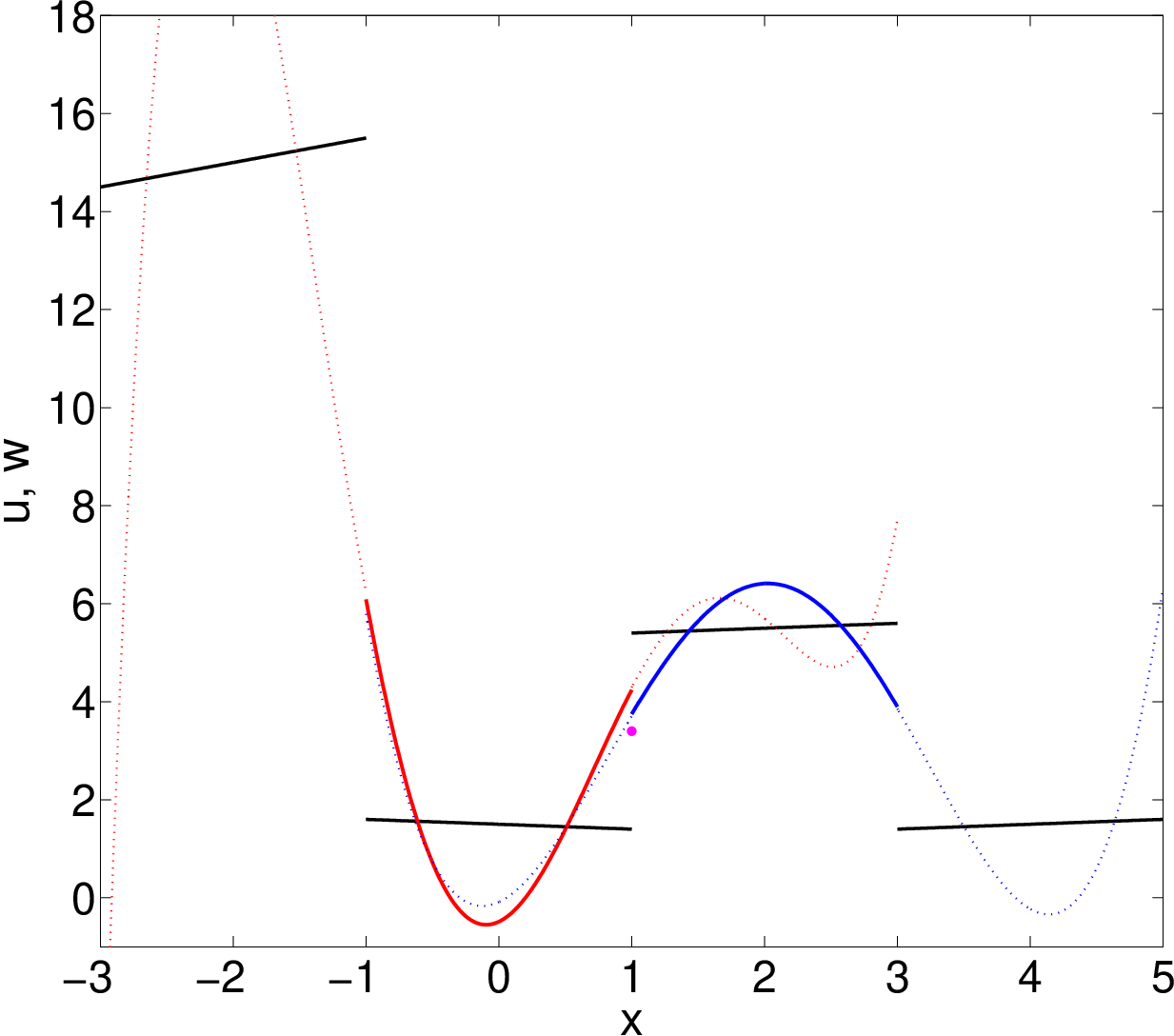
In the next section, we describe a way to stabilize the method using a flux limiter approach. Our ansatz also covers the nonlinear case.

Now that we have seen where instabilities may occur, we develop a nonlinear fix for that problem. In order to enforce a cell entropy condition, we employ a flux limiting approach. Denote by $f_{i+\frac{1}{2}}^{u},~f_{i+\frac{1}{2}}^{w}$ numerical fluxes evaluated using $u_{h}$ and $w_{h}$, respectively. Our goal is to find a limiter $\theta_{i+\frac{1}{2}}\in[0,1]$ such that the scheme with the limited flux

$$f_{i+\frac{1}{2}}=f_{i+\frac{1}{2}}^{u}+\theta_{i+\frac{1}{2}}f_{i+\frac{1}{2}}^{r},\qquad f_{i+\frac{1}{2}}^{r}=f_{i+\frac{1}{2}}^{w}-f_{i+\frac{1}{2}}^{u}$$

(19)

satisfies the entropy condition. We denote the terms that only include $u_{h}$ by

	$\displaystyle F_{i+\frac{1}{2}}^{u}$	$\displaystyle=f_{i+\frac{1}{2}}^{u}u_{i+\frac{1}{2}}^{-}-g(u_{i+\frac{1}{2}}^{-}),$
	$\displaystyle A^{(i)}=$	$\displaystyle-\left(u_{i-\frac{1}{2}}^{+}-u_{i-\frac{1}{2}}^{-}\right)f_{i-\frac{1}{2}}^{u}+g(u_{i-\frac{1}{2}}^{+})-g(u_{i-\frac{1}{2}}^{-}).$

Note that these are exactly the terms that occur in the original work of Jiang and Shu [17] and we recall that the essential point of their proof is that $A^{(i)}\geq 0$ since $f_{i-\frac{1}{2}}^{u}$ is a monotone E-flux. Moreover, let us use the standard notation for a jump at the cell interface $\left[\left[u\right]\right]_{i-\frac{1}{2}}=u_{i-\frac{1}{2}}^{+}-u_{i-\frac{1}{2}}^{-}$. Inserting (19) in (12) and rearranging terms yields:

	$\displaystyle\frac{dE^{(i)}}{dt}$	$\displaystyle+\left(F_{i+\frac{1}{2}}^{u}+\theta_{i+\frac{1}{2}}f_{i+\frac{1}{2}}^{r}u_{i+\frac{1}{2}}^{-}\right)-\left(F_{i-\frac{1}{2}}^{u}+\theta_{i-\frac{1}{2}}f_{i-\frac{1}{2}}^{r}u_{i-\frac{1}{2}}^{-}\right)$
		$\displaystyle+A^{(i)}-V^{(i)}-\theta_{i-\frac{1}{2}}\left[\left[u\right]\right]_{i-\frac{1}{2}}f_{i-\frac{1}{2}}^{r}=0$		(20)

Thus, defining a numerical entropy flux as

$$\hat{F}_{i+\frac{1}{2}}=F_{i+\frac{1}{2}}^{u}+\theta_{i+\frac{1}{2}}f_{i+\frac{1}{2}}^{r}u_{i+\frac{1}{2}}^{-},$$

the entropy condition

$$\frac{dE^{(i)}}{dt}+\hat{F}_{i+\frac{1}{2}}-\hat{F}_{i-\frac{1}{2}}\leq 0$$

is satisfied if

$$A^{(i)}-V^{(i)}-\theta_{i-\frac{1}{2}}\left[\left[u\right]\right]_{i-\frac{1}{2}}f_{i-\frac{1}{2}}^{r}\geq 0.$$

(21)

In the linear case $f(u)=\lambda u$ we have $V^{(i)}=0$ due to the orthogonality of the residual $r_{h}$ w.r.t. $\mathcal{V}_{h}$, hence the condition (21) simplifies to .

$$A^{(i)}-\theta_{i-\frac{1}{2}}\left[\left[u\right]\right]_{i-\frac{1}{2}}f_{i-\frac{1}{2}}^{r}\geq 0.$$

(22)

Note that $A^{(i)}\geq 0$ and so in the linear case we can always find a $\theta_{i-\frac{1}{2}}\in[0,1]$ that satisfies (22).

References

- [1] T. Aboiyar, E.H. Georgoulis, and A. Iske. Adaptive ADER Methods Using Kernel-Based Polyharmonic Spline WENO Reconstruction. SIAM Journal on Scientific Computing, 32:3251–3277, 2010.
- [2] D. Balsara, C. Altmann, C.D. Munz, and M. Dumbser. A sub-cell based indicator for troubled zones in RKDG schemes and a novel class of hybrid RKDG+HWENO schemes. Journal of Computational Physics, 226:586–620, 2007.
- [3] D.S. Balsera and C.W. Shu. Monotonicity perserving weighted essentially non-oscillatory schemes with increasingly high order of accuracy. J. Comput. Phys., 160:405–452, 2000.
- [4] C. C. Castro and E. F. Toro. Solvers for the high-order riemann problem for hyperbolic balance laws. Journal of Computational Physics, 227:2481–2513, 2008.
- [5] B. Cockburn, M. Luskin, C. W. Shu, and E. Suli. Enhanced accuracy by post-processing for finite element methods for hyperbolic equations. Mathematics of Computation, 72:577–606, 2003.
- [6] M. Dumbser. Arbitrary High Order Schemes for the Solution of Hyperbolic Conservation Laws in Complex Domains. Shaker Verlag, Aachen, 2005.
- [7] M. Dumbser. Arbitrary high order PNPM schemes on unstructured meshes for the compressible Navier–Stokes equations. Computers & Fluids, 39:60–76, 2010.
- [8] M. Dumbser, D. S. Balsara, E. F. Toro, and C.-D. Munz. A unified framework for the construction of one-step finite volume and discontinuous Galerkin schemes on unstructured meshes. Journal of Computational Physics, 227:8209–8253, September 2008.
- [9] M. Dumbser, A. Hidalgo, M. Castro, C. Parés, and E.F. Toro. FORCE schemes on unstructured meshes II: Non–conservative hyperbolic systems. Computer Methods in Applied Mechanics and Engineering, 199:625–647, 2010.
- [10] M. Dumbser and M. Käser. Arbitrary high order non-oscillatory finite volume schemes on unstructured meshes for linear hyperbolic systems. Journal of Computational Physics, 221:693–723, 2007.
- [11] M. Dumbser and O. Zanotti. Very high order PNPM schemes on unstructured meshes for the resistive relativistic MHD equations. Journal of Computational Physics, 228:6991–7006, 2009.
- [12] G. Gassner. Neuartige Discontinuous Galerkin Verfahren für Advektions-Diffusionsgleichungen. Technical report, Institut für Aerodynamik und Gasdynamik, Universität Stuttgar, 2004.
- [13] S.K. Godunov. Finite difference methods for the computation of discontinuous solutions of the equations of fluid dynamics. Mathematics of the USSR - Sbornik, 47:271–306, 1959.
- [14] C. R. Goetz and A. Iske. Approximate solutions of generalized Riemann problems for nonlinear systems of hyperbolic conservation laws. Math. Comp., 85:35–62, 2016.
- [15] S. Gottlieb, C.-W. Shu, and E. Tadmor. Strong Stability-Preserving High-Order Time Discretization Methods. SIAM Review, 43:89–112, January 2001.
- [16] A. Harten, B. Engquist, S. Osher, and S.R. Chakravarthy. Uniformly high order accurate essentially non-oscillatory schemes III. Journal of Computational Physics, 71:231–303, 1987.
- [17] G. Jiang and C.W. Shu. On a cell entropy inequality for discontinuous Galerkin methods. Mathematics of Computation, 62:531–538, 1994.
- [18] G.S. Jiang and C.W. Shu. Efficient implementation of weighted ENO schemes. Journal of Computational Physics, 126:202–228, 1996.
- [19] H. Luo, L. Luo, R. Nourgaliev, V.A. Mousseau, and N. Dinh. A reconstructed discontinuous Galerkin method for the compressible Navier-Stokes equations on arbitrary grids. Journal of Computational Physics, 229:6961–6978, 2010.
- [20] H. Luo, Y. Xia, S. Spiegel, R. Nourgaliev, and Z. Jiang. A reconstructed discontinuous Galerkin method based on a Hierarchical WENO reconstruction for compressible flows on tetrahedral grids . Journal of Computational Physics, 236:477–492, 2013.
- [21] S. Osher. Riemann solvers, the entropy condition and difference approximations. SIAM Journal on Numerical Analysis, 21:217–235, 1984.
- [22] J. Qiu and C.W. Shu. Hermite WENO schemes and their application as limiters for Runge-Kutta discontinuous Galerkin method: one-dimensional case. Journal of Computational Physics, 193:115–135, 2003.
- [23] J. Qiu and C.W. Shu. Hermite WENO schemes and their application as limiters for Runge-Kutta discontinuous Galerkin method II: two dimensional case. Computers and Fluids, 34:642–663, 2005.
- [24] J.K. Ryan, C.W. Shu, and H.L. Atkins. Extension of a post-processing technique for the discontinuous Galerkin method for hyperbolic equations with applications to an aeroacoustic problem. SIAM Journal on Scientific Computing, 26:821–843, 2005.
- [25] V.A. Titarev and E.F. Toro. ADER: Arbitrary high order Godunov approach. Journal of Scientific Computing, 17(1-4):609–618, 2002.
- [26] V.A. Titarev and E.F. Toro. Finite–volume WENO schemes for three–dimensional conservation laws. Journal of Computational Physics, 201:238–260, 2004.
- [27] V.A. Titarev and E.F. Toro. ADER schemes for three-dimensional nonlinear hyperbolic systems. Journal of Computational Physics, 204:715–736, 2005.
- [28] E. F. Toro and V. A. Titarev. Derivative Riemann solvers for systems of conservation laws and ADER methods. Journal of Computational Physics, 212(1):150–165, 2006.
- [29] L. Zhang, L. Wei, H. Lixin, D. Xiaogang, and Z. Hanxin. A class of hybrid DG/FV methods for conservation laws I: Basic formulation and one-dimensional systems. Journal of Computational Physics, 231:1081–1103, 2012.