Analytic approximations of neutrino luminosities and heat capacities of neutron stars with nucleon cores
Abstract
We derive analytic approximations of neutrino luminosities and heat capacities of neutron stars with nucleon cores valid for a wide class of equations of state of dense nucleon matter. The neutrino luminosities are approximated for the three cases in which they are produced by (i) direct Urca or (ii) modified Urca processes in non-superfluid matter, or (iii) neutrino-pair bremsstrahlung in neutron-neutron collisions (when other neutrino reactions are suppressed by strong proton superfluidity). The heat capacity is approximated for the two cases of (i) non-superfluid cores and (ii) the cores with strong proton superfluidity. The results can greatly simplify numerical simulations of cooling neutron stars with isothermal interiors at the neutrino and photon cooling stages as well as simulations of quasi-stationary internal thermal states of neutron stars in X-ray transients. For illustration, a model-independent analysis of thermal states of the latter sources is outlined.
Keywords:
dense matter – stars: neutron – neutrino emission – XRTs: quiescent.1 Introduction
It is well known that observations of thermal radiation from cooling (isolated) neutron stars and from accreting neutron stars in quiescent states of X-ray transients (XRTs) can be used to infer (constrain) parameters of neutron stars and explore properties of superdense matter in their interiors (e.g., Yakovlev & Haensel 2003; Yakovlev et al. 2003; Yakovlev & Pethick 2004; Page et al. 2009; Potekhin et al. 2015 and references therein). This can be done by modeling thermal states and evolution of isolated and transiently accreting neutron stars and by comparing theoretical models with observations.
In this way one can test various model equations of state (EOSs) of superdense matter in neutron star cores — whether these EOSs are consistent with the data or not. Direct numerical modeling for the different EOSs and masses of neutron stars is often time consuming and requires complicated computer codes. It is the aim of the present paper to simplify the task by obtaining analytic approximations for basic integral properties of neutron stars which determine their thermal evolution.
Specifically, we consider thermally relaxed neutron stars which are isothermal inside (e.g. Glen & Sutherland 1980). Taking into account the effects of General Relativity, they should possess spacially constant redshifted internal temperature
| (1) |
where is a local temperature of the matter and is the metric function which determines gravitational redshift. A noticeable temperature gradient persists only in a thin outer (heat blanketing) envelope with a rather poor thermal conductivity; its thickness does not exceed a few hundred meters (e.g., Gudmundsson et al. 1983; Potekhin et al. 1997). We will study redshifted integrated neutrino luminosities and heat capacities of such stars which are the main ingredients for simulating their thermal structure and evolution. These quantities are mainly determined by bulky and massive neutron star cores and depend on . They depend also on the EOS of neutron star matter and on the stellar mass . The neutrino luminosity is the sum of the luminosities provided by different neutrino emission mechanisms. Both quantities, and , can be strongly affected by superfluidity in the neutron star cores.
We study a wide class of EOSs of neutron star cores composed of neutrons, protons, electrons and muons. These EOSs may open or forbid the powerful direct Urca processes of neutrino emission in neutron star cores (Lattimer et al., 1991). We consider either non-superfluid (normal) cores or the cores with strong proton superfluidity which suppresses all neutrino processes involving protons as well as the proton heat capacity in the core (e.g. Yakovlev et al. 2001). We will calculate and and approximate them by analytic expressions which are universal for all chosen EOSs. This universality greatly simplifies theoretical analysis of observational data on cooling isolated and transiently accreting neutron stars. For illustration, we give a sketch of such an analysis for quasi-stationary neutron stars in XRTs. In our analysis we neglect possible effects of magnetic fields.
2 Cooling properties of neutron stars
Let us outline the main elements of the cooling theory of neutron stars (e.g., Yakovlev & Pethick 2004). During the first yr after their birth neutron stars cool mostly via neutrino emission from their interiors. During an initial cooling period yr the internal regions of the star become isothermal. Since then neutrinos are mainly generated in the stellar core. The basic neutrino emission mechanisms in the core are the direct Urca (DU) and modified Urca (MU) processes as well as neutrino-pair bremsstrahlung in baryon collisions. Neutrino emissivities of these processes strongly depend on the properties of the matter — on composition and superfluidity of baryons (e.g. Yakovlev et al. 2001).
In the present paper we assume that the neutron star core consists of neutrons with some admixtures of protons, electrons and muons (-matter) in beta equilibrium. The neutrino emissivities of relevant processes are reviewed, for instance, by Yakovlev et al. (2001). We will study the case of fully non-superfluid (non-SF) matter and the case of strongly superfluid (SF) protons with other particles being in normal states. The first case refers to the standard neutrino emission level and describes the so called standard neutrino candles. The main contribution to the luminosity of the neutron star core comes from the DU or MU processes. For the MU process, we have
| (2) |
where , , and are the number densities of neutrons, protons, electrons and muons, respectively; fm-3 is the standard number density of nucleons in saturated nuclear matter, is a local temperature expressed in K and is a dimensionless factor to account for different branches of the process (see, e.g., Yakovlev et al. 2001; Kaminker et al. 2016). In this work we need only the main dependence . The factor erg cm-3 s-1 is calculated under the assumptions described by Yakovlev et al. (2001), with an effective masses of protons and neutrons and , respectively.
For the DU process, we have (e.g., Yakovlev et al. 2001)
| (3) |
where erg cm-3 s-1, while the factors and are equal to (open the electron and muon processes, respectively) if Fermi momenta of reacting particles satisfy the triangle condition; otherwise, these factors are zero. Because of the triangle conditions, the electron and muon DU processes have thresholds and can operate only in the central regions of massive neutron stars. For some EOSs, they do not operate at all.
The SF case corresponds to the most slowly cooling neutron stars (e.g., Ofengeim et al. 2015), where all neutrino reactions involving protons are strongly suppressed by proton superfluidity and the most efficient neutrino emission is provided by the nn-bremsstrahlung. Then (e.g. Yakovlev et al. 2001)
| (4) |
where erg cm-3 s-1.

Another quantity important for cooling neutron stars is the specific heat of the neutron core . Since neutron stars are mainly composed of strongly degenerate particles, the heat capacities at constant volume and pressure are almost identical and we do not discriminate between them. In the non-SF case there are four contributions to the specific heat in a nucleon neutron star core,
| (5) |
For one has
| (6) |
where is the Boltzmann constant while and are, respectively, the effective mass and the Fermi momentum of particles . Note that the main contributions to comes from and (e.g., Page 1993). Taking and , we obtain
| (7) |
with n or p, and erg cm-3 K-1. In the case of very strong proton superfluidity one has .
Integration of and over the neutron star core gives the neutrino luminosity and the heat capacity of the core. The same quantities for the crust are negligible after the star reaches the state of internal thermal relaxation (e.g. Yakovlev et al. 2001; Yakovlev & Pethick 2004). If so, and are almost equal to the total neutrino luminosity and heat capacity of the star, respectively. We will perform the integration of and for different EOSs in the core assuming isothermal interior of the star.
3 Zoo of equations of state
| EOS | , M | , km | , M | , km |
|---|---|---|---|---|
| NL3 | 2.75 | 13.00 | 2.60 | 13.79 |
| PAL4-240 | 1.93 | 10.24 | 1.64 | 11.93 |
| BSk21 | 2.27 | 11.01 | 1.59 | 12.59 |
| BSk20 | 2.16 | 10.10 | — | — |
| SLy | 2.05 | 9.90 | — | — |
| APR II | 1.92 | 10.20 | 1.89 | 10.83 |
| APR IV | 2.16 | 10.82 | 1.73 | 12.48 |
| DDME2 | 2.48 | 12.05 | — | — |
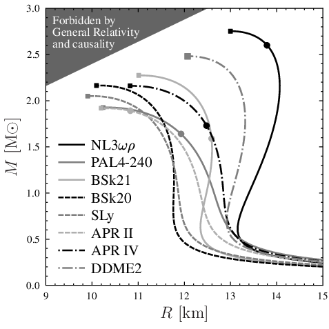
Let us take eight EOSs of superdense matter in neutron star cores. They are illustrated in Figs. 2–3. The NL3 and DDME2 EOSs are described in Fortin et al. (2016) and in references therein; the SLy EOS is taken from Douchin & Haensel (2001); PAL4-240 is the model after Page & Applegate (1992) but with a different compression modulus at saturation, MeV (see also the PAPAL model in the Appendix D of Haensel et al. 2007); the APR II EOS is introduced by Gusakov et al. (2005); the BSk20 and BSk21 EOSs are parametrized by Potekhin et al. (2013), and the APR IV EOS is constructed by Kaminker et al. (2014) (who called it the HHJ EOS). For the SLy, BSk20 and BSk21 models, the EOSs in the crust and the core are calculated in a unified way; the NL3 and DDME2 crustal parts are described by Fortin et al. (2016); for other models, the smooth composition EOS of the crust (Haensel et al., 2007) is used. The most important parameters of neutron stars for the selected EOSs are listed in Table 1.

The relations for neutron star models with these EOSs are plotted in Fig. 2. We choose the EOSs with different stiffness in order to consequently cover a large part of the plane. Squares in Fig. 2 correspond to the most massive stable neutron star models. The selected EOSs are reasonably consistent with recent discoveries of two massive () neutron stars (Demorest et al., 2010; Antoniadis et al., 2013). Circles mark configurations where the DU process becomes allowed. Only five EOSs from Table 1 open the DU process before the most massive stable configuration is reached.
In Fig. 2 we plot the relations for the selected EOSs. These relations have several common features. First, the EOSs at g cm-3 (the dotted vertical line) are not dramatically different (differences in are within a factor of 2). It is because, as a rule, the EOSs are constructed in such a way to reproduce the properties of saturated nuclear matter which are well studied in laboratory. Secondly, the stiffer the high-density EOS, the larger . Finally, in spite of the similarity of the relations near they they are sufficiently different at which results in rather different relations. The straight thick shaded strip line in Fig. 2 corresponds to a family of simple polytropic EOS models with the power-law index . It is a good overall approximation as discussed in Section 4.3.
Fig. 3 illustrates another important property of the selected EOSs, the relation between the proton and total baryon number densities. A bunch of the curves for the different EOSs is the thinnest at (the dotted vertical line). It is a consequence of the calibration of the EOSs to the standard nuclear theory. The straight thick shaded strip corresponds to the relations , which can be derived from the free-particle model at not too high (e.g., Friman & Maxwell 1979; Shapiro & Teukolsky 1983). Fig. 3 shows that this simple approximation is qualitatively accurate which is sufficient for our analysis.
Let us stress that we do not intend to accurately fit the EOSs or number densities of different particles. Our aim is to suggest some simple scaling expressions for these quantities and use them to fit the expressions for the integral quantities, such as and . One can treat these scaling expressions as purely auxiliary and phenomenological (although we prefer to introduce them on physical grounds). We will see that the integration over the core absorbs the inaccuracy of scaling expressions and enables us to accurately describe the integral quantities.
4 Integration of neutrino luminosity and heat capacity
4.1 Basic expressions
The neutrino luminosity of a neutron star core redshifted for a distant observer is given by
| (8) |
The heat capacity of the core is
| (9) |
Here is the core radius, is the gravitational mass inside the sphere of radial coordinate , and is the metric function determined by the equation (e.g. Haensel et al. 2007, Ch. 6)
| (10) |
The neutrino emissivity and the specific heat are expressed here as functions of the local temperature and the local density . In a star with isothermal interiors is given by equation (1), , with being constant over the isothermal region.
Let us analyse three cases of neutrino emission in equation (8). The first is the SF case, where is given by equation (4). The second is the non-SF case with the forbidden DU process, so that , equation (2). The third case is also for the non-SF core but with the allowed DU process. In this case, we set , given by equation (3). To simplify our analysis, in this paper we use throughout the entire neutron star core (to avoid complications associated with the introduction of the DU threshold). This simplification is qualitatively justified because, typically, , and even a small central kernel with the allowed DU process makes drastically larger than . However, it somewhat overestimates and gives only its firm upper limit.
4.2 Analytic approximations of the integrals
Exact analytic integration in equations (8) and (9) is not possible. Instead, we derive approximate expressions for these integrals and calibrate them using the results of numerical integration.
Because the mass of a neutron star crust is typically about 1 per cent of the total mass , we can safely set that and , where
| (11) |
It is convenient to introduce .
To proceed further we need approximate expressions for the number densities of particles in neutron star cores. Let us assume that the main contribution to the baryon number density is provided by neutrons, and the number densities of charged particles are described by the model similar to the free-particle one,
| (12) |
Here is a dimensionless constant which can be treated as a value averaged over the all selected EOSs. The relation can be taken from Haensel et al. (2007, Ch. 6),
| (13) |
being the rest mass per baryon in the 56Fe nucleus.
The approximate equality in equation (12) can be significantly violated at very high densities where . Such densities occur near the centers of massive neutron stars; their contribution to the integrated neutrino luminosities and heat capacities is small, except for , where the contributions of the muon and electron DU processes are equal.
As mentioned above, we study the three scenarios (nn, MU and DU) of neutrino emission in equation (8). In the first (nn) case we take from equation (4). In the second (MU) case we employ from equation (2), but we will additionally simplify it assuming . In the third (DU) case we use equation (3) but replace the sum of -functions by a factor . Since typical densities, where the DU processes operate, are so high that muons appear, such a simplification is reasonable.
Considering the specific heat, we use the approximation (7), , with different constants for the non-SF and SF cases.
Let us factorize (8) and (9) into dimensional and dimensionless terms. It is convenient to define
| (14a) | |||
| (14b) | |||
| (14c) |
We assume that has a universal form for any EOS, and of our study. According to Lattimer & Prakash (2001), such an approximation is reasonable. Then equation (8) yields
| (15) |
where ; , and for the nn-bremsstrahlung; , and for the MU process; , and for the DU process; In equation (15) we have introduced a dimentionless constant to absorb the inaccuracy of due to our approximations of and in the DU and MU cases; in the SF case . Similarly, for the heat capacity (9) we obtain
| (16) |
where constants are different in the SF and non-SF cases.
Next consider a polytropic EOS, , with some effective whose value will be obtained later by calibrating to numerical calculations of and . Then we analytically derive from equation (10) with the condition ,
| (17) |
where and are, respectively, the density and pressure at the core-crust interface. Actually, this solution behaves as
| (18) |
At the next step we stress that the ratio only slightly varies for different stellar masses higher than . Thus we assume to be constant in Eqs. (15) and (16). Then, combining equations (14b) and (18) with (15) and (16), we see that the integrals are parametrised by and . All uncertainties of calculations of the integrals are encapsulated in the functions and . These functions should be smooth as proven by (14). Thus the dependence of the integrals in equations (15) and (16) on and can be understood using the midpoint method, by taking the integrands at some fixed value of x between and , . For simplicity, we assume that this value is independent of and . It is convenient to introduce
| (19) |
Then the final expressions for the neutrino luminosity and heat capacity take the forms
| (20) |
Here we use instead of because is taken to be constant in our analytic models and the difference is absorbed in fit parameters described below. The exponents , and are taken from equations (15) and (16) and listed in Table 2. The dimensionless parameters , , and the most suitable values of in (19) will be obtained by the calibration to numerical calculations.
4.3 Calibration to numerical calculations
| or | Case | or | rms | max error | |||||||
|---|---|---|---|---|---|---|---|---|---|---|---|
| nn (SF) | erg cm-3 s-1 | 8 | 1 | 6 | 2.03 | 1.14 | 0.0047 | 2.51 | 0.14 | 0.54 at NL3 | |
| MU (non-SF) | erg cm-3 s-1 | 8 | 2 | 6 | 1.12 | 1.14 | 0.0060 | 2.45 | 0.25 | 0.66 at NL3 | |
| DU (non-SF) | erg cm-3 s-1 | 6 | 2 | 4 | 1.01 | 1.14 | 0.0031 | 2.48 | 0.16 | 0.40 at NL3 | |
| non-SF | erg cm-3 K-1 | 1 | 1 | 1 | 2.68 | 1.14 | 0.0174 | 2.11 | 0.05 | 0.12 at BSk20 | |
| SF | erg cm-3 K-1 | 1 | 1 | 1 | 2.01 | 1.06 | 0.0159 | 2.18 | 0.05 | 0.09 at NL3 |


The integrals (8) and (9) have been calculated numerically. In this way we have obtained accurate values of and for any selected EOS, any scenario (nn, MU, DU, SF, non-SF) and for a range of masses . In the calculations, we have used the expressions for and described in Sections 2 and 4.1. As mentioned above, while calculating we have extended over the entire neutron star core. However, for the DU case we have not used stellar models with M because M for all our models (Table 1).
Our numerical results are shown by different symbols in Fig. 4. These data have been used to calibrate our analytic approximation (20). We have obtained 109 values of the neutrino luminosity (cases nn and MU, excluding DU) as well as 109 values of the heat capacity (cases SF and non-SF). For the DU case we have excluded 40 values with M. The trial fuctions and (equations (19), (20)) have been calibrated to these data sets. The target fuction to minimize has been the relative root mean square (rms) error. The optimised values of , , and as well as the corresponding fit errors are listed in Table 2. The obtained approximations are also plotted on Fig. 4.
Let us discuss the approximations of . They are most precise for the nn-bremsstrahlung; the rms errors appear the smallest because is independent of the fractions of charged particles in dense matter. However, it has large maximal relative error which occurs for the most massive star with the NL3 EOS. This is because the approximation of this EOS by a single polytrope does not reproduce well its high density behaviour. The largest errors occur for the MU case due to a strong dependence of on the fractions of charged particles through the factor . The approximation of is more accurate than the approximation of because depends on in a rather simple way.
The importance of charged particle fractions can be demonstrated by instructive examples of the BSk20 and APR IV EOSs. In Figs. 2–4 the corresponding curves are plotted by short-dashed (BSk20) and dot-dashed (APR IV) lines. The initial numerical data in Fig. 4 are displayed by black squares (BSk20) and triangles (APR IV). According to Fig. 2, these EOSs have very close maximum masses, but the stars with the BSk20 EOS are more compact, i.e. have smaller radii than the APR IV stars of the same . Roughly speaking, the relations for these EOSs differ by a shift along the axis. This means that a BSk20 star is denser than an APR IV star, and, therefore, has larger . This is true for (Fig. 4): black squares (for BSk20) lie higher than black triangles (for APR IV). This feature is well reproduced by the black dashed and dot-dashed lines, which show the approximation (20) for these EOSs. In contrast, the MU and DU luminosities are sensitive to the relations. According to Fig. 3, the values of for the APR IV EOS are noticeably higher than for the BSk20 EOS. The opposite effects of the two factors, the greater compactness of the BSk20 stars and the larger for the APR IV stars, leads to their compensation. Accordingly, the DU as well as the MU neutrino luminosities for these EOSs appear to be close enough (triangles and black squares on the left-hand panel of Fig. 4 overlap). Because the approximation (20) is derived using not very accurate description of proton, electron and muon fractions, it cannot reproduce this effect exactly; an approximate expression gives and higher than numerical values for the BSk20 EOS and lower than for the APR IV EOS.
Another interesting note is that the parameter of our approximation takes very close values for the non-SF (DU and MU) cases but is several times larger for the SF (nn-bremsstrahlung) case. This is because should include the value from (12) and the extra factor in the non-SF case but not in the SF case. Because both these factors are smaller than 1, the value of should be several times lower in the non-SF case than in the SF one, in agreement with Table 2.
Now let us outline the approximations of the heat capacity (the right-hand side of Fig. 4). The different EOSs give so close values of , that the approximation (20) hardly resolves them. Note that the parameters , and , which determine the relation, are similar in the SF and non-SF cases. This supports the idea that the behavior of the total specifiec heat is similar to that of in both these cases. A difference between the values of shows that switching off the proton contribution by superfluidity just reduces the heat capacity by about 25 per cent, in agreement with the results by Page (1993).
Let us mention several common features of our approximations. First, we can see that the index ranges from about 2.1 to 2.5 with the average value . Such a polytropic EOS is plotted in Fig. 2 by a thick green line and is in good agreement with the selected EOSs. Secondly, the largest errors occur at the maximum neutron star masses, because the higher the density the stronger the difference between the EOS models. Thirdly, the fact that the maximum errors occur for the NL3and BSk20 EOSs is explained by the largest deviations of (NL3) and (BSk20) relations from the average trend (Fig. 3).
It is also remarkable that at low the exact dependence is insensitive to an EOS. This gives hope to derive this dependence analytically for which is out the scope of the present work.
5 Quiescent states of XRTs
For illustration, we apply our approximations of to analyse transiently accreting neutron stars in XRTs (low-mass X-ray binaries). The formalism of applying the neutron star cooling theory for exploring quasi-stationary thermal states of such objects in quiescence is well known (e.g. Yakovlev et al. 2003; Levenfish & Haensel 2007, also see Yakovlev & Pethick 2004). We will show that our approximations of simplify an analysis of observations.
5.1 Formalism of thermal states
Let us outline the main features of thermal quasi-stationary equilibrium of neutron stars in XRTs. During active states of such a source, the neutron star accretes from its low-mass companion. The accreted matter is compressed under the weight of newly accreted material. It looks as if the accreted matter sinks into deeper layers of the neutron star crust. This initiates nuclear transformations of the accreted matter accompanied by the deep crustal heating (Haensel & Zdunik, 1990; Haensel & Zdunik, 2003; Haensel & Zdunik, 2008) with the energy release of about MeV per one accreted nucleon distributed mainly in the inner crust. This deep crustal heating can be sufficiently strong to warm up old transiently accreting stars and support their observable thermal radiation during quiescent states of XRTs (Brown et al., 1998).
We will not consider the episodes of rather long or intense accretion when the deep heating is too intense and destroys thermal equilibrium between the crust and the core (e.g. Degenaar et al. 2015 and references therein). We will restrict our analysis to weaker or shorter accretion episodes. Then the stellar interior remains isothermal and quasi-stationary. On average, this heating is balanced by the thermal emission of photons from the stellar surface and neutrinos from the stellar interior. In an observer rest frame one has the thermal balance of the form
| (21) |
where
| (22) |
is the redshifted photon luminosity of the star as a function of the local effective surface temperature , and ( is defined in equation (11)), is the neutrino luminosity (8) approximated by equation (20), and
| (23) |
is the integrated rate of the energy release due to deep crustal heating. The mass accretion rate has to be averaged over the neutron star cooling time scales, and erg s-1 is consistent with the deep crustal heating rate (1.5 MeV per nucleon) given above.
Using equations (21)—(23) one can calculate and plot the neutron star heating curves in the plane (e.g., Yakovlev & Pethick 2004; Levenfish & Haensel 2007). Here we consider the two limiting cases: (i) the photon cooling regime at and (ii) the neutrino cooling regime at .
In the case (i) one has a simple relation
| (24) |
It slightly depends on and due to General Relativity effects.
In the case (ii) the relation between and is more complicated. One can use the approximations (20) to derive analytically for the three neutrino emission mechanisms, nn-bremsstrahlung in the SF case; MU or DU processes in the non-SF case (Section 4.2). Then the neutron star thermal equilibrium reads
| (25) |
, , and are listed in Table 2 for each neutrino emission scenario. To calculate one needs to relate and . This can be done using the relations derived by Potekhin et al. (2003), where is the temperature at the bottom of the neutron star heat blanketing envelope. Making use of and equation (25), we obtain
| (26) |
The relations are sensitive to the chemical composition of the heat blanketing envelope which is rather uncertain and depends on details of nuclear burning in the envelope. The envelope can be almost purely iron if all the accreted material has burnt to iron during an active XRT state. Alternatively, it can be almost fully accreted or intermediate if the burning in the envelope is slower. We consider the two limiting cases, the case of non-accreted iron (Fe) envelope and the case of fully accreted (acc) envelope. We denote the corresponding relations as . Using equation (22) we have
| (27) |
where ‘acc’ or ‘Fe’ while is given by equation (26).
5.2 Model-independent analysis of thermal states
| Num. | Source | Num. | Source |
|---|---|---|---|
| 1 | 4U 1608–522 | 13 | NGC 6440 X-1 |
| 2 | Aql X-1 | 14 | SAX J1810.8–2609 |
| 3 | 4U 1730–22 | 15 | MXB 1659–29 |
| 4 | RX J1709–2639 | 16 | IGR 00291+5934 |
| 5 | Terzan 5 | 17 | XTE J1814–338 |
| 6 | 4U 2129+47 | 18 | XTE J2123–058 |
| 7 | 1M 1716–315 | 19 | XTE J1807–294 |
| 8 | Terzan 1 | 20 | XTE J0929–314 |
| 9 | 2S 1803–45 | 21 | EXO 1747–214 |
| 10 | KS 1731–260 | 22 | NGC 6440 X-2 |
| 11 | Cen X-4 | 23 | 1H 1905+000 |
| 12 | XTE J1751–305 | 24 | SAX J1808.4–3658 |

The approximations (20) and (21) greatly simplify an analysis of thermal states of neutron stars in XRTs. Now we need only mass , radius , the neutrino emission scenario and the heat blanketing envelope type to calculate an relation.
The left-hand panel of Fig. 5 shows six families of curves for a fixed time-averaged mass accretion rate M yr-1. The families are for the three scenarios of neutrino emission (nn, MU, DU) and the two limiting models of neutron star heat blanketing envelopes (Fe and acc). The curves of different types are calculated from (27) for the different EOSs (Table 1) using the appropriate relations (Fig. 2). The six horizontal shaded bands enclose the curves of these six families. Recall that the DU curves are plotted only at M, moreover, even at M the DU curves are only underestimations of relations, as our approximations overestimate . The presented bands can be treated as overestimated photon thermal luminosity bands for the DU curves. For each band, the bounding stellar models are chosen as M, km (SLy; lower bound) and M, km (NL3; upper bound).
Note that the relations are mostly non-monotonic. The luminosity increases with growing for low-mass stars but then decreases again for massive stars; the lowest does not necessarily correspond to the brightest source in the band. This is a consequence of General Relativity effects.
The right-hand panel of Fig. 5 shows the same six bands as on the left-hand panel, but in the plane. Thin curves present numerical solutions of the initial equation (21) (without assuming ) for the bounding neutron star models (see above). Such solutions almost coincide with the approximate ones if . We stress that Fig. 5 illustrates only six representative scenarios of thermal states of neutron stars. Any filled band limits possible values of versus or for neutron stars with the selected EOSs. Although the set of these EOSs is restricted we expect that the bands are robust (should not be greatly changed for a wider class of EOSs of nucleon matter). Another important feature is that the direct effect of the EOS on thermal states of neutron stars in XRTs for any of the six scenarios does not seem very strong. Therefore, the analysis of these scenarios is relatively model-independent.
Note also that the thin theoretical curves are valid only at M yr-1. At higher accretion rates the internal thermal equilibrium of the neutron star is violated. This leads to higher than predicted by isothermal calculations.
The theoretical bands on the right-hand panel of Fig. 5 are compared with observational data (or observational upper limits shown by arrows) for 24 sources. The data are the same as those presented by Beznogov & Yakovlev (2015a); Beznogov & Yakovlev (2015b) (who gave also the list of original publications). The sources are numbered in accordance with Table 3. They are mainly located between the MU and DU-cooling bands. Note the absence of any source with measured M yr-1 except for 4U 2129+47 (source 6) and KS 1731–260 (source 10), for which only upper limits are given.
The thick solid black line on the right-hand panel of Fig. 5 corresponds to (for non-redshifted quantities, ). It is the absolute upper bound on the thermal quiescent luminosity of a neutron star in the deep crustal heating scenario. One can see that all the data satisfy this upper bound. Actually, the data agree also with the highest ‘nn acc’ band and even with lower ‘MU acc’ or ‘nn iron’ bands, but disagree with the ‘MU iron’ band. This means that all the hottest neutron stars observed in quescent states of XRTs cannot be explained by the standard MU neutrino cooling and the standard iron envelopes. One needs either a slower (nn) neutrino cooling (strong SF) and/or accreted envelopes to raise and explain the data. The possibility of raising by strong SF has been analysed earlier (e.g., Yakovlev & Pethick 2004).
While the direct effects of EOS on thermal states of neutron stars in XRTs are not strong, other factors are seen (Fig. 5) to affect these thermal states much stronger. For instance, fixing the neutrino emission scenario (nn, MU or DU) but varying chemical composition of the heat blanketing envelope from pure iron to pure accreted can produce much stronger variations of (much wider bands) than those due to the EOSs. Alternatively, fixing the envelope composition (Fe or acc) and varying the neutrino emission scenarios (from nn to MU by proton superfluidity and to DU either by superfluidity or by nuclear physics effects, which shift ), one can produce even stronger variations of .
Recall that in the strong neutrino emission (DU) scenario we have artificially extended the operation of the DU process over the entire neutron star core overestimating in massive stars. Accordingly, our DU bands in Fig. 5 appear to be downshfted by a factor of few with respect to the heating curves calculated in the previous analyses (e.g., Yakovlev et al. 2003; Levenfish & Haensel 2007; Beznogov & Yakovlev 2015a; Beznogov & Yakovlev 2015b). Therefore, one should be careful in using our DU bands for analysing thermal states of the coldest sources, 1H 1905+000 (Jonker et al., 2006; Jonker et al., 2007; Heinke et al., 2009) and SAX J1808.4–3658 (Heinke et al., 2007; Tomsick et al., 2005; Jonker et al., 2004) as massive neutron stars with the DU process on. These sources are very important for proving (or disproving) the operation of the DU process in massive stars. The real DU bands should lie by a factor of higher (in natural scale). However, we believe that our current DU bands have realistic widths and reasonably well describe variations of due to composition of the envelopes. We expect to improve our model-independent analysis of the DU bands in our future publication.
6 Discussion and conclusions
We have considered a representative set of seven EOSs for neutron stars with nucleon cores (Table 1) and analysed the models of neutron stars with isothermal interiors (with constant redshifted internal temperatures ). We have calculated the neutrino luminosities and heat capacities of the cores of these stars with masses for several important scenarios of neutron star internal structure. The quantities and almost coincide with the total neutrino luminosities and heat capacities of neutron stars.
Specifically, we have studied the three scenarios for which correspond to (i) the neutrino-pair bremsstrahlung in nn collisions (owing to the presence of strong proton superfluidity in the core); (ii) non-SF stars which cool via MU processes; (iii) non-SF stars cooling via powerful DU processes. We have considered the two scenarios for , relevant for non-SF cores and the cores with strong proton superfluidity. The calculated values of and have been accurately fitted by the analytic expressions (20) which are universal for all selected EOSs. The fit parameters (Table 2) are almost independent of the specific EOS. We expect that and calculated for neutron stars with other EOSs of nucleon matter would be similar and could be approximated in the same way making our approximations almost model independent.
In this sense our consideration extends model-independent analysis of cooling neutron stars based on the standard neutrino cooling function (Yakovlev et al., 2011; Weisskopf et al., 2011; Klochkov et al., 2015; Ofengeim et al., 2015). Ofengeim et al. (2015) derived also model-independent approximations to the neutrino cooling function for stars with strong proton superfluidity. Shternin & Yakovlev (2015) performed a more complicated model-independent analysis of the cooling enhanced by the onset of triplet-state pairing of neutrons and associated neutrino emission in neutron star cores.
Our present results are more refined because we analyse a weak dependence of and on the EOS. Our approximations of and greatly simplify calculations of cooling of isolated neutron stars at the neutrino cooling stage after the initial thermal relaxation ( yr). This cooling is governed by the neutrino cooling function . The expressions for obtained from our fits of and are in good agreement with the approximations used in Yakovlev et al. (2011); Weisskopf et al. (2011); Klochkov et al. (2015); Ofengeim et al. (2015) but ours seem more complete. The approximations of should simplify cooling simulations of isolated neutron stars at the photon cooling stage (at yr, when the neutrino luminosity becomes unimportant). Finally, the approximations we obtained for simplify considerations of thermal states of accreting neutron stars in quasi-stationary XRTs as demonstrated in Section 5.
Let us stress that our results are far from being perfect because they are obtained under a number of simplified assumptions. For instance, while constructing the approximations we have assumed the ratio to be constant. In fact, it slightly decreases with the growth of . It may be so that one can improve our fits taking into account the approximations of by Zdunik et al. (2016).
While approximating we have assumed that the DU process is open in the entire core. In fact, it can operate in a small central kernel. The size of this kernel depends on and the EOS model. Its radius is zero at but increases with growing . Moreover, according to Table 1, for three of the seven selected EOSs the DU process is forbidden in all stable neutron star models. Thus, our approximation of can be treated as an overestimation to be improved in the future.
We have considered superfluidity of nucleons in a simplified manner, i.e. we have assumed that neutrons are totally non-superfluid but protons are either totally non-superfluid or fully superfluid. The advantages and disadvantages of such a treatment are discussed by Ofengeim et al. (2015).
Another simplification of our approach is in using constant effective nucleon masses equal to 0.7 of their bare masses. In addition, the neutrino emissivities have been calculated employing approximate squared matrix elements of neutrino reactions taken by Yakovlev et al. (2001) from calculations by Friman & Maxwell (1979). We expect that we can include a more advanced physics using a similar formalism when this physics appears for a number of representative EOSs.
Acknowlegements
The work of DG was supported partly by the RFBR (grants 14-02-00868-a and 16-29-13009-ofi-m) and the work of PH, LZ and MF by the Polish NCN research grant no. 2013/11/B/ST9/04528. One of the authors (DDO) is grateful to N. Copernicus Astronomical Center for hospitality and perfect working conditions.
References
- Antoniadis et al. (2013) Antoniadis J., Freire P. C. C., Wex N., Tauris T. M., Lynch R. S., van Kerkwijk M. H., et al. 2013, Science, 340, 448
- Beznogov & Yakovlev (2015a) Beznogov M. V., Yakovlev D. G., 2015a, MNRAS, 447, 1598
- Beznogov & Yakovlev (2015b) Beznogov M. V., Yakovlev D. G., 2015b, MNRAS, 452, 540
- Brown et al. (1998) Brown E. F., Bildsten L., Rutledge R. E., 1998, Atrophys. J. Lett., 504, L95
- Degenaar et al. (2015) Degenaar N., Wijnands R., Bahramian A., Sivakoff G. R., Heinke C. O., Brown E. F., Fridriksson J. K., Homan J., Cackett E. M., Cumming A., Miller J. M., Altamirano D., Pooley D., 2015, MNRAS, 451, 2071
- Demorest et al. (2010) Demorest P. B., Pennucci T., Ransom S. M., Roberts M. S. E., Hessels J. W. T., 2010, Nature, 467, 1081
- Douchin & Haensel (2001) Douchin F., Haensel P., 2001, Astron. Astrophys., 380, 151
- Fortin et al. (2016) Fortin M., Providencia C., Raduta A. R., Gulminelli F., Zdunik J. L., Haensel P., Bejger M., 2016, ArXiv e-prints
- Friman & Maxwell (1979) Friman B. L., Maxwell O. V., 1979, Astrophys. J., 232, 541
- Glen & Sutherland (1980) Glen G., Sutherland P., 1980, Astrophys. J., 239, 671
- Gudmundsson et al. (1983) Gudmundsson E. H., Pethick C. J., Epstein R. I., 1983, Astrophys. J., 272, 286
- Gusakov et al. (2005) Gusakov M. E., Kaminker A. D., Yakovlev D. G., Gnedin O. Y., 2005, MNRAS, 363, 555
- Haensel et al. (2007) Haensel P., Potekhin A. Y., Yakovlev D. G., 2007, Neutron Stars. 1. Equation of State and Structure. Springer, New York
- Haensel & Zdunik (1990) Haensel P., Zdunik J. L., 1990, Astron. Astrophys., 227, 431
- Haensel & Zdunik (2003) Haensel P., Zdunik J. L., 2003, Astron. Astrophys., 404, L33
- Haensel & Zdunik (2008) Haensel P., Zdunik J. L., 2008, Astron. Astrophys., 480, 459
- Heinke et al. (2009) Heinke C. O., Jonker P. G., Wijnands R., Deloye C. J., Taam R. E., 2009, Astrophys. J., 691, 1035
- Heinke et al. (2007) Heinke C. O., Jonker P. G., Wijnands R., Taam R. E., 2007, Astrophys. J., 660, 1424
- Jonker et al. (2006) Jonker P. G., Bassa C. G., Nelemans G., Juett A. M., Brown E. F., Chakrabarty D., 2006, MNRAS, 368, 1803
- Jonker et al. (2007) Jonker P. G., Steeghs D., Chakrabarty D., Juett A. M., 2007, Astrophys. J. Lett., 665, L147
- Jonker et al. (2004) Jonker P. G., Wijnands R., van der Klis M., 2004, MNRAS, 349, 94
- Kaminker et al. (2014) Kaminker A. D., Kaurov A. A., Potekhin A. Y., Yakovlev D. G., 2014, MNRAS, 442, 3484
- Kaminker et al. (2016) Kaminker A. D., Yakovlev D. G., Haensel P., 2016, Astrophys. Sp. Sci., 361, 267
- Klochkov et al. (2015) Klochkov D., Suleimanov V., Pühlhofer G., Yakovlev D. G., Santangelo A., Werner K., 2015, Astron. Astrophys., 573, A53
- Lattimer et al. (1991) Lattimer J. M., Pethick C. J., Prakash M., Haensel P., 1991, Physical Review Letters, 66, 2701
- Lattimer & Prakash (2001) Lattimer J. M., Prakash M., 2001, Astrophys. J, 550, 426
- Levenfish & Haensel (2007) Levenfish K. P., Haensel P., 2007, Astrophys. Sp. Sci., 308, 457
- Ofengeim et al. (2015) Ofengeim D. D., Kaminker A. D., Klochkov D., Suleimanov V., Yakovlev D. G., 2015, MNRAS, 454, 2668
- Page (1993) Page D., 1993, in Guidry M. W., Strayer M. R., eds, Nuclear Physics in the Universe The Geminga neutron star: Evidence for nucleon superfluidity at very high density. pp 151–162
- Page & Applegate (1992) Page D., Applegate J. H., 1992, Astrophys. J. Lett., 394, L17
- Page et al. (2009) Page D., Lattimer J. M., Prakash M., Steiner A. W., 2009, Astrophys. J., 707, 1131
- Potekhin et al. (1997) Potekhin A. Y., Chabrier G., Yakovlev D. G., 1997, Astron. Astrophys., 323, 415
- Potekhin et al. (2013) Potekhin A. Y., Fantina A. F., Chamel N., Pearson J. M., Goriely S., 2013, Astron. Astrophys., 560, A48
- Potekhin et al. (2015) Potekhin A. Y., Pons J. A., Page D., 2015, Space Sci. Rev., 191, 239
- Potekhin et al. (2003) Potekhin A. Y., Yakovlev D. G., Chabrier G., Gnedin O. Y., 2003, Astrophys. J., 594, 404
- Shapiro & Teukolsky (1983) Shapiro S. L., Teukolsky S. A., 1983, Black holes, white dwarfs, and neutron stars: The physics of compact objects. Wiley-Interscience, New York
- Shternin & Yakovlev (2015) Shternin P. S., Yakovlev D. G., 2015, MNRAS, 446, 3621
- Tomsick et al. (2005) Tomsick J. A., Gelino D. M., Kaaret P., 2005, Astrophys. J., 635, 1233
- Weisskopf et al. (2011) Weisskopf M. C., Tennant A. F., Yakovlev D. G., Harding A., Zavlin V. E., O’Dell S. L., Elsner R. F., Becker W., 2011, Astrophys. J., 743, 139
- Yakovlev & Haensel (2003) Yakovlev D. G., Haensel P., 2003, Astron. Astrophys., 407, 259
- Yakovlev et al. (2011) Yakovlev D. G., Ho W. C. G., Shternin P. S., Heinke C. O., Potekhin A. Y., 2011, MNRAS, 411, 1977
- Yakovlev et al. (2001) Yakovlev D. G., Kaminker A. D., Gnedin O. Y., Haensel P., 2001, Phys. Rep., 354, 1
- Yakovlev et al. (2003) Yakovlev D. G., Levenfish K. P., Haensel P., 2003, Astron. Astrophys., 407, 265
- Yakovlev & Pethick (2004) Yakovlev D. G., Pethick C. J., 2004, Annu. Rev. Astron. Astrophys., 42, 169
- Zdunik et al. (2016) Zdunik J. L., Fortin M., Haensel P., 2016, in prep., Astron. Astrophys.