Conditionally Max-stable Random Fields
based on log Gaussian Cox Processes
Abstract
We introduce a class of spatial stochastic processes in the max-domain of attraction of familiar max-stable processes. The new class is based on Cox processes and comprises models with short range dependence. We show that statistical inference is possible within the given framework, at least under some reasonable restrictions.
Keywords: conditionally max-stable process; Cox extremal process; log Gaussian Cox process; mixed moving maxima; non-parametric intensity estimation
2010 MSC: Primary 60G70, 60G55
Secondary 60G60
1 Introduction
Probabilistic modelling of spatial extremal events is often based on the assumption that daily observations lie in the max-domain of attraction of a max-stable random field which justifies statistical inference by means of block maxima procedures. This methodology is applied in various branches of environmental sciences, for instance, heavy precipitation (Cooley, 2005), extreme wind speads (Engelke et al., 2015; Genton et al., 2015; Oesting et al., 2015) and forest fire danger (Stephenson et al., 2015).
At the same time modelling extreme observations on a smaller time scale is a much more intricate issue and to date only few non-trivial processes are known to lie in the max-domain of attraction (MDA) of familiar max-stable processes. Among them -stable processes (Samorodnitsky and Taqqu, 1994) form a natural class which may be rich enough to cover a wide range of environmental sample path behaviour (Stoev and Taqqu, 2005) and scale mixtures of Gaussian processes with regularly varying scale, are known to lie in the domain of attraction of extremal t-processes (Opitz, 2013). However, stable processes are themselves complicated objects whose statistical inference is a challenging research topic (Nolan, 2016) and scale mixtures of Gaussian processes have an unnatural degree of long-range dependence.
Our objective in this article is to introduce another class of spatial processes in the MDA of familiar max-stable models, which encompasses processes with short-range dependence and to explore whether statistical inference on them is feasible, at least under some reasonable restrictions.
It is well-understood that max-stable processes can be built from Poisson point processes (de Haan, 1984; Giné et al., 1990; Stoev and Taqqu, 2006). In order to define our new class of models, we modify the underlying Poisson point process such that its intensity function is no longer fixed, but may depend on some spatial random effects. We pursue this idea by introducing conditionally max-stable processes based on Cox processes (Cox, 1955) which naturally generalize the class of mixed moving maxima processes (Smith, 1990; Schlather, 2002; Zhang and Smith, 2004; Stoev, 2008). Section 2 contains the definition of our proposed model. A functional convergence theorem shows that these processes lie in the MDA of familiar mixed moving maxima processes. From a practical point of view, we choose to model the spatial random effects that influence the intensity function by a log Gaussian random field which makes the theory and application of log Gaussian Cox processes conveniently available for our setting, cf. Møller et al. (1998); Møller and Waagepetersen (2004); Møller and Schoenberg (2010); Diggle et al. (2013).
For statistical inference we take a closer look at two important aspects in the recovery of the underlying Gaussian process. In Section 4, we deal with non-parametric estimation of realizations of the random intensity of the Cox process from observations of the conditionally max-stable processes and their storm centres. Based on the outcome of this procedure, we consider parametric estimation of the covariance function of the Gaussian process in Section 5. The performance of these procedures is examined in Section 6 in a simulation study. To this end, we discuss in Section 3 how exact simulation of our proposed model can be traced back to exact simulation of max-stable random fields as in Schlather (2002). Tables, proofs and auxiliary results are postponed to the Appendix A.
2 Model specification
In this section we define our proposed model and study its properties. Since random measures and point processes are the building blocks for max-stable processes as well as our conditional model, we briefly review conventions based on Daley and Vere-Jones (2003); Daley and Vere-Jones (2008) in Appendix A.2.
Reminder on Cox processes. The following point processes are relevant for our setting. A Poisson (point) process with directing measure is a point process which satisfies that for any Borel set with the number of points in the region is Poisson distributed with parameter , i.e. and, secondly, that the random variables are jointly independent for disjoint Borel sets in . We say is a Cox process directed by the random measure and write if, conditional on , it is a Poisson process, i.e. . By definition, Poisson processes are special cases of Cox processes with deterministic directing measure which coincides with their intensity measure, that is for Borel sets and . For Cox processes, we have instead.
The following lemma may be regarded as a central limit theorem for Cox processes and will be useful for our work. It means that the superposition of i.i.d. copies of an -thinned Cox process converges weakly to a Poisson process and is an immediate consequence of Theorem 11.3.III in Daley and Vere-Jones (2008).
Lemma 1.
Let , for be a triangular array of Cox processes. Then
Definition of Cox extremal processes. Let be a (possibly deterministic) non-negative stochastic process on that we call storm process or shape. We assume to have continuous sample paths. Based on its law (on the complete separable metric space with the usual Fréchet metric) and another non-negative stochastic process on , to be called spatial intensity process, and a positive scaling constant , we define a random field on by
| (2.1) |
where is a Cox-process on , directed by the random measure
| (2.2) |
The randomness of the measure is due to the randomness of the spatial intensity process . Similarly to the situation with mixed moving maxima processes (Smith, 1990; Zhang and Smith, 2004; Stoev, 2008) or, more generally, extremal shot noise (Serra, 1984; Jourlin et al., 1988; Heinrich and Molchanov, 1994; Dombry, 2012), we will think of the processes as being random storms centred around that will affect its surroundings with severity . In case, the intensity process is almost surely identically one (), the construction of is indeed the usual mixed moving maxima process
| (2.3) |
where is the Poisson process on with directing measure
Note that, conditional on its intensity process , the extremal process is a (non-stationary) max-stable mixed moving maxima process. In the sequel, we call a conditionally max-stable random field or Cox extremal process.
2.1 Properties of Cox extremal processes
Continuity, Stationarity and Max-Domain of Attraction.
Even though the Cox extremal process in (2.1) itself is not max-stable, we show in this section that it lies in the max-domain of attraction of an associated mixed moving maxima random field under rather general conditions.
To show this, we first clarify some technical requirements that guarantee the finiteness and the continuity of sample paths of and .
Lemma 2 (Finiteness and Sample-Continuity).
Let be a (not necessarily compact) subset of .
- (a)
If the integrability condition
(2.4) holds, then is almost surely finite.
- (b)
If, additionally,
(2.5) then the sample paths of the process are almost surely continuous on .
- (c)
Remark 3.
The Cox extremal process is in general not uniquely determined by the choice of its shape and intensity process . For instance, let be a process which satisfies the same assumptions as , and independently of , let be a random variable, such that can be decomposed into
Then choosing as shape and as intensity process does not alter the finite dimensional marginal distributions of the Cox extremal process , since
In the sequel, we will always assume that the intensity process has continuous sample paths, is strictly stationary and almost surely strictly positive with
| (2.6) |
where denotes the origin. These assumptions simplify some requirements of the preceding lemma. For instance, by Tonelli’s theorem, condition (2.4) will be equivalent to
| (2.7) |
For , we obtain that
| (2.8) |
entails the finiteness of as well as for .
In fact, the mixed moving maxima field in (2.3) has standard Fréchet margins if its scaling constant equals (2.8) with , that is . Condition (2.4) will be trivially satisfied for compact subsets of if is stationary, and
| (2.9) |
for some positive constants . Here, denotes the closed ball of radius centred at . On the other hand, the following lemma gives a simpler requirement to ensure the somewhat cumbersome condition (2.5). Note that is always satisfied for compact if we assume the (sample-continuous) intensity process to be almost surely strictly positive.
Lemma 4.
If is compact, holds -almost surely, and, additionally,
| (2.10) |
with , then condition (2.5) holds true for .
Remark 5.
In the definition of the Cox extremal process it is also possible to work with storm processes that may attain negative values, such as Gaussian processes. If at least (2.10) is satisfied and the sample-continuous intensity process is almost surely strictly positive, the resulting random field will be almost surely strictly positive.
Lemma 6 (Stationarity).
If the intensity process is stationary, then the Cox extremal process is stationary.
Finally, we formulate the main result of this section.
Theorem 7 (Max-Domain of Attraction).
Let the (sample-continuous) intensity process be stationary and almost surely strictly positive satisfying (2.6) and let the (sample-continuous) storm process satisfy conditions (2.7) and (2.10). Then the random fields and are finite on compact sets and sample-continuous, and the random field lies in the max-domain of attraction of . More precisely, if the scaling constant equals the integral (2.8) and , then the following convergence holds weakly in
where are i.i.d. copies of .
Choices for the intensity process. For inference reasons we shall further assume henceforth that the intensity process is a stationary log Gaussian random field, that is,
where is stationary and Gaussian. Thereby, all requirements for from the preceding Theorem 7 are guaranteed as long as has continuous sample paths. Moreover, the latter also ensures that the distribution of the random measure , cf. (2.2), is uniquely determined by the distribution of . By Møller et al. (1998) (see also Adler (1981), page 60), a Gaussian process is indeed sample-continuous if its covariance function satisfies , for some and . This condition holds for most common correlation functions, for instance, the stable model , and the Whittle-Matérn model
| (2.11) |
Choices for the storm profiles. For statistical inference, we rely on identifying at least some of the centres of the storms from observations of . As a starting point, it is reasonable to assume that the paths of satisfy a monotonicity condition, for instance that for each path there exist some monotonously decreasing functions and such that
| (2.12) |
and . For the purpose of illustration, we will use in most of our examples a deterministic shape , with being the density of the -dimensional standard normal distribution as in Smith (1990). See also Section 7 for a discussion of this choice and the recovery of storm centres.
3 Simulation
In many cases, functionals of max-stable processes cannot be explicitly calculated, e.g., for most models only the bivariate marginal distributions are known while the higher dimensional distributions do not have a closed-form expression. Therefore and in order to test estimation procedures, efficient and sufficiently exact simulation algorithms are desirable. However, exact simulation of (conditionally) max-stable random fields can be challenging, since a priori, its series representation (2.1) involves taking maxima over infinitely many storm processes. A first approach in order to simulate mixed moving maxima processes and some other max-stable processes was presented in Schlather (2002). Meanwhile, several improvements with respect to exactness and efficiency have been proposed in Engelke et al. (2011); Oesting et al. (2012); Oesting et al. (2013); Dieker and Mikosch (2015); Dombry et al. (2016) and Liu et al. (2016), some of which are mainly concerned with the simulation of Brown-Resnick processes.
Since our focus in this work is not on the simulation algorithm, it will be sufficient for us to extend the straight forward approach of Schlather (2002) in this article.
Under the (mild) conditions of Lemma 2 only finitely many of the storms in (2.1) contribute to the maximum if we restrict the random field to a compact domain , see also de Haan and Ferreira (2006). Still, the centres of these contributing storms could be located on the whole . In order to define a feasible and exact algorithm we consider bounded storm profiles with bounded support, i.e. which satisfy condition (2.9). In such a situation only storms with centres within the enlarged region
can contribute to the maximum (2.1).
Proposition 8 (Simple Simulation Algorithm).
Let be a compact subset and assume that the conditions of Lemma 4 hold true and additionally the storm profile X satisfies almost surely (2.9). Then the following construction leads to an exact simulation algorithm on for the associated Cox extremal process .
- •
Let be a realization of the intensity process and the associated measure on .
- •
Let , be an i.i.d. sequence of random variables from the probability measure on .
- •
Let , be an i.i.d. sequence of storm profiles.
- •
Let , be an i.i.d. sequence of standard exponentially distributed random variables and set for .
Based on the stopping time
we define the random field on via
In this situation the following holds true.
- (a)
The stopping time is almost surely finite.
- (b)
The law of the process coincides with the law of the Cox extremal process restricted to .
Beyond this extension, we would like to point out that in fact all previous procedures for simulation of instationary mixed moving maxima processes can be adapted for the simulation of Cox extremal processes in a similar way. For instance, by using a transformed representation of the original process , the efficiency improvement of Oesting et al. (2013) can be transferred as well.
Remark 9.
When condition (2.9) is not satisfied, we choose and such that
| (3.1) |
hold true for some prescribed small and and approximate by its truncation in the preceding algorithm, whence simulation will be only approximately exact. For example, let us consider a generalization of the Smith model in , i.e. with the bivariate standard normal density. Then (3.1) is satisfied with and . Figure 1 depicts two plots of a Cox extremal process and its underlying log Gaussian random field .


4 Non-parametric inference on the realization of the intensity process
The first part of this section provides theoretical tools for inference on the realization of the spatial intensity process . We derive a non-parametric estimator of a single realization from observations of the Cox extremal process and their storm centres and state conditions for its convergence. In the second part we adapt this estimator to a non-asymptotic setting.
In both situations we assume that the shape function is known. Estimation of is beyond the scope of this article. However, since the process lies in the MDA of , procedures for parametric estimation of the shape of the mixed moving maxima process itself can be applied. For instance madograms (see Matheron (1987) and Cooley (2005)), censored likelihood (Nadarajah et al., 1998; Schlather and Tawn, 2003) or composite likelihood (Castruccio et al., 2015). The recent article of huser2016 gives an overview of such likelihood methods. We focus on inference of the spatial intensity process hereinafter.
4.1 General theory and asymptotics
We are aiming at recovering the realization of the intensity process from observations of the Cox extremal process as in (2.1) and the ensemble of contributing storm centres . To this end, we define the point process
| (4.1) |
for a compact set and some almost surely positive random field which can be interpreted as a data-driven threshold and which we allow to depend on . Indeed, if equals , then the resulting process is the ensemble of locations whose corresponding shape functions contribute to on , see also Figures 3 and 3. That is, is the location component of the process of extremal functions introduced by Dombry and Eyi-Minko (2013) and Oesting and Schlather (2014).
Moreover, conditions (2.9) and (2.10) imply that is almost surely a finite point process. Furthermore, with we have
| (4.2) |
almost surely.


To advance theory, we henceforth assume that, conditional on , the process is a copy of that is independent of .
Lemma 10.
Assume that the conditions (2.9) and (2.10) are satisfied. Let be an independent copy of which is independent of . Let be a compact set. Then is a Cox process on . More specifically
is a Poisson point process, whose intensity function equals up to the correcting factor
| (4.3) |
whose support lies in the set .
The correcting factor is in principle known if the shape process is known. If i.i.d. realizations
of the point process are given, we estimate its intensity in a non-parametric way by a kernel estimator as follows. Consider some kernel and bandwidth . Let represent the ensemble of individual points of the point process . A sequence of kernel estimators for is given by
| (4.4) |
Theorem 11 (Uniform Convergence, Prakasa Rao (1983)).
The estimator (4.4) for suggests to estimate the intensity on the interior of by
| (4.5) |
Corollary 12.
4.2 Practical issues in a non-asymptotic setting

One difficulty in practice is that we will mostly observe only one realization of on some compact set , i.e. in the notation of Section 4.1.
In order to obtain an estimator which is reasonable in this setting, we slightly modify the previous approach. As before, we keep the strategy that we discuss first an estimator for and then divide this estimator by to obtain the estimator for the realization of .
Let be the closing , see Figure 4. The centres of the contributing storms of on are the points of the point process , see Figure 3 and 3. We henceforth use as an estimate of , assuming that approximates sufficiently well in practice - see Section 7 for a discussion of this assumption. Since equals one, we can rewrite the restriction of to any compact subset as
The integral is a priori unknown and since we omit the whole fraction. To compensate edge effects we additionally include weights as proposed in Ripley (1977) and thereby obtain the following kernel estimator (Diggle, 1985)
| (4.7) |
with bandwidth and the Epanechnikov kernel
The impact of the bandwidth is strong and several approaches of figuring out a reasonable bandwidth can be found in Diggle (1985) and Stoyan and Stoyan (1992).
Lemma 13.
The estimator is unbiased for , that is
Finally, we correct as done in Corollary 12 in the previous section and use
| (4.8) |
to estimate - see Figure 5 for illustration.


Remark 14.
The integral of the estimator is unbiased for the integral of . That said, and are rather small near the boundary of . Condition (2.12) implies that is also small for close to . Since is defined as , the estimates are highly unstable at these areas. The severeness of this effect depends mainly on the shape function and can a priori be avoided by restricting to or using a smaller radius instead of the exact , such that for some sufficiently large .
5 Parametric estimation of the covariance function of the intensity process
As described in Section 2, we model the intensity process that underlies our Cox extremal process by a log Gaussian Cox process . Let be the covariance function of the Gaussian random field with correlation function and unknown parameters and . In the sequel we derive an estimation procedure for these unknown parameters from observations of the Cox extremal process .
First, we modify the process of contributing storm centres such that the resulting point process behaves like the original Cox process . In a second step, the minimum contrast method (Møller et al., 1998) is applied to these samples of to estimate the unknown parameters. To simplify notation, we will write instead of throughout this section and make likewise amendments for other intensity processes.
Modification of the point process .


As a consequence of Lemma 10, the point process that we obtain from the contributing storm centres (see Section 4.2) is a Cox process with intensity function . Compared to the original point process on which the Cox extremal process is based, it is very likely that possesses more points in the region and fewer points in the region .
To adjust for this discrepancy we delete some points of when and add points to when . The first adjustment on is done by means of thinning. If is a measurable function on with , then is the point process obtained from by independent thinning according to . That is, every point of is independently deleted with probability (see (Daley and Vere-Jones, 2008) Chapter 11.3 for details), see also Figure 6 for a plot of a sample of the original , the thinning probabilities and the thinned sample . We choose such that the random intensity function of the thinned process equals on . The second adjustment, adding points on , is achieved by simulating additional points in such way that the sum of intensity functions equals on , see also Figure 7. The following lemma summarizes and justifies this procedure.
Lemma 15.
Let be a finite Cox process on and . Then, is a measurable function on with for all and
| (5.1) |
That is, the left-hand side is distributed like a Cox process with intensity process .
In our situation we apply the lemma to by choosing and restricting the resulting process to . That is,
The first two components considered in (5.1) form the thinned point process . To add the additional points on we rely on our estimate of from Section 4.2.
Minimum contrast method. The so-called pair correlation function (Stoyan and Stoyan, 1992) of a Cox process on with random intensity function is given by
A remarkable property of a log Gaussian Cox process is that its distribution is fully characterized by its first and second order product density. We refer to Theorem 1 in Møller et al. (1998), which also covers the following lemma.
Lemma 16 (Stationarity and second order properties).
A log Gaussian Cox process is stationary if and only if the corresponding Gaussian random field is stationary. Then, its pair correlation function equals
where is the covariance function of the associated Gaussian random field.
Hence, a log Gaussian Cox process enables a one-to-one mapping between its pair correlation function and the covariance function of the associated Gaussian random field. Therefore, the spatial random effects influencing the random intensity function of the Cox process can be studied by properties of the Cox process itself. The minimum contrast method (Diggle and Gratton, 1984; Møller et al., 1998) exploits this fact.
Proposition 17 (Minimum contrast method, (Møller et al., 1998)).
Suppose that is the covariance function of a Gaussian random field . Let be the pair correlation function of the log Gaussian Cox process associated to . If is an estimator for and , then the distance
| (5.2) |
with tuning parameters and , is minimized by the minimum contrast estimators
| (5.3) |
with
The minimum contrast method minimizes the distance of the pair correlation function and its estimator . Thus, the task of estimating the covariance parameters of is transformed to a non-parametric estimation of .
Combined procedure for estimation of and . We consider the same setting as in Section 4.2, that is, an observation of is given on a compact set . We set and approximate . Now Lemma 15 justifies to approximate a realization of by a realization of
by simulating additional points from the point process , where is the estimator described in Section 4.2. Next, we estimate the pair correlation function of by a non-parametric kernel estimator based on the realization of . Finally, the minimum contrast method can be applied to to obtain estimates of the parameters and of the log Gaussian Cox process.
Remark 18.
Besides using to estimate , it is also possible to simulate on the whole set and build estimators for from samples of . However, this leads to a higher bias since the intensity of is exactly equal to on if is known. Additionally, computing the thinning of on is much faster than simulating on .
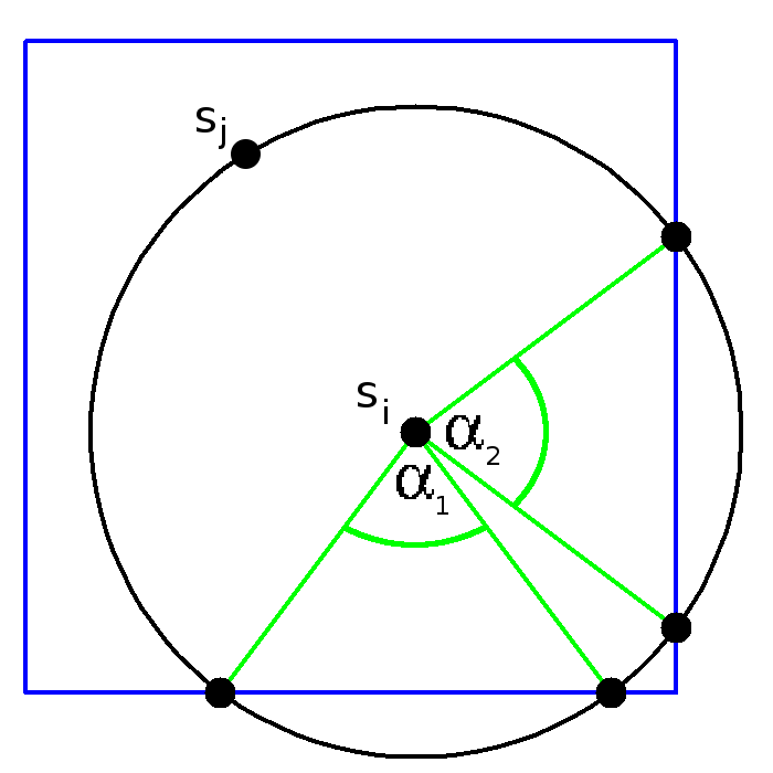
Practical aspects of implementation. We propose to use a non-parametric kernel estimator as discussed by Stoyan and Stoyan (1992) (Part III, Chapter 5.4.2). Consider , then we estimate the pair correlation function by
with the Epanechnikov kernel , and kernel weights for edge correction (see Ripley (1977)). These are defined as which is the ratio of the whole circumference of to the circumference within , i.e is the sum of all angles, for which the associated non-overlapping circle arcs are within , see Figure 8.
Remark 19.
The estimates of and obtained from by the minimum contrast method, have a very high variance. Therefore, this procedure is only recommended if we observe several i.i.d. realizations of and the associated . The final estimates of and may then be defined as the mean or median of the estimates obtained from .


Plots of the estimated pair correlation functions via a sample of and by points of are compared in Figure 9. They are also compared to the true pair correlation function and the natural benchmark which is obtained from a direct sample of instead of . Numerical experiments such as reported in Figure 9 and Section 6 support that our proposed modification works surprisingly well.
6 Simulation study
We survey the performance of our proposed non-parametric estimator (4.8) of the realization of and that of the estimators and (5.3) of the parameters of the covariance function of in a simulation study.
Setting. In our numerical experiments we choose the covariance of the underlying Gaussian process to be the Whittle-Matérn model (2.11) with known smoothness parameter and unknown variance and scale . The scale will control the size of clusters in our point processes and the variance directs the variability of the number of points within the local clusters. The performances of the associated estimators are compared for different choices and . As shape mechanism we consider the fixed storm process where is the density of the standard normal distribution. We simulate realizations of the corresponding Cox extremal process on an equidistant grid with grid points in .
Henceforth, we simplify the notation from the previous section by writing instead of for the estimated intensity function. A natural benchmark of our estimation procedures from Sections 4 and 5 are such estimators which are derived from direct samples of a Cox process with spatial intensity process . We denote the benchmark kernel estimator by
| (6.1) |
Accordingly, let and be the minimum contrast estimators obtained from direct samples of .
Measures for evaluation. To assess the performance of our non-parametric estimates we use the following mean relative variance
| (6.2) |
with for .
Up to a scaling constant, is an empirical version of with
We compare the of our estimated intensity with that of the benchmark . The corresponding relative of and is defined as the ratio .
The goodness of fit of the parametric estimates is measured in terms of the empirical mean squared error
.
Again the of and are compared with those of the benchmark estimators and , respectively.
Results. The results of our simulation study are reported in the tables of Figures 10 and 11 in Appendix A.1. The best performance we can hope for is to be as good as the benchmark estimators that are applied to samples of the original point process . Hence, in the case of our non-parametric estimation of the realisations of the intensity processes we can expect the ratios to be always greater or equal to and at best even close to . Indeed, this is confirmed by the simulation study as can be seen from Figure 10. All ratios (except one) lie slightly above 1. The exceptional case occurs when the standard error of is relatively high, where we even outperform the benchmark. This is quite remarkable given that we infer the intensity under an independence assumption that is not necessarily satisfied (cf. Section 7 for a discussion) and secondly, we correct it by a data driven quotient as in (4.3).
Likewise we observe that the standard errors for the MRV are close to the benchmark when and much smaller – sometimes even half the size – in the case . This indicates that our estimation procedure for is relatively stable compared to the benchmark. In general, both estimators perform better for the larger value of the scale parameter , that is for larger cluster sizes in the point processes, whereas a higher variance naturally leads to a worse performance. The influence of the smoothness parameter is not entirely clear. Looking at the values one might conclude that the estimation improves for a smoother intensity. But in case of the smoothest field () the MRVs get larger again. However, what is more important is that both procedures, the one that we proposed for inference on for Cox extremal processes and the benchmark , behave coherently as the parameters vary across different smoothness classes, cluster sizes and variability of number of points within local clusters.
The non-parametric estimates are further used to obtain the parametric estimates of and . Here, estimation of the pair correlation function is very sensitive to the choice of the scale. Our maximal scale is large in relation to the size of the observation window which causes a bias in the estimation of all pair correlation functions. Therefore, all parametric estimates – the benchmarks as well as our estimates – are also biased when . The estimation of is volatile if , this applies in particular to our which fails when both and . Still, in all other cases the of our multi-stage estimators is close to that of the benchmark. There are even some cases when we outperform the benchmark, which is not surprising as the standard errors are very high in general.
7 Discussion
In this article we present a new class of conditionally max-stable random fields based on Cox processes, which we therefore also call Cox extremal processes. We prove in Theorem 7 that these processes are in the MDA of familiar max-stable models. Hence, they have the potential to model spatial extremes on a smaller time scale.
An objective of practical importance is to identify the random effects influencing the underlying Cox process from the centres of the contributing storms. In order to make inference feasible, we impose an additional independence assumption on our observed data (see Lemma 10) that allows to derive a uniformly consistent non-parametric kernel estimator (4.5) for the realization of the intensity process (Corollary 12). Imposing such an independence assumption can be seen in a similar manner to the composite likelihood method that ignores dependence among higher order tupels. We believe that our condition is sufficiently well satisfied in most situations, since only a small number of large storms from the Cox process approximate the Cox extremal process already quite well. Practical adjustments of the estimator (4.5), in particular to a non-asymptotic setting, are presented in Section 4.2.
For parametric estimation the non-parametric estimator (4.8) can be used to correct the observed point processes of contributing storm centres in order to obtain samples from (Lemma 15). If is log Gaussian, the minimum contrast method can be applied subsequently to obtain estimates for the parameters of the covariance function of .
The performance of our proposed estimation procedures is addressed in a simulation study (Section 6). Here, the best we can hope for is that our estimators can compete with the benchmark estimators applied to the original point process . Indeed, our non-parametric procedure is usually relatively close to the benchmark which is quite remarkable in view of the necessary adjustments we have to make. Also, looking at different kinds of smoothness, cluster sizes and variances we find evidence for the stability of our proposed estimation procedure when compared to the benchmark. Both (our procedure and the benchmark) behave coherently across different choices of these properties. Similar behaviour can be observed for the parametric estimates, even though they are more volatile and the estimation of the pair correlation function is generally very sensitive to the choice of scale.
Within our simulation study and all other illustrations, we consider deterministic storm processes where is the density of the standard normal distribution. This restriction is only done to reduce the computing time. Indeed, all estimators presented in Section 4 and 5 are valid for much more general and simulations showed that the specification of only slightly influences the inference on as long as enough centres of contributing storms can be identified. For instance, if we impose the monotonicity assumption (2.12) on the storm process , the majority can be recovered as local maxima of the realization of . Computational methods for identification of such points are left for further research.
Acknowledgments. The research of MD was partly supported by the DFG through ’RTG 1953 - Statistical Modeling of Complex Systems and Processes’ and Volkswagen Stiftung within the project ’Mesoscale Weather Extremes - Theory, Spatial Modeling and Prediction’. The authors are grateful to A. Baddeley for useful comments on the estimation of pair correlation functions and thank M. Oesting for a discussion of simulation algorithms for max-stable processes.
Appendix A Appendix
A.1 Simulation results


A.2 Preliminaries on point processes
In this article, we follow the conventions based on Daley and Vere-Jones (2003); Daley and Vere-Jones (2008) briefly reviewed here. Let be a complete separable metric space, and its Borel -field. A Borel measure on is called boundedly finite if for locally compact Borel sets . The space of all boundedly finite measures on is denoted by and its subspace of simple counting measures by . Both spaces, and , are itself complete separable metric spaces if endowed with the weak hash topology, see Appendix 2.6 in (Daley and Vere-Jones, 2003). Let and be the smallest -algebra on and accordingly , for which the mappings respectively are measurable for all in . A random measure is a measurable mapping from a probability space to and accordingly a point process is a measurable mapping from to . Note that a point process, as defined here, always allows for a measurable enumeration, see Lemma 9.1.XIII in Daley and Vere-Jones (2008). Convergence of random measures and point processes is always meant in the sense of weak convergence in and , respectively.
A.3 Proofs
A.3.1 Proofs for Section 2
Lemma 1.
The point process on the left-hand side equals in distribution the -thinning of with . Hence, by Theorem 11.3.III in Daley and Vere-Jones (2008) the desired convergence holds true if and only if converges to , which follows from the multivariate law of large numbers and Theorem 11.1.VII in Daley and Vere-Jones (2008). ∎
Lemma 2.
We follow closely the arguments of (Kabluchko et al., 2009, Proposition 13). For and , set
- (a)
Conditional on the the process , the number of points in is Poisson distributed with parameter
which is -almost surely finite by the integrability condition (2.4). Hence, the number of points in is almost surely finite, which entails that
is almost surely finite.
- (b)
Under the additional condition (2.5), there exists , such that
almost surely. That is, the process can be represented on as the maximum of a finite number of continuous functions, which ensures the continuity of on .
∎
Lemma 4.
Due to its compactness, can be split into finitely many (possibly overlapping) compact pieces of diameter less than . Since almost surely, there are almost surely infinitely many elements in of the Cox process (that underlies the construction of ) in each of these pieces , . Since there exists an such that , there exists almost surely an element (in fact, infinitely many elements) within the Cox process, such that . Summarizing, is almost surely covered by
Setting and , we deduce that
is strictly greater than zero as desired. ∎
Remark 20.
In fact, the condition in Lemma 4 may be further relaxed to the requirement
Lemma 6.
Due to the stationarity of and the invariance of the Lebesgue measure with respect to translations, we obtain
∎
We will now prove Theorem 7, the main result of Section 2, i.e. the weak convergence of the random fields
To this end we set the left-hand-side which can be more conveniently represented as
where is a Cox-process on , directed by the random measure
and , represent i.i.d. copies of . The random measure is the directing measure of the union of the underlying independent Cox-processes of the random fields , , scaled by . By Lemma 1, the point process converges weakly to the Poisson-process with directing measure
that underlies the mixed moving maxima random field . The latter convergence indicates already the result of Theorem 7. In order to prove Theorem 7, we show first the convergence of the finite dimensional distributions and then the tightness of the sequence , .
Lemma 21 (Convergence of finite-dimensional distributions).
Let the random fields and be specified as in Theorem 7, then the finite dimensional distributions of converge to those of as .
Proof.
We fix and show that the random vector lies in the max-domain of attraction of the random vector . It then automatically follows that the finite dimensional distributions converge to those of , since the scaling constants for each individual are chosen appropriately.
For , it follows from (2.8) that the non-negative random variable
satisfies that its first moment is finite and can be gained from its Laplace transform via
Hence, by l’Hôpital’s rule
with . Moreover, is a multiple of the exponent function of the max-stable random vector
Hence, by (Resnick, 2008, Corollary 5.18 (a)), the random vector lies in its domain of attraction. ∎
The following lemma will be useful to prove the tightness of the sequence .
Lemma 22.
Let and be bounded sequences of non-negative real numbers, then
Proof.
The statement is the triangle inequality with the norm in the space of bounded sequences. ∎
Lemma 23 (Tightness).
Let the random field be specified as in Theorem 7, then the sequence of random fields is tight.
Proof.
Since the finiteness of does also ensure the finiteness of each , it suffices to show that, for a compact set , the modulus of continuity
satisfies the convergence
| (A.1) |
To simplify the notation, we introduce . By the definition of and the preceding Lemma 22, we have
As the tuples , are the points of the Cox process , we can compute the latter probability as expected void-probability. To this end, let us denote the joint probability law of the i.i.d. intensity processes , and its expectation by and , respectively. Setting , we obtain
where the last inequality follows from Fatou’s Lemma. Moreover, the strong law of large numbers and condition (2.4) (which ensures the existence and finiteness of the following right-hand side) yield that -almost surely
which entails
Finally, in order to establish (A.1), it remains to be shown that
This, however, follows from the dominated convergence theorem, since for any fixed
and any fixed the convergence of the integrand to holds true and by
and condition (2.7), there exists an integrable upper bound. ∎
We are now in position to prove the main result of Section 2.
Theorem 7.
The finiteness and sample-continuity of the random fields and are an immediate consequence of Lemma 2. While Lemma 21 shows that the finite-dimensional distributions of the random fields converge to those of the process , Lemma 23 establishes the tightness of the sequence . Collectively, this proves the assertions. ∎
A.3.2 Proofs for Section 3
Proposition 8.
First note that is a Poisson process on with intensity 1. Hence is a Poisson process on with intensity . Attaching the independent markings and, for fixed , the markings yields that, for fixed , the point process is a Poisson process directed by the measure on .
Since in the construction of only storms with center in can contribute to the process on , the law of on and the law of
coincide. By definition of the stopping time and since is uniformly bounded by , the latter has the same law as the process on . So, it remains to be shown that is almost surely finite.
Similar to the proof of Lemma 4, it can be shown that
| (A.2) |
Together with the decrease of the sequence this implies the a.s.-finiteness of . ∎
A.3.3 Proofs for Section 4
Lemma 10.
Since is independent of , the process is an independent thinning of the Poisson process . The number of points in the set
is Poisson distributed with parameter
This finishes the proof. ∎
Theorem 11.
The paths of the intensity process are almost surely continuous and is even uniformly continuous since its support equals the compact set . Therefore, the integral is finite. Hence all assumptions of Theorem 3.1.7. in Prakasa Rao (1983) hold true, which proofs the statement. ∎
Corollary 12.
Lemma 13.
The assertion follows from the straight forward computation
Since the number of points in is Poisson distributed with parameter
we conclude
∎
References
- Adler (1981) R. J. Adler. The geometry of Random fields. John Wiley & SonsLtd, 1981.
- Blanchet and Davison (2011) J. Blanchet and A. C. Davison. Spatial modeling of extreme snow depth. Ann. Appl. Stat., 5(3):1699–1725, 2011.
- Castruccio et al. (2015) Stefano Castruccio, Raphael Huser, and Marc G. Genton. High-order composite likelihood inference for max-stable distributions and processes. J. Comput. Graph. Statist., 2015.
- Cooley (2005) D. Cooley. Statistical Analysis of Extremes Motivated by Weather and Climate Studies: Applied and Theoretical Advances. PhD thesis, University of Colorado, 2005.
- Cox (1955) D. R. Cox. Some statistical models connected with series of events. J. R. Stat. Soc. Ser. B Stat. Methodol., 17:129–164, 1955.
- Daley and Vere-Jones (2003) D. J. Daley and D. Vere-Jones. An Introduction to the Theory of Point Processes: Volume I: Elementary Theory and Methods. Springer, 2003.
- Daley and Vere-Jones (2008) D. J. Daley and D. Vere-Jones. An Introduction to the Theory of Point Processes: Volume II: General Theory and Structure. Springer, 2008.
- de Haan (1984) L. de Haan. A spectral representation for max-stable processes. Ann. Probab., 12(4):1194–1204, 1984.
- de Haan and Ferreira (2006) L. de Haan and A. Ferreira. Extreme value theory. Springer Series in Operations Research and Financial Engineering. Springer, New York, 2006. An introduction.
- Dieker and Mikosch (2015) A. B. Dieker and T. Mikosch. Exact simulation of Brown-Resnick random fields at a finite number of locations. Extremes, 18(2):301–314, 2015.
- Diggle (1985) P. J. Diggle. A kernel method for smoothing point process data. J. Roy. Statist. Soc. Ser. C, 34:138–147, 1985.
- Diggle and Gratton (1984) P. J. Diggle and R. J. Gratton. Monte carlo methods of inference for implicit statistical models. J. R. Stat. Soc. Ser. B Stat. Methodol, 46(2):193–227, 1984.
- Diggle et al. (2013) P. J. Diggle, P. Moraga, B. Rowlingson, and B. M. Taylor. Spatial and spatio-temporal log-Gaussian Cox processes: extending the geostatistical paradigm. Statist. Sci., 28(4):542–563, 2013.
- Dombry (2012) C. Dombry. Extremal shot noises, heavy tails and max-stable random fields. Extremes, 15(2):129–158, 2012.
- Dombry and Eyi-Minko (2013) C. Dombry and F. Eyi-Minko. Regular conditional distributions of continuous max-infinitely divisible random fields. Electron. J. Probab, 18:no. 7, 21, 2013.
- Dombry et al. (2016) C. Dombry, S. Engelke, and M. Oesting. Exact simulation of max-stable processes. Biometrika, 2016.
- Engelke et al. (2011) S. Engelke, Z. Kabluchko, and M. Schlather. An equivalent representation of the Brown-Resnick process. Statist. Probab. Lett., 81(8):1150–1154, 2011.
- Engelke et al. (2015) S. Engelke, A. Malinowski, Z. Kabluchko, and M. Schlather. Estimation of Hüsler-Reiss distributions and Brown-Resnick processes. J. R. Stat. Soc. Ser. B Stat. Methodol, 77(1):239–265, 2015.
- Genton et al. (2015) M. G. Genton, S. A. Padoan, and H. Sang. Multivariate max-stable spatial processes. Biometrika, 102(1):215–230, 2015.
- Giné et al. (1990) E. Giné, M. G. Hahn, and P. Vatan. Max-infinitely divisible and max-stable sample continuous processes. Probab. Theory Related Fields, 87(2):139–165, 1990.
- Guttorp and Gneiting (2006) P. Guttorp and T. Gneiting. Studies in the history of probability and statistics. XLIX. On the Matérn correlation family. Biometrika, 93(4):989–995, 2006.
- Heinrich and Molchanov (1994) L. Heinrich and I. S. Molchanov. Some limit theorems for extremal and union shot-noise processes. Math. Nachr., 168:139–159, 1994.
- Jourlin et al. (1988) M. Jourlin, B. Laget, G. Matheron, F. Meyer, F. Preteux, M. Schmitt, and J. Serra. Image Analysis and Mathematical Morphology. Volume 2: Theoretical Advances. Academic Press, Inc., London, 1988.
- Kabluchko et al. (2009) Z. Kabluchko, M. Schlather, and L. de Haan. Stationary max-stable fields associated to negative definite functions. Ann. Probab., 37(5):2042–2065, 2009.
- Liu et al. (2016) Z Liu, J Blanchet, A.B. Dieker, and T. Mikosch. Optimal exact simulation of max-stable and related random fields. arXiv:1609.06001, 2016.
- Matheron (1987) G. Matheron. Suffit-il, pour une covariance, d’etre de type positif? Sciences de la terre, serie informatique geologique, 26, 1987.
- Møller and Schoenberg (2010) J. Møller and F. P. Schoenberg. Thinning spatial point processes into poisson process. Adv. in Appl. Probab., 42(2):347–358, 2010.
- Møller and Waagepetersen (2004) J. Møller and R. P. Waagepetersen. Statistical inference and simulation for spatial point processes, volume 100 of Monographs on Statistics and Applied Probability. Chapman & Hall/CRC, Boca Raton, FL, 2004.
- Møller et al. (1998) J. Møller, A. R. Syversveen, and R. P. Waagepetersen. Log Gaussian Cox Processes. Scand. J. Statist., 25:451–482, 1998.
- Nadarajah et al. (1998) S. Nadarajah, C.W. Anderson, and J. A. Tawn. Ordered multivariate extremes. J. R. Stat. Soc. Ser. B Stat. Methodol., 60:473–496, 1998.
- Nolan (2016) J. Nolan. Stable Distributions : Models for Heavy-Tailed Data. Birkhauser, 2016.
- Oesting and Schlather (2014) M. Oesting and M. Schlather. Conditional sampling for max-stable processes with a mixed moving maxima representation. Extremes, 17(1):157–192, 2014.
- Oesting et al. (2012) M. Oesting, Z. Kabluchko, and M. Schlather. Simulation of Brown-Resnick processes. Extremes, 15(1):89–107, 2012.
- Oesting et al. (2013) M. Oesting, M. Schlather, and C. Zhou. On the normalized spectral representation of max-stable processes on a compact set. arXiv:1310.1813v1, 2013.
- Oesting et al. (2015) M. Oesting, M. Schlather, and P. Friederichs. Statistical post-processing of forecasts for extremes using bivariate brown-resnick processes with an application to wind gusts. arXiv:1312.4584v2, 2015.
- Opitz (2013) T. Opitz. Extremal processes: elliptical domain of attraction and a spectral representation. J. Multivariate Anal., 122:409–413, 2013.
- Prakasa Rao (1983) B. L. S. Prakasa Rao. Nonparametric functional estimation. Probability and Mathematical Statistics. Academic Press, Inc., New York, 1983.
- Resnick (2008) S. I. Resnick. Extreme values, regular variation and point processes. Springer Series in Operations Research and Financial Engineering. Springer, New York, 2008. Reprint of the 1987 original.
- Ripley (1977) B. D. Ripley. Modelling spatial patterns. J. R. Stat. Soc. Ser. B Stat. Methodol., 39(2):172–212, 1977. With discussion.
- Samorodnitsky and Taqqu (1994) G. Samorodnitsky and M. S. Taqqu. Stable non-Gaussian random processes. Stochastic Modeling. Chapman & Hall, New York, 1994. Stochastic models with infinite variance.
- Schlather (2002) M. Schlather. Models for stationary max-stable random fields. Extremes, pages 33–44, 2002.
- Schlather and Tawn (2003) M. Schlather and J. A. Tawn. A dependence measure for multivariate and spatial extreme values: Properties and inference. Biometrika, 90(1):139–156, 2003.
- Serra (1984) J. Serra. Image analysis and mathematical morphology. Academic Press, Inc., London, 1984. English version revised by Noel Cressie.
- Smith (1990) R. L. Smith. Max-stable processes and spatial extremes. Unpublished Manuscript, 1990.
- Stephenson et al. (2015) A. G. Stephenson, B. A. Shaby, B. J. Reich, and A. L. Sullivan. Estimating spatially varying severity thresholds of a forest fire danger rating system using max-stable extreme-event modeling. J. Appl. Meteor., 54(2), 2015.
- Stoev (2008) S. A. Stoev. On the ergodicity and mixing of max-stable processes. Stochastic Process. Appl., 118(9):1679–1705, 2008.
- Stoev and Taqqu (2005) S. A. Stoev and M. S. Taqqu. Extremal stochastic integrals: a parallel between max-stable processes and -stable processes. Extremes, 8(4):237–266 (2006), 2005.
- Stoev and Taqqu (2006) S. A. Stoev and M. S. Taqqu. How rich is the class of multifractional Brownian motions? Stochastic Process. Appl., 116(2):200–221, 2006.
- Stoyan and Stoyan (1992) D. Stoyan and H. Stoyan. Fraktale - Formen - Punktbilder. 1992.
- Zhang and Smith (2004) Z. Zhang and R. L. Smith. The behavior of multivariate maxima of moving maxima processes. J. Appl. Probab., 41(4):1113–1123, 2004.