Interactive Preference Learning of
Utility Functions for Multi-Objective Optimization
Abstract
Real-world engineering systems are typically compared and contrasted using multiple metrics. For practical machine learning systems, performance tuning is often more nuanced than minimizing a single expected loss objective, and it may be more realistically discussed as a multi-objective optimization problem. We propose a novel generative model for scalar-valued utility functions to capture human preferences in a multi-objective optimization setting. We also outline an interactive active learning system that sequentially refines the understanding of stakeholders ideal utility functions using binary preference queries.
1 Introduction
As machine learning systems become more prominent across industries and organizations, it is important that they be tuned so as to perform as optimally as possible. One method that has been increasingly popular in identifying the configuration of an optimal machine learning system is Bayesian black-box optimization of the hyperparameter configurations of machine learning models [14] [16] [6]. However, most of these techniques require that the objective be a scalar valued function depending on the hyperparamter configuration ; in the context of machine learning, this objective is often a scalar-valued cross-validated metric . The space of hyperparameter configurations is left intentionally ambiguous.
In practice however, the performance of real systems is often more naturally discussed using a vector of competing metrics
where is the space of possible metric values (in this article, we assume ). This allows for the perspectives of various stakeholders regarding the aspects of an optimal system to be captured.
For general machine learning systems, this competition may involve trade-offs between predictive accuracy and computational cost of a model [8] [12]. The trade-off between precision and recall can be phrased in this format, and indeed, all classification problems with unbalanced class representation, such as fraud or spam tasks, might be best addressed using a different metric associated with the loss estimate for each class [7].
Indeed, it is standard that engineering systems are designed based on varied input from the involved stakeholders; this naturally leads to a discussion of several metrics related to the performance of the system. We might pose such a problem, involving the accumulation of competing metrics and finding an optimal configuration, as
Here, denotes a utility function which, in a likely implicit fashion, encapsulates a balance in the preferences between stakeholders.
Of course, the implicit nature of this utility function is a significant stumbling block in any optimization process: it may be simple for developers of a loan prediction model to specify a need to balance the expected false repayment and false default predictions, but optimally defining their interaction in the business context is more complicated. This article proposes a model for this utility function in Section 2 based on the idea that the function is formed by a product of “individual utilities” over individual metrics. We explore the impact of free parameters in the structure of and then, in Section 3 explain how these free parameters can be appropriately selected through a thought experiment that stakeholders supervising the machine learning system conduct before attempting to find . This concept of interactively conducting a multiobjective optimization was discussed in [1]. Section 5 presents some manufactured experiments which demonstrate the viability of this interactive questioning mechanism to accurately reproduce the behavior of a predefined, but unknown, utility function.
2 Generative Model for Multi-objective Utility Functions
We propose a utility function composed of a product of one dimensional individual 11 1 The ideal term here would be marginal utility functions (analogous to marginal densities) but the term marginal utility has a specific meaning in the context of economics so we prefer the term individual utility instead. utility functions
Each of these individual utility functions could take arbitrary structure; we choose to impose the form of cumulative distribution functions of beta random variables, so that
where is the beta function and and represent two free parameters governing the shape of the beta density. We enforce the belief that these parameters are log-normal with unknown variance,
| (1) |
and describe in Section 2.1 how these and parameters are chosen. We also, at times, use a slight abuse of notation, , to suppress the presence of the parameters in the utility. This structure (the product of distribution functions) has appeared in other literature, although in the context of adapting non-stationary data for use in stationary Gaussian processes [15].
Some of the existing literature on designing a utility function involves the use of an additive, rather than multiplicative, combination of marginal utilities [1]. We believe that the multiplicative structure is potentially more suitable for utility functions with a nonlinear structure, such as those presented in Section 5 involving constraints or the -score style utilities designed to balance precision and recall.
For all , the resulting utility function will monotonically increase on the domain . This is a byproduct of the fact that each individual utility is monotonically increasing which enforces the standard assumption for multicriteria problems that in an ideal setting all metrics should be optimized and thus any increase in one with no decrease in others is an improvement in utility. Specifically, for a particular and , the following will hold,
2.1 Marginal Likelihood for Binary Preference Data
The motivation behind the development of this utility model is the need to balance the input from multiple, possibly competing, stakeholders during the production of a machine learning system with multiple competing metrics which define success. As such, it may be difficult or controversial to judge the value of a specific set of metrics in absolute terms (i.e., for an engineer or product manager to assign a scalar value associated with the quality of ).
In contrast, it is generally considered a simpler task to compare two sets of metric values and state which of the two is “better” [4]. To reduce cognitive load on our eventual users, we consider exactly this approach, where the only information that stakeholders must provide is a stated preference between proposed vectors of metric values and .
Our mechanism, described in Section 3, solicits this binary preference between the (implicit) utilities of two multi-objective value configurations with the hope of learning an appropriate model of the form described in Section 2. Stakeholders may also lack a significant utility preference between two possible configurations, and our model accounts for this perceptual uncertainty by allowing users to report that two configurations are perceived to have equal22 2 In this setting, we allow for users to specify that objective vectors and have equal utility either because they are perceived to perform equally well or equally poorly. utility. Thus, we allow for two types of observations from users: pairs of multi-objective values where a clear preference in utility is observed (denoted by ) and pairs of configurations where no preference is specified (denoted by ),
We quantify this lack of preference by imposing an insensitivity to utilities which differ by too small a margin; this margin is defined probabilistically by an equivalence distance , where is an additional hyperparameter.
We now define a parametrization strategy based on marginal likelihood to help find the best hyperparameters
given specific results and . We design this parametrization metric to produce utility functions that better adhere to observed preferences (because they should be seen as more likely). We define an auxiliary function
which describes the distance from utilities for given parameters. The likelihood function, then, is defined differently for the sets with and without stated preferences:
where is the Heaviside function. The quantity associated with mimics the computation of the p-value in a 2-tailed statistical test. No simple analytic form is known for this likelihood (so far) so we estimate it using Monte Carlo techniques.
3 Active Preference Learning of Utility Functions
Given the likelihood defined in Section 2.1, it is feasible to take a large set of (and possibly ) results and optimally fit the model parameters with, e.g., sequential model-based optimization (SMBO) [2, 9, 13]. This strategy optimizes an expensive, and possibly black-box, objective function by suggesting inputs to be evaluated and incorporating the resulting observed objective values into an appropriate surrogate model of the objective. The updated surrogate model is then used to optimally make the next suggestion by identifying points believed to most benefit the optimization search.
However, before this model fitting can take place, it is necessary to generate the and data. This process involves soliciting preferences from stakeholders, which is considered an expensive process (likely much more expensive than the likelihood evaluation, even with the Monte Carlo estimation). As such, we propose the use of SMBO to identify the best questions to ask so as to minimize the demands on the stakeholders. The approach has previously proved useful for conducting interactive optimizations with a human in the loop where the implicit objective is related to that user’s perception. In particular, Brochu [3] [5] demonstrated the viability of the idea for interactively learning optimal parameter configurations in computer graphics settings.
In this setting, we no longer seek the optimum of some latent objective; indeed for every possible utility function, that optimal configuration is always known (simply maximizing each individual metric value). The aim, instead, is to select preference queries that would help to resolve uncertainty about the user’s latent utility function. This process is outlined below in Algorithm 1. Initial preference data is collected from the user using no information about the utility model. Each subsequent preference query begins with fitting the utility model to all the preference data observed so far. An acquisition function (discussed in Section 3.1) that ranks pairs of configurations is then maximized to determine which two configurations to present to the user. The datasets are updated with the preference information and the process continues.
3.1 Single and Pairwise Maximum Entropy Search
As described in the previous section, we need an acquisition function with which to propel the SMBO. The goal of that acquisition function is to design questions that will reduce our uncertainty in the MLE of the utility function model. Entropy based search policies have been used in the literature for selecting instances for labeling in active learning settings for machine learning models [11]. In our context, the task is to decide which pair of configurations would give us the most information about our utility function model.
We define an entropy-like condition to power the search for the two metric configurations whose difference in utility has the greatest uncertainty. Under a Gaussian assumption, the entropy of a random variable is a monotonic function of its variance [11], so we can use the empirical variance of samples of the utility differences to approximate the entropy,
where follow the distribution defined in (1) with hyperparameters from . This formulation, labeled “pairwise entropy”, assumes we are searching for two new configurations for the user to compare each iteration. An alternative strategy is to keep the preferred configuration and fix to take that value in the next search, varying only . This search strategy is labeled “single entropy”. The distinction is pertinent in Section 5.
It is important to note that we enforce that the configuration pairs presented to users always exhibit the property , so that we are not merely asking users to compare configurations with an already assumed preference based on our utility being monotonic.
4 Interactive Tool for Utility Preference Queries
To realize the full benefit of incorporating many perspectives on the optimality of a system, we outline a simple interface for our utility preference solicitation system that is easy to understand even for groups of users having a broad range of technical sophistication.
4.1 Multi-objective Utility Comparison Cards
To visualize two multi-objective value configurations, our system uses a simple back-to-back bar chart as shown in Figure 1. Users are asked to select which configuration they perceive as having higher utility. It is worth noting that alternate visualizations could be used in place of the one outlined here, including ones that do not directly expose the numeric value of the underlying metrics but rely on more system-specific visual summaries.

4.2 Visualization of Utility Functions
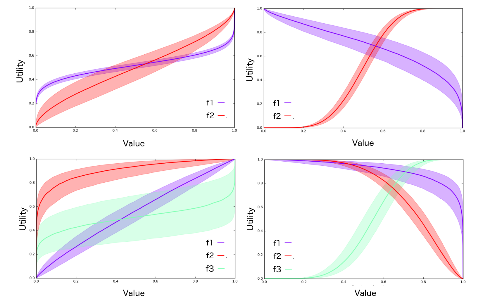
Since the learned utility is a product of cumulative distribution functions, these distributions can be independently visualized to give the user an intuition about the components of the full product utility function. The MLE of the hyperparameters governing the distribution of the terms can serve users as a direct introspection mechanism into the uncertainty associated with the learned individual utilities. Figure 2 shows an example of these independent utility plots for several test utility functions with their mean and interquartile range highlighted; Figure 3 shows the actual utility learned from three sample implicit utilities.
3. max 4. min
Figure 2 provides some confidence in the learned joint utility functions. For example, consider the top right plot (2), corresponding to the test utility : min . We can see that the model has attempted to learn the threshold constraint of . We see that the individual utility for has a sharp, non-linear spike around 0.6. In the full utility function product then, configurations with will be zeroed out and those with , the utility function will take on the values of . We can also see that the individual utility plot of is a mostly linear looking monotonically decreasing function, maximized when and minimized when which corresponds nicely to a utility function for a metric we aim to minimize. We allow in the specification of the model for metrics to defined as optimally minimized or maximized. The individual utility for minimization metrics is defined as the survival function of the beta cumulative distribution.

5 Experimental Results
A series of experiments were conducted to evaluate the performance of the learned utility function model using several active search policy variations. Explicit test utility functions were used to simulate implicit human utility functions. We include two test utilities that correspond to the and scores commonly used in machine learning and information retrieval [10]. We also include test utility functions that incorporate threshold constraints. These threshold constrained tests were simulated in the following way: if both configurations violated the constraints, the configurations were reported with equal perceived utility.
A hold-out set of 10,000 random multi-objective configurations were generated for each test function and the Kendall rank correlation coefficient was used to quantify the ordinal association between the test utility function values and the learned utility function values for all 10,000 configurations. Since the region of the feasible solutions is not known a priori, our learned utility must strive to ensure that the utility is consistent over the entire domain.
Each method was allowed binary preference queries where is the number of metrics. The active search strategies were initialized with randomly selected configurations. We report the average Kendall correlation score after 5 runs using each search algorithm on the same generated hold-out set.
| Test Utility Function | Rnd Search | Single Entropy | Pair Entropy |
|---|---|---|---|
| max | 0.8756 | 0.8542 | 0.8618 |
| max | 0.9422 | 0.9448 | 0.9615 |
| min | 0.6507 | 0.6805 | 0.6893 |
| max | 0.8844 | 0.9028 | 0.9039 |
| max | 0.8949 | 0.8950 | 0.9120 |
| max | 0.8490 | 0.8018 | 0.7805 |
| max | 0.8738 | 0.8516 | 0.8311 |
| min s.t. | 0.2949 | 0.3154 | 0.3257 |
| max | 0.2309 | 0.2088 | 0.2648 |
From these results, our proposed utility model appears to perform well under the various acquisition functions. The performance of the random search policy is particularly noteworthy as it avoids fitting the utility model each iteration and therefore much less expensive computationally. The mean performance of the pair entropy search seems to edge out the other methods on most of the examples with the interesting exception of the linear test utility functions.
Future work could involve experiments using real human users on a relevant machine learning system building task. In addition, further investigations into the utility function model and acquisition function could prove valuable in capturing certain utilities.
References
- [1] Valerie Belton, Jürgen Branke, Petri Eskelinen, Salvatore Greco, Julian Molina, Francisco Ruiz, and Roman Slowiński. Multiobjective optimization. chapter Interactive Multiobjective Optimization from a Learning Perspective, pages 405–433. Springer-Verlag, Berlin, Heidelberg, 2008.
- [2] James S Bergstra, Rémi Bardenet, Yoshua Bengio, and Balázs Kégl. Algorithms for hyper-parameter optimization. In Advances in Neural Information Processing Systems, pages 2546–2554.
- [3] Eric Brochu, Tyson Brochu, and Nando de Freitas. A bayesian interactive optimization approach to procedural animation design. In Proceedings of the 2010 ACM SIGGRAPH/Eurographics Symposium on Computer Animation, pages 103–112. Eurographics Association, 2010.
- [4] Wei Chu and Zoubin Ghahramani. Preference learning with gaussian processes. In Proceedings of the 22nd international conference on Machine learning, pages 137–144. ACM, 2005.
- [5] Brochu Eric, Nando D Freitas, and Abhijeet Ghosh. Active preference learning with discrete choice data. In Advances in neural information processing systems, pages 409–416, 2008.
- [6] M. Feurer, A. Klein, K. Eggensperger, J. Springenberg, M. Blum, and F. Hutter. Efficient and robust automated machine leraning. In Advances in Neural Information Processing Systems 28, pages 2944–2952, December 2015.
- [7] Jonathan E Fieldsend. Optimizing decision trees using multi-objective particle swarm optimization. In Swarm intelligence for multi-objective problems in data mining, pages 93–114. Springer, 2009.
- [8] Daniel Hernández-Lobato, José Miguel Hernández-Lobato, Amar Shah, and Ryan P Adams. Predictive entropy search for multi-objective bayesian optimization. arXiv preprint arXiv:1511.05467, 2015.
- [9] Frank Hutter, Holger H Hoos, and Kevin Leyton-Brown. Sequential model-based optimization for general algorithm configuration. In Learning and Intelligent Optimization, pages 507–523. Springer, 2011.
- [10] C. J. Van Rijsbergen. Information Retrieval. Butterworth-Heinemann, Newton, MA, USA, 2nd edition, 1979.
- [11] Burr Settles. Active learning literature survey. University of Wisconsin, Madison, 52(55-66):11, 2010.
- [12] Amar Shah and Zoubin Ghahramani. Pareto frontier learning with expensive correlated objectives. In Proceedings of The 33rd International Conference on Machine Learning, pages 1919–1927, 2016.
- [13] Bobak Shahriari, Kevin Swersky, Ziyu Wang, Ryan P. Adams, and Nando de Freitas. Taking the human out of the loop: A review of bayesian optimization. Technical report, Universities of Harvard, Oxford, Toronto, and Google DeepMind, 2015.
- [14] Jasper Snoek, Hugo Larochelle, and Ryan P Adams. Practical bayesian optimization of machine learning algorithms. In Advances in neural information processing systems, pages 2951–2959, 2012.
- [15] Jasper Snoek, Kevin Swersky, Richard S Zemel, and Ryan P Adams. Input warping for bayesian optimization of non-stationary functions. In ICML, pages 1674–1682, 2014.
- [16] C. Thornton, F. Hutter, H. H. Hoos, and K. Leyton-Brown. Auto-WEKA: Combined selection and hyperparameter optimization of classification algorithms. In Proceedings of the 19th ACM SIGKDD international conference on Knowledge discovery and data mining, pages 847–855. ACM, 2013.