Projected distances to host galaxy reduce SNIa dispersion
Abstract
We use multi-band imagery data from the Sloan Digital Sky Survey (SDSS) to measure projected distances of 302 supernova type Ia (SNIa) from the centre of their host galaxies, normalized to the galaxy’s brightness scale length, with a Bayesian approach. We test the hypothesis that SNIae further away from the centre of their host galaxy are less subject to dust contamination (as the dust column density in their environment is smaller) and/or come from a more homogeneous environment. Using the Mann-Whitney U test, we find a statistically significant difference in the observed colour correction distribution between SNIae that are near and those that are far from the centre of their host. The local -value is , which is significant at the 5 per cent level after look-elsewhere effect correction. We estimate the residual scatter of the two subgroups to be for the far SNIae, compared to for the near SNIae – an improvement of 30 per cent, albeit with a low statistical significance of . This confirms the importance of host galaxy properties in correctly interpreting SNIa observations for cosmological inference.
Keywords:
Cosmology: cosmological parameters – stars: supernovae: general – methods: data analysis1 Introduction
The Nobel Prize for Physics 2011 was awarded for the discovery that the universe is accelerating. Riess et al. (1998) and Perlmutter et al. (1999) used SNIae as standardizable candles to infer the existence of an additional component in the energy density of the universe, now called dark energy. The number of SNIa observations since that seminal discovery has grown rapidly: we now have hundreds of spectroscopically confirmed SNIae (Astier et al., 2006; Wood-Vasey et al., 2007; Amanullah et al., 2010; Kowalski et al., 2008; Kessler et al., 2009; Freedman et al., 2009; Contreras et al., 2010; Balland et al., 2009; Bailey et al., 2008; Hicken et al., 2009; Suzuki et al., 2012; Rest et al., 2014; Betoule et al., 2014, e.g.,), which have been used to measure the distance modulus to (Jones et al., 2013). This low-redshift probe of the expansion history of the Universe, coupled with the high-redshift measurements of the Cosmic Microwave Background anisotropies, has been a vital tool for determining the equation of state of dark energy, and to put constraints on modified gravity models.
SNIae are a subclass of supernovae defined by the absence of H lines in their spectra and the presence of Si lines. The generally accepted understanding of a SNIa explosion is that of a CO white dwarf accreting material from a companion star. The gravitational pressure ignites a runaway thermonuclear reaction that leads to the catastrophic unbinding of the white dwarf. While this scenario is generally agreed upon in literature, the details of their formation, including the nature of the progenitor, as well as the exact explosion mechanism remain unclear. The diversity of SNIae appears however to suggest that SNIae are produced by more than one progenitor channel: no single channel (i.e, single degenerate scenario, where a CO white dwarf accretes mass from a non-degenerate companion start; or double degenerate scenario, the merging of two white dwarfes) can account for all of the available observations (see e.g. Maeda & Terada 2016 for a recent review).
Given the emerging support for the idea that the diversity in SNIae observations can only be explained by postulating multiple sub-classes (perhaps even within the ‘Branch-normal’ SNIa type of Branch et al. 1993), it becomes even more important to clarify any links between the SNIae variability and their galactic environment. Much work has thus been expended in studying the influence of the SNIa galactic environment onto its observable properties – in particular, possible residual dependencies of the brightness and/or colour of the SNIa after the empirical standardization corrections have been applied. Empirical corrections are applied by linearly adjusting the SNIa’s -band peak magnitude for stretch (Phillips, 1993; Phillips et al., 1999) (slow declining SNIae are brighter) and colour excess (Riess et al., 1996; Jha et al., 2007) (bluer SNIae are brighter). After such corrections, the residual scatter around the Hubble diagram is reduced to mag, which is what enables the use of SNIae as cosmological probes.
Since the standardization procedure is empirical (although partially justified by theoretical models, e.g. Kasen & Woosley 2007), much effort has gone into trying to establish whether the residual scatter can be further reduced by including other observable proxies of the SNIa’s environment and/or progenitor channel. These include host galaxy mass (e.g. Lampeitl et al. 2010; Sullivan et al. 2010), star formation rate, metallicity, stellar population age, spectral lines width, host morphology and location within the host. For a recent review of environmental correlations, see Anderson et al. (2015a).
There is general agreement that SNIae in more massive galaxies are (post corrections) brighter (Kelly et al., 2010; Sullivan et al., 2006; Sullivan et al., 2010; Campbell et al., 2016; Shariff et al., 2016), although estimates of the difference range from mag (Shariff et al., 2016) to 0.11 mag (Sullivan et al., 2010). This effect could be a reflection of the hosts’ metallicity (Gallagher et al., 2008), given the well-known mass-metallicity correlation in early-type galaxies. Several studies have investigated the influence of galaxy morphology and/or star formation rate (SFR), reporting that SNIae with a smaller stretch parameter (i.e., rapid decliners) occur more often in lenticular/elliptical galaxies (Henne et al., 2017) as well as in passive galaxies (Lampeitl et al., 2010). Lampeitl et al. (2010) found evidence that galaxies with lower star formation rates produce, on average, dimmer SNIae. D’Andrea et al. (2011) analysed host-galaxy spectra to obtain metallicity and star-formation rates from a subset of the SDSS-II SNIae. They found that SNIae in high metallicity host galaxies are mag brighter post-correction, and a correlation between specific star formation rate and Hubble residuals. More recently, a study by Moreno-Raya et al. (2016) investigated gas-phase oxygen abundance in 28 host galaxies in the local Universe, and concluded that high metallicity galaxies host dimmer SNIae, in contrast to Lampeitl et al. (2010). However, given that Moreno-Raya et al. (2016) did not apply colour corrections, the two results are not directly comparable.
No significant correlation has been found between the SNIae’ colour and the hosts’ morphology or SFR. For example, Campbell et al. (2013) used a sample of 581 photometric SNIae and applied a series of host galaxy corrections to the Hubble distance including metallicity, mass, star formation rate, specific star formation rate and age of galaxies. They found a significant reduction in the Hubble residuals when host galaxy mass was added as an additional covariate. However, the improvement was less significant for the other covariates. More recently, much work has focused on evaluating the residual effect of the local SFR at the site of the explosion, with somewhat contradictory results (Anderson et al., 2015b; Rigault et al., 2013; Kelly et al., 2015; Jones et al., 2015).
Establishing the dependence (if any) of the SNIae inferred luminosity on environmental effects is important both in terms of potentially improving SNIae as standard candles and in order to reduce any remaining systematic effects. For example, Kelly et al. (2015) demonstrated that SNIae in regions of high UV flux have a smaller residual dispersion. Furthermore, reducing the remaining intrinsic dispersion below 0.1 mag would enable measuring spatial weak lensing correlations between SNIae (Smith et al., 2014), a new probe of cosmological parameters (Scovacricchi et al., 2016).
With this in mind, the goal of this paper is to revisit the question of the influence of the projected radial position of the SNIa within its host, but using a larger sample of SNIae and a more sophisticated statistical analysis than was previously available.
In this work we extend and improve previous (null) results by Ivanov et al. (2000); Yasuda & Fukugita (2010); Galbany et al. (2012), who analyzed SNIae samples containing between 62 to 195 objects. Ivanov et al. (2000) used a sample of 62 SNIae and found no evidence of correlation between stretch or colour corrections and deprojected galactocentric distances from the hosts. They also separated the SNIa sample according to galactic morphology, again finding no effect. Yasuda & Fukugita (2010) looked at the first year SDSS-II SN sample (137 SNIae at ) and considered possible correlations of colour with galactocentric distance, without finding any significant correlation. More recently, Galbany et al. (2012) performed a similar analysis on a larger sample containing 195 SNIae and again did not find an effect.
One of the motivations for the above studies was to investigate the effect (if any) of the radial metallicity gradient in the galaxy on the SNIa’s properties. By selecting a sub-group at high projected galactocentric radius, one might hope to select a more homogeneous metallicity environment, and hence a more homogeneous sub-class of SNIa progenitors. Furthermore, the effect of dust and extinction within the host also changes with galactocentric distance. The confounding effect of dust along the line of sight is a well-known source of uncertainty (and potentially systematic errors) in the empirical correction procedure. Indeed there is evidence that the conventional linear colour correction is inadequate, in that it fails to distinguish between intrinsic colour variations in the SNIae and host galaxy dust effects (Mandel et al., 2016). This is one for the reasons of the current effort to obtain light curve in the rest-frame Near Infrared – a wavelength range much less affected by dust (Mandel et al., 2009).
However, given the high observational cost of obtaining NIR lightcurves for a sample at cosmological distances, it would be interesting to determine whether the location of the SNIa explosion within the host can help select SNIae that are less affected by dust. While it is important to keep in mind that projection effects and host-galaxy selection biases will always be an issue, this could still lead to higher precision (by using SNIae with lower residual scatter) and accuracy (by mitigating a potential source of systematic error).
Higher extinction is expected in regions with a higher star formation rate, and particularly in more central regions of star-forming galaxies. Hence, SNIae at small galactocentric radii are expected to be redder, an effect that could be due to the local ISM but also to the progenitor’s rings of dust, particularly for active, late-type galaxies. Indeed, Anderson et al. (2015b) showed that redder SNIa events are found more centrally in a sample of star-forming galaxies. They used the equivalent width of the unresolved sodium doublet (NaD) to quantify the amount of extinction along the line of sight, finding that SNIae with NaD detections (indicating high absorption) are much more likely to be centrally located within their hosts. Largely removing the effect of reddening due to the ISM might help in identifying intrinsic colour variations in the SNIae and/or the reddening due to Circumstellar Material (CSM). Therefore, our aim is to investigate whether segregating the SNIa sample into sub-groups according to their projected radial distance from the host can help in selecting a sub-group (at large galactocentric radii) that is less affected by dust and more homogeneous in its post-correction magnitude. Indeed, Lira (1996) predicted that low reddened SNIae would have very little interstellar gas and dust. This could be either due to the distance from host or the galaxy type (Sternberg et al., 2011). As forcibly argued by Mandel et al. (2016), the empirical corrections to the observed magnitude currently implemented in the popular SALT2 fitter might introduce biases in the measured distances, for they bundle together intrinsic colour variations with extrinsic (i.e., due to host dust) variations, especially so at both extremes of the colour range. If it were possible to identify a sub-group of SNIae that are less affected by extrinsic colour variations, this would be a useful tool to access their intrinsic colour variability and use such measurements as cross checks of systematics due to inappropriate statistical modeling of the type pointed out by Mandel et al. (2016).
In this paper, we increase the sample size significantly with respect to previous work, to 302 SNIae (a sub-set of the 368 SDSS SNIae in JLA); we re-fit galaxy images from scratch (for consistency) and adopt a more sophisticated (and powerful) statistical approach for the estimation of the residual scatter after empirical corrections.
This paper is structured as follows. In Section 2 we discuss details of the modeling of the brightness profile of the host galaxies, how we estimate the SNIae’ galactocentric distance to their host, as well as how we split the SNIae into two groups based on this quantity. In Section 3 we briefly summarize BAHAMAS, the Bayesian parameter inference procedure we adopt to estimate the residual scatter in the two sub-groups of SNIae. We present our results in Section 4 and conclude in Section 5.
2 Host Galaxy Modelling and Fitting
2.1 Host Images Data
We investigate the 368 SNIae from the Sloan Digital Sky Survey (SDSS) II Supernova Survey (Sako et al., 2014) contained in the Joint Light-curve Analysis (JLA) SNIa compilation (Betoule et al., 2014), spanning the redshift range and with median redshift . We require estimates of the SALT2 (Guy et al., 2007) parameters of each SNIa, namely the peak B-band magnitude, , the lightcurve stretch correction, , and colour correction, . For these quantities we adopt the estimates obtained by Betoule et al. (2014).
We obtain the necessary imaging to identify the position of each SNIa in its host galaxy from the SDSS Data Release 10 (DR10) (Ahn et al., 2014). Images of pixels were acquired, centred on the right ascension and declination of each host galaxy, as identified by the SDSS-II Supernova Survey. Given the pixel size of the SDSS, this resulted in square images of approximately 396 arcsec sides. Each galaxy was observed in five filters (ugriz) over the course of many different runs (Doi et al., 2010). To obtain cutouts for fitting, we stacked the -band images from all observations for a given galaxy with equal weights and normalised them to obtain a single co-added image for each galaxy, with arbitrary flux units, then further cropped to a size of pixels around the reported SDSS host galaxy centre. An example of a galaxy image resulting form this procedure is shown in Fig. 1.
With increasing redshift of the galaxies, each of the bands is measuring bluer restframe wavelengths, and therefore the apparent size of the galaxy increases in a given band. Galbany et al. (2012) find (using -band photometry for the SDSS galaxies) that the average spiral galaxy size increase by per cent up to , and stabilizes after that. The same study did not find that this effect had an appreciable impact on their measurement of scaled SN distances from hosts. Furthermore, only 9 per cent of our hosts have redshifts less than 0.1, so it therefore appears safe to neglect this effect in the present study.

2.2 Galaxy Images Fitting
Our aim is to obtain approximate isophotes for the host galaxies and use these as a simple proxy for their dust column density. We are interested in determining the scale length of the galaxy, i.e., the projected distance to locus of elliptical isophote containing a specified fraction of the galaxy’s flux (in the following, 50 per cent). The scale length then gives the characteristic scale by which to measure the projected distance (i.e., galactocentric distance) of the SNIa.
Because obtaining an estimate of the scale length does not require sophisticated models for the light emission from the galaxy, we model each galaxy’s radial intensity profile, , with a simple (Sérsic, 1963) profile, as implemented in ProFit (Robotham et al., 2017) Bayesian profile modelling code:
| (1) |
where
| (2) | ||||
| (3) |
Here, is the scale length or effective radius (i.e., the radius containing half the total flux), is the intensity of the galaxy at , is the Sérsic index (which controls the drop-off in intensity from the centre, with corresponding to a Gaussian profile, being exponential, and being de Vaucouleurs), is the total flux expressed in magnitudes, is the magnitude zero-point, is the ratio of the minor to major axis (with corresponding to a circle), is the standard gamma function, and is a derived parameter that ensures the correct integration of the flux at .
The origin of the pixel coordinate system that we use for each galaxy image coincides by construction with the galaxy centre as reported in the SDSS-II Supernova Survey (Sako et al., 2014). However, for internal consistency we refit the centre of the galaxy, parameterizing it by its pixel coordinates . Furthermore, we allow for elliptical isophotes with minor to major axis ratio parameterized by and major axis orientation angle, (increasing counter-clockwise from being vertical). With this, the radial distance in Eq. (1) of a pixel with coordinates , is given by
| (4) |
where
| (5) | ||||
| (6) | ||||
| (7) |
Our model of the intensity profile of each host galaxy thus includes seven free parameters, namely
| (8) |
The model images were convolved with a Gaussian PSF of FWHM 1.3 arcsec, matched to the median SDSS PSF. We also fitted any additional point sources close to the host galaxy to ensure that they would not bias the reconstruction of the host galaxy’s shape.
Following the recommendations by the authors of ProFit (Robotham et al., 2017), we adopt a more robust Student-T distribution for the likelihood function, with heavier tails than a standard Normal distribution. At each observed pixel intensity, , the standard deviation is estimated as (using the high-count Gaussian approximation to the underlying Poisson distribution for each pixel). Then the likelihood is, up to an irrelevant normalization constant:
| (9) | ||||
| (10) |
We used ProFit’s Markov Chain Monte Carlo (MCMC) component-wise hit-and-run Metropolis (CHARM) sampler (from the LaplacesDemon package) to obtain the posterior distribution for the host galaxy intensity parameters vector, , using priors as given in Table 1. We then base our final inference on 3,000 posterior samples, obtained from a thinned final chain after burn-in has been removed and convergence achieved. We report Maximum A Posteriori (MAP) values of parameters, while their uncertainty was obtained as the standard deviation of the marginal posterior.
| Parameter | Symbol | Prior |
|---|---|---|
| Galaxy centre [px] | , | |
| Apparent mag. (-band) | ||
| Major axis orientation | ||
| angle [rad] | ||
| Major to minor axis ratio | ||
| Scale length [px] | ||
| Sérsic index |
We compared our MAP galaxy centre values with the host galaxy coordinates given by Sako et al. (2014): the median displacement is 0.27 pixels. A fit was deemed “successful” if (i) the iso-brightness contours followed the general shape of the galaxy, with being located somewhere in the vicinity of the outer edge of the galaxy; (ii) if was in the visual centre of the galaxy and compared well with the host galaxy coordinates in Sako et al. (2014) and (iii) the residuals were close to 0 throughout the model image11 1 Each fit is then visually inspected to ensure that the fitted luminosity profile is a good description of the image by checking the residuals plots. Two examples of a successful fits are shown in Fig. 2. While the top row shows some structure in the image residuals, it is clear that the model captures the overall shape of the galaxy’s intensity sufficiently well. The bottom row shows an example of a higher redshift galaxy, with only little residual structure.

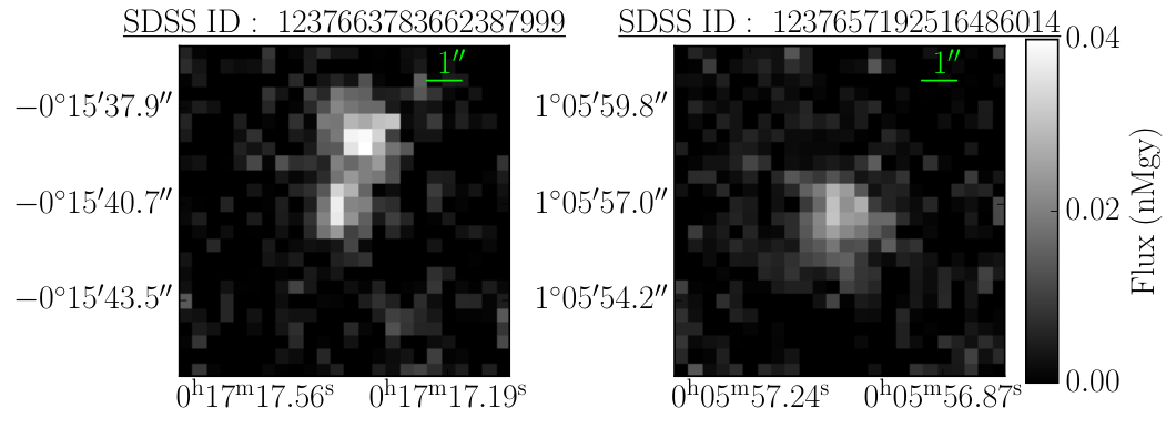
Some fits are unsuccessful because of poor image quality. In some cases the galaxy is found in a region of significantly higher noise and in other cases the galaxy is too faint. Both of these effects lead to a host intensity within a few percent of the background. Examples of these cases are shown in Fig. 3. SNIae associated with a host galaxy that could not be fit are removed from the sample. Of the 368 host galaxy images, 66 cannot be successfully fit, leaving a sample of 302 SNIae for our analysis.
We checked our sample for any biases that may have been introduced by removing the poor fits; for example, it might be expected that higher redshift galaxies on average are fainter and thus tend to be more difficult to fit. In Fig. 4 we plot histograms of the stretch, colour and redshift (the 3 parameters which are relevant to cosmology and which we use in the following section) of the complete SDSS host galaxy sample, compared with the hosts that were successfully fit. We see that the shapes of the distributions remain virtually unaffected, which is compatible with the hypothesis that removing poor fits does not introduce bias to the distributions.
Historically, spiral galaxies have been identified with a Sérsic index (corresponding to a typical exponential disc galaxy) and elliptical galaxies with a Sérsic index (de Vaucouleurs, 1959, a de Vaucouleur profile; see e.g.). More recently, it has become standard to allow to vary freely, as there is significant spread around these integer values in modern surveys (Ravindranath et al., 2004; Trujillo et al., 2006; Buitrago et al., 2008; van Dokkum et al., 2010; van der Wel et al., 2012; Vika et al., 2015, e.g.,). Fig. 5 shows the distribution of the inferred Sérsic index for both sub-groups. The mode of the group is , while the mode of the group is . We observe that we have very few galaxies with and none with . This result is consistent with the findings of Paulino-Afonso et al. (2017), who found that the reconstructed Sérsic indexes of 2507 local and 1118 high- star-forming galaxies are biased low by about 20%, almost independently of redshift. They attributed this phenomenon to cosmological dimming, leading to decreased resolution and increased noise that produces a bias towards disk-like (i.e. ) profiles. Nevertheless, we do not believe that this effect leads to a bias in our inferred values for the galactocentric distance, as explained in the next section.
2.3 Sub-groups of SNIae based on galactocentric distance to host
From our best-fit parameters we compute the projected distance of the SNIa from its host galaxy with Eq. (4):
| (11) |
where are the coordinates of the SNIa in each host galaxy image determined from our fits (which generally compare well with the coordinates in Sako et al. 2014), converted from standard RA/DEC coordinates with the AstroPy library for Python (Astropy Collaboration et al., 2013) which includes World Coordinate System (WCS) transformation functions (Calabretta & Greisen, 2002). This is the distance between an SNIa and its host galaxy if the SNIa were moved along an isophote contour to line up with the semi-major axis of the host. The galactocentric distance is obtained by dividing this distance by the scale length, :
| (12) |
This definition of galactocentric distance is a good description of the SNIa to host galaxy distance as it takes into account the geometry of the light distribution of the host galaxy, which is assumed to be a proxy for the dust that is the main contributor to SNIae extinction.
The galactocentric distance defined in Eq. (12) takes into account ellipticity and is normalized to the scale length . By contrast, Sako et al. (2014) defined galactocentric distances using circular Petrosian half-light radii instead, making a direct comparison between our two methods difficult.
In Fig. 6 we show the galactocentric distances found for our sample of 302 galaxies as a function of redshift, where the uncertainties were estimated by calculating the 68% credible intervals of the marginal posterior distributions resulting from ProFit’s MCMC. We took into account the uncertainty of the SNIa positions during the fit by drawing their right ascensions and declinations from a Gaussian distribution with a width of 0.2 pixels, the typical pointing uncertainty of the SDSS telescope (Gunn et al., 2006). We find that the mean fractional error in our measurements is about 10 per cent. While some uncertainties are quite large – a result of poor image quality in several cases – around the value only relatively few galaxies have uncertainties that would put in question their classification in one of the two groups. Therefore we conclude that discarding such uncertainties is unlikely to lead to significant differences in the subsequent analysis.
A potential difficulty would arise if our values of galactocentric distance were correlated with the Sérsic index . Since is inversely proportional to , and is positively correlated with (see e.g. Trujillo et al. (2001)), a larger value of could correlate with a smaller value of . If this were the case, our sub-groups could be a simple reflection of different galaxy morphology, rather than galactocentric distance. However, we find no significant correlation between and . Fig. 5, showing the distribution of for both sub-groups of , demonstrates that the mode of the group is at a slightly higher value of than the mode for the group. If and were anti-correlated, the larger sub-group distribution of Sérsic indexes should peak at a lower value of , not at a higher value like we observe. Therefore we conclude that our grouping based on is not a reflection of the host galaxies’ morphology.
According to our hypothesis, SNIae further from their galactic centre (i.e., with ) should explode in a galactic environment with a smaller dust column density, and hence they should exhibit less dust absorption. Following Anderson et al. (2015a), we also expect that SNIae at large galactocentric distances ought to exhibit bluer values for the colour correction. We therefore expect the distribution of the colour correction parameter , to differ for SNIae with larger than for those with close to 0. In order to test this hypothesis, we split the sample of 302 SNIae with values into two groups, one with and the other with , where is a cut-off value.
The choice of is important in establishing the significance (or otherwise) of the effect of on . Given the distribution of in our sample, shown in Fig. 7, a larger value of is expected to give a cleaner sample (i.e., SNIae less affected by dust) but at the price of a very small sample size. On the other hand, choosing a smaller cut-off value may lead to a substantial number of SNIae with that are still affected by dust. We chose a value of for our analysis, as it is reasonable to assume a transition in the amount of dust at a galactocentric distance more than twice the value of the scale radius of the galaxy. We emphasize that we are not choosing the value of to maximize the significance of the effect, but we still a posteriori check the significance of our results as a function of and correct our test statistics for multiple testing (i.e., there is no “look elsewhere effect”), as described below.
Using the fixed choice of , we define two groups of SNIae, (i) those with (250 SNIae) and (ii) those with (52 SNIae). The distributions of stretch and colour for the two groups are shown in Fig. 8. The stretch distributions for the two groups are similar, while the group appears bluer, i.e., there are more objects with .
We use a two-sample Kolmogorov-Smirnov (KS) test to assess the statistical significance of the difference in the colour and stretch distributions of the two groups. The KS test statistic is the maximum difference between the cumulative distribution function of two empirical distributions, . Here we compare the cumulative distributions of the colour for the two groups of SNIae. is compared to a threshold value
| (13) |
where ) is an -dependent critical value and and are the numbers of objects in each of the two groups. The test is significant (at the level ) if . For , the critical level is .
To investigate the sensitivity of this result to the choice of , we evaluate as a function of for comparing the distributions of both the colour and stretch corrections in the two SNIa groups. With a significance level of , the KS test for the stretch distribution is not significant for any value . (We do not consider larger values for as the number of SNIae in the group then becomes too small.) The KS test is, however, locally statistically significant for the colour distribution for , as shown by the black points in the upper panel of Fig. 9. To account for multiple testing, we use the (conservative) Bonferroni correction, where in order to achieve a confidence level of 95 per cent one must divide by the number of tests performed. Here we have a total of 7 tests (given by the chosen values of ), thus we calculate with a significance level of . The results are shown as crosses in the upper panel of Fig. 9, and indicate that the two distributions are no longer significantly different at the 95 per cent confidence level when using the Bonferroni correction.
We investigate the choice of further using the non-parametric two-sample one-sided Mann-Whitney U test (sometimes also called the Wilcoxon rank sum test). The hypothesis we want to test is that the sub-group at greater galactocentric distances is bluer than the sub-group at smaller distances. This means that the observed colour distribution for the group should be shifted to the left with respect to the distribution for the group. This translates into a one-sided hypothesis test. Let denote a SNIa drawn at random from the group, and denote a SNIa drawn at random from the group. We use the Mann-Whitney U statistic to test the one sided null hypothesis that has a smaller observed colour correction value, , than with probability greater than or equal to 0.5 against the alternative hypothesis that this probability is less than 0.5. If the null hypothesis is rejected (at a given confidence level), this means that the data indicate that the distribution of the colour correction in the group is to the left of (smaller than) this distribution of the group. This test does not require the colour correction to be normally distributed in the two groups. The one-sided Mann-Whitney U test is generally more powerful than the KS test, and it can detect differences in the shapes of the distributions, not just in their medians (as sometimes incorrectly stated). We show the resulting -values for testing the null hypothesis as a function of in the lower panel of Fig. 9. The top dashed line corresponds to a -value of 0.05, while the bottom dashed line corresponds to a Bonferroni-corrected -value of 0.05/7. P-values below these lines indicate that the null hypotheses can be rejected at the (local or global) 95 per cent confidence level. We observe that at the Mann-Whitney test indicates that the SNIae in the group have a smaller colour correction distribution than do those in the group. This holds at the 95 per cent confidence level even when the Bonferroni correction is taken into account, in contrast to the KS test.
3 Evaluating the residual scatter
After the empirical colour and stretch corrections, SNIae still exhibit a residual scatter in their (standardized) intrinsic magnitudes. Reducing this scatter enables more precise estimation of the cosmological parameters, since it allows for a more precise measurement of the distance modulus as a function of redshift. Here we turn to the question of whether there is a statistically significant difference between the magnitude of the residual scatter in the two subgroups defined in Section 2.3. We use the Bayesian hierarchical framework BAHAMAS (March et al., 2011; Shariff et al., 2016) to estimate the residual scatter of the two groups. This fully Bayesian approach is different from the classical approach in two fundamental ways.
Firstly, for each observed variable a latent (true) unobserved value is introduced using a hierarchical representation of the probabilistic relationships between the latent variables, observations and population parameters. More specifically,
| (14) |
encapsulates the linear corrections to the B-band peak apparent magnitude, , captured by the SALT2 correction, namely (colour) and (stretch). Here, is the distance modulus, which depends on the SN’s redshift, , and the underlying cosmological parameters, ; are regression coefficients to be estimated, and is the residual absolute magnitude after empirical corrections. More specifically, the SALT2 colour parameter is defined as , where all colours are evaluated at the time of B-band maximum and is the colour averaged over the SNIae in the templates (Guy et al., 2007). A value of means that the blue band magnitude is smaller (i.e., brighter) than the band, hence the object is bluer. On the other hand, means the object is redder (than average). Unlike in the approach, in BAHAMAS are latent variables that are stochastically related to their observed counterparts, but differ from the data because of observational noise. Since the SNIae in our data are spectroscopically confirmed, the errors in redshift can be ignored. The redshift range of the SNIae used in this analysis is restricted by the need to acquire host galaxy images, and spans . With this narrow range, SNIa data alone cannot constrain the cosmological parameters. We therefore assume a flat CDM universe with a fixed cosmology, , matching the posterior mean value obtained by the Planck Cosmic Microwave Background mission (Planck Collaboration et al., 2015).
The second key feature of the Bayesian approach is its ability to account for population variability. Instead of assuming that each SNIa has the same absolute magnitude (after corrections), we assume that they vary probabilistically with an underlying population-level distribution. Specifically, we model the residual absolute magnitude, , using a Gaussian distribution:
| (15) |
where is the mean of the residual absolute magnitudes and is its residual standard deviation, quantifying the residual scatter of SNIae after corrections. This quantity is to be understood as a phenomenological error describing the intrinsic residual variability that is not accounted for by the empirical corrections for stretch and colour.
It was demonstrated by March et al. (2011) with simulated data that (a precursor of) the Bayesian approach used in BAHAMAS results in less biased, more accurate estimates than the standard approach, while improving overall coverage of the ensuing credible intervals. We apply BAHAMAS to the two SNIa groups ( and ), as well as to the whole dataset for comparison, and obtain the marginal posterior distribution of numerically using the sampler presented in Shariff et al. (2016). Full details of BAHAMAS, including prior choices, hierarchical structure and the sampling algorithms are given in Shariff et al. (2016).
Our approach to estimating the residual scatter, and the colour and stretch corrections parameters is significantly more sophisticated than what has been adopted in previous works attempting to establish the influence of galactocentric distance (Ivanov et al., 2000; Galbany et al., 2012). The Bayesian method adopted here has the advantage of exploiting the probabilistic nature of the model to ‘borrow strength’ between SNIae, thus increasing sensitivity to subtler features in the data than relative to the cruder approach. Furthermore, we produce a full marginal probability distribution for the value of the intrinsic scatter, not just a point estimate. As shown in March et al. (2011) this results in more accurate and precise estimates for the parameters of interest than it is possible with the standard method.
In the present work we segregate SNIae according to the two sub-groups defined above. Alternatively, one could include as an additional linear covariate in the correction term in Eq. (14), the slope of which would be another free parameter, thus replacing Eq. (14) with:
| (16) |
where and , with the slope of the galactocentric distance covariate. One would then fit the value of together with the colour and stretch correction coefficients, and . The inclusion of galactocentric distance as an additional standardization variable is akin to how the host galaxy mass correction is usually parameterized. In both cases, one can either segregate the SNIae in two groups, divided by a cut-off value, or use the additional covariate as a linear correction term in the distance modulus, as was done e.g., in Shariff et al. (2016). The second approach dispenses with the need of defining an arbitrary cut-off point.
In previous studies, Ivanov et al. (2000); Galbany et al. (2012) investigated the impact of galactocentric distance as a covariate. Galbany et al. (2012) also used only two bins (‘near’ and ‘far’). Importantly, the ‘near’ and ‘far’ bins were defined by splitting the SNIae into two groups of equal size (and further subdividing them according to host morphology), and not with reference to their normalized galactocentric distance, like we do here. This might have washed out any potential correlation. A puzzling result of Galbany et al. (2012) is that while decreased with distance (with a reported significance of the correlation coefficient of 4.4) for the entire data set, the effect disappeared when the data were split according to morphology. Yasuda & Fukugita (2010) also adopted (de-projected) galactocentric distance as a covariate, finding no effect. They, however, did not attempt to normalize the galactocentric distance to the host light radius, as we do here.
For simplicity, we only consider splitting the SNIae into two groups (with a hard, pre-defined cut), and leave investigation of the galactocentric distance as a linear covariate to future work.
4 Results
The marginal posterior distributions in one and two dimensions for the parameters of interest, are shown in Fig. 10, split according to sub-group and compared with the result for the whole data set. Table 2 gives posterior summary statistics for the same quantities. In both cases, the latent parameters (, where is the number of SNIae considered) and all other population-level parameters, , have been marginalized out. Here, and are the (redshift-independent) population means of the colour and stretch distributions, respectively, and are their variances. The distributions of colour and stretch are taken to be Gaussian, see Shariff et al. (2016) for full details.
| All data | |||
|---|---|---|---|
We observe shifts in the distributions of the all quantities for the two different sub-groups. The most dramatic difference is in the value of the residual scatter, . Its posterior distribution is fairly Gaussian, and has posterior average and standard deviation given by for the sub-group, which is reduced to for the sub-group. This represents a reduction of per cent in the posterior mean values. The significance of the difference is approximately 2.0 (computed using the standard deviation of the difference between in the two subgroups and assuming Gaussian errors). While this is not strongly significant, we emphasize the small sample size ( for the sub-group), which results in a fairly wide posterior distribution for . This means that SNIae at large galactocentric distances show better standardization properties (i.e., are more uniform in their magnitudes after corrections) than the whole data set. This is additionally supported by Fig. 11, showing the Hubble residuals of the two sub-groups. The right/blue () residuals are clearly smaller than the left/red ones (). SNIae further away from the centre of the galaxy have, on average, smaller residuals after corrections. Therefore, cosmological distance estimation from this sub-group can be expected to be more precise.
We show in Figures 12 and 13 the inferred posterior mean and standard deviation for the latent colour and (post-correction) intrinsic magnitude for each SNIa, fit separately for the two subgroups. Fig. 12 shows that indeed the sub-group has a latent colour distribution that is skewed towards bluer objects (we note that this result still holds even for the observed colours, albeit with a larger scatter). From Fig. 13 we observe that the sub-group distribution of intrinsic magnitudes is tighter. The difference in mean absolute magnitude (post-correction) between the two groups is , so compatible with zero. Therefore, we conclude that there is no evidence for a difference in the average, post-correction magnitudes in the SNIae between the two sub-groups.
One could imagine that the physical explanation for our findings might lie in the reduced amount of dust found at high galactocentric radii: since the observed colour variation is the sum of intrinsic colour variability and reddening due to the host galaxy and/or local circumstellar material (CSM) dust (which varies from host to host), reducing the host galaxy colour variability should lead to a smaller residual scatter after correction, as observed in our results. However, this interpretation is at odds with the inferred value of the colour correction coefficient for the sub-group (), which is larger than for the sub-group (). Owing to the larger uncertainty in the value for the sub-group (which contains a smaller number of SNIae), the difference is not statistically significant. However, the fact that the sub-group has a larger posterior mean for cannot be reconciled with the notion that high galactocentric distance SNIae are subject to reduced host galaxy reddening, for the following reason.
There is evidence (Wang, 2005; Goobar, 2008) that the local CSM might have smaller size dust grains (compared to the Milky Way), leading to a smaller value of the total-to-selective extinction than the average Milky Way value of . Here, is the extinction (in mag) in band , i.e., , where is the apparent magnitude in band and is the apparent magnitude in the same band in the absence of extinction. The colour excess is given by . Given that total extinction and reddening is the cumulative effect of local CSM dust and ISM dust, if the effect of the ISM were largely removed by the cut to large , one would expect this sub-group to exhibit the reddening law of the underlying CSM, which is typically steeper22 2 The wavelength dependency of extinction in the vicinity of the band is approximately linear in with slope , where is the wavelength (Cardelli et al., 1989). Hence a smaller value of results in a steeper reddening law. than the Milky Way value. For example, for SN2014J Yang et al. (2016) found evidence of a luminous arc – attributed to the CSM – with an estimated . Recall that, from Eq. (14), is the slope that gives the change in band magnitude for a unit change in the value of . Therefore, ought to be compared to . Given their respective definitions, it follows that , hence . From this, one would expect that reddening due to the CSM should typically show , i.e., a much smaller value than we observe in the sub-sample, for which .
Alternatively, in the absence of CSM reddening one would expect the inferred value of for the sub-sample to recover the value associated with the intrinsic colour variability of the SNIae. This has been estimated by Mandel et al. (2016) in a low-redshift sample, finding , again much lower than the value we obtain for our sub-sample at high galactocentric distance. Mandel et al. (2016) argue that the simple linear colour correction formula (which we adopt in this work, in line with standard usage) effectively averages between the intrinsic colour correction, , and the reddening law slope. Thus one would expect that if indeed the sub-group had negligible reddening due to the ISM, we would observe a value of that averages between the value found by Mandel et al. (2016) and the CSM reddening law, equivalent to . Thus the inferred for the sub-group ought to be around 2.2, which is not what we observe.
Folatelli et al. (2010) analysed the first set of low-redshift SNIae from the Carnegie Supernovae Project (CSP), and found ( for the entire set of SNIae. However, when excluding two highly reddened SNIae from their analysis, they obtained (. While their value is somewhat higher than our value for the sub-group (), the effect goes in the same direction. Our value for for the larger galactocentric distance sub-group however still falls short of the average Milky Way value of (corresponding to ). More recently, Burns et al. (2014) used the late-time Lira (1996) law to select a low-reddening sample of 34 SNIae from the Carnegie Supernovae Project (CSP). Their approach circumvents the use of galactocentric distance, which can be expected to assign to the sub-group SNIae that are low reddened but at small projected radii (i.e., in front of the host). Burns et al. (2014) then employed a Bayesian hierarchical model to reconstruct the reddening law of the host (under a number of priors). They found that objects with the least reddening () have a reddening law compatible with the Milky Way value of (corresponding to ). This is compatible with our observation of a shift of to larger values in the group, which (being the bluer sub-group) exhibits the least reddening. This thus hints at the possibility that the shift of to higher values for the sub-group is compatible with the hypothesis that the remaining reddening is due to the host ISM. Furthermore, despite not finding any correlation between colour and galactocentric distance, Yasuda & Fukugita (2010) do observe an excess of redder colour values at low galactocentric distances, compatible with the later findings of Anderson et al. (2015b). Another heuristic (if counterintuitive) argument in support of our findings comes from the fact that less massive galaxies (with stellar mass ) show a larger value of (Sullivan et al., 2010). These galaxies are also the ones with the least dusty environments (Garn & Best, 2010). Hence a larger value of can be associated with less dusty environments.
Taken all together, the above arguments lend credence to the hypothesis that the large sub-group is actually probing a low-reddening/low-attenuation ISM environment, rather than seeing the underlying CSM/intrinsic colour scatter. The reduction in residual intrinsic scatter we observe could be the resultant of the sub-group being subject to a less dusty ISM, as well as to the more homogeneous metallicity and SFR environment for this sub-group. Further work is required to disentangle the physical origin of this effect, and we comment on this aspect in the next section.
In this work we have not divided hosts in terms of their morphology. Since early-type galaxies are dominated by old stars and relatively dust-free (Wise & Silva, 1996), while spirals have star-forming activity in the arms and a diverse (age-wise) stellar population, SNIae that occur in early-type galaxies are less likely to be significantly affected by dust. In spirals, central stars tend to be both older and metal rich than in outer regions, and therefore classifying SNIae according to both radial distance and galaxy type could potentially disentangle the effects due to stellar age and metallicity from those due to dust properties. One might therefore speculate that including host galaxy morphology information could help in further reducing the residual scatter, and perhaps in clarifying the origins of the effect. Lampeitl et al. (2010) subdivided the SDSS-II SNIa sample in two groups, according to the passive or star forming nature of their host galaxies (based on their estimated SFR). They found a strong difference in the stretch parameter, , for the two groups, but no significant difference in the colour, concluding that SNIae must have the same intrinsic colour variations in all galaxy types. This conclusion was confirmed by Henne et al. (2017), who examined the influence of galaxy morphology by classifying hosts in three groups – ellipticals/lenticulars (E,S0), early-type spirals (Sa-Sc), late-type spirals (Sd-Ir)– for 192 SNIae from JLA. While they reported 1 shifts in the reconstructed values of depending on galactic morphology group, they did not find any significant correlation between colour and host morphology. This conclusion stood despite a weak trend of slightly bluer colour SNIae in early type (i.e., passive) hosts. This was interpreted as being due to the larger amount of dust in spirals, which would thus make the SN colour redder. The above studies thus seem to suggest that our results are not strongly affected by the lack of morphological host information.
Even the spectroscopic SDSS-II SN sample is known to be complete only out to (Sako et al., 2018), and we have used SNIae out to . As the apparent magnitude of high- SNIae approaches the flux limit of the telescope, brighter objects will be detected preferentially, leading to a bias in their inferred distance modulus. The sub-group has on average smaller colour values, and an inferred larger value than the group, which means that the colour correction term in Eq. (14) for the sub-group is (at a given redshift) more negative than for the sub-group. It follows from Eq. (14) that at a fixed redshift (and thus fixed value of ) the apparent magnitude for the sub-group is on average smaller than for the sub-group (since there are no significant differences in either or between the two groups, as shown in Figures 8 and 13). Hence for SNIae in the sub-group can be expected to have a larger apparent brightness and therefore might be preferentially selected due to magnitude-based selection effects. When plotting the ratio of the number of SNIae in the sub-group to the sub-group as a function of redshift, we do observed an increase for . However, due to the smaller number of objects at larger redshift, the Poisson uncertainty in the ratio is quite large, and the increase in the ratio is not statistically significant. Furthermore, when considering the Hubble residuals as a function of for the two subgroups, we do not observe any feature in their distribution (like a skewness, which would be indicative of residual selection effects) above . Therefore, we conclude that magnitude-based selection effects do not play a statistically significant role in our results.
This work does not consider colour-based selection effects over and above the (magnitude) corrections already implemented in the JLA sample. There is evidence that high- SNIa are bluer (Rubin & Hayden, 2016) and come from less dusty environment (Mandel et al., 2016) due to selection bias. However, our sub-group spans almost the entire SDSS-SNIa redshift range (see Fig. 7), with the majority of the SNIae at , and hence colour-based selection effects are unlikely to be playing a major role here.
5 Conclusions
We have measured the projected galactocentric distance to the host of the SNIae for a sub-set of the SDSS Type Ia SNIae in the JLA sample and investigated the scatter around the Hubble diagram (for a fixed cosmology) for two sub-groups, separated by a cut in their distance. The rationale was that SNIae at large galactocentric distances might be less subject to ISM reddening and absorption, and might explode in more homogeneous environments in terms of metallicity and local SFR.
We have demonstrated that SNIae further away from the host can be standardized to a higher degree, in that their intrinsic dispersion (post stretch and colour corrections) is reduced from (for the full sample) to (for the SNIae with larger galacocentric distances). The statistical significance of the effect is, however, small (about ). This is primarily due to the smallness of the sample (only 49 SNIae in the sub-group). Future surveys and data tabulations should be encouraged to include measured galactocentric distances (and, perhaps, morpholgy of host) to account for this effect. In a Bayesian framework, it would be straightforward to include prior information on extinction and reddening depending on galactocentric distance and morphology of host. This has the potential to improve accuracy and precision for inferred cosmological parameters.
Future work should focus on verifying whether a larger sample size can confirm this tentative result. The SDSS-II SN sample contains a larger number of photometrically observed SNIa, which have not been included in this analysis. Campbell et al. (2016) analysed 721 SNIae from this larger data set, and used different host properties such as age and metallicity to reduce the Hubble residual. Given the availability of SDSS imagery for the hosts, the additional supernovae in the photometric SDSS sample could be analyzed to corroborate or disprove this result. Also, since this is a photometric sample, there is a possibility of contamination of the sample by non-SNIa’s. A Bayesian supernova classifier (Hlozek et al., 2012; Jones et al., 2016; Revsbech et al., 2017) can be used to account for this. Additionally, since this photometric sample contain SNIa to a higher redshift, selection effects may play a major role and have to be correctly accounted for (e.g. as in Rubin et al. 2015). Another, complementary low-redshift () SNIae sample is the one used in Mandel et al. (2016), from a compilation of data including high-quality light curves from the CfA and CSP surveys. An advantage of this lower redshift data set is that detailed morphological studies can be carried out on these relatively nearby galaxies, to verify whether or not host galaxy type plays a role in the correction procedure. Furthermore, the source of the difference in value from the two sub-groups could be elucidated by analyzing them with the SIMPLE-BayeSN framework (Mandel et al., 2016). The upcoming SNIa data from the Dark Energy Survey would also be a very useful testing ground for our method. We leave exploration of all these avenues to future work.
Acknowledgements: we dedicate this paper to the memory of our colleague and co-author, L.B. Lucy (1938-2018). We thank Heather Campbell, Kaisey Mandel and Marc Sullivan for useful discussions. We are grateful to an anonymous referee for helpful suggestions and comments that have improved this work. This work was supported by Grant ST/N000838/1 from the Science and Technology Facilities Council (UK). RT was partially supported by an EPSRC “Pathways to Impact” grant. RT, DvD, and HS were supported by a Marie-Skodowska-Curie RISE (H2020-MSCA-RISE-2015-691164) Grant provided by the European Commission.
References
- Ahn et al. (2014) Ahn C. P., et al., 2014, ApJS, 211, 17
- Amanullah et al. (2010) Amanullah R., et al., 2010, ApJ, 716, 712
- Anderson et al. (2015a) Anderson J. P., James P. A., Habergham S. M., Galbany L., Kuncarayakti H., 2015a, Publ. Astron. Soc. Australia, 32, e019
- Anderson et al. (2015b) Anderson J. P., James P. A., Förster F., González-Gaitán S., Habergham S. M., Hamuy M., Lyman J. D., 2015b, MNRAS, 448, 732
- Astier et al. (2006) Astier P., et al., 2006, A&A, 447, 31
- Astropy Collaboration et al. (2013) Astropy Collaboration et al., 2013, ApJ, 558, A33
- Bailey et al. (2008) Bailey S., et al., 2008, preprint, (arXiv:0810.3499)
- Balland et al. (2009) Balland C., et al., 2009, A&A, 507, 85
- Betoule et al. (2014) Betoule M., et al., 2014, A&A, 568, A22
- Branch et al. (1993) Branch D., Fisher A., Nugent P., 1993, AJ, 106, 2383
- Buitrago et al. (2008) Buitrago F., Trujillo I., Conselice C. J., Bouwens R. J., Dickinson M., Yan H., 2008, ApJ, 687, L61
- Burns et al. (2014) Burns C. R., et al., 2014, ApJ, 789, 32
- Calabretta & Greisen (2002) Calabretta M. R., Greisen E. W., 2002, A&A, 395, 1077
- Campbell et al. (2013) Campbell H., et al., 2013, ApJ, 763, 88
- Campbell et al. (2016) Campbell H., Fraser M., Gilmore G., 2016, MNRAS, 457, 3470
- Cardelli et al. (1989) Cardelli J. A., Clayton G. C., Mathis J. S., 1989, ApJ, 345, 245
- Contreras et al. (2010) Contreras C., et al., 2010, ApJ, 139, 519
- D’Andrea et al. (2011) D’Andrea C. B., et al., 2011, ApJ, 743, 172
- Doi et al. (2010) Doi M., et al., 2010, AJ, 139, 1628
- Folatelli et al. (2010) Folatelli G., et al., 2010, AJ, 139, 120
- Freedman et al. (2009) Freedman W. L., Burns C. R., Phillips M., Wyatt P., Persson S., et al., 2009, ApJ, 704, 1036
- Galbany et al. (2012) Galbany L., et al., 2012, ApJ, 755, 125
- Gallagher et al. (2008) Gallagher J. S., Garnavich P. M., Caldwell N., Kirshner R. P., Jha S. W., Li W., Ganeshalingam M., Filippenko A. V., 2008, ApJ, 685, 752
- Garn & Best (2010) Garn T., Best P., 2010, MNRAS, 409, 421
- Goobar (2008) Goobar A., 2008, ApJ, 686, L103
- Gunn et al. (2006) Gunn J. E., et al., 2006, AJ, 131, 2332
- Guy et al. (2007) Guy J., et al., 2007, A&A, 466, 11
- Henne et al. (2017) Henne V., et al., 2017, New Astron., 51, 43
- Hicken et al. (2009) Hicken M., et al., 2009, ApJ, 700, 331
- Hlozek et al. (2012) Hlozek R., et al., 2012, ApJ, 752, 79
- Ivanov et al. (2000) Ivanov V. D., Hamuy M., Pinto P. A., 2000, ApJ, 542, 588
- Jha et al. (2007) Jha S., Riess A. G., Kirshner R. P., 2007, ApJ, 659, 122
- Jones et al. (2013) Jones D. O., et al., 2013, ApJ, 768, 166
- Jones et al. (2015) Jones D. O., Riess A. G., Scolnic D. M., 2015, ApJ, 812, 31
- Jones et al. (2016) Jones D. O., et al., 2016, preprint (arXiv:1611.07042)
- Kasen & Woosley (2007) Kasen D., Woosley S. E., 2007, ApJ, 656, 661
- Kelly et al. (2010) Kelly P. L., Hicken M., Burke D. L., Mandel K. S., Kirshner R. P., 2010, ApJ, 715, 743
- Kelly et al. (2015) Kelly P. L., Filippenko A. V., Burke D. L., Hicken M., Ganeshalingam M., Zheng W., 2015, Science, 347, 1459
- Kessler et al. (2009) Kessler R., et al., 2009, ApJS, 185, 32
- Kowalski et al. (2008) Kowalski M., et al., 2008, ApJ, 686, 749
- Lampeitl et al. (2010) Lampeitl H., et al., 2010, ApJ, 722, 566
- Lira (1996) Lira P., 1996, Master’s thesis, Univ. Chile (1996)
- Maeda & Terada (2016) Maeda K., Terada Y., 2016, Int. J. Mod. Phys., D25, 1630024
- Mandel et al. (2009) Mandel K. S., Wood-Vasey W. M., Friedman A. S., Kirshner R. P., 2009, ApJ, 704, 629
- Mandel et al. (2016) Mandel K. S., Scolnic D., Shariff H., Foley R. J., Kirshner R. P., 2016, preprint (arXiv:1609.04470)
- March et al. (2011) March M. C., Trotta R., Berkes P., Starkman G. D., Vaudrevange P. M., 2011, MNRAS, 418, 2308
- Moreno-Raya et al. (2016) Moreno-Raya M. E., López-Sánchez Á. R., Mollá M., Galbany L., Vílchez J. M., Carnero A., 2016, MNRAS, 462, 1281
- Paulino-Afonso et al. (2017) Paulino-Afonso A., Sobral D., Buitrago F., Afonso J., 2017, MNRAS, 465, 2717
- Perlmutter et al. (1999) Perlmutter S., et al., 1999, ApJ, 517, 565
- Phillips (1993) Phillips M., 1993, ApJ, 413, L105
- Phillips et al. (1999) Phillips M. M., Lira P., Suntzeff N. B., Schommer R. A., Hamuy M., Maza J., 1999, AJ, 118, 1766
- Planck Collaboration et al. (2015) Planck Collaboration et al., 2015, preprint, (arXiv:1502.01589)
- Ravindranath et al. (2004) Ravindranath S., et al., 2004, ApJ, 604, L9
- Rest et al. (2014) Rest A., Scolnic D., Foley R., Huber M., Chornock R., et al., 2014, ApJ, 795, 44
- Revsbech et al. (2017) Revsbech E., Trotta R., van Dyk D., 2017, in prep
- Riess et al. (1996) Riess A. G., Press W. H., Kirshner R. P., 1996, ApJ, 473, 88
- Riess et al. (1998) Riess A. G., et al., 1998, AJ, 116, 1009
- Rigault et al. (2013) Rigault M., et al., 2013, A&A, 560, A66
- Robotham et al. (2017) Robotham A. S. G., Taranu D. S., Tobar R., Moffett A., Driver S. P., 2017, Mon. Not. Roy. Astron. Soc., 466, 1513
- Rubin & Hayden (2016) Rubin D., Hayden B., 2016, preprint (arXiv:1610.08972)
- Rubin et al. (2015) Rubin D., et al., 2015, ApJ, 813, 137
- Sako et al. (2014) Sako M., et al., 2014, preprint (arXiv:1401.3317)
- Sako et al. (2018) Sako M., et al., 2018, PASP, 130, 064002
- Scovacricchi et al. (2016) Scovacricchi D., Nichol R. C., Macaulay E., Bacon D., 2016, preprint (arXiv:1611.01315)
- Sérsic (1963) Sérsic J. L., 1963, Argentina Bol., 6, 41
- Shariff et al. (2016) Shariff H., Jiao X., Trotta R., van Dyk D. A., 2016, ApJ, 827, 1
- Smith et al. (2014) Smith M., et al., 2014, ApJ, 780, 24
- Sternberg et al. (2011) Sternberg A., et al., 2011, Science, 333, 856
- Sullivan et al. (2006) Sullivan M., et al., 2006, ApJ, 648, 868
- Sullivan et al. (2010) Sullivan M., et al., 2010, MNRAS, 406, 782
- Suzuki et al. (2012) Suzuki N., et al., 2012, ApJ, 746, 85
- Trujillo et al. (2001) Trujillo I., Graham A. W., Caon N., 2001, MNRAS, 326, 869
- Trujillo et al. (2006) Trujillo I., et al., 2006, ApJ, 650, 18
- Vika et al. (2015) Vika M., Vulcani B., Bamford S. P., Häußler B., Rojas A. L., 2015, A&A, 577, A97
- Wang (2005) Wang L., 2005, ApJ, 635, L33
- Wise & Silva (1996) Wise M. W., Silva D. R., 1996, ApJ, 461, 155
- Wood-Vasey et al. (2007) Wood-Vasey W. M., Miknaitis G., Stubbs C. W., 2007, ApJ, 666, 694
- Yang et al. (2016) Yang Y., et al., 2016, preprint (arXiv:1610.02458)
- Yasuda & Fukugita (2010) Yasuda N., Fukugita M., 2010, AJ, 139, 39
- de Vaucouleurs (1959) de Vaucouleurs G., 1959, Handbuch der Physik, 53, 311
- van Dokkum et al. (2010) van Dokkum P. G., et al., 2010, ApJ, 709, 1018
- van der Wel et al. (2012) van der Wel A., et al., 2012, ApJS, 203, 24