跳到论文正文
W Papers独立论文阅读器 arXiv:1612.04362 论文正文 计算阅读时间 · 0%
引用这篇论文根据当前论文元数据生成,正式投稿前建议核对。


License: arXiv.org perpetual non-exclusive license
arXiv:1612.04362v1 [astro-ph.GA] 13 Dec 2016

Laboratory Frequency Redistribution Function forthe Polarized Λ\Lambda-Type Three-Term Atom

The National Center for Atmospheric Research is sponsored by the National Science Foundation.
R. Casini1 and R. Manso Sainz2 Affiliation: 1High Altitude Observatory, National Center for Atmospheric Research,P.O. Box 3000, Boulder, CO 80307-3000, U.S.A. Affiliation: 2Max Planck Institute for Solar System Research,Justus-von-Liebig-Weg 3, 37077 Göttingen, Germany
Abstract

We present the frequency redistribution function for the polarized three-term atom of the Λ\Lambda-type in the collisionless regime, and we specialize it to the case where both the initial and final terms of the three-state transition are metastable (i.e., with infinitely sharp levels). This redistribution function represents a generalization of the well-known RIIR_{\rm II} function to the case where the lower terms of the transition can be polarized and carry atomic coherence, and it can be applied to the investigation of polarized line formation in tenuous plasmas, where collisional rates may be low enough that anisotropy induced atomic polarization survives even in the case of metastable levels.

I. Introduction

Plasma diagnostics in both laboratory and astrophysical settings relies principally on spectroscopic and polarimetric methods of observation, where the radiation emitted from the plasma is analyzed as a function of wavelength and state of polarization. These allow one to determine important properties of the observed plasma, such as bulk and turbulent velocity fields, gas composition and density, existence of anisotropic processes such as the presence of directed electric and/or magnetic fields, and anisotropic sources of irradiation and of colliding particles.

Particularly in the case of low density gases, collisional processes can be of such modest magnitude that the excitation state of the plasma is typically far away from local thermodynamical equilibrium (LTE). In that case, the excitation and de-excitation processes that are responsible for the observed radiation may be statistically correlated, so that the system is able to preserve a “memory” of the excitation conditions. A typical example is the partially coherent scattering of radiation, where the frequency of the outgoing photon is correlated (via an intrinsically second-order atom–photon process) to the spectral distribution of the incoming radiation, leading to the phenomenon of partial redistribution of frequency.

These excitation conditions are rather common in low-density astrophysical plasmas, such as the higher layers of the solar atmosphere, planetary nebulae, and interstellar H I regions, where outstanding spectral lines of the observed spectrum (e.g., the first few lines of the Lyman and Balmer series of hydrogen, some lines of neutral sodium, and of singly ionized calcium, etc.) are known to be formed in conditions of strong departure from LTE, which may often also include the effects of partially coherent scattering of radiation.

In this paper, we derive the redistribution function in the laboratory frame for the polarized three-term atom of the Λ\Lambda-type, i.e., for the transition system (l,l′)→(u,u′)→f(l,l^{\prime})\to(u,u^{\prime})\to f such that l,l′,f≺u,u′l,l^{\prime},f\prec u,u^{\prime} by energy ordering (see Figure 1). This model can be used to investigate, for example, the formation of the Ca II system of transitions comprising the K and H lines and the infrared (IR) triplet of the solar spectrum [3].

The expression we arrive at corresponds to the extension of the well-known RIIR_{\rm II} redistribution function [10, e.g.,] to the case of a three-term atom that can harbor atomic polarization in all of its levels, including those of the lower (metastable) states. In applications where plasma collisions are important in determining the statistical equilibrium of the atomic system, this expression is still useful as it provides the correct contribution to the total emissivity of the plasma from radiation scattering. As long as the collisional lifetime of the metastable states is much longer than the total lifetime of the upper state, the approximation of sharp lower levels remains applicable in practice, and our expression of RIIR_{\rm II} can then be used, with proper weights, alongside with RIIIR_{\rm III}, to completely describe the radiative and collisional redistribution of radiation in the modeled atmosphere [2, see, e.g.,].

Refer to caption
Figure 1.— Schematic diagram for the fluorescent scattering in a three-term model atom of the Λ\Lambda-type, for an incoming photon of frequency ωk\omega_{k} and an outgoing photon of frequency ωk′\omega_{k^{\prime}}. The model atom considered in this paper is restricted to the case where all (l,l′)(l,l^{\prime}) and ff levels are sharp (i.e., metastable). However, all the levels involved can be non-degenerate.

II. The redistribution function for the Λ\Lambda-type three-term atom

We rely on previously published work [4, hereafter, Paper I] on the redistribution function for the polarized two-term atom in order to develop the framework for the generalization of RIIR_{\rm II} to the case of a three-term atom of the Λ\Lambda-type, undergoing the two-photon transition (l,l′)→(u,u′)→f(l,l^{\prime})\to(u,u^{\prime})\to f (see Figure 1). The bases for this generalization were laid out in a recent paper [3], where we showed how the radiative transfer equation describing the polarized line formation in a two-term atom in the presence of partially coherent scattering (Equations (19) and (20) of Paper I) naturally extends to the case of the multi-term atom of the Λ\Lambda-type (Equations (1) and (2) of Casini & Manso Sainz 3).

In practice, the main complication in deriving the redistribution function for the three-term atom comes from allowing ϵf≠ϵl,l′\epsilon_{f}\neq\epsilon_{l,l^{\prime}} for the final state ff (here ϵa\epsilon_{a} is the total width of the level aa due to all possible relaxation processes), and from the need to assume generally different thermal widths for the two transitions l→ul\to u and u→fu\to f. Accordingly, we introduce a characteristic Doppler width Δm​n\Delta_{mn} for the atomic transition between two generic terms mm and nn with energy EmE_{m} and EnE_{n}, respectively. We indicate with ωm​n=(Em−En)/ℏ\omega_{mn}=(E_{m}-E_{n})/\hbar the Bohr frequency of such transition.

For each scattering event, the angle Θ\Theta between the propagation directions of the incoming and outgoing photons is an essential parameter of the laboratory frame redistribution function. We introduce the associated quantities

C=cos⁡Θ,S=sin⁡Θ,C=\cos\Theta\;,\qquad S=\sin\Theta\;, (1)

and follow [6] for the choice of the Cartesian reference frame for the projection of the thermal velocity of the plasma. This coincides with the frame adopted in Paper I [10, see also] when the thermal widths of the two transitions are identical (i.e., when the terms ll and ff have the same energy). Accordingly, we define for the Λ\Lambda-type transition l→u→fl\to u\to f,

Δ=(Δu​l2+Δu​f2−2​C​Δu​l​Δu​f)1/2,\Delta=(\Delta_{ul}^{2}+\Delta_{uf}^{2}-2C\Delta_{ul}\Delta_{uf})^{1/2}\;, (2)
ξl=Δu​l/Δ,ξf=Δu​f/Δ.\xi_{l}=\Delta_{ul}/\Delta\;,\qquad\xi_{f}=\Delta_{uf}/\Delta\;. (3)

We note that Equations (2) and (3) imply

ξl2+ξf2−2​C​ξl​ξf=1.\xi_{l}^{2}+\xi_{f}^{2}-2C\xi_{l}\xi_{f}=1\;. (4)

We define next the complex profile function [7, e.g.,]

W⁡(v,a)\displaystyle W(v,a) ≡\displaystyle\equiv 1π​∫−∞+∞d​p​e−p2a+i⁡(p−v)=exp⁡(a−i​v)2​erfc​(a−i​v)\displaystyle\frac{1}{\pi}\int_{-\infty}^{+\infty}dp\;\frac{{\rm e}^{-p^{2}}}{a+{\rm i}(p-v)}=\exp(a-{\rm i}v)^{2}\,\mbox{erfc}(a-{\rm i}v) (5)
≡\displaystyle\equiv H⁡(v,a)+i​L​(v,a),\displaystyle H(v,a)+{\rm i}\,L(v,a)\;,

where erfc(z) is the complementary error function [1, e.g.,], and H⁡(v,a)H(v,a) and L⁡(v,a)L(v,a) are respectively the Voigt and Faraday–Voigt functions, along with the dimensionless frequency variables

vm​n=(ω^k−ωm​n)/Δ,wm​n=(ω^k′−ωm​n)/Δ.v_{mn}=(\hat{\omega}_{k}-\omega_{mn})/\Delta\;,\qquad w_{mn}=(\hat{\omega}_{k^{\prime}}-\omega_{mn})/\Delta\;. (6)

The incoming and outgoing radiation frequencies, ω^k\hat{\omega}_{k} and ω^k′\hat{\omega}_{k^{\prime}}, are expressed in the laboratory frame of reference, and they differ from the corresponding frequencies in the atomic frame of rest because of the thermal motion of the atoms (see Appendix of Paper I). We also introduce normalized damping parameters associated with the inverse lifetimes of the transition levels, using the same “reduced” Doppler width of Equation (2)

am=ϵm/Δ.a_{m}=\epsilon_{m}/\Delta\;. (7)

In the presence of pressure broadening, the numerator of Equation (7) should be augmented by the corresponding collisional inverse lifetime.

We note in passing that the proposed normalizations (6) and (7) differ from the one adopted in Paper I, where instead the frequency and inverse lifetimes pertaining to a given transition were normalized to the Doppler width for that transition. The choice adopted here is dictated exclusively by convenience, as it significantly simplifies the form of the resulting expressions.

Following the approach of Paper I, Appendix A, we find that we can perform the integration over two of the three components of the thermal velocity in the adopted reference frame. Accordingly, after some algebra, the redistribution function of the polarized three-term atom of the Λ\Lambda-type can be written in the following integral form

R⁡(Ωu,Ωu′,Ωl,Ωl′,Ωf,ω^k,ω^k′,Θ)\displaystyle R(\Omega_{u},\Omega_{u^{\prime}};\Omega_{l},\Omega_{l^{\prime}},\Omega_{f};\hat{\omega}_{k},\hat{\omega}_{k^{\prime}};\Theta) =\displaystyle= 1Δ2​S​ξl​ξf​∫−∞+∞d​q​e−q2\displaystyle\frac{1}{\Delta^{2}\,S\xi_{l}\xi_{f}}\int_{-\infty}^{+\infty}dq\;{\rm e}^{-q^{2}} (8)
×{W⁡(vu​l′+q⁡(C​ξl​ξf−ξl2)S​ξl​ξf,au+al′S​ξl​ξf)al′+af+i⁡(q−vu​l′+wu​f)+W¯​(vu′​l+q⁡(C​ξl​ξf−ξl2)S​ξl​ξf,au′+alS​ξl​ξf)al+af−i⁡(q−vu′​l+wu′​f)\displaystyle\kern-158.99377pt\times\Biggl\{\frac{W\bigl(\frac{v_{ul^{\prime}}+q(C\xi_{l}\xi_{f}-\xi_{l}^{2})}{S\xi_{l}\xi_{f}},\frac{a_{u}+a_{l^{\prime}}}{S\xi_{l}\xi_{f}}\bigr)}{a_{l^{\prime}}+a_{f}+{\rm i}\bigl(q-v_{ul^{\prime}}+w_{uf}\bigr)}+\frac{\overline{W}\bigl(\frac{v_{u^{\prime}l}+q(C\xi_{l}\xi_{f}-\xi_{l}^{2})}{S\xi_{l}\xi_{f}},\frac{a_{u^{\prime}}+a_{l}}{S\xi_{l}\xi_{f}}\bigr)}{a_{l}+a_{f}-{\rm i}\bigl(q-v_{u^{\prime}l}+w_{u^{\prime}f}\bigr)}
+W⁡(wu​f+q⁡(ξf2−C​ξl​ξf)S​ξl​ξf,au+afS​ξl​ξf)al+af−i⁡(q−vu​l+wu​f)+W¯​(wu′​f+q⁡(ξf2−C​ξl​ξf)S​ξl​ξf,au′+afS​ξl​ξf)al′+af+i⁡(q−vu′​l′+wu′​f)\displaystyle\kern-158.99377pt\,\,{}+\frac{W\bigl(\frac{w_{uf}+q(\xi_{f}^{2}-C\xi_{l}\xi_{f})}{S\xi_{l}\xi_{f}},\frac{a_{u}+a_{f}}{S\xi_{l}\xi_{f}}\bigr)}{a_{l}+a_{f}-{\rm i}\bigl(q-v_{ul}+w_{uf}\bigr)}+\frac{\overline{W}\bigl(\frac{w_{u^{\prime}f}+q(\xi_{f}^{2}-C\xi_{l}\xi_{f})}{S\xi_{l}\xi_{f}},\frac{a_{u^{\prime}}+a_{f}}{S\xi_{l}\xi_{f}}\bigr)}{a_{l^{\prime}}+a_{f}+{\rm i}\bigl(q-v_{u^{\prime}l^{\prime}}+w_{u^{\prime}f}\bigr)}
+W⁡(vu​l′+q⁡(C​ξl​ξf−ξl2)S​ξl​ξf,au+al′S​ξl​ξf)−W⁡(wu​f+q⁡(ξf2−C​ξl​ξf)S​ξl​ξf,au+afS​ξl​ξf)af−al′−i⁡(q−vu​l′+wu​f)\displaystyle\kern-158.99377pt\,\,{}+\frac{W\bigl(\frac{v_{ul^{\prime}}+q(C\xi_{l}\xi_{f}-\xi_{l}^{2})}{S\xi_{l}\xi_{f}},\frac{a_{u}+a_{l^{\prime}}}{S\xi_{l}\xi_{f}}\bigr)-W\bigl(\frac{w_{uf}+q(\xi_{f}^{2}-C\xi_{l}\xi_{f})}{S\xi_{l}\xi_{f}},\frac{a_{u}+a_{f}}{S\xi_{l}\xi_{f}}\bigr)}{a_{f}-a_{l^{\prime}}-{\rm i}(q-v_{ul^{\prime}}+w_{uf})}
+W¯​(vu′​l+q⁡(C​ξl​ξf−ξl2)S​ξl​ξf,au′+alS​ξl​ξf)−W¯​(wu′​f+q⁡(ξf2−C​ξl​ξf)S​ξl​ξf,au′+afS​ξl​ξf)af−al+i⁡(q−vu′​l+wu′​f)},\displaystyle\kern-158.99377pt\,\,{}+\frac{\overline{W}\bigl(\frac{v_{u^{\prime}l}+q(C\xi_{l}\xi_{f}-\xi_{l}^{2})}{S\xi_{l}\xi_{f}},\frac{a_{u^{\prime}}+a_{l}}{S\xi_{l}\xi_{f}}\bigr)-\overline{W}\bigl(\frac{w_{u^{\prime}f}+q(\xi_{f}^{2}-C\xi_{l}\xi_{f})}{S\xi_{l}\xi_{f}},\frac{a_{u^{\prime}}+a_{f}}{S\xi_{l}\xi_{f}}\bigr)}{a_{f}-a_{l}+{\rm i}(q-v_{u^{\prime}l}+w_{u^{\prime}f})}\Biggr\}\;,

where we have indicated with W¯\overline{W} the complex conjugate of WW. Equation (8) transforms exactly into Equation (A6) of Paper I when ξl=ξf\xi_{l}=\xi_{f} (and letting au=au′a_{u}=a_{u^{\prime}} and al=al′=afa_{l}=a_{l^{\prime}}=a_{f}), noting that Equation (2) gives Δ=2​S2​Δ​ωT\Delta=2S_{2}\Delta\omega_{T}, in such case, using the notation of Paper I.

In order to facilitate further manipulation of Equation (8) for specific applications, it is convenient to introduce barred quantities x¯=x/(S​ξl​ξf){\bar{x}}=x/(S\xi_{l}\xi_{f}). Thus Equation (8) becomes

R⁡(Ωu,Ωu′,Ωl,Ωl′,Ωf,ω^k,ω^k′,Θ)\displaystyle R(\Omega_{u},\Omega_{u^{\prime}};\Omega_{l},\Omega_{l^{\prime}},\Omega_{f};\hat{\omega}_{k},\hat{\omega}_{k^{\prime}};\Theta) =\displaystyle= 1Δ2​S​ξl​ξf​∫−∞+∞d​q¯​e−S2​ξl2​ξf2​q¯2\displaystyle\frac{1}{\Delta^{2}\,S\xi_{l}\xi_{f}}\int_{-\infty}^{+\infty}d\bar{q}\;{\rm e}^{-S^{2}\xi_{l}^{2}\xi_{f}^{2}\bar{q}^{2}}
×{W⁡(v¯u​l′+q¯​(C​ξl​ξf−ξl2),a¯u+a¯l′)a¯l′+a¯f+i⁡(q¯−v¯u​l′+w¯u​f)+W¯​(v¯u′​l+q¯​(C​ξl​ξf−ξl2),a¯u′+a¯l)a¯l+a¯f−i⁡(q¯−v¯u′​l+w¯u′​f)\displaystyle\kern-158.99377pt\times\Biggl\{\frac{W\bigl(\bar{v}_{ul^{\prime}}+\bar{q}(C\xi_{l}\xi_{f}-\xi_{l}^{2}),\bar{a}_{u}+\bar{a}_{l^{\prime}}\bigr)}{\bar{a}_{l^{\prime}}+\bar{a}_{f}+{\rm i}\bigl(\bar{q}-\bar{v}_{ul^{\prime}}+\bar{w}_{uf}\bigr)}+\frac{\overline{W}\bigl(\bar{v}_{u^{\prime}l}+\bar{q}(C\xi_{l}\xi_{f}-\xi_{l}^{2}),\bar{a}_{u^{\prime}}+\bar{a}_{l}\bigr)}{\bar{a}_{l}+\bar{a}_{f}-{\rm i}\bigl(\bar{q}-\bar{v}_{u^{\prime}l}+\bar{w}_{u^{\prime}f}\bigr)}
+W⁡(w¯u​f+q¯​(ξf2−C​ξl​ξf),a¯u+a¯f)a¯l+a¯f−i⁡(q¯−v¯u​l+w¯u​f)+W¯​(w¯u′​f+q¯​(ξf2−C​ξl​ξf),a¯u′+a¯f)a¯l′+a¯f+i⁡(q¯−v¯u′​l′+w¯u′​f)\displaystyle\kern-158.99377pt\,\,{}+\frac{W\bigl(\bar{w}_{uf}+\bar{q}(\xi_{f}^{2}-C\xi_{l}\xi_{f}),\bar{a}_{u}+\bar{a}_{f}\bigr)}{\bar{a}_{l}+\bar{a}_{f}-{\rm i}\bigl(\bar{q}-\bar{v}_{ul}+\bar{w}_{uf}\bigr)}+\frac{\overline{W}\bigl(\bar{w}_{u^{\prime}f}+\bar{q}(\xi_{f}^{2}-C\xi_{l}\xi_{f}),\bar{a}_{u^{\prime}}+\bar{a}_{f}\bigr)}{\bar{a}_{l^{\prime}}+\bar{a}_{f}+{\rm i}\bigl(\bar{q}-\bar{v}_{u^{\prime}l^{\prime}}+\bar{w}_{u^{\prime}f}\bigr)}
+W⁡(v¯u​l′+q¯​(C​ξl​ξf−ξl2),a¯u+a¯l′)−W⁡(w¯u​f+q¯​(ξf2−C​ξl​ξf),a¯u+a¯f)a¯f−a¯l′−i⁡(q¯−v¯u​l′+w¯u​f)\displaystyle\kern-158.99377pt\,\,{}+\frac{W\bigl(\bar{v}_{ul^{\prime}}+\bar{q}(C\xi_{l}\xi_{f}-\xi_{l}^{2}),\bar{a}_{u}+\bar{a}_{l^{\prime}}\bigr)-W\bigl(\bar{w}_{uf}+\bar{q}(\xi_{f}^{2}-C\xi_{l}\xi_{f}),\bar{a}_{u}+\bar{a}_{f}\bigr)}{\bar{a}_{f}-\bar{a}_{l^{\prime}}-{\rm i}(\bar{q}-\bar{v}_{ul^{\prime}}+\bar{w}_{uf})}
+W¯​(v¯u′​l+q¯​(C​ξl​ξf−ξl2),a¯u′+a¯l)−W¯​(w¯u′​f+q¯​(ξf2−C​ξl​ξf),a¯u′+a¯f)a¯f−a¯l+i⁡(q¯−v¯u′​l+w¯u′​f)}.\displaystyle\kern-158.99377pt\,\,{}+\frac{\overline{W}\bigl(\bar{v}_{u^{\prime}l}+\bar{q}(C\xi_{l}\xi_{f}-\xi_{l}^{2}),\bar{a}_{u^{\prime}}+\bar{a}_{l}\bigr)-\overline{W}\bigl(\bar{w}_{u^{\prime}f}+\bar{q}(\xi_{f}^{2}-C\xi_{l}\xi_{f}),\bar{a}_{u^{\prime}}+\bar{a}_{f}\bigr)}{\bar{a}_{f}-\bar{a}_{l}+{\rm i}(\bar{q}-\bar{v}_{u^{\prime}l}+\bar{w}_{u^{\prime}f})}\Biggr\}\;.

We then define

xa​b=v¯a​b+q¯​(C​ξl​ξf−ξl2),ya​b=w¯a​b+q¯​(ξf2−C​ξl​ξf),x_{ab}=\bar{v}_{ab}+\bar{q}(C\xi_{l}\xi_{f}-\xi_{l}^{2})\;,\qquad y_{ab}=\bar{w}_{ab}+\bar{q}(\xi_{f}^{2}-C\xi_{l}\xi_{f})\;, (9)

from which (see Equation (4))

xa​b−ya​c=v¯a​b−w¯a​c−q¯.x_{ab}-y_{ac}=\bar{v}_{ab}-\bar{w}_{ac}-\bar{q}\;. (10)

When C=ξl/ξfC=\xi_{l}/\xi_{f} or C=ξf/ξlC=\xi_{f}/\xi_{l}, the coefficient of q¯\bar{q} in one of the two definitions (9) vanishes.11 1 Note that this can happen for both definitions at the same time only if ξf=ξl\xi_{f}=\xi_{l}, but in that case the problem becomes identical to the one for the two-term atom [4]. However, the relation (10), on which we rely for the following development, remains valid. Using these two definitions, we then can rewrite at last

R⁡(Ωu,Ωu′,Ωl,Ωl′,Ωf,ω^k,ω^k′,Θ)\displaystyle R(\Omega_{u},\Omega_{u^{\prime}};\Omega_{l},\Omega_{l^{\prime}},\Omega_{f};\hat{\omega}_{k},\hat{\omega}_{k^{\prime}};\Theta) =\displaystyle= 1Δ2​S​ξl​ξf​∫−∞+∞d​q¯​e−S2​ξl2​ξf2​q¯2\displaystyle\frac{1}{\Delta^{2}\,S\xi_{l}\xi_{f}}\int_{-\infty}^{+\infty}d\bar{q}\;{\rm e}^{-S^{2}\xi_{l}^{2}\xi_{f}^{2}\bar{q}^{2}} (11)
×{W⁡(xu​l′,a¯u+a¯l′)a¯l′+a¯f−i⁡(xu​l′−yu​f)+W¯​(xu′​l,a¯u′+a¯l)a¯l+a¯f+i⁡(xu′​l−yu′​f)+W⁡(yu​f,a¯u+a¯f)a¯l+a¯f+i⁡(xu​l−yu​f)+W¯​(yu′​f,a¯u′+a¯f)a¯l′+a¯f−i⁡(xu′​l′−yu′​f)\displaystyle\kern-158.99377pt\times\Biggl\{\frac{W\bigl(x_{ul^{\prime}},\bar{a}_{u}+\bar{a}_{l^{\prime}}\bigr)}{\bar{a}_{l^{\prime}}+\bar{a}_{f}-{\rm i}(x_{ul^{\prime}}-y_{uf})}+\frac{\overline{W}\bigl(x_{u^{\prime}l},\bar{a}_{u^{\prime}}+\bar{a}_{l}\bigr)}{\bar{a}_{l}+\bar{a}_{f}+{\rm i}(x_{u^{\prime}l}-y_{u^{\prime}f})}+\frac{W\bigl(y_{uf},\bar{a}_{u}+\bar{a}_{f}\bigr)}{\bar{a}_{l}+\bar{a}_{f}+{\rm i}(x_{ul}-y_{uf})}+\frac{\overline{W}\bigl(y_{u^{\prime}f},\bar{a}_{u^{\prime}}+\bar{a}_{f}\bigr)}{\bar{a}_{l^{\prime}}+\bar{a}_{f}-{\rm i}(x_{u^{\prime}l^{\prime}}-y_{u^{\prime}f})}
+W⁡(xu​l′,a¯u+a¯l′)−W⁡(yu​f,a¯u+a¯f)a¯f−a¯l′+i⁡(xu​l′−yu​f)+W¯​(xu′​l,a¯u′+a¯l)−W¯​(yu′​f,a¯u′+a¯f)a¯f−a¯l−i⁡(xu′​l−yu′​f)}.\displaystyle\kern-158.99377pt\,\,{}+\frac{W\bigl(x_{ul^{\prime}},\bar{a}_{u}+\bar{a}_{l^{\prime}}\bigr)-W\bigl(y_{uf},\bar{a}_{u}+\bar{a}_{f}\bigr)}{\bar{a}_{f}-\bar{a}_{l^{\prime}}+{\rm i}(x_{ul^{\prime}}-y_{uf})}+\frac{\overline{W}\bigl(x_{u^{\prime}l},\bar{a}_{u^{\prime}}+\bar{a}_{l}\bigr)-\overline{W}\bigl(y_{u^{\prime}f},\bar{a}_{u^{\prime}}+\bar{a}_{f}\bigr)}{\bar{a}_{f}-\bar{a}_{l}-{\rm i}(x_{u^{\prime}l}-y_{u^{\prime}f})}\Biggr\}\;.

This is the starting point for the derivation of the redistribution function for the model atom considered in this paper.

III. The case of the Λ\Lambda-type three-term atom with metastable lower states

In order to treat the case of a Λ\Lambda-type atom undergoing the transition (l,l′)→(u,u′)→f(l,l^{\prime})\to(u,u^{\prime})\to f, where the initial and final terms are metastable, we must consider the limit a¯l,l′,f→0\bar{a}_{l,l^{\prime},f}\to 0 of Equation (11), using the identity

limϵ→0+1ϵ±i​z=π​δ​(z)∓i​Pv​1z,\lim_{\epsilon\to 0^{+}}\frac{1}{\epsilon\pm{\rm i}z}=\pi\delta(z)\mp{\rm i}\,{\rm Pv}\frac{1}{z}\;, (12)

where δ⁡(x)\delta(x) and Pv are, respectively, the Dirac delta and the Cauchy principal value distributions. In general, we will assume that the initial lower term is polarized and carrying atomic coherence (i.e., ρl​l′≠0\rho_{ll^{\prime}}\neq 0). After some algebraic manipulation (see Appendix A), and using

vu​l−wu​f=ω^k−ω^k′+ωl​fΔ=vu′​l−wu′​f,v_{ul}-w_{uf}=\frac{\hat{\omega}_{k}-\hat{\omega}_{k^{\prime}}+\omega_{lf}}{\Delta}=v_{u^{\prime}l}-w_{u^{\prime}f}\;, (13)

we obtain

R​(Ωu,Ωu′,Ωl,Ωl′,Ωf,ω^k,ω^k′,Θ)s.l.l.\displaystyle R(\Omega_{u},\Omega_{u^{\prime}};\Omega_{l},\Omega_{l^{\prime}},\Omega_{f};\hat{\omega}_{k},\hat{\omega}_{k^{\prime}};\Theta)_{\rm s.l.l.} =\displaystyle= πΔ2​S​ξl​ξf\displaystyle\frac{\pi}{\Delta^{2}\,S\xi_{l}\xi_{f}} (14)
×{exp[−(ω^k−ω^k′+ωl​f)2Δ2][W(κ+​vu​l+κ−​wu​fS​ξl​ξf,auS​ξl​ξf)+W¯(κ+​vu′​l+κ−​wu′​fS​ξl​ξf,au′S​ξl​ξf)]\displaystyle\kern-180.67499pt\times\Biggl\{\exp\biggl[-\frac{(\hat{\omega}_{k}-\hat{\omega}_{k^{\prime}}+\omega_{lf})^{2}}{\Delta^{2}}\biggr]\,\biggl[W\biggl(\frac{\kappa^{+}v_{ul}+\kappa^{-}w_{uf}}{S\xi_{l}\xi_{f}},\frac{a_{u}}{S\xi_{l}\xi_{f}}\biggr)+\overline{W}\biggl(\frac{\kappa^{+}v_{u^{\prime}l}+\kappa^{-}w_{u^{\prime}f}}{S\xi_{l}\xi_{f}},\frac{a_{u^{\prime}}}{S\xi_{l}\xi_{f}}\biggr)\biggr]
+exp[−(ω^k−ω^k′+ωl′​f)2Δ2][W(κ+​vu​l′+κ−​wu​fS​ξl​ξf,auS​ξl​ξf)+W¯(κ+​vu′​l′+κ−​wu′​fS​ξl​ξf,au′S​ξl​ξf)]}\displaystyle\kern-173.44756pt\mathop{+}\exp\biggl[-\frac{(\hat{\omega}_{k}-\hat{\omega}_{k^{\prime}}+\omega_{l^{\prime}f})^{2}}{\Delta^{2}}\biggr]\,\biggl[W\biggl(\frac{\kappa^{+}v_{ul^{\prime}}+\kappa^{-}w_{uf}}{S\xi_{l}\xi_{f}},\frac{a_{u}}{S\xi_{l}\xi_{f}}\biggr)+\overline{W}\biggl(\frac{\kappa^{+}v_{u^{\prime}l^{\prime}}+\kappa^{-}w_{u^{\prime}f}}{S\xi_{l}\xi_{f}},\frac{a_{u^{\prime}}}{S\xi_{l}\xi_{f}}\biggr)\biggr]\Biggr\}
+iΔ2​S​ξl​ξf−∫−∞+∞d​q​e−q2​(1vu​l′−wu​f−q−1vu​l−wu​f−q)\displaystyle\kern-180.67499pt\,\mathop{+}\frac{\rm i}{\Delta^{2}\,S\xi_{l}\xi_{f}}\;{-}\kern-10.70009pt\intop\nolimits_{-\infty}^{+\infty}dq\;{\rm e}^{-q^{2}}\biggl(\frac{1}{v_{ul^{\prime}}-w_{uf}-q}-\frac{1}{v_{ul}-w_{uf}-q}\biggr)
×[W⁡(wu​f+q⁡(ξf2−C​ξl​ξf)S​ξl​ξf,auS​ξl​ξf)+W¯​(wu′​f+q⁡(ξf2−C​ξl​ξf)S​ξl​ξf,au′S​ξl​ξf)],\displaystyle\kern-108.405pt\times\biggl[W\biggl(\frac{w_{uf}+q(\xi_{f}^{2}-C\xi_{l}\xi_{f})}{S\xi_{l}\xi_{f}},\frac{a_{u}}{S\xi_{l}\xi_{f}}\biggr)+\overline{W}\biggl(\frac{w_{u^{\prime}f}+q(\xi_{f}^{2}-C\xi_{l}\xi_{f})}{S\xi_{l}\xi_{f}},\frac{a_{u^{\prime}}}{S\xi_{l}\xi_{f}}\biggr)\biggr]\;,

where we introduced the quantities defined in Equation (A4), and where the symbol −⁣∫{-}\kern-8.99994pt\intop indicates that the integral must be evaluated as the Cauchy principal value. We note that it is possible to rewrite

(1vu​l′−wu​f−q−1vu​l−wu​f−q)​[W⁡(wu​f+q⁡(ξf2−C​ξl​ξf)S​ξl​ξf,auS​ξl​ξf)+W¯​(wu′​f+q⁡(ξf2−C​ξl​ξf)S​ξl​ξf,au′S​ξl​ξf)]\displaystyle\biggl(\frac{1}{v_{ul^{\prime}}-w_{uf}-q}-\frac{1}{v_{ul}-w_{uf}-q}\biggr)\biggl[W\biggl(\frac{w_{uf}+q(\xi_{f}^{2}-C\xi_{l}\xi_{f})}{S\xi_{l}\xi_{f}},\frac{a_{u}}{S\xi_{l}\xi_{f}}\biggr)+\overline{W}\biggl(\frac{w_{u^{\prime}f}+q(\xi_{f}^{2}-C\xi_{l}\xi_{f})}{S\xi_{l}\xi_{f}},\frac{a_{u^{\prime}}}{S\xi_{l}\xi_{f}}\biggr)\biggr]
≡ωl​l′Δ​W⁡(wu​f+q⁡(ξf2−C​ξl​ξf)S​ξl​ξf,auS​ξl​ξf)+W¯​(wu′​f+q⁡(ξf2−C​ξl​ξf)S​ξl​ξf,au′S​ξl​ξf)(vu​l′−wu​f−q)​(vu​l−wu​f−q),\displaystyle\kern 144.54pt\equiv\frac{\omega_{ll^{\prime}}}{\Delta}\,\frac{W\Bigl(\frac{w_{uf}+q(\xi_{f}^{2}-C\xi_{l}\xi_{f})}{S\xi_{l}\xi_{f}},\frac{a_{u}}{S\xi_{l}\xi_{f}}\Bigr)+\overline{W}\Bigl(\frac{w_{u^{\prime}f}+q(\xi_{f}^{2}-C\xi_{l}\xi_{f})}{S\xi_{l}\xi_{f}},\frac{a_{u^{\prime}}}{S\xi_{l}\xi_{f}}\Bigr)}{(v_{ul^{\prime}}-w_{uf}-q)(v_{ul}-w_{uf}-q)}\;, (15)

where we observed that

vu​l−vu​l′=ωl​l′Δ=vu′​l−vu′​l′.v_{ul}-v_{ul^{\prime}}=\frac{\omega_{ll^{\prime}}}{\Delta}=v_{u^{\prime}l}-v_{u^{\prime}l^{\prime}}\;.

Thus, the integral term in Equation (14) vanishes when ωl​l′=0\omega_{ll^{\prime}}=0, i.e., for completely degenerate lower levels, or in the case of non-coherent lower term (see below). In Appendix C, we show that this integral contribution is simply a frequency redistribution term that carries no net energy.

Despite the relative simplicity of Equation (15), the original form of the integrand as given in Equation (14) is more convenient for numerical computation, since it can be shown that (see Appendix B)

−∫−∞+∞dqe−q2v−w−qW(w+q⁡(ξf2−C​ξl​ξf)S​ξl​ξf,aS​ξl​ξf)\displaystyle\;{-}\kern-10.70009pt\intop\nolimits_{-\infty}^{+\infty}dq\;\frac{{\rm e}^{-q^{2}}}{v-w-q}\,W\biggl(\frac{w+q(\xi_{f}^{2}-C\xi_{l}\xi_{f})}{S\xi_{l}\xi_{f}},\frac{a}{S\xi_{l}\xi_{f}}\biggr) (16)
=\displaystyle= 2π​∫−∞+∞d​p​e−p2/ξf2a+i⁡(p−w)​F​(v−w+p⁡(1−C​ξl/ξf)S​ξl),\displaystyle\frac{2}{\sqrt{\pi}}\int_{-\infty}^{+\infty}dp\;\frac{{\rm e}^{-p^{2}/\xi_{f}^{2}}}{a+{\rm i}(p-w)}\,F\biggl(\frac{v-w+p(1-C\xi_{l}/\xi_{f})}{S\xi_{l}}\biggr)\;,

where F⁡(x)F(x) is Dawson’s integral function, and so the need to evaluate integrals in the principal-value sense is removed. With this transformation, Equation (14) becomes

R​(Ωu,Ωu′,Ωl,Ωl′,Ωf,ω^k,ω^k′,Θ)s.l.l.\displaystyle R(\Omega_{u},\Omega_{u^{\prime}};\Omega_{l},\Omega_{l^{\prime}},\Omega_{f};\hat{\omega}_{k},\hat{\omega}_{k^{\prime}};\Theta)_{\rm s.l.l.} =\displaystyle= πΔ2​S​ξl​ξf\displaystyle\frac{\pi}{\Delta^{2}\,S\xi_{l}\xi_{f}} (17)
×{exp[−(ω^k−ω^k′+ωl​f)2Δ2][W(κ+​vu​l+κ−​wu​fS​ξl​ξf,auS​ξl​ξf)+W¯(κ+​vu′​l+κ−​wu′​fS​ξl​ξf,au′S​ξl​ξf)]\displaystyle\kern-180.67499pt\times\Biggl\{\exp\biggl[-\frac{(\hat{\omega}_{k}-\hat{\omega}_{k^{\prime}}+\omega_{lf})^{2}}{\Delta^{2}}\biggr]\left[W\biggl(\frac{\kappa^{+}v_{ul}+\kappa^{-}w_{uf}}{S\xi_{l}\xi_{f}},\frac{a_{u}}{S\xi_{l}\xi_{f}}\biggr)+\overline{W}\biggl(\frac{\kappa^{+}v_{u^{\prime}l}+\kappa^{-}w_{u^{\prime}f}}{S\xi_{l}\xi_{f}},\frac{a_{u^{\prime}}}{S\xi_{l}\xi_{f}}\biggr)\right]
+exp[−(ω^k−ω^k′+ωl′​f)2Δ2][W(κ+​vu​l′+κ−​wu​fS​ξl​ξf,auS​ξl​ξf)+W¯(κ+​vu′​l′+κ−​wu′​fS​ξl​ξf,au′S​ξl​ξf)]}\displaystyle\kern-173.44756pt\mathop{+}\exp\biggl[-\frac{(\hat{\omega}_{k}-\hat{\omega}_{k^{\prime}}+\omega_{l^{\prime}f})^{2}}{\Delta^{2}}\biggr]\left[W\biggl(\frac{\kappa^{+}v_{ul^{\prime}}+\kappa^{-}w_{uf}}{S\xi_{l}\xi_{f}},\frac{a_{u}}{S\xi_{l}\xi_{f}}\biggr)+\overline{W}\biggl(\frac{\kappa^{+}v_{u^{\prime}l^{\prime}}+\kappa^{-}w_{u^{\prime}f}}{S\xi_{l}\xi_{f}},\frac{a_{u^{\prime}}}{S\xi_{l}\xi_{f}}\biggr)\right]\Biggr\}
+2πiΔ2​S​ξl​ξf∫−∞+∞dpe−p2/ξf2[1au+i⁡(p−wu​f)+1au′−i⁡(p−wu′​f)]\displaystyle\kern-180.67499pt\,\mathop{+}\frac{2}{\sqrt{\pi}}\,\frac{{\rm i}}{\Delta^{2}S\xi_{l}\xi_{f}}\int_{-\infty}^{+\infty}dp\;{\rm e}^{-p^{2}/\xi_{f}^{2}}\biggl[\frac{1}{a_{u}+{\rm i}(p-w_{uf})}+\frac{1}{a_{u^{\prime}}-{\rm i}(p-w_{u^{\prime}f})}\biggr]
×[F⁡(vu​l′−wu​f+p⁡(1−C​ξl/ξf)S​ξl)−F⁡(vu​l−wu​f+p⁡(1−C​ξl/ξf)S​ξl)],\displaystyle\kern-86.72377pt\times\biggl[F\biggl(\frac{v_{ul^{\prime}}-w_{uf}+p(1-C\xi_{l}/\xi_{f})}{S\xi_{l}}\biggr)-F\biggl(\frac{v_{ul}-w_{uf}+p(1-C\xi_{l}/\xi_{f})}{S\xi_{l}}\biggr)\biggr]\;,

where we used Equations (6) and (13) in order to combine similar terms.

Refer to caption
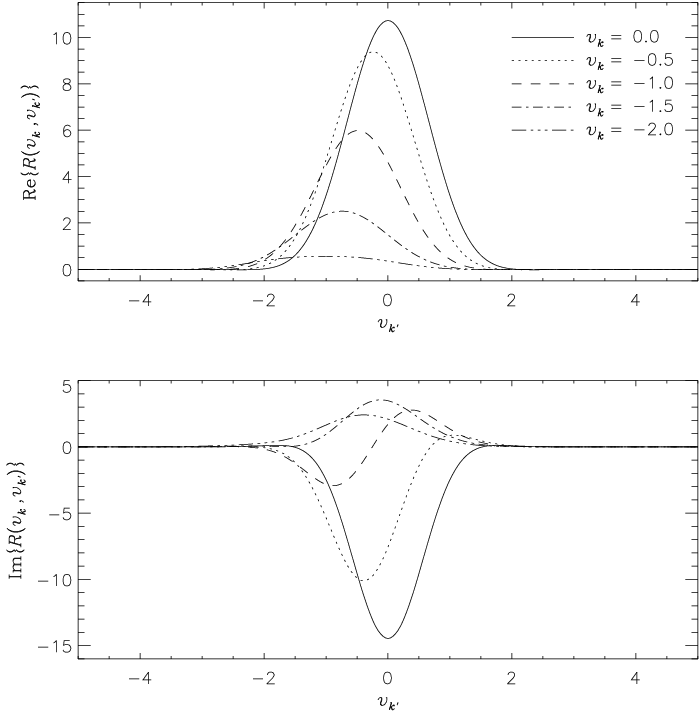
Figure 2.— The real (top) and imaginary (bottom) parts of the integral of the redistribution function of Equation (17) over the normalized output frequency vk′≡12​(wu​f+wu′​f)v_{k^{\prime}}\equiv\frac{1}{2}(w_{uf}+w_{u^{\prime}f}), plotted against the normalized input frequency vk≡12​(vu​l+vu′​l′)v_{k}\equiv\frac{1}{2}(v_{ul}+v_{u^{\prime}l^{\prime}}). The different curves correspond to different values of the ratio vl​l′≡ωl​l′/Δv_{ll^{\prime}}\equiv\omega_{ll^{\prime}}/\Delta. For this example, we assumed a scattering angle Θ=\Theta=1 rad, and a fully degenerate upper level (i.e., ωu​u′=0\omega_{uu^{\prime}}=0).

Owing to the fact that |F′​(x)|≤1|F^{\prime}(x)|\leq 1 over the real domain [1, e.g.,], from the mean-value theorem it follows that

|F⁡(vu​l′−wu​f+p⁡(1−C​ξl/ξf)S​ξl)−F⁡(vu​l−wu​f+p⁡(1−C​ξl/ξf)S​ξl)|≤|ωl​l′|Δ​S​ξl.\left|F\biggl(\frac{v_{ul^{\prime}}-w_{uf}+p(1-C\xi_{l}/\xi_{f})}{S\xi_{l}}\biggr)-F\biggl(\frac{v_{ul}-w_{uf}+p(1-C\xi_{l}/\xi_{f})}{S\xi_{l}}\biggr)\right|\leq\frac{|\omega_{ll^{\prime}}|}{\Delta S\xi_{l}}\;.

This allows us to estimate a bound to the integral contribution of Equation (17). In fact,

1π∫−∞+∞dpe−p2/ξf2|1au+i⁡(p−wu​f)+1au′−i⁡(p−wu′​f)|\displaystyle\frac{1}{\pi}\int_{-\infty}^{+\infty}dp\;{\rm e}^{-p^{2}/\xi_{f}^{2}}\biggl|\frac{1}{a_{u}+{\rm i}(p-w_{uf})}+\frac{1}{a_{u^{\prime}}-{\rm i}(p-w_{u^{\prime}f})}\biggr| (18)
≤\displaystyle\leq H(wu​fξf,auξf)+H(wu′​fξf,au′ξf)+1π∫−∞+∞dpe−p2/ξf2[|p−wu​f|au2+(p−wu​f)2+|p−wu′​f|au′2+(p−wu′​f)2]\displaystyle H\!\left(\frac{w_{uf}}{\xi_{f}},\frac{a_{u}}{\xi_{f}}\right)+H\!\left(\frac{w_{u^{\prime}f}}{\xi_{f}},\frac{a_{u^{\prime}}}{\xi_{f}}\right)+\frac{1}{\pi}\int_{-\infty}^{+\infty}dp\;{\rm e}^{-p^{2}/\xi_{f}^{2}}\biggl[\frac{|p-w_{uf}|}{a_{u}^{2}+(p-w_{uf})^{2}}+\frac{|p-w_{u^{\prime}f}|}{a_{u^{\prime}}^{2}+(p-w_{u^{\prime}f})^{2}}\biggr]
≤\displaystyle\leq H(wu​fξf,auξf)+H(wu′​fξf,au′ξf)+12​π∫−∞+∞dpe−p2/ξf2(1au+1au′)\displaystyle H\!\left(\frac{w_{uf}}{\xi_{f}},\frac{a_{u}}{\xi_{f}}\right)+H\!\left(\frac{w_{u^{\prime}f}}{\xi_{f}},\frac{a_{u^{\prime}}}{\xi_{f}}\right)+\frac{1}{2\pi}\int_{-\infty}^{+\infty}dp\;{\rm e}^{-p^{2}/\xi_{f}^{2}}\biggl(\frac{1}{a_{u}}+\frac{1}{a_{u^{\prime}}}\biggr)
=\displaystyle= H⁡(wu​fξf,auξf)+H⁡(wu′​fξf,au′ξf)+ξf2​π​(1au+1au′),\displaystyle H\!\left(\frac{w_{uf}}{\xi_{f}},\frac{a_{u}}{\xi_{f}}\right)+H\!\left(\frac{w_{u^{\prime}f}}{\xi_{f}},\frac{a_{u^{\prime}}}{\xi_{f}}\right)+\frac{\xi_{f}}{2\sqrt{\pi}}\biggl(\frac{1}{a_{u}}+\frac{1}{a_{u^{\prime}}}\biggr)\;,

and so the integral contribution in Equation (17) can be neglected when the quantity

2π​|ωl​l′|Δ​S​ξl​[H⁡(wu​fξf,auξf)+H⁡(wu′​fξf,au′ξf)+ξf2​π​(1au+1au′)]\frac{2}{\sqrt{\pi}}\,\frac{|\omega_{ll^{\prime}}|}{\Delta S\xi_{l}}\,\biggl[H\!\left(\frac{w_{uf}}{\xi_{f}},\frac{a_{u}}{\xi_{f}}\right)+H\!\left(\frac{w_{u^{\prime}f}}{\xi_{f}},\frac{a_{u^{\prime}}}{\xi_{f}}\right)+\frac{\xi_{f}}{2\sqrt{\pi}}\biggl(\frac{1}{a_{u}}+\frac{1}{a_{u^{\prime}}}\biggr)\biggr]

is sufficiently small compared to the absolute value of the contribution within curly brackets in that same equation.

Refer to caption
Figure 3.— The real (top) and imaginary (bottom) parts of the redistribution function of Equation (17) plotted against the normalized output frequency vk′≡12​(wu​f+wu′​f)v_{k^{\prime}}\equiv\frac{1}{2}(w_{uf}+w_{u^{\prime}f}), for various values of the normalized input frequency vk≡12​(vu​l+vu′​l′)v_{k}\equiv\frac{1}{2}(v_{ul}+v_{u^{\prime}l^{\prime}}). For this example, we assumed ωl​l′=0.5​Δ\omega_{ll^{\prime}}=0.5\,\Delta and ωu​u′=0.2​Δ\omega_{uu^{\prime}}=0.2\,\Delta.

Figure 2 shows the integral over the normalized output frequency vk′≡12​(wu​f+wu′​f)v_{k^{\prime}}\equiv\frac{1}{2}(w_{uf}+w_{u^{\prime}f}) of the redistribution function of Equation (17), plotted against the normalized input frequency vk≡12​(vu​l+vu′​l′)v_{k}\equiv\frac{1}{2}(v_{ul}+v_{u^{\prime}l^{\prime}}). The upper (lower) panel shows the real (imaginary) part of this integral. The different curves correspond to different values of the quantity vl​l′≡ωl​l′/Δv_{ll^{\prime}}\equiv\omega_{ll^{\prime}}/\Delta. For this example, we assumed a scattering angle Θ=1\Theta=1 rad, and a fully degenerate upper state, so that ωu​u′=0\omega_{uu^{\prime}}=0. In such a case, we see from Equation (17) that the contribution within curly brackets is purely real. Therefore, the plots in the lower panel are exclusively due to the integral term in Equation (17). We can conclude from those plots that the contribution of the integral term is generally not negligible, so it can significantly affect the shape of the redistributed profile depending on the importance of the lower-term coherence. In contrast, the integral term brings no contribution when the atom is illuminated with a flat spectrum, owing to the fact that its integral over vkv_{k} vanishes identically (see Figure 2, and the comment at the end of Appendix C).

In the particular case when the atomic coherence of the lower term is completely relaxed (ρl​l′=δl​l′​ρl​l\rho_{ll^{\prime}}=\delta_{ll^{\prime}}\,\rho_{ll}), or if the levels ll and l′l^{\prime} are completely degenerate, the integral contribution vanishes, and Equation (17) provides the generalization of the well-known RIIR_{\rm II} redistribution function [10, e.g.,] to the case of a Λ\Lambda-type three-term atom,

RII​(Ωu,Ωu′,Ωl,Ωf,ω^k,ω^k′,Θ)\displaystyle R_{\rm II}(\Omega_{u},\Omega_{u^{\prime}};\Omega_{l},\Omega_{f};\hat{\omega}_{k},\hat{\omega}_{k^{\prime}};\Theta) =\displaystyle= 2​πΔ2​S​ξl​ξf​exp⁡[−(ω^k−ω^k′+ωl​f)2Δ2]\displaystyle\frac{2\pi}{\Delta^{2}\,S\xi_{l}\xi_{f}}\,\exp\biggl[-\frac{(\hat{\omega}_{k}-\hat{\omega}_{k^{\prime}}+\omega_{lf})^{2}}{\Delta^{2}}\biggr] (19)
×[W⁡(κ+​vu​l+κ−​wu​fS​ξl​ξf,auS​ξl​ξf)+W¯​(κ+​vu′​l+κ−​wu′​fS​ξl​ξf,au′S​ξl​ξf)].\displaystyle\kern-85.35826pt{}\times\biggl[W\biggl(\frac{\kappa^{+}v_{ul}+\kappa^{-}w_{uf}}{S\xi_{l}\xi_{f}},\frac{a_{u}}{S\xi_{l}\xi_{f}}\biggr)+\overline{W}\biggl(\frac{\kappa^{+}v_{u^{\prime}l}+\kappa^{-}w_{u^{\prime}f}}{S\xi_{l}\xi_{f}},\frac{a_{u^{\prime}}}{S\xi_{l}\xi_{f}}\biggr)\biggr]\;.

This expression was applied in recent work that investigated the effects of partial redistribution on the formation of polarized lines from Λ\Lambda-type three-term atoms in the solar spectrum [3].

Finally, Figure 3 shows several realizations of the full redistribution function of Equation (17) plotted against the normalized output frequency vk′v_{k^{\prime}}, for different values of the normalized input frequency vkv_{k}. For the example in this figure, we assumed ωl​l′=0.5​Δ\omega_{ll^{\prime}}=0.5\,\Delta and ωu​u′=0.2​Δ\omega_{uu^{\prime}}=0.2\,\Delta, and a scattering angle Θ=1\Theta=1 rad.

IV. The cases of forward and backward scattering

In the two cases of forward and backward scattering (Θ=0\Theta=0 and Θ=π\Theta=\pi, respectively), the expression (17) for the laboratory redistribution function breaks down because of the condition S=0S=0. We can, however, treat these two cases relying on a physical argument of continuity, and taking the limit of the redistribution function for S→0+S\to 0^{+}. Using the asymptotic expansion of W⁡(v,a)W(v,a) for large values of |v+i​a||v+{\rm i}a| [7, e.g.,], and recalling Equation (B3), it can be shown that

limk→0+1k​W​(vk,ak)=iπ​(v+i​a),limk→0+1k​F​(vk)=12​v.\lim_{k\to 0^{+}}\frac{1}{k}\,W\Bigl(\frac{v}{k},\frac{a}{k}\Bigr)=\frac{{\rm i}}{\sqrt{\pi}\,(v+{\rm i}a)}\;,\qquad\lim_{k\to 0^{+}}\frac{1}{k}\,F\Bigl(\frac{v}{k}\Bigr)=\frac{1}{2v}\;. (20)

Considering for simplicity the case of non-coherent lower term, Equation (19) thus becomes, for the two cases of forward and backward scattering,

RII​(Ωu,Ωu′,Ωl,Ωf,ω^k,ω^k′,C=±1)\displaystyle R_{\rm II}(\Omega_{u},\Omega_{u^{\prime}};\Omega_{l},\Omega_{f};\hat{\omega}_{k},\hat{\omega}_{k^{\prime}};C=\pm 1) =\displaystyle= 2​πΔ∓​exp⁡[−(ω^k−ω^k′+ωl​f)2Δ∓2]\displaystyle\frac{2\sqrt{\pi}}{\Delta_{\mp}}\,\exp\biggl[-\frac{(\hat{\omega}_{k}-\hat{\omega}_{k^{\prime}}+\omega_{lf})^{2}}{\Delta_{\mp}^{2}}\biggr] (21)
×[iκ+​(ω^k−ωu​l)+κ−​(ω^k′−ωu​f)+i​ϵu−iκ+​(ω^k−ωu′​l)+κ−​(ω^k′−ωu′​f)−i​ϵu′],\displaystyle\kern-180.67499pt{}\times\biggl[\frac{{\rm i}}{\kappa^{+}(\hat{\omega}_{k}-\omega_{ul})+\kappa^{-}(\hat{\omega}_{k^{\prime}}-\omega_{uf})+{\rm i}\epsilon_{u}}-\frac{{\rm i}}{\kappa^{+}(\hat{\omega}_{k}-\omega_{u^{\prime}l})+\kappa^{-}(\hat{\omega}_{k^{\prime}}-\omega_{u^{\prime}f})-{\rm i}\epsilon_{u^{\prime}}}\biggr]\;,

where Δ±=Δu​l±Δu​f\Delta_{\pm}=\Delta_{ul}\pm\Delta_{uf}.

Refer to caption
Figure 4.— Plots showing the transition between the forms (19) and (21) of RIIR_{\rm II} in approaching the condition of forward scattering. The atomic model adopted is that of the three-term Ca II ion encompassing the formation of the H and K lines and the IR triplet. The plots show the Raman scattered emissivity in the polarized Ca II K line due to the monochromatic excitation of the Ca II 854.2 nm line at the exact value of its resonance frequency, and for different values of the scattering angle Θ\Theta near 0∘0^{\circ}.

IV.1. The Special Case of the Two-term Atom

When the two lower terms coincide, so that Δu​f=Δu​l\Delta_{uf}=\Delta_{ul}, the asymptotic result expressed by Equation (20) is not generally applicable. In fact, in the case of a two-term atom with non-coherent lower term, Equation (19) becomes

RII​(Ωu,Ωu′,Ωl,Ωf,ω^k,ω^k′,Θ)\displaystyle R_{\rm II}(\Omega_{u},\Omega_{u^{\prime}};\Omega_{l},\Omega_{f};\hat{\omega}_{k},\hat{\omega}_{k^{\prime}};\Theta) =\displaystyle= πΔ​ωT2​C2​S2​exp⁡[−(ω^k−ω^k′+ωl​f)24​S22​Δ​ωT2]\displaystyle\frac{\pi}{\Delta\omega_{T}^{2}\,C_{2}S_{2}}\exp\!\left[-\frac{(\hat{\omega}_{k}-\hat{\omega}_{k^{\prime}}+\omega_{lf})^{2}}{4S_{2}^{2}\Delta\omega_{T}^{2}}\right] (22)
×[W⁡(ω^k+ω^k′−ωu​l−ωu​f2​C2​Δ​ωT,ϵuC2​Δ​ωT)+W¯​(ω^k+ω^k′−ωu′​l−ωu′​f2​C2​Δ​ωT,ϵu′C2​Δ​ωT)],\displaystyle\kern-144.54pt{}\times\left[W\biggl(\frac{\hat{\omega}_{k}+\hat{\omega}_{k^{\prime}}-\omega_{ul}-\omega_{uf}}{2C_{2}\Delta\omega_{T}},\frac{\epsilon_{u}}{C_{2}\Delta\omega_{T}}\biggr)+\overline{W}\biggl(\frac{\hat{\omega}_{k}+\hat{\omega}_{k^{\prime}}-\omega_{u^{\prime}l}-\omega_{u^{\prime}f}}{2C_{2}\Delta\omega_{T}},\frac{\epsilon_{u^{\prime}}}{C_{2}\Delta\omega_{T}}\biggr)\right]\;,

where we indicated with Δ​ωT=Δu​l=Δu​f\Delta\omega_{T}=\Delta_{ul}=\Delta_{uf} the single value of the Doppler width of the two-term transition, and we also defined S2=sin⁡(Θ/2)S_{2}=\sin(\Theta/2) and C2=cos⁡(Θ/2)C_{2}=\cos(\Theta/2) (cf. Paper I). Then the limit (20) applies only to the case of backward scattering (C2→0)(C_{2}\to 0), but not to forward scattering (S2→0)(S_{2}\to 0). In the first case, we obtain an expression formally identical to Equation (21), namely,

RII​(Ωu,Ωu′,Ωl,Ωf,ω^k,ω^k′,Θ=π)\displaystyle R_{\rm II}(\Omega_{u},\Omega_{u^{\prime}};\Omega_{l},\Omega_{f};\hat{\omega}_{k},\hat{\omega}_{k^{\prime}};\Theta=\pi) =\displaystyle= 2​πΔ​ωT​exp⁡[−(ω^k−ω^k′+ωl​f)24​Δ​ωT2]\displaystyle\frac{2\sqrt{\pi}}{\Delta\omega_{T}}\,\exp\biggl[-\frac{(\hat{\omega}_{k}-\hat{\omega}_{k^{\prime}}+\omega_{lf})^{2}}{4\Delta\omega_{T}^{2}}\biggr] (23)
×(iω^k+ω^k′−ωu​l−ωu​f+2​i​ϵu−iω^k+ω^k′−ωu′​l−ωu′​f−2​i​ϵu′),\displaystyle\kern-144.54pt{}\times\Biggl(\frac{{\rm i}}{\hat{\omega}_{k}+\hat{\omega}_{k^{\prime}}-\omega_{ul}-\omega_{uf}+2{\rm i}\epsilon_{u}}-\frac{{\rm i}}{\hat{\omega}_{k}+\hat{\omega}_{k^{\prime}}-\omega_{u^{\prime}l}-\omega_{u^{\prime}f}-2{\rm i}\epsilon_{u^{\prime}}}\Biggr)\;,

whereas in the case of forward scattering,

RII​(Ωu,Ωu′,Ωl,Ωf,ω^k,ω^k′,Θ=0)\displaystyle R_{\rm II}(\Omega_{u},\Omega_{u^{\prime}};\Omega_{l},\Omega_{f};\hat{\omega}_{k},\hat{\omega}_{k^{\prime}};\Theta=0) =\displaystyle= 2​π​πΔ​ωT​δ​(ω^k−ω^k′+ωl​f)\displaystyle\frac{2\pi\sqrt{\pi}}{\Delta\omega_{T}}\,\delta(\hat{\omega}_{k}-\hat{\omega}_{k^{\prime}}+\omega_{lf}) (24)
×[W⁡(ω^k′−ωu​fΔ​ωT,ϵuΔ​ωT)+W¯​(ω^k′−ωu′​fΔ​ωT,ϵu′Δ​ωT)],\displaystyle\kern-108.405pt{}\times\left[W\biggl(\frac{\hat{\omega}_{k^{\prime}}-\omega_{uf}}{\Delta\omega_{T}},\frac{\epsilon_{u}}{\Delta\omega_{T}}\biggr)+\overline{W}\biggl(\frac{\hat{\omega}_{k^{\prime}}-\omega_{u^{\prime}f}}{\Delta\omega_{T}},\frac{\epsilon_{u^{\prime}}}{\Delta\omega_{T}}\biggr)\right]\;,

owing to the fact that exp(−x2/k2)/k→πδ(x)\exp(-x^{2}/k^{2})/k\to\sqrt{\pi}\,\delta(x) when k→0+k\to 0^{+}. This last expression in particular shows that the process of forward scattering in a two-term atom is strictly coherent. In fact, from a simple inspection of Equation (21) it is already possible to conclude that both processes of forward and backward scattering imply an increased degree of correlation between the input and output frequencies [cf. 8, and references therein], with a typical spread that is dominated by the inverse lifetime of the upper level, rather than by the Doppler width. However, only in the case of forward scattering in a two-term atom, strict coherence is attained, according to Equation (24).

The plots in Figure 4 show an example of the behavior of the scattered polarized emissivity in a three-term atomic system when the scattering angle approaches 0∘0^{\circ}. For the example in this figure, we adopted the three-term model of the Ca II ion underlying the formation of the H and K doublet around 395 nm and the IR triplet around 858 nm. The line formation model also includes a magnetic field of 10 G normal to the direction of the incident light, which is responsible for the appearance of line polarization, and in particular of non-vanishing Stokes UU and VV signals when the scattering direction forms an angle with the incidence direction. The plotted profiles of the Ca II K line at 393.4 nm are produced by Raman scattering of monochromatic radiation at the exact resonance frequency of the 854.2 nm line of the IR triplet. For the modeling we assumed a plasma density of 1012​cm−310^{12}\,\rm cm^{-3} and a temperature of 1000 K, which corresponds to a Doppler width of 8.5 mÅ. However, because of the near condition of forward scattering, the actual width of the scattered profiles is instead dominated by the natural linewidth (∼0.5\sim 0.5 mÅ), as expected. Figure 4 numerically demonstrates how Equation (21) indeed provides the correct limit of the general expression (19) of RIIR_{\rm II}, when approaching the condition of forward scattering, as both Stokes II and QQ for Θ=0.1∘\Theta=0.1^{\circ} are already practically indistinguishable from those at Θ=0∘\Theta=0^{\circ}.

We thank T. del Pino Alemán (HAO) for internally reviewing the manuscript and for helpful comments. We are deeply indebted to the anonymous referee, for a very careful review of our manuscript and for helpful comments and suggestions that have greatly improved the presentation of this work.

Appendix A Formal limit for the condition of metastable initial and final terms

In order to derive the form of Equation (11) for the case of metastable initial and final states, we must consider two possibilities in taking the limit for a¯l,l′,f→0\bar{a}_{l,l^{\prime},f}\to 0, which correspond to the assumptions that a¯f≷a¯l,l′\bar{a}_{f}\gtrless\bar{a}_{l,l^{\prime}}. We then find, in that limit,

R​(Ωu,Ωu′,Ωl,Ωl′,Ωf,ω^k,ω^k′,Θ)s.l.l.\displaystyle R(\Omega_{u},\Omega_{u^{\prime}};\Omega_{l},\Omega_{l^{\prime}},\Omega_{f};\hat{\omega}_{k},\hat{\omega}_{k^{\prime}};\Theta)_{\rm s.l.l.} =\displaystyle= 1Δ2​S​ξl​ξf​∫−∞+∞d​q¯​e−S2​ξl2​ξf2​q¯2\displaystyle\frac{1}{\Delta^{2}\,S\xi_{l}\xi_{f}}\int_{-\infty}^{+\infty}d\bar{q}\;{\rm e}^{-S^{2}\xi_{l}^{2}\xi_{f}^{2}\bar{q}^{2}} (A1)
×{W(xu​l′,a¯u)[πδ(xu​l′−yu​f)+iPv1xu​l′−yu​f]+W¯(xu′​l,a¯u′)[πδ(xu′​l−yu′​f)−iPv1xu′​l−yu′​f]\displaystyle\kern-180.67499pt\times\Biggl\{W\bigl(x_{ul^{\prime}},\bar{a}_{u}\bigr)\biggl[\pi\delta(x_{ul^{\prime}}-y_{uf})+{\rm i}\,{\rm Pv}\frac{1}{x_{ul^{\prime}}-y_{uf}}\biggr]+\overline{W}\bigl(x_{u^{\prime}l},\bar{a}_{u^{\prime}}\bigr)\biggl[\pi\delta(x_{u^{\prime}l}-y_{u^{\prime}f})-{\rm i}\,{\rm Pv}\frac{1}{x_{u^{\prime}l}-y_{u^{\prime}f}}\biggr]
+W⁡(yu​f,a¯u)​[π​δ​(xu​l−yu​f)−i​Pv​1xu​l−yu​f]+W¯​(yu′​f,a¯u′)​[π​δ​(xu′​l′−yu′​f)+i​Pv​1xu′​l′−yu′​f]\displaystyle\kern-180.67499pt\,\,{}+W\bigl(y_{uf},\bar{a}_{u}\bigr)\biggl[\pi\delta(x_{ul}-y_{uf})-{\rm i}\,{\rm Pv}\frac{1}{x_{ul}-y_{uf}}\biggr]+\overline{W}\bigl(y_{u^{\prime}f},\bar{a}_{u^{\prime}}\bigr)\biggl[\pi\delta(x_{u^{\prime}l^{\prime}}-y_{u^{\prime}f})+{\rm i}\,{\rm Pv}\frac{1}{x_{u^{\prime}l^{\prime}}-y_{u^{\prime}f}}\biggr]
+[W⁡(xu​l′,a¯u)−W⁡(yu​f,a¯u)]​[±π​δ​(xu​l′−yu​f)−i​Pv​1xu​l′−yu​f]\displaystyle\kern-180.67499pt\,\,{}+\Bigl[W\bigl(x_{ul^{\prime}},\bar{a}_{u}\bigr)-W\bigl(y_{uf},\bar{a}_{u}\bigr)\Bigr]\biggl[\pm\pi\delta(x_{ul^{\prime}}-y_{uf})-{\rm i}\,{\rm Pv}\frac{1}{x_{ul^{\prime}}-y_{uf}}\biggr]
+[W¯(xu′​l,a¯u′)−W¯(yu′​f,a¯u′)][±πδ(xu′​l−yu′​f)+iPv1xu′​l−yu′​f]},\displaystyle\kern-180.67499pt\,\,{}+\Bigl[\overline{W}\bigl(x_{u^{\prime}l},\bar{a}_{u^{\prime}}\bigr)-\overline{W}\bigl(y_{u^{\prime}f},\bar{a}_{u^{\prime}}\bigr)\Bigr]\biggl[\pm\pi\delta(x_{u^{\prime}l}-y_{u^{\prime}f})+{\rm i}\,{\rm Pv}\frac{1}{x_{u^{\prime}l}-y_{u^{\prime}f}}\biggr]\Biggr\}\;,

where the ±\pm sign in front of the Dirac-δ\deltas in the last two lines must be chosen according to whether a¯f≷a¯l\bar{a}_{f}\gtrless\bar{a}_{l}. By noting that

W⁡(yu​f,a¯u)​δ​(xu​l′−yu​f)\displaystyle W\bigl(y_{uf},\bar{a}_{u}\bigr)\,\delta(x_{ul^{\prime}}-y_{uf}) =\displaystyle= W⁡(xu​l′,a¯u)​δ​(xu​l′−yu​f),\displaystyle W\bigl(x_{ul^{\prime}},\bar{a}_{u}\bigr)\,\delta(x_{ul^{\prime}}-y_{uf})\;,
W¯​(yu′​f,a¯u′)​δ​(xu′​l−yu′​f)\displaystyle\overline{W}\bigl(y_{u^{\prime}f},\bar{a}_{u^{\prime}}\bigr)\,\delta(x_{u^{\prime}l}-y_{u^{\prime}f}) =\displaystyle= W¯​(xu′​l,a¯u′)​δ​(xu′​l−yu′​f),\displaystyle\overline{W}\bigl(x_{u^{\prime}l},\bar{a}_{u^{\prime}}\bigr)\,\delta(x_{u^{\prime}l}-y_{u^{\prime}f})\;,

we see that the terms carrying a sign choice vanish identically, and so we are left with

R​(Ωu,Ωu′,Ωl,Ωl′,Ωf,ω^k,ω^k′,Θ)s.l.l.\displaystyle R(\Omega_{u},\Omega_{u^{\prime}};\Omega_{l},\Omega_{l^{\prime}},\Omega_{f};\hat{\omega}_{k},\hat{\omega}_{k^{\prime}};\Theta)_{\rm s.l.l.} =\displaystyle= πΔ2​S​ξl​ξf​∫−∞+∞d​q¯​e−S2​ξl2​ξf2​q¯2\displaystyle\frac{\pi}{\Delta^{2}\,S\xi_{l}\xi_{f}}\int_{-\infty}^{+\infty}d\bar{q}\;{\rm e}^{-S^{2}\xi_{l}^{2}\xi_{f}^{2}\bar{q}^{2}} (A2)
×{W(xu​l′,a¯u)δ(xu​l′−yu​f)+W¯(xu′​l,a¯u′)δ(xu′​l−yu′​f)+W(yu​f,a¯u)δ(xu​l−yu​f)+W¯(yu′​f,a¯u′)δ(xu′​l′−yu′​f)\displaystyle\kern-158.99377pt\times\Biggl\{W\bigl(x_{ul^{\prime}},\bar{a}_{u}\bigr)\,\delta(x_{ul^{\prime}}-y_{uf})+\overline{W}\bigl(x_{u^{\prime}l},\bar{a}_{u^{\prime}}\bigr)\,\delta(x_{u^{\prime}l}-y_{u^{\prime}f})+W\bigl(y_{uf},\bar{a}_{u}\bigr)\,\delta(x_{ul}-y_{uf})+\overline{W}\bigl(y_{u^{\prime}f},\bar{a}_{u^{\prime}}\bigr)\,\delta(x_{u^{\prime}l^{\prime}}-y_{u^{\prime}f})
+iπW(yu​f,a¯u)(Pv1xu​l′−yu​f−Pv1xu​l−yu​f)+iπW¯(yu′​f,a¯u′)(Pv1xu′​l′−yu′​f−Pv1xu′​l−yu′​f)},\displaystyle\kern-158.99377pt\,\,{}+\frac{\rm i}{\pi}\,W\bigl(y_{uf},\bar{a}_{u}\bigr)\biggl({\rm Pv}\frac{1}{x_{ul^{\prime}}-y_{uf}}-{\rm Pv}\frac{1}{x_{ul}-y_{uf}}\biggr)+\frac{\rm i}{\pi}\,\overline{W}\bigl(y_{u^{\prime}f},\bar{a}_{u^{\prime}}\bigr)\biggl({\rm Pv}\frac{1}{x_{u^{\prime}l^{\prime}}-y_{u^{\prime}f}}-{\rm Pv}\frac{1}{x_{u^{\prime}l}-y_{u^{\prime}f}}\biggr)\Biggr\}\;,

We now substitute back the relations (9) and (10) that hold for the variables xa​bx_{ab} and ya​by_{ab}:

R​(Ωu,Ωu′,Ωl,Ωl′,Ωf,ω^k,ω^k′,Θ)s.l.l.\displaystyle R(\Omega_{u},\Omega_{u^{\prime}};\Omega_{l},\Omega_{l^{\prime}},\Omega_{f};\hat{\omega}_{k},\hat{\omega}_{k^{\prime}};\Theta)_{\rm s.l.l.} =\displaystyle= πΔ2​S​ξl​ξf​∫−∞+∞d​q¯​e−S2​ξl2​ξf2​q¯2\displaystyle\frac{\pi}{\Delta^{2}\,S\xi_{l}\xi_{f}}\int_{-\infty}^{+\infty}d\bar{q}\;{\rm e}^{-S^{2}\xi_{l}^{2}\xi_{f}^{2}\bar{q}^{2}} (A3)
×[W(v¯u​l′+q¯(Cξlξf−ξl2),a¯u)δ(v¯u​l′−w¯u​f−q¯)+W¯(v¯u′​l+q¯(Cξlξf−ξl2),a¯u′)δ(v¯u′​l−w¯u′​f−q¯)\displaystyle\kern-158.99377pt\times\Bigr[\,W\bigl(\bar{v}_{ul^{\prime}}+\bar{q}(C\xi_{l}\xi_{f}-\xi_{l}^{2}),\bar{a}_{u}\bigr)\,\delta(\bar{v}_{ul^{\prime}}-\bar{w}_{uf}-\bar{q}\bigr)+\overline{W}\bigl(\bar{v}_{u^{\prime}l}+\bar{q}(C\xi_{l}\xi_{f}-\xi_{l}^{2}),\bar{a}_{u^{\prime}}\bigr)\,\delta(\bar{v}_{u^{\prime}l}-\bar{w}_{u^{\prime}f}-\bar{q}\bigr)
+W(w¯u​f+q¯(ξf2−Cξlξf),a¯u)δ(v¯u​l−w¯u​f−q¯)+W¯(w¯u′​f+q¯(ξf2−Cξlξf),a¯u′)δ(v¯u′​l′−w¯u′​f−q¯)]\displaystyle\kern-158.99377pt\,{}+W\bigl(\bar{w}_{uf}+\bar{q}(\xi_{f}^{2}-C\xi_{l}\xi_{f}),\bar{a}_{u}\bigr)\,\delta(\bar{v}_{ul}-\bar{w}_{uf}-\bar{q}\bigr)+\overline{W}\bigl(\bar{w}_{u^{\prime}f}+\bar{q}(\xi_{f}^{2}-C\xi_{l}\xi_{f}),\bar{a}_{u^{\prime}}\bigr)\,\delta(\bar{v}_{u^{\prime}l^{\prime}}-\bar{w}_{u^{\prime}f}-\bar{q}\bigr)\Bigr]
+iΔ2​S​ξl​ξf∫−∞+∞dq¯e−S2​ξl2​ξf2​q¯2{W(w¯u​f+q¯(ξf2−Cξlξf),a¯u)(Pv1v¯u​l′−w¯u​f−q¯−Pv1v¯u​l−w¯u​f−q¯)\displaystyle\kern-169.83493pt{}+\frac{\rm i}{\Delta^{2}\,S\xi_{l}\xi_{f}}\int_{-\infty}^{+\infty}d\bar{q}\;{\rm e}^{-S^{2}\xi_{l}^{2}\xi_{f}^{2}\bar{q}^{2}}\Biggl\{W\bigl(\bar{w}_{uf}+\bar{q}(\xi_{f}^{2}-C\xi_{l}\xi_{f}),\bar{a}_{u}\bigr)\biggl({\rm Pv}\frac{1}{\bar{v}_{ul^{\prime}}-\bar{w}_{uf}-\bar{q}}-{\rm Pv}\frac{1}{\bar{v}_{ul}-\bar{w}_{uf}-\bar{q}}\biggr)
+W¯(w¯u′​f+q¯(ξf2−Cξlξf),a¯u′)(Pv1v¯u′​l′−w¯u′​f−q¯−Pv1v¯u′​l−w¯u′​f−q¯)}\displaystyle\kern-25.29494pt{}+\overline{W}\bigl(\bar{w}_{u^{\prime}f}+\bar{q}(\xi_{f}^{2}-C\xi_{l}\xi_{f}),\bar{a}_{u^{\prime}}\bigr)\biggl({\rm Pv}\frac{1}{\bar{v}_{u^{\prime}l^{\prime}}-\bar{w}_{u^{\prime}f}-\bar{q}}-{\rm Pv}\frac{1}{\bar{v}_{u^{\prime}l}-\bar{w}_{u^{\prime}f}-\bar{q}}\biggr)\Biggr\}
≡πΔ2​S​ξl​ξf{W(κ+​vu​l′+κ−​wu​fS​ξl​ξf,auS​ξl​ξf)exp[−(vu​l′−wu​f)2]+W¯(κ+​vu′​l+κ−​wu′​fS​ξl​ξf,au′S​ξl​ξf)exp[−(vu′​l−wu′​f)2]\displaystyle\kern-169.83493pt\,\mathop{\equiv}\frac{\pi}{\Delta^{2}\,S\xi_{l}\xi_{f}}\Biggl\{W\biggl(\frac{\kappa^{+}v_{ul^{\prime}}+\kappa^{-}w_{uf}}{S\xi_{l}\xi_{f}},\frac{a_{u}}{S\xi_{l}\xi_{f}}\biggr)\,\exp\!\left[-(v_{ul^{\prime}}-w_{uf})^{2}\right]+\overline{W}\biggl(\frac{\kappa^{+}v_{u^{\prime}l}+\kappa^{-}w_{u^{\prime}f}}{S\xi_{l}\xi_{f}},\frac{a_{u^{\prime}}}{S\xi_{l}\xi_{f}}\biggr)\,\exp\!\left[-(v_{u^{\prime}l}-w_{u^{\prime}f})^{2}\right]
+W(κ+​vu​l+κ−​wu​fS​ξl​ξf,auS​ξl​ξf)exp[−(vu​l−wu​f)2]+W¯(κ+​vu′​l′+κ−​wu′​fS​ξl​ξf,au′S​ξl​ξf)exp[−(vu′​l′−wu′​f)2]}\displaystyle\kern-133.69994pt{}+W\biggl(\frac{\kappa^{+}v_{ul}+\kappa^{-}w_{uf}}{S\xi_{l}\xi_{f}},\frac{a_{u}}{S\xi_{l}\xi_{f}}\biggr)\,\exp\!\left[-(v_{ul}-w_{uf})^{2}\right]+\overline{W}\biggl(\frac{\kappa^{+}v_{u^{\prime}l^{\prime}}+\kappa^{-}w_{u^{\prime}f}}{S\xi_{l}\xi_{f}},\frac{a_{u^{\prime}}}{S\xi_{l}\xi_{f}}\biggr)\,\exp\!\left[-(v_{u^{\prime}l^{\prime}}-w_{u^{\prime}f})^{2}\right]\Biggr\}
+iΔ2​S​ξl​ξf−∫−∞+∞dqe−q2{W(wu​f+q⁡(ξf2−C​ξl​ξf)S​ξl​ξf,auS​ξl​ξf)(1vu​l′−wu​f−q−1vu​l−wu​f−q)\displaystyle\kern-169.83493pt\,\mathop{+}\frac{\rm i}{\Delta^{2}\,S\xi_{l}\xi_{f}}\;{-}\kern-10.70009pt\intop\nolimits_{-\infty}^{+\infty}dq\;{\rm e}^{-q^{2}}\Biggl\{W\biggl(\frac{w_{uf}+q(\xi_{f}^{2}-C\xi_{l}\xi_{f})}{S\xi_{l}\xi_{f}},\frac{a_{u}}{S\xi_{l}\xi_{f}}\biggr)\biggl(\frac{1}{v_{ul^{\prime}}-w_{uf}-q}-\frac{1}{v_{ul}-w_{uf}-q}\biggr)
+W¯(wu′​f+q⁡(ξf2−C​ξl​ξf)S​ξl​ξf,au′S​ξl​ξf)(1vu′​l′−wu′​f−q−1vu′​l−wu′​f−q)},\displaystyle\kern-72.26999pt\,\,{}+\overline{W}\biggl(\frac{w_{u^{\prime}f}+q(\xi_{f}^{2}-C\xi_{l}\xi_{f})}{S\xi_{l}\xi_{f}},\frac{a_{u^{\prime}}}{S\xi_{l}\xi_{f}}\biggr)\biggl(\frac{1}{v_{u^{\prime}l^{\prime}}-w_{u^{\prime}f}-q}-\frac{1}{v_{u^{\prime}l}-w_{u^{\prime}f}-q}\biggr)\Biggr\}\;,

where we introduced new quantities (cf. Equation (4))

κ±=12​[1±(ξf2−ξl2)],\kappa^{\pm}={\textstyle\frac{1}{2}}\bigl[1\pm(\xi_{f}^{2}-\xi_{l}^{2})\bigr]\;, (A4)

and where the symbol −⁣∫{-}\kern-8.99994pt\intop in the last part indicates that the integral is taken in the principal value sense.

Finally, by recalling the definition (6) for the quantities va​bv_{ab} and wa​bw_{ab}, after reordering of some terms, we arrive at Equation (14).

Appendix B Transformation of the integral term

We consider the expression

𝒯=−∫−∞+∞dqe−q2W⁡((w+β​q)/N,a/N)v−w−q,{\cal T}=\;{-}\kern-10.70009pt\intop\nolimits_{-\infty}^{+\infty}dq\;{\rm e}^{-q^{2}}\,\frac{W((w+\beta q)/N,a/N)}{v-w-q}\;, (B1)

with N≡S​ξl​ξfN\equiv S\xi_{l}\xi_{f} and β≡ξf2−C​ξl​ξf\beta\equiv\xi_{f}^{2}-C\xi_{l}\xi_{f}. This expression provides the generic form of the various contributions to the integral term of Equation (14). Using the explicit form of W⁡(v,a)W(v,a), Equation (5), we find

𝒯\displaystyle{\cal T} =\displaystyle= 1π−∫−∞+∞d​q​∫−∞+∞d​p​e−p2a/N+i⁡[p−(w+β​q)/N]​e−q2v−w−q\displaystyle\frac{1}{\pi}\;{-}\kern-10.70009pt\intop\nolimits_{-\infty}^{+\infty}dq\int_{-\infty}^{+\infty}dp\;\frac{{\rm e}^{-p^{2}}}{a/N+{\rm i}[p-(w+\beta q)/N]}\,\frac{{\rm e}^{-q^{2}}}{v-w-q}
=\displaystyle= 1π−∫−∞+∞d​q​∫−∞+∞d​p​e−(p+β​q/N)2a/N+i⁡(p−w/N)​e−q2v−w−q,\displaystyle\frac{1}{\pi}\;{-}\kern-10.70009pt\intop\nolimits_{-\infty}^{+\infty}dq\int_{-\infty}^{+\infty}dp\;\frac{{\rm e}^{-(p+\beta q/N)^{2}}}{a/N+{\rm i}(p-w/N)}\,\frac{{\rm e}^{-q^{2}}}{v-w-q}\;,

where in the second line we operated the substitution p→p+β​q/Np\to p+\beta q/N. We note that

(p+β​qN)2+q2\displaystyle\biggl(p+\frac{\beta q}{N}\biggr)^{2}+q^{2} =\displaystyle= p2+2​βN​p​q+(1+β2N2)​q2≡p2+2​βN​p​q+q2α2\displaystyle p^{2}+2\frac{\beta}{N}\,pq+\biggl(1+\frac{\beta^{2}}{N^{2}}\biggr)q^{2}\equiv p^{2}+2\frac{\beta}{N}\,pq+\frac{q^{2}}{\alpha^{2}}
=\displaystyle= (1−α2​β2N2)​p2+(α​βN​p+qα)2=α2​p2+(α​βN​p+qα)2,\displaystyle\biggl(1-\frac{\alpha^{2}\beta^{2}}{N^{2}}\biggr)p^{2}+\biggl(\frac{\alpha\beta}{N}\,p+\frac{q}{\alpha}\biggr)^{2}=\alpha^{2}p^{2}+\biggl(\frac{\alpha\beta}{N}\,p+\frac{q}{\alpha}\biggr)^{2}\;,

where we put α2≡(1+β2/N2)−1=S2​ξl2\alpha^{2}\equiv(1+\beta^{2}/N^{2})^{-1}=S^{2}\xi_{l}^{2} (see Equation (4)). Defining next q~=q/α\tilde{q}=q/\alpha, we find at last

𝒯\displaystyle{\cal T} =\displaystyle= 1π​∫−∞+∞d​p​e−α2​p2a/N+i⁡(p−w/N)−∫−∞+∞d​q~​e−(q~+α​β​p/N)2(v−w)/α+α​β​p/N−(q~+α​β​p/N)\displaystyle\frac{1}{\pi}\int_{-\infty}^{+\infty}dp\;\frac{{\rm e}^{-\alpha^{2}p^{2}}}{a/N+{\rm i}(p-w/N)}\;{-}\kern-10.70009pt\intop\nolimits_{-\infty}^{+\infty}d\tilde{q}\;\frac{{\rm e}^{-(\tilde{q}+\alpha\beta p/N)^{2}}}{(v-w)/\alpha+\alpha\beta p/N-(\tilde{q}+\alpha\beta p/N)} (B2)
≡\displaystyle\equiv 2π​∫−∞+∞d​p​e−α2​p2a/N+i⁡(p−w/N)​F​(v−wα+α​βN​p)\displaystyle\frac{2}{\sqrt{\pi}}\int_{-\infty}^{+\infty}dp\;\frac{{\rm e}^{-\alpha^{2}p^{2}}}{a/N+{\rm i}(p-w/N)}\,F\biggl(\frac{v-w}{\alpha}+\frac{\alpha\beta}{N}\,p\biggr)
=\displaystyle= 2π​∫−∞+∞d​p​e−(α/N)2​p2a+i⁡(p−w)​F​(v−wα+α​βN2​p)\displaystyle\frac{2}{\sqrt{\pi}}\int_{-\infty}^{+\infty}dp\;\frac{{\rm e}^{-(\alpha/N)^{2}p^{2}}}{a+{\rm i}(p-w)}\,F\biggl(\frac{v-w}{\alpha}+\frac{\alpha\beta}{N^{2}}\,p\biggr)
=\displaystyle= 2π​∫−∞+∞d​p​e−p2/ξf2a+i⁡(p−w)​F​(v−w+p⁡(1−C​ξl/ξf)S​ξl),\displaystyle\frac{2}{\sqrt{\pi}}\int_{-\infty}^{+\infty}dp\;\frac{{\rm e}^{-p^{2}/\xi_{f}^{2}}}{a+{\rm i}(p-w)}\,F\biggl(\frac{v-w+p(1-C\xi_{l}/\xi_{f})}{S\xi_{l}}\biggr)\;,

where in the second line we recognized the integral over q~\tilde{q} to be the Hilbert transform of a Gaussian, which can therefore be expressed in terms of the Dawson’s integral function F⁡(x)F(x) [5, e.g.,].

Finally, we observe that

F⁡(v)=π2​L​(v,0),F(v)=\frac{\sqrt{\pi}}{2}\,L(v,0)\;, (B3)

where L⁡(v,a)L(v,a) is the imaginary part of the generalized Voigt function W⁡(v,a)W(v,a) of Equation (5). Hence the expression (B2) can conveniently be evaluated using the same algorithm adopted for the computation of W⁡(v,a)W(v,a).

Appendix C Normalization of the redistribution function

It is important to verify that the transformation of the redistribution function from the atomic frame of rest to the laboratory system preserves its norm, which also increases confidence in the correctness of the transformation itself. In order to do so, we consider the simplest case of Equation (19), which we rewrite in the form (see Equation (13))

RII​(Ωu,Ωu′,Ωl,Ωf,ω^k,ω^k′,Θ)\displaystyle R_{\rm II}(\Omega_{u},\Omega_{u^{\prime}};\Omega_{l},\Omega_{f};\hat{\omega}_{k},\hat{\omega}_{k^{\prime}};\Theta) =\displaystyle= 2​πΔ2​S​ξl​ξf\displaystyle\frac{2\pi}{\Delta^{2}\,S\xi_{l}\xi_{f}} (C1)
×{exp⁡[−(vu​l−wu​f)2]​W​(κ+​vu​l+κ−​wu​fS​ξl​ξf,auS​ξl​ξf)+exp⁡[−(vu′​l−wu′​f)2]​W¯​(κ+​vu′​l+κ−​wu′​fS​ξl​ξf,au′S​ξl​ξf)}.\displaystyle\kern-144.54pt{}\times\Biggl\{\exp\!\left[-(v_{ul}-w_{uf})^{2}\right]W\biggl(\frac{\kappa^{+}v_{ul}+\kappa^{-}w_{uf}}{S\xi_{l}\xi_{f}},\frac{a_{u}}{S\xi_{l}\xi_{f}}\biggr)+\exp\!\left[-(v_{u^{\prime}l}-w_{u^{\prime}f})^{2}\right]\overline{W}\biggl(\frac{\kappa^{+}v_{u^{\prime}l}+\kappa^{-}w_{u^{\prime}f}}{S\xi_{l}\xi_{f}},\frac{a_{u^{\prime}}}{S\xi_{l}\xi_{f}}\biggr)\Biggr\}\;.

By introducing new variables ξ=va​b−wa​c\xi=v_{ab}-w_{ac} and η=κ+​va​b+κ−​wa​c\eta=\kappa^{+}v_{ab}+\kappa^{-}w_{ac}, we can show that the double integral of this expression over ω^k\hat{\omega}_{k} and ω^k′\hat{\omega}_{k^{\prime}} is equivalent to (we note that κ±\kappa^{\pm} are dimensionless quantities, and that κ++κ−=1\kappa^{+}+\kappa^{-}=1; cf. Equation (A4))

∫−∞+∞d​ω^k​∫−∞+∞d​ω^k′​RII​(Ωu,Ωu′,Ωl,Ωf,ω^k,ω^k′,Θ)\displaystyle\int_{-\infty}^{+\infty}d\hat{\omega}_{k}\int_{-\infty}^{+\infty}d\hat{\omega}_{k^{\prime}}\;R_{\rm II}(\Omega_{u},\Omega_{u^{\prime}};\Omega_{l},\Omega_{f};\hat{\omega}_{k},\hat{\omega}_{k^{\prime}};\Theta) =\displaystyle= 2​π​πS​ξl​ξf\displaystyle\frac{2\pi\sqrt{\pi}}{S\xi_{l}\xi_{f}}
×limM→∞{∫−M0dη12[erf(M+2​κ+​η2​κ+​κ−)+erf(M+2​κ−​η2​κ+​κ−)][W(ηS​ξl​ξf,auS​ξl​ξf)+W¯(ηS​ξl​ξf,au′S​ξl​ξf)]\displaystyle\kern-252.94499pt{}\times\lim_{M\to\infty}\Biggl\{\int_{-M}^{0}d\eta\;\frac{1}{2}\biggl[\mbox{erf}\left(\frac{M+2\kappa^{+}\eta}{2\kappa^{+}\kappa^{-}}\right)+\mbox{erf}\left(\frac{M+2\kappa^{-}\eta}{2\kappa^{+}\kappa^{-}}\right)\biggr]\left[W\left(\frac{\eta}{S\xi_{l}\xi_{f}},\frac{a_{u}}{S\xi_{l}\xi_{f}}\right)+\overline{W}\left(\frac{\eta}{S\xi_{l}\xi_{f}},\frac{a_{u^{\prime}}}{S\xi_{l}\xi_{f}}\right)\right]
+∫0Mdη12[erf(M−2​κ+​η2​κ+​κ−)+erf(M−2​κ−​η2​κ+​κ−)][W(ηS​ξl​ξf,auS​ξl​ξf)+W¯(ηS​ξl​ξf,au′S​ξl​ξf)]}.\displaystyle\kern-252.94499pt\hphantom{\lim_{M\to\infty}\Biggl\{\,}+\int_{0}^{M}d\eta\;\frac{1}{2}\biggl[\mbox{erf}\left(\frac{M-2\kappa^{+}\eta}{2\kappa^{+}\kappa^{-}}\right)+\mbox{erf}\left(\frac{M-2\kappa^{-}\eta}{2\kappa^{+}\kappa^{-}}\right)\biggr]\left[W\left(\frac{\eta}{S\xi_{l}\xi_{f}},\frac{a_{u}}{S\xi_{l}\xi_{f}}\right)+\overline{W}\left(\frac{\eta}{S\xi_{l}\xi_{f}},\frac{a_{u^{\prime}}}{S\xi_{l}\xi_{f}}\right)\right]\Biggr\}\;.

For large positive values of kk, erf​(k±v)∼1\mbox{erf}(k\pm v)\sim 1 except when vv lies within some neighborhood of ∓k\mp k (in which cases erf​(k±v)∼erf​(0)=0\mbox{erf}(k\pm v)\sim\mbox{erf}(0)=0), whereas the function W⁡(v,a)W(v,a) tends to zero for large arguments of |v||v|. Therefore, by choosing a large enough value of MM, we can replace all instances of erf​(x)\mbox{erf}(x) in the above integrals with 1, since the regions where that function differs from 1 can be made to correspond to regions where the function W⁡(v,a)W(v,a) practically vanishes. Hence,

∫−∞+∞d​ω^k​∫−∞+∞d​ω^k′​RII​(Ωu,Ωu′,Ωl,Ωf,ω^k,ω^k′,Θ)\displaystyle\int_{-\infty}^{+\infty}d\hat{\omega}_{k}\int_{-\infty}^{+\infty}d\hat{\omega}_{k^{\prime}}\;R_{\rm II}(\Omega_{u},\Omega_{u^{\prime}};\Omega_{l},\Omega_{f};\hat{\omega}_{k},\hat{\omega}_{k^{\prime}};\Theta) =\displaystyle= 2​π​πS​ξl​ξf​∫−∞+∞d​η​[W⁡(ηS​ξl​ξf,auS​ξl​ξf)+W¯​(ηS​ξl​ξf,au′S​ξl​ξf)]\displaystyle\frac{2\pi\sqrt{\pi}}{S\xi_{l}\xi_{f}}\int_{-\infty}^{+\infty}d\eta\left[W\left(\frac{\eta}{S\xi_{l}\xi_{f}},\frac{a_{u}}{S\xi_{l}\xi_{f}}\right)+\overline{W}\left(\frac{\eta}{S\xi_{l}\xi_{f}},\frac{a_{u^{\prime}}}{S\xi_{l}\xi_{f}}\right)\right]
=\displaystyle= 2​π​πS​ξl​ξf​(2​π​S​ξl​ξf)=4​π2,\displaystyle\frac{2\pi\sqrt{\pi}}{S\xi_{l}\xi_{f}}\left(2\sqrt{\pi}\,S\xi_{l}\xi_{f}\right)=4\pi^{2}\;,

owing to the fact that the norm of both W⁡(v,a)W(v,a) and W¯​(v,a)\overline{W}(v,a) evaluates to π\sqrt{\pi}. This result is in agreement with Equation (16) of Paper I. In particular, it shows that the additional integral term in Equation (17), which is generally non-vanishing in the presence of lower-term coherence, is purely a term of frequency redistribution that carries no net energy. This can also be seen directly from Equation (17), by integrating that term over ω^k\hat{\omega}_{k}. Since that variable only appears in the argument of the Dawson’s integral, which is an odd function, the integration over ω^k\hat{\omega}_{k} makes each of the two contributions in that term to vanish. In particular this implies that the integral term of Equation (17) brings no contribution when the atom is illuminated by a spectrally flat radiation. Figure 2 also provides a numerical demonstration of this result, since the integrals over vkv_{k} of the curves in the upper panel all converge to 4​π24\pi^{2}, whereas the curves in the lower panel all have zero integral.

References

  • [1] Abramowitz, M., & Stegun, I. A. 1964, Handbook of Mathematical Functions (Washington: National Bureau of Standards)
  • [2] Belluzzi, L., & Trujillo Bueno, J. 2012, ApJ, 750, L11
  • [3] Casini, R., & Manso Sainz, R.. 2016, ApJ, 824, 135
  • [4] Casini, R., Landi Degl’Innocenti, M., Manso Sainz, R., Landi Degl’Innocenti, E., & Landolfi, M.. 2014, ApJ, 791, 94 (Paper I)
  • [5] Gautschi, W., & Waldvogel, J. 2001, Computing the Hilbert Transform of the Generalized Laguerre and Hermite Weight Functions, BIT, 41, 490
  • [6] Hubeny, I. 1982, JQSRT, 27, 593
  • [7] Landi Degl’Innocenti, E., & Landolfi, M. 2004, Polarization in Spectral Lines (Dordrecht: Springer)
  • [8] Lee, J.-S. 1977, ApJ, 218, 857
  • [9] McKenna, S. J., and Nelson, W. 1986, Ap&SS, 125, 103
  • [10] Mihalas, D. 1978, Stellar Atmospheres, 2nd ed. (San Francisco: Freeman)