Abstract
In the present paper we propose a novel convergence analysis of the Alternating Direction Methods of Multipliers (ADMM), based on its equivalence with the overrelaxed Primal-Dual Hybrid Gradient (oPDHG) algorithm. We consider the smooth case, which correspond to the cas where the objective function can be decomposed into one differentiable with Lipschitz continuous gradient part and one strongly convex part. An accelerated variant of the ADMM is also proposed, which is shown to converge linearly with same rate as the oPDHG.
Acceleration of saddle-point methods
in smooth cases
Pauline Tan
CMAP, École polytechnique, CNRS,
Université Paris-Saclay, 91128, Palaiseau, France
1 Introduction
1.1 Context
The Alternating Direction Methods of Multipliers (ADMM) is a widely-used method aimed at minimizing constrained problems of form
| (1) |
The objective function is separable in with and two closed convex functions. The constraint involves two linear operators and and a constant . In this work, , , and are finite-dimensional real Hilbert spaces. The ADMM was initially introduced in the mid-70’s by Gabay-Mercier [9] and by Glowinski-Marrocco [10]. It considers the augmented Lagrangian associated to problem (1)
| (2) |
for which leads to solve the saddle-point problem
| (3) |
instead of the initial problem. One particular instance of these so-called augmented Lagrangian methods uses Uzawa’s method to solve (3). Namely, the method of multipliers tackles this problem by alternating an exact minimization on the primal variable and a gradient ascent step on the dual variable . In such a method, the minimization step couples the primal variables. To decouple them, one may consider splitting this step into two partial minimizations, one over and another over . These two minimization can be done simultaneously, from the same initial points, or, in the case of the ADMM, one after the other, with an update in between. This leads to the following algorithm
| (4) |
This method can be proved to be linked to another famous algorithm, which is known as the Primal-Dual Hybrid Gradient (PDHG) method [18]. The PDHG method tackles saddle-point problems by alternating gradient descent steps and gradient ascent steps. Such problems arise while considering a primal-dual formulation of a convex minimization problem, in a splitting strategy for instance. A noteworthy feature of the PDHG method is that it can be accelerated thanks to an overrelaxation step à la Nesterov [13] on one of the variables [17, 3, 8, 4], which leads to the overrelaxed PDHG (oPDHG).
The ADMM has been intensively studied in the past years. One may see for instance a comprehensive review in [2]. The key point is the convergence of the algorithm and its convergence rate. Under assumptions on the matrix ranks and / or the regularity of the objective functions and , linear rates can be achieved [12]. Eventually, some accelerated variants of the ADMM have been proposed [7, 6].
As a recent developpement, we should mention [11], which also studied the convergence of the PDHG method and derived optimal step size choice, when only one function assumed to be strongly convex.
1.2 Contribution of this paper
In this paper, we provide a new analysis of the ADMM based on the equivalence between the ADMM and the oPDHG method. More specifically, we use the analysis to derive convergence rate for the ADMM in a case we refer to be smooth. We indeed made restrictive assumptions on the initial problem (1), which implies that we consider the following particular instance of (1):
| (5) |
which may be rewritten as the unconstrained composite problem
| (6) |
with regularity assumptions on , which is supposed to be strongly convex, and , which has a Lipschitz gradient. We first establish new linear ergodic convergence rates of the oPDHG by generalizing the proofs of [3, 4]. This leads to a linear rate for the ADMM under these assumptions. Then, we introduce a slight variant of the ADMM which leads to a better rate, by relaxing the choice of the parameters in the convergence proof of the oPDHG method.
The reason why we only consider the case and is that, otherwise, as the map will be supposed to be strongly convex, this implies that is Lipschitz continuous and that is invertible. Such conditions are artificial when is not . However, the interested reader will easily extend our result to this case. Moreover, problems of standard form (6) often arise in many contexts, and thus can justify a special study by themselves.
1.3 Structure of the paper
This paper is organized as follows. In Section 2, we recall the equivalence between the ADMM and the oPDHG method. We also define what we call the smooth case, which is the case we will consider throughout this paper. In Section 3, we establish two linear convergence results for the oPDHG, and we provide the best parameter choice in the case where the overrelaxation parameter is fixed to be or left unconstrained. In Section 4, we exploit the equivalence between the ADMM and the oPDHG to derive from the results of Section 3 new linear convergence rate for the ADMM. We also propose a slight variant of the ADMM, which leads in the best case to the same convergence rate as the oPDHG method. In Section 5, we compare our results with some found in the literature for the classical ADMM or variants, in the case where the assumptions made on the problem yield a linear convergence rate. Those assumptions do not necessary include the smooth case studied here. Eventually, in Section 6, we applied our accelerated ADMM on two problems, and compared its convergent with the unaccelerated ADMM, the oPDHG and an adaptation of Beck and Teboulle’s FISTA [1] for the strongly convex case [14, 5].
2 Equivalence between the ADMM and the oPDHG
2.1 Initial primal problem
Let and be two finite-dimensional real Hilbert spaces. The inner product is denoted by and stands for the induced norm. We recall that we consider the minimization problem
| (7) |
where and are proper, convex, and lower semi-continuous (l.s.c.) functions. The map is a continuous linear operator. Its adjoint is denoted by and it is supposed to be bounded, of norm
| (8) |
2.2 Equivalence with oPDHG
Let us briefly recall how the ADMM is connected to the oPDHG algorithm, by rewritting the ADMM iterations (4) applied on Problem (7). Ignoring the constant terms in the minimization steps, we obtain
| (9) |
Defining and introducing the map
| (10) |
we can make a change of variable in the -update and rewrite the updates of and thanks to proximity operators. This yields
| (11) |
and the -update is given by . This primal-dual algorithm has been studied in [3]. It can be interpreted as an PDHG algorithm with an additional overrelaxation step (of parameter ) on the dual variable. It solves the saddle-point problem
| (12) |
which is of general form
| (13) |
with , , and . Note that (13) is the primal-dual formulation of the minimization problem
| (14) |
2.3 Smooth case
From now on, we consider the smooth case. In the initial primal problem (7), the functions and are both supposed to be strongly convex, with respective parameter and . We recall that a function is strongly convex of parameter ( is also said to be -convex) if for any and
| (15) |
where denotes the subdifferential of at point . One can easily check that if is -convex, then its convex conjugate is differentiable, with a Lipschitz continuous gradient, of constant .
Let us study the regularity of Problem (13). The assumptions made above imply obviously that is -convex. Moreover, it is easy to show that is differentiable and that is Lipschitz continuous with constant , which follows from
| (16) |
since is -convex. Hence, is -convex. Let and .
We define the condition number of as the ratio between the Lipschitz constant of the smooth part and the strong convexity parameter of the non-smooth part . In the case where is both smooth with lipschitz continuous and strongly convex, this definition recovers the one usually used in such cases and the condition number is always larger than . In the general case, it can be less than . When is large, the function is said ill-conditioned.
2.4 Forward-backward splitting
If is differentiable, it is possible to consider a forward-backward splitting (FBS) strategy to solve problem (7). The FBS applied on the sum gives updates of form
| (17) |
Hence, choosing to use the FBS instead of the ADMM or the oPDHG method suggests that is supposed to be easier to compute than .
A variant of the FBS is FISTA [1], which adds an extra overrelaxation step. It can be adapted to solve for strongly convex problems following [14], see [5, Appendix B] for details. In other terms, the updates (17) are replaced by
| (18) |
where the variable overrelaxation parameter is chosen in the strongly convex case by letting
| (19) |
for for . We will refer to this algorithm as ‘strongly convex FISTA’ in this paper. Then,
| (20) |
In the non-strongly convex case (), the quantity is null, and the resulting updates of and are those in the original paper of Beck and Teboulle. When is assumed to be strongly convex and has a -Lipschitz gradient, the convergence rate for the objective error of this algorithm has been proved to be linear. In the case where (and thus, ) is chosen to be constant
| (21) |
then the linear rate is of parameter [5, Remark B.2]. This rate is minimal when is maximal and equals
| (22) |
Note that if is -convex then this so is . Hence, the optimality condition on coupled with the strong convexity inequality recalled in (15) yields
| (23) |
that is, a linear convergence for the objective error implies a linear convergence of at least same rate for the convergence of the primal iterate .
3 Convergence of oPDHG in the smooth case
In this section, we establish the general convergence proof of the following algorithm
| (24) |
which aims at solving problem (13), in the general case where is bounded of norm , is -convex and is -convex. The step sizes and the relaxation parameter are to be specified.
When , this algorithm is known as the PDHG method [18]. It consists in a proximal gradient ascent step for the dual variable, followed by a proximal gradient descent step for the primal variable. The overrelaxation step has been added in [17] for minimizing the Mumford-Shah functional, and studied in a wider framework in [8] and more recently in [4]. The case and corresponds to the equivalence with the ADMM, as recalled in the previous section. When and , the iterations are equivalent to the ADMM with an additional proximal term [3], which leads to a preconditioned version of the ADMM [8].
Now we can formulate our main result.
Theorem 1.
Assume problem (13) has a solution, which is a saddle-point of , denoted by . Choose , and such that
| (25) |
Then, for any such that
| (26) |
we have the following majoration for any and any :
| (27) |
where are generated by Algorithm (24). Hence, if we define
| (28) |
and let
| (29) |
Then we have the following bound for any :
| (30) |
This theorem provides a linear ergodic convergence rate, namely for the sequences and . This rate can be compared with [14], and will proved to be better with optimal parameters. Also note that no assumption is made about the rank of the linear operator . Equation (30) can be applied to and , which yields a nonergodic linear convergence rate for the variable convergence (see subsection 3.1.3).
A similar result may be found in [3], but the rate we provide here is better, since no restrictive assumptions are made on the parameters values, unless necessary.
3.1 Proof of convergence
We proceed analogously to the proof in [3], but we do not specify any parameter unless needed. This proof is also inspired by the one found in [4], which does not allow . For now, we only assume that .
3.1.1 Preliminaries
Let us consider the general updates by setting for any and
| (31) |
In other terms, and are the output of an iteration, and are respectively computed from initial points and . These points are related by first-order optimality conditions. For instance, the point is defined as the solution of a minimization problem
| (32) |
so, by optimality, we obtain
| (33) |
Similarly, the definition of yields
| (34) |
3.1.2 First inequality
Let us now prove the following lemma:
Lemma 1.
Proof
We specify the six variables in (37), by choosing on one hand
| (39) |
for not specified yet, and
| (40) |
on the other hand, which leads to the iterations in (24). After a simplification, we get
| (41) |
Now, we define and . For any , we set
| (42) |
Hence, we can rewrite (41) with , which yields
| (43) |
Let us bound the scalar products in (43). For any , we have the decomposition
| (44) |
Let us have a closer look at the last two terms. Let . Since , we have
| (45) |
Similarly, since ,
| (46) |
After simplification, the majoration (43) becomes, thanks to inequalities (45) and (46),
| (47) |
Choose . Hence, we have , so that the term cancels. This leads to:
| (48) |
Since , we have
| (49) |
so the right-hand side of (48) becomes
| (50) |
It is now time to set conditions on , , and . First, choose , and so that . Then, choose so that both and are nonpositive, which implies that
| (51) |
Then we can bound (50) by
| (52) |
Eventually, back to (48) we get the wanted inequality
| (53) |
3.1.3 Linear convergence of the iterates
Multiplying (53) by and summing between and (choose ) cancels most of the terms:
| (54) |
Once again, we bound the scalar product: let ,
| (55) |
and inequality (54) becomes
| (56) |
Now choose , which cancels the term, and we get
| (57) |
Replacing and by their respective definition, we obtain
| (58) |
Since and for any , we have
| (59) |
The latter inequality proves the linear convergence of the iterates:
Corollary 1.
Remark: The convergence rate in Corollary 1 can be improved if we use the fact that, by definition,
| (62) |
The strong convexity of et and the optimality of and yield the following inequalities:
| (63) | |||
| (64) |
This implies that
| (65) |
since the sum of the scalar products cancels. Hence, if we choose not to control the primal-dual gap, choosing , in (41) becomes
| (66) |
which means that all the computations from (41) to (59) hold, with and replaced by and and without -terms, as well as the constraints on the parameters. In others terms, the same computations prove that
Corollary 2.
For given , and , the lower bounds and for are smaller than those for . Thus, the new rate can be expected to be better than the global one (which is called global since it also holds for the objectif error, as shown in the next paragraph). This will be checked in Subsection 3.2.
3.1.4 End of the proof
We can now complete the proof of Theorem 1. Dividing (59) by and by , we get
| (71) |
But, by convexity,
| (72) |
Therefore, (71) becomes
| (73) |
which completes the proof of Theorem 1.
Remark
Equation (73) provides a way to establish the (ergodic) linear convergence of the objective function whe applied to where the supremum of the primal-dual gap is attained. The main argument relies on the Lipschitz continuity of the gradients of and , which ensures that this point is close to . A more detailed example of such computations is provided in Section 4 in the case of the ADMM.
3.2 Choice of parameters
Theorem 1 holds provided one can properly choose the steps and and the relaxation parameter . We study some particular choices for those parameters and the convergence rate they yield. Since a smaller leads to a faster convergence, we tune the algorithm parameters to minimize the lower bound of . Here is how we proceed:
- 1.
Fix .
- 2.
Find conditions on so that inequalities (25) hold.
- 3.
Minimize with respect to (w.r.t.) satisfying (25) and w.r.t given by the previous step.
- 4.
Compare this minimum to and deduce the lower bound for .
- 5.
Minimize and derive the optimal rate .
Since the resulting parameters are compatible with conditions (67) and (68), the left-hand member in (69) yields a better theoretical rate for the convergence of the variables.
Besides, the same computations (with and doubled) may be used to choose the parameters so that the rate (Corollary 2) is minimal.
3.2.1 Case
We first fix . As shown in [3], this choice is equivalent to the ADMM with an additional proximal term.
Fix . Replacing in (25), we obtain that the steps and are constrained as following
| (74) |
which implies that . Then, (26) in Theorem 1 states that the convergence rate satisfies
| (75) |
Let us minimize w.r.t. satisfying (74). Since the map is nondecreasing, its minimum is reached when is maximal, which leads to
| (76) |
Now, compare it to . It is clear that the quantity is greater than as soon as . Hence, the lower bound is given by
| (77) |
which is minimal for and leads to the optimal rate
| (78) |
This rate is reached for
| (79) |
One can check that the same choice for and yield the minimal value for the solution error rate , which is
| (80) |
In other terms, in the case where , the best choice for the global rate and for the solution error rate coincide.
3.2.2 The best convergence rate ()
In this section, we want to derive the best convergence rate given the constraints in (1).
Theorem 2.
The best convergence rate in Theorem 1 is obtained when choosing
| (81) |
and, if ,
| (82) |
which satisfy . The resulting rate is .
Proof
Fix and find out which conditions must satisfy to ensure the existence of satisfying (25). There exists satisfying (25) if
| (83) |
which also reads
| (84) |
Let us determine conditions on so that these inequalities hold. If , i.e. , the second inequality is always true. Hence, let us study the case , i.e. . It implies that must satisfy both majorations
| (85) |
Let us compare these two bounds. Since
| (86) |
with positive, is greater than iff , i.e. iff , given by
| (87) |
Therefore, for any , (85) becomes . If , (85) reads . As a conclusion, we have the following upper bounds for :
| (88) |
Now, fix satisfying (88) and let us minimize subject to (25). The map is minimal when is minimal. Hence, let us determine the lower bound of , which is given by
| (89) |
First, remark that, if , then
| (90) |
Suppose that , which implies that . Since is bounded from above by , we deduce that , which yields
| (91) |
Now, let us consider the case . Since
| (92) |
we deduce that
| (93) |
Let us minimize w.r.t. to , when is equal to its lower bound , given by (91) and (93). This leads to minimize the following quantity w.r.t. :
| (94) |
In both cases, the minimum is reached when is maximal, equal to its upper bound given by (88). Hence,
| (95) |
Compare it to , and deduce the lower bound :
| (96) |
Thanks to (90), it follows that
| (97) |
In the second case, is supposed to be greater than , so is always smaller than . Therefore, the best rate is bounded from below by . Eventually, we get the following best rate:
| (98) |
which is minimal for . This eventually leads to the best rate
| (99) |
obtained when and .
This choice leads to the following value for the solution error rate :
| (100) |
Once again, the same computations prove that the best solution error rate is reached when
| (101) |
and leads to
| (102) |
3.3 Overrelaxation on the dual variable
Thanks to the symetry of Problem (13), similar results still hold if the relaxation is done on the dual variable instead of the primal variable , namely if the updates are replaced by
| (103) |
As seen in (11), such an overrelaxation will be useful for the analysis of the ADMM. It is equivalent to inverting the role of the dual and the primal variables. Indeed, Problem (13) can be rewritten
| (104) |
which shares the same regularity assumptions as Problem (13). Hence, applying Theorem 1 yields the following result:
Theorem 3.
Assume problem (13) has a solution, which is a saddle-point of , denoted by . Choose , and such that
| (105) |
Then, for any such that
| (106) |
we have the following majoration for any and any :
| (107) |
Now, define
| (108) |
and let
| (109) |
Then we have the following bound for any :
| (110) |
Note that the conditions on the parameters now slightly differ from the previous case. A variant can be found in [5, Appendix C2].
As in the previous case where the overrelaxation is done over the primal variable, we can prove the following result for the linear convergence of the solution errors:
Corollary 3.
Similar computations as in the previous section show that the best rate is achieved when choosing the following parameters:
| (115) |
and, with ,
| (116) |
which leads to .
4 Application : convergence rate for the ADMM in the smooth case
As the ADMM is nothing but a particular instance of the oPDHG method with additional constraints on the parameter choice, its convergence rate is expected to be worse than that of the latter. In subsection 4.1, it will indeed be derived from the computations of the previous section and shown to be greater than that of the oPDHG method.
However, as we will show it in the subsection 4.2, it is possible to recover the same convergence rate as in the oPDHG method by introducing a slight modification in the ADMM iterations.
4.1 Unaccelerated ADMM
As recalled in Section 2.2, the ADMM iterations (9), which aim at solving the primal problem
| (117) |
are equivalent to the oPDHG iterations (11) applied to the primal-dual problem
| (118) |
Hence, to study the convergence of the ADMM, one can either apply Theorem 1 or Theorem 3, depending on the overrelaxation choice, with and , and the identity operator , of norm . We recall that and that for any . The functions and are proved to be respectively -convex and -convex. In the case considered here, the relaxation is done on the dual variable, of parameter . The stepsize for the primal (resp. dual) proximal ascent is (resp. ).
4.1.1 Ergodic linear convergence
Apply Theorem 3. Parameters and being constrained as stated above, Theorem 3 ensures that, provided one can find such that
| (119) |
for any such that
| (120) |
we have the following bound for any :
| (121) |
We recall that and . First note that, if we apply this inequality to , then its left-hand side is nonnegative. Hence, the linear convergence of the dual iterates comes naturally. However, though the strong convexity ensures the convergence of the primal iterates , their convergence speed is not clear. We can solely estimate the convergence of , which is linear. Thanks to
| (122) |
we can nevertheless deduce the linear convergence of the primal iterates . This also implies the linear convergence for the feasibility error . If we now apply (121) to , using
| (123) |
we get for any
| (124) |
Let define as
| (125) |
so that . The left-hand side in (124) is then nonnegative for and yields
| (126) |
Hence, if the quantity is proved to be bounded, then the ergodic linear convergence of the ADMM in terms of objective error follows. One can check that and which implies, thanks to the Lipschitz continuity of , that . However, Equation (124) applied to and implies that
| (127) |
Thus, using the definition of and the convexity of the quadratic norm, we get
| (128) | ||||
| (129) | ||||
| (130) |
thanks to the definition of (28). Since goes to zero, we get the desired result.
4.1.2 Convergence rate
Let us estimate the best convergence rate which can be achieved by the ADMM. Condition (119) is always true. Hence, for any , the convergence rate satisfies
| (131) |
The lower bound is equal to when and is equal to otherwise. This leads to the best rate
| (132) |
We call this parameter the optimal parameter for the ADMM. Using this parameter also yields the following theoretical rate for the dual variable and , given by Corollary 3:
| (133) |
This value can be easily proved to be the optimal one for .
4.2 Accelerated ADMM
We propose to relax the choice of step in the updates of and of in the ADMM. Replacing by in these two updates leads to the following algorithm:
| (134) |
4.2.1 Equivalent oPDHG
Following the same computations as in 2.2, we show that iterations in Algorithm (134) are equivalent to those of the following oPDHG algorithm
| (135) |
where the relaxation parameter is linked to the ascent steps and .
Once again, Theorem 3 reads for any suitable , and :
| (136) |
which yields a linear convergence in terms of objective error (in an ergodic sense). However, the best convergence rate achieved by the algorithm is expected to be better than that of the unaccelerated ADMM. Indeed, introducing the relaxed step add a degree of freedom in the constraints over the value of . Hence, it is minimized over a larger set and its minimal value is thus smaller.
Similarly to the unaccelerated case, (136) ensures the linear convergence of the dual iterates. If does not cancel, it also implies the linear convergence of the primal iterates . Otherwise, we lose the control on the convergence of , thus on that of .
4.2.2 Convergence rate
Let us derive the best convergence rate for Algorithm (134). We may use Theorem 3, which ensures that steps and are constrained by the relations
| (137) |
and that the convergence rate is constrained by
| (138) |
Hence, it is sufficient to find satisfying both (137) and (138) which minimize the left-hand member in the latter.
One can also first use the remark made after Corollary 3. If no constraint on is made, then the best rate is achieved when
| (139) |
and
| (140) |
Let us check that such a choice satisfy . First, we have
| (141) |
which implies that
| (142) |
Hence, these parameters can be chosen for the accelerated ADMM, and yields to the best rate. Thus, they are called optimal parameters for the accelerated ADMM. With this parameter choice, we have . Note that the resulting rate is the same as the best one expected when applying the oPDHG on Problem (6). However, unlike in the oPDHG algorithm, this choice implies a loss of control on both -iterates and -iterates. Moreover, this choice leads to the following rate :
| (143) |
To minimize the latter rate, we use the previous computations with and doubled, which leads to the parameter choice
| (144) |
and the resulting rate:
| (145) |
4.3 Theoretical rate comparison
Figure 1 compares the theoretical rates of the unaccelerated ADMM, the accelerated ADMM, the oPDHG method and strongly convex FISTA with constant step, by plotting for each algorithm the best rate with respect to the condition number . The rate achieved by strongly convex FISTA is the best one, but remains comparable with the accelerated ADMM and the oPDHG method. As expected, the unaccelerated ADMM yield larger rate values.

5 Relations of other methods
In this section, we make a quick review on other linear convergence results for variant of the ADMM found in the literature. Generally, their differ from our result on the hypotheses made on the problem (both on the regularity of the objective function and on the operators).
5.1 Overrelaxed ADMM
In [15], the authors propose to add an overrelaxation step in the spirit of Nesterov’s acceleration. They showed linear convergence rate when is assumed to be strongly convex and with Lipschitz-continuous gradient, while is invertible and is full column rank.
5.2 Generalized ADMM
In [7], the authors studied the ADMM in a wider framework, by allowing in each partial minimization to add an extra proximal term, which leads to a generalized ADMM. Linear convergence rates are proved for four scenarios in which at least one of the functions or is strongly convex and has a Lipschitz gradient, which is not assumed here. The case we treated is considered, but with extra assumptions (in particular, is supposed to be strongly convex). They provided an explicit convergence rate for only one scenario [7, Corollary 3.6].
5.3 Relaxed ADMM
It can be shown that the ADMM iterations are also equivalent to applying the Douglas-Rachford splitting (DRS) to the dual of (6). A relaxed version of the DRS, called Peaceman-Rachford splitting (PRS), can be obtained by introducing a relaxed parameter in the DRS iterations. Applying the PRS on the dual of (6) hence leads to a so-called relaxed ADMM [6]. In [6, Theorem 6.3], the authors proved the linear convergence rate of the relaxed ADMM in various cases (including the one we studied here), which depend on the assumptions made on the operators and (which is not supposed to be the negative identity) and / or on the regularity of the functions and . However, the study is theoretical and does not provide explicit optimal rates.
5.4 -block ADMM
In [12], the authors proved a linear convergence rate in the case where one can make assumptions on and which are supposed to be decomposable into a strictly convex term and a polyhedral one. This includes for instance the strongly convex case, but do not recover the smooth case studied in this paper. Furthermore, hypothesis on the rank of operators and (not necessary the negative identity) are made. Moreover, their proof still holds when the objective function is a sum of separable convex functions (with an according number of variables).
6 Applications
6.1 A toy example
6.1.1 Problem
Let be a integer. We consider the following constrained problem:
| (146) |
where the linear operator is defined by for any , of norm . The condition number of this problem is . Hence, if is negligible compared to , then the problem is ill-conditioned. Let for any and for any . The function is -convex and the convex conjugate is -convex.
6.1.2 Solution
The minimizer of problem (146) may be explicitly computed, by introducting the subvector given by:
| (147) |
such that . The constrained problem (146) can thus be rewritten in the unconstrained form
| (148) |
The minimizer is then given by the Euler equation, namely with
| (149) |
where denote the matrix of size with null coefficients except the one at index equal to 1. The vector is given by , with the first vector of the canonical basis of . Hence, the minimizer of the initial problem (146) is . For , , and , Figure 2 plots .

6.1.3 ADMM
We apply the accelerated ADMM, which yields
The -update is computed thanks to the Euler equation:
| (150) |
The -update is computed thanks to the subvectors we introduced above and is equivalent to minimizing
| (151) |
The Euler equation ensures that with
| (152) |
| (153) |
We eventually have .
6.1.4 Parameters
We tested two sets of parameters:
- 1.
optimal parameter for the unaccelerated ADMM:
(154) (we assume that ).
- 2.
optimal paramaters for the accelerated ADMM:
(155) (156)
The convergence rates achieved in each case are respectively and .
6.1.5 Comparison with oPDHG and strongly convex FISTA
To solve problem (148), we can use the oPDHG iterations, by considering its primal-dual formulation
| (157) |
Hence, we are considering the following algorithm:
| (158) |
for which the best theoretical convergence rate is achieved when choosing
| (159) |
| (160) |
| (161) |
The -iterates are explicitly given by
| (162) |
| (163) |
Note that, unlike in the ADMM iterations, there is no operator to invert.
6.1.6 Results
To compare the convergence of each set of parameters, we used two tools:
- 1.
the solution error ;
- 2.
the objective error .
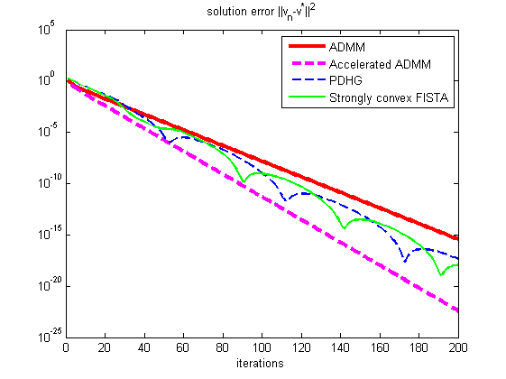
Figure 3 displays the evolution of both measures, as well as the theoretical convergence decays expected in each case ( and ). We chose and , so that .

(a) Objective error
(b) Solution error
We first observe that, as expected, the accelerated ADMM has a better convergence than the unaccelerated ADMM. The empirical rates are better than the theoretical ones, which can be explained by the over-smoothness of the quadratic problem, compared to the assumptions required by the smooth case.
We also observe oscillations for both the oPDHG and strongly convex FISTA. Rippling for FISTA has been already observed for quadratic problems of this kind [16]. This phenomena occurs when the overrelaxation parameter is chosen too large compared to the eigenvalues of . Similar cause may explain the oscillations in the oPDHG, namely using overrelaxation steps can introduce oscillations when the according parameter are unproperly chosen. Hence, we do not expect to observe such oscillations for ADMM-like schemes.
6.2 Denoising with TV-Huber
6.2.1 Problem
We now apply the accelerated ADMM to a denoising problem, which is less smooth and more realistic than the toy example. Let be a RGB-color (noisy) image. We want to solve the following problem:
| (166) |
where the gradient linear operator is defined for any color image by a pair of color images . The finite differences are given at any index by
| (167) |
and
| (168) |
The TV-Huber regularization term is defined by
| (169) |
with
| (170) |
Hence, this term acts like a quadratic regularization when the image variations are small and like a TV regularization when they are larger (see Figure 4). The quantity is a weight parameter.
The convex conjugate of the regularization function can be proved to be
| (171) |
where if and otherwise. This implies that is -convex.


6.2.2 ADMM
Let . We apply the accelerated ADMM to problem (166), which leads to the following iterations:
Each minimization is solved thanks to the Euler equation: the -update reads
| (172) |
whereas the -update is given by
| (173) |
with
| (174) |
6.2.3 Parameters
Before choosing the parameters, we recall the regularity of the problem. Functions and are respectively -convex and -convex. The gradient operator is bounded, of norm (this bound being tight when or go to ). Thus, we set . We tested two sets of parameters:
- 1.
optimal parameter for the unaccelerated ADMM: ;
- 2.
optimal paramters for the accelerated ADMM:
(175)
These choices lead to the convergence rates for the unaccelerated ADMM and for the accelerated one.
6.2.4 oPDHG and strongly convex FISTA
The primal-dual formulation of problem (166) is given by
| (176) |
Hence using the oPDHG algorithm to solve it leads to the following iterations:
| (177) |
which are computed thanks to the Euler equation:
| (178) |
The best choice of parameters for this algorithm is (Theorem 2):
| (179) |
If we apply strongly convex FISTA to this problem, this leads to the following updates:
| (180) |
which leads to the explicit update
| (181) |
The variable relaxation parameter follows the update rule (21) with .
6.2.5 Results
To measure the convergence of the algorithm, we used the same two tools as in the previous case: the solution error and the objective error.
Figure 5(a) displays the evolution of the objective error, while Figure 5(b) shows the decay of the solution error, for the accelerated ADMM and the oPDHG method. In the latter, the theoretical linear rate is also plotted for comparison. We chose . The solution error decreases as expected for all methods except strongly convex FISTA, for which we did not estimate a finer theoretical rate for the solution error. In practice, it seems that it converges with same rate as the oPDHG. Hence, in terms of solution error convergence, the accelerated ADMM provides the best empirical decay. For the objective error, the accelerated ADMM, the oPDHG method and strongly convex FISTA yield comparable decay rate. However, one should keep in mind that both the unaccelerated ADMM and the accelerated ADMM require an operator inversion, unlike the oPDHG method and strongly convex FISTA. Hence, even if comparable number of iterations are needed to achieve convergence, the ADMMs iterations are more time consuming than the other methods and should be used only when the inversion of the operator can be implemented efficiently.

(a) Objective error

(b) Solution error - Comparison with the theoretical rate
7 Conclusion
In this work, we studied the convergence of the oPDHG scheme in the case where the composite problem has a strongly convex part and a differentiable with a Lipschitz continuous gradient part. Using the equivalence between this algorithm and the ADMM, we provided a new convergence analysis of the latter. This analysis allowed us to introduce an accelerated variant of the ADMM by changing the augmented Lagrangian parameter, which is proved to have same convergence rate as the oPDHG method. Hence, we showed that in the smooth case, the choice of the ADMM parameter(s) can be crucial in terms of convergence rate. Experimental results confirmed this theoretical analysis. In particular, it has been observed that the accelerated ADMM does not introduce oscillations in some cases, unlike the oPDHG algorithm and strongly convex FISTA, which are known to be in practice more efficient than the ADMM-like scheme, since they require no operator inversion.
References
- [1] Amir Beck and Marc Teboulle. A fast iterative shrinkage-thresholding algorithm for linear inverse problems. SIAM journal on imaging sciences, 2(1):183–202, 2009.
- [2] Stephen Boyd, Neal Parikh, Eric Chu, Borja Peleato, and Jonathan Eckstein. Distributed optimization and statistical learning via the alternating direction method of multipliers. Foundations and Trends® in Machine Learning, 3(1):1–122, 2011.
- [3] Antonin Chambolle and Thomas Pock. A first-order primal-dual algorithm for convex problems with applications to imaging. Journal of Mathematical Imaging and Vision, 40(1):120–145, 2011.
- [4] Antonin Chambolle and Thomas Pock. On the ergodic convergence rates of a first-order primal–dual algorithm. Mathematical Programming, pages 1–35, 2015.
- [5] Antonin Chambolle and Thomas Pock. An introduction to continuous optimization for imaging. Acta Numerica, 25:161–319, 2016.
- [6] Damek Davis and Wotao Yin. Faster convergence rates of relaxed peaceman-rachford and admm under regularity assumptions. arXiv preprint arXiv:1407.5210, 2014.
- [7] Wei Deng and Wotao Yin. On the global and linear convergence of the generalized alternating direction method of multipliers. Journal of Scientific Computing, 66(3):889–916, 2016.
- [8] Ernie Esser, Xiaoqun Zhang, and Tony F Chan. A general framework for a class of first order primal-dual algorithms for convex optimization in imaging science. SIAM Journal on Imaging Sciences, 3(4):1015–1046, 2010.
- [9] Daniel Gabay and Bertrand Mercier. A dual algorithm for the solution of nonlinear variational problems via finite element approximation. Computers & Mathematics with Applications, 2(1):17–40, 1976.
- [10] Roland Glowinski and A Marrocco. Sur l’approximation, par éléments finis d’ordre un, et la résolution, par pénalisation-dualité d’une classe de problèmes de dirichlet non linéaires. Revue française d’automatique, informatique, recherche opérationnelle. Analyse numérique, 9(2):41–76, 1975.
- [11] Bingsheng He, Yanfei You, and Xiaoming Yuan. On the convergence of primal-dual hybrid gradient algorithm. SIAM Journal on Imaging Sciences, 7(4):2526–2537, 2014.
- [12] Mingyi Hong and Zhi-Quan Luo. On the linear convergence of the alternating direction method of multipliers. arXiv preprint arXiv:1208.3922, 2012.
- [13] Yurii Nesterov. A method of solving a convex programming problem with convergence rate . In Soviet Mathematics Doklady, volume 27, pages 372–376, 1983.
- [14] Yurii Nesterov. Introductory lectures on convex optimization. applied optimization, vol. 87, 2004.
- [15] Robert Nishihara, Laurent Lessard, Benjamin Recht, Andrew Packard, and Michael I Jordan. A general analysis of the convergence of admm. arXiv preprint, 2015.
- [16] Brendan O’Donoghue and Emmanuel Candes. Adaptive restart for accelerated gradient schemes. Foundations of computational mathematics, 15(3):715–732, 2015.
- [17] Thomas Pock, Daniel Cremers, Horst Bischof, and Antonin Chambolle. An algorithm for minimizing the mumford-shah functional. In Computer Vision, 2009 IEEE 12th International Conference on, pages 1133–1140. IEEE, 2009.
- [18] Mingqiang Zhu and Tony Chan. An efficient primal-dual hybrid gradient algorithm for total variation image restoration. UCLA CAM Report, pages 08–34, 2008.