Signal Detection under Short-Interval Sampling of Continuous Waveforms for Optical Wireless Scattering Communication
Abstract
In optical wireless scattering communication, received signal in each symbol interval is captured by a photomultiplier tube (PMT) and then sampled through very short but finite interval sampling. The resulting samples form a signal vector for symbol detection. The upper and lower bounds on transmission rate of such a processing system are studied. It is shown that the gap between two bounds approaches zero as the thermal noise and shot noise variances approach zero. The maximum a posteriori (MAP) signal detection is performed and a low computational complexity receiver is derived under piecewise polynomial approximation. Meanwhile, the threshold based signal detection is also studied, where two threshold selection rules are proposed based on the detection error probability and the Kullback-Leibler (KL) distance. For the latter, it is shown that the KL distance is not sensitive to the threshold selection for small shot and thermal noise variances, and thus the threshold can be selected among a wide range without significant loss from the optimal KL distance. The performances of the transmission rate bounds, the signal detection, and the threshold selection approaches are evaluated by the numerical results.
Key Words: Optical wireless communication, photomultiplier tube (PMT), photon-counting receiver.
I Introduction
Due to the potential large bandwidth and no electromagnetic radiation, optical wireless communication shows great promise for the future wireless communications[1]. It can be deployed for the applications where the radio-frequency (RF) radiation is prohibited, for example in a hospital or aircraft cabin where the electromagnetic radiation is of particular concern. In some outdoor scenarios,, the line-of-sight (LOS) link between the transmitter and the receiver may be blocked by an obstacle, or cannot be guaranteed due to the application requirements. The solution is to utilize the non-line-of-sight (NLOS) optical scattering communication [2, 3], typically in the ultra-violet spectrum. For the NLOS communication, the transmitting and receiving directions are not required to be perfectly aligned, which expands the application range beyond the LOS links. The NLOS optical scattering communication channels and systems have been extensively studied from both experimental perspective [3, 4, 5, 6], and semi-analytical perspective [7, 8, 9].
Due to the large path loss between the transmitter and the receiver, the received signals are characterized by discrete photoelectrons. Using a photon-counting receiver, the number of detected photoelectrons satisfies a Poisson distribution, which forms a Poisson channel. The capacity of the Poisson channel has been studied in [10, 11, 12]. Recently, the capacity and the optimized source distribution for the discrete-time Poisson (DTP) channel have been investigated in [13], [14]. The capacity and signal detection of the free-space MIMO optical wireless communication system based on the ideal photon-counting receiver and maximum-likelihood (ML) detection have been investigated in [15], [16]. The base-band digital signal processing and the coded modulation have been studied in [17, 18, 19]. Besides, the communication channel modeling and signal processing has been investigated, in the aspects of the inter-symbol interference modeling [20], the relay protocol for the photon-counting receiver [21], [22], and the linear receiver for the SIMO scattering communication with Poisson shot noise [23].
Note that the capacity for the Poisson channel is achieved as interval for counting the detected photoelectrons becomes arbitrarily small. However, this cannot be realized in a practical receiver. On the other hand, an ideal discrete photon-counting receiver is difficult to realize, while typically a continuous waveform processing (WP) receiver consisting of a photomultiplier tube (PMT) and postprocessing circuits is employed. The WP receiver amplifies each detected photoelectron to a series of electrons, with the additive signal dependent shot noise and signal independent thermal noise. It becomes interesting to investigate the achievable transmission rate and the signal detection performance of the WP receiver, where interval for measuring the PMT outputs cannot be arbitrarily small.
In this work, we study the transmission rate and the signal detection for such type of practical WP receiver from three perspectives, the transmission rate, the signal detection, and the non-ideal photon-counting receiver based on the hard-decision with a preset threshold. Assume a small but finite time processing interval for measuring the PMT outputs, such that PMT output signals within each symbol duration form a vector consisting of the output signals within the intervals. To the best of our knowledge, such a model has not been analyzed before. We investigate the upper and lower bounds on the transmission rate of such type of channel. We also study the maximum a posteriori (MAP) signal detection for the transmitted symbol, and approximation at reduced computational complexity. Moreover, we consider a non-ideal photon-counting receiver, where a preset threshold is employed for the hard decision on whether a photoelectron exists in each interval. The optimal threshold selection rule is investigated based on two criteria, to minimize the detection error probability and to maximize the Kullback-Leibler (KL) distance. We further prove that for small shot and thermal noise variances, the detection threshold can be selected among a wide range without significant loss from the optimal KL distance. The performances of the proposed transmission rate bounds, the signal detection, and the optimal threshold selection criteria for the non-ideal photon-counting receiver are evaluated by the numerical results.
The remainder of this paper is organized as follows. In Section II, we present the model of the NLOS optical wireless scattering communication system and the PMT output signal. In Section III, we investigate the upper and lower bounds on the communication rate. In Section IV, we consider the MAP detection of the transmitted symbol, and propose a reduced computational complexity receiver. In Section V, we provide the signal model for the non-ideal photon-counting receiver, and obtain the optimal threshold based on the detection error probability and the KL distance. Numerical results are given in Section VI. Finally, Section VII provides the concluding remarks.
II Channel Model
II-A Optical Wireless Scattering Communication with WP receiver
Consider an optical wireless scattering communication system, typically in the ultra-violet (UV) spectrum. Due to the large path loss of the scattering by the particles and aerosol in the atmosphere, the intensity of received signal becomes extremely weak, where the signals are characterized by the discrete photoelectrons. The detected photoelectrons consist of two components, the desired signal component and the background radiation component. The numbers of photoelectrons for both components satisfy Poisson distributions.
Assume that the transmitter adopts on-off keying (OOK) modulation, where denotes the transmitted symbol. Let denote the transmission power for when the transmission is on, and denote the link gain between the transmitter and the receiver. Let and denote the Planck’s constant and the frequency of the optical carrier, respectively, such that the energy per photon is given by . Let denote the detector quantum efficiency as the ratio between the number of photoelectrons over the number of received photons; and denote the length of the OOK symbol duration. The mean number of detected photoelectrons for the desired signal component corresponding to the transmission power , denoted as , is given by
| (1) |
Let denote mean number of detected photoelectrons for the background radiation in each symbol duration. The number of detected photoelectrons, denoted as , satisfies the following Poisson distribution,
| (2) |
Consider a practical PMT detector that amplifies each detected photoelectron into a series of electrons. Let and denote the amplification factor and the charge of each electron, respectively. The PMT output signal upon detecting photoelectrons, denoted as , is given by
| (3) |
where denotes the additive Gaussian noise including the shot noise and the thermal noise. Let and be the variances of the shot noise per photoelectron and the thermal noise, respectively. Note that the additive noise satisfies the Gaussian distribution with mean zero and variance . We have the following on the shot noise per photoelectron the thermal noise variances,
| (4) |
where denotes the PMT spreading factor; denotes the Boltzmann constant; denotes the temperature (); and denotes the load resistance. Let denote the Gaussian probability distribution function (PDF) with mean and variance . The pdf of upon detecting photoelectrons, denoted as , is given as follows,
| (5) | |||||
The pdf of the PMT output signal, denoted as , is given by
| (6) | |||||
II-B The WP receiver with a Finite Processing Time Interval
Note that for the Poisson channel, the capacity is achieved when the receiver can count the number of detected photoelectrons in an arbitrarily small interval. However, this cannot be realized by a practical receiver, where the interval for counting the detected photoelectrons cannot be arbitrarily small. In this work, we assume that the minimum processing interval for the PMT output is given by for some integer . This can be implemented via adopting a high-rate sampling to the PMT output signals, and detecting the transmitted symbol based on the sampled signals within each minimum processing interval.
For each symbol duration, let denote the output analog signal vector of the WP receiver in the intervals. We need to decode the information symbol based on the signal vector of the intervals. Note that the number of detected photoelectrons for each interval satisfies a Poisson distribution, with means and for OOK symbols and , respectively. The conditional pdfs for given and , denoted as and , respectively, are given by
| (7) |
Assume that given , the output signals , , …, are independent of each other. This can be justified by the independent Poisson arrival events and additive Gaussian noise in different intervals. Thus the pdfs of the output signal for and , denoted as and , respectively, are given by
| (8) |
where the conditional pdfs and for are given by (7).
II-C The Single-Photon Approximation
For fixed symbol duration such that and are all fixed, we consider sufficiently small such that both and are small. In such a scenario, for Poisson distributions with means and , the probability for detecting more than one photoelectrons becomes negligible. Then the Poisson distributions can be approximated by Bernoulli distributions. The probability for the detected photoelectron number in a length- interval is given by,
| (9) |
Based on the above approximation and defined in (5), for and , the pdfs of the output signal , , are given by
| (10) |
The single-photon approximation can be justified by the observation on the PMT output signal from the oscilloscope, which is characterized by the discrete pulses corresponding to the detected photoelectrons. Typically if dividing the entire symbol duration into small intervals for a large , there is at most one pulse in each length- interval. The motivation of this work is to detect the OOK symbol based on the output analog signal in each interval. We address such a problem in three perspectives, the communication rate for the OOK modulation, the signal detection, and the non-ideal photon-counting receiver based on the output signal vector .
III The Transmission Rate
Let denote the stochastic variable versions of the signals , , …, . In this Section, we first investigate the mutual information for each interval. It also represents the mutual information per OOK symbol for sufficiently small symbol duration, such that and are sufficiently small for . We provide the upper and lower bounds on the mutual information . Finally we extend the upper and lower bounds to the mutual information for the intervals.
III-A Upper and Lower Bounds on the Transmission Rate for Single Interval
Consider the priori probability, , and . In this subsection, without loss of generality we set . Let , ; and denote the pdf of . Based on the single-photon approximation, the communication rate for a single interval is given by
| (11) | |||||
Consider the transmitted OOK symbol , the number of detected photoelectrons , the PMT output analog signal , and the number of detected photoelectrons inferred from the analog signal , denoted as . We have that forms a Markov chain. Based on this, the mutual information can be bounded as follows:
| (12) |
In the following we analyze the gap between the upper bound and the lower bound. The main result is that the gap attenuates with the summation of shot noise variance and the thermal noise variance in a super-power manner.
Note that both transitions and form binary asymmetric channels. Such type of channel can be characterized by the conditional probabilities and for the output symbol given OOK symbols and . The mutual information is given by
| (13) | |||||
where the entropy function . Note that the bounds and can be obtained based on setting the conditional probabilities and to the corresponding values.
For the binary channel , based on the analysis in Section II.C, we have the following,
| (14) |
For the binary channel , the detection of from the PMT output signal could be performed according to the MAP criterion. However, the complicated expression of the detection threshold is not tractable for further analysis. Thus we resort to a more tractable detection of from the output signal based on a simple detection threshold , such that is detected if , and is detected otherwise. The simple threshold can still lead to the super-linear attenuation of the gap between the upper bound and the lower bound. The typical range of the detection threshold is given by , for example .
In this scenario, the corresponding conditional probabilities and are given by
| (15) | |||||
where denotes the following Gaussian- function
| (16) |
It is easily seen that conditional probabilities and approach and as the shot noise variance and the thermal noise variance approach zero. The upper and lower bounds on the communication rate [c.f. (11)] can be given in the following result.
Proposition 1
The upper and lower bounds on the transmission rate are given as follows,
| (17) |
Moreover, the upper and lower bounds are asymptotically tight as the shot noise variance and the thermal noise variance approach zero, i.e.,
| (18) |
An upper bound on the gap can be obtained based on the following lemma.
Lemma 1
For the Markov chain , we have that
| (19) |
Proof:
We have the following on the mutual information gap ,
| (20) | |||||
∎
In the following we analyze the convergence of the conditional entropy . Letting and , we have that
| (21) |
Letting and , we have the following on the conditional probabilities for and ,
| (22) |
It can be proved that the conditional entropy attenuates with the variances and in the super-power order for both and . More specifically, we have the following result.
Theorem 1
For any , we have the following on the asymptotical results on the conditional entropy ,
| (23) | |||||
| (24) |
Proof:
We provide the proof on as follows. Note that we have the following,
| (25) | |||||
As and for , we have following
| (26) |
| (27) |
Note that and as approaches zero. Thus, we have that and the following bounds for ,
| (28) |
Thus, the limit of condition entropy is bounded by
| (29) | |||||
For , note that contains the exponential term which attenuates with the variances in the super-power order. Based on the above analysis, the rest proof of (23) can be easily derived using the standard arguments on the mathematical analysis.
The proof of (24) for are similar to that for , and thus omitted here. ∎
III-B Upper and Lower Bounds on the Transmission Rate for Multiple Intervals
We extend the previous results to a vector case where M intervals yield a vector output. Let denote the analog PMT output in the intervals. Let denote the stochastic representation of for the mutual information, such that
| (30) |
Similar to that for single interval, let denote the vector of the number of detected photoelectrons in the intervals, and denote the vector of photoelectrons inferred from the signal vector . It can be proved that forms a Markov chain. The mutual information can be bounded as follows,
| (31) |
Note that given , the components of and are independent and identically distributed satisfying Bernoulli distributions. The mutual information of such type of channel can be characterized by the conditional probabilities and for each component being one given the OOK symbol and , respectively. Let be the output of such a channel. The conditional probabilities and are given by
| (32) | |||
| (33) |
where denotes the weight of . The probability , and the entropy is given by
| (34) |
The conditional entropy is given by
| (35) | |||||
The mutual information for such binary asymmetric channel is given by . The upper and lower bounds can be obtained via setting and for and , respectively. The parameters have been given in Section III.A.
Based on the above analysis, we have the following result on the upper and lower bounds on the mutual information .
Theorem 2
The upper and lower bounds on the transmission rate are given as follows,
| (36) |
Moreover, the upper and lower bounds are asymptotically tight as the shot and thermal noise variances approach zero, i.e.,
| (37) |
Similar to Lemma for the single interval scenario, we have following result,
| (38) |
Similar to the scenario for single interval, we have the following results on the conditional entropy . The proof follows the same procedure as that of Theorem , and thus omitted here.
Theorem 3
For any , we have the following asymptotical result on the conditional entropy ,
| (39) |
IV The detection
In this Section, we investigate the MAP detection of the OOK symbols based on the PMT output signal . We also provide a piecewise polynomial approximation for the log-likelihood to reduce the computational complexity.
IV-A The MAP Detection Framework
For the MAP detection of based on the PMT output signal in the intervals , symbol is detected if the following is satisfied
| (40) |
and symbol is detected otherwise. Such a detection rule is equivalent to the rule that is detected if and only if the following is satisfied
| (41) |
Based on the single-photon approximation, is detected if and only if the following is satisfied,
| (42) |
The log-likelihood ratio in (42) can be simplified as follows. Note that we have
| (43) |
where parameters , , and are given by
| (44) |
Letting for , we have the following on the LLR,
| (45) |
Note that in the above summation for each , the numerator and the denominator contain the exponential term . Such detector may suffer a high computational complexity since both the exponential and the logarithm operations are involved. To reduce such complexity, we resort to a piecewise approximation on in terms of , which is provided in the following subsection.
IV-B The Piecewise Approximation for the MAP Detection
We provide piecewise approximations on the function to reduce the computational complexity. We first provide a piecewise linear approximation, which shows virtually the same detection error probability as that of the accurate LLR in the low thermal noise variance regime. To reduce the detection error probability in the high thermal noise variance regime, we further propose a piecewise polynomial approximation up to the cubic term.
We provide the following properties on the function , which will be used in the piecewise approximation.
Theorem 4
We have the following limit on as approaches infinity,
| (46) |
Moreover, we have that is central symmetric on the point , where is given by
| (47) |
In other words, we have that for .
Based on the above properties, we propose the piecewise linear approximation and piecewise cubic polynomial approximation on .
IV-B1 Piecewise Linear Approximation
The piecewise linear approximation is based on three lines, where two lines are the limits of as and , and one line is the tangent line of at the point . More specifically, the three-line piecewise function is given as follows,
| (51) |
where slope , point , and point . As , the three-line piecewise approximation degrades to a two-value step function.
IV-B2 Piecewise Cubic Polynomial Approximation
The entire range of variable is divided into five parts. The function follows approximations using the limits as approaches positive infinity and negative infinity in the leftmost and the rightmost parts, respectively, and using cubic polynomial functions in the three middle parts. The five parts in the entire range of are given by , , , and . The piecewise approximation of is given as follows,
| (52) |
Note that intuitively the divided parts for the piecewise approximation need to be symmetric in terms of the point . However, according to the distribution of , the probability of belonging to is significantly larger than that of belonging to . The approximation accuracy in the region needs to be higher than that in the region . Thus, we divide region into more parts.
Let denote the coefficient vector of the cubic polynomial for . Assume that in each part , equally spaced samples are employed for the approximation. Let , the polynomial approximation is based on the following least squares criterion,
| (53) |
where denotes the probability density of at the point . Here we adopt the probability density as the weight for the approximation. The PDF of is given by,
| (54) |
where can be derived according to the relationship .
Note that the polynomial approximation can be expressed by the following quadratic form,
| (55) |
where the optimal solution is given by
| (56) |
Numerical results show that such a piecewise cubic polynomial approximation can significantly reduce the detection error probability compared with the piecewise linear approximation, especially for a large thermal noise variance.
V Non-ideal Photon-counting Receiver
The ideal photo-counting receiver that counts the number of detected photoelectrons is difficult to implement in practice. Instead, a non-ideal the photo-counting receiver is implemented based on a WP receiver. A hard decision is employed for the PMT output signal within each interval, where a photoelectron is detected if the PMT output is larger than a certain threshold. A crucial question involved is the selection of the optimal threshold, to minimize the detection error probability. To solve this, we propose the threshold selection based on the exact detection error probability and the KL distance.
V-A The Signal Model for a Non-ideal Photon-counting Receiver
Recall that the PMT output signals in the intervals are given by . Let denote indicators on whether a photoelectron is detected in each interval. A threshold is employed for the detection, where each indicator is given by
Note that for OOK symbols and , each component of the corresponding indicator vector satisfies the corresponding binary distributions. The optimal detection between the two vectors is based on the summation of each component of . For symbols and , the probabilities of each component of being one, denoted as and , respectively, are given by
| (60) |
Let be the summation of the indicators. We have that for , , the summation satisfies the following binomial distributions
| (61) |
V-B The Threshold Selection Rules
The optimal detection for such two different binomial distributions are based on the threshold detection on the summation . Note that and are strictly decreasing with respect to . A natural question is to select the optimal threshold that aims to minimize the detection error probability. This can be solved based on two criteria, to minimize the exact detection error probability and to maximize the KL distance between two Bernoulli distributions. As the exact error probability-based criterion might be intractable due to the high computational complexity, the KL distance-based criterion can serve as an low computational complexity solution.
For the exact detection error probability-based criterion, symbol is detected if and only if
| (62) |
We can obtain a detection threshold such that is detected if and is detected otherwise, where the threshold is given by
| (63) |
The probabilities of symbol being detected for and symbol being detected for , denoted as and , respectively, are given by
| (64) | |||||
| (65) |
The optimal threshold, denoted as , can be selected such that the detection error probability is minimized. More specifically, the optimal threshold is given by
| (66) |
The KL distance-based criterion is based on the method of types, where the two binomial distributions correspond to two types according to the Chernoff-Stein Lemma [24]. As the number of intervals approaches infinity, we have the following on the exponents of and ,
| (67) | |||||
| (68) |
The optimal threshold is selected to maximize the minimum KL distance. More specifically, the optimal threshold is given by
| (69) |
V-C Sensitivity Analysis for the Detection Threshold
We focus on the optimal detection threshold that maximizes the minimum KL distance. We provide the upper and lower bounds on the optimal detection threshold, and further prove that for sufficiently small and , a slight deviation from the optimal detection threshold does not significantly decrease the minimum KL distance. This result shows that the minimum KL distance is not sensitive to the detection threshold selection in a practical system.
To prove this, we first obtain the following upper and lower bounds on the optimal detection threshold .
Theorem 5
We have the upper bound and lower bound on the optimal threshold, where parameters and are independent of and , and
| (70) |
Proof:
Please refer to Appendix A. ∎
Based on Theorem , we have the following bounds on the optimal detection threshold .
Theorem 6
For any , we have that for sufficiently small , the optimal detection threshold satisfies
| (71) |
Proof:
First we prove the upper bound. Note that
| (72) | |||||
| (73) | |||||
| (74) | |||||
| (75) |
Note that for the upper bound given in (75), we have that
| (76) |
Then for any , we have that for sufficiently small , .
Next we prove the lower bound. We have that
| (77) | |||||
| (78) |
Given any , we consider sufficient small , such that the following inequality is satisfied based on (78),
| (79) | |||||
∎
Based on Theorem , the following results shows that the crossover probabilities and are not sensitive to the detection threshold .
Theorem 7
For any and , there exists a sufficiently small and such that for , we have that and for any detection threshold .
Proof:
For any and , we have the following for ,
| (80) |
Letting , we have that for ,
| (81) |
According to Theorem , we have that there exists such that for any ,
| (82) |
Consider . Then for , we have
| (83) |
The same procedure can be performed to prove that . ∎
Based on the above result, since and are not sensitive to the detection threshold , the KL distance is also not sensitive. It implies that for sufficient small thermal noise variance and shot noise variance , the detection threshold can be selected between a value larger than and a value smaller than , without substantial performance loss in terms of the KL distances. Such insights show significant values for the detection threshold selection in a practical scattering communication system.
VI Numerical Results
Consider a WP receiver with additive shot noise and thermal noise. Assume that for the shot noise variance , the PMT spreading factor . Define as the ratio between the signal intensity and the background radiation intensity.
Figure 1 compares the transmission rate from the single-photon approximation and the true rate from the Poisson distribution for different thermal noise variance, for the and . It is seen that the rate from the signal-photon approximation can well approximate the true rate for . The same approximation performance of the single-photon approximation can be observed for . However, the gap between the true rate and the approximation becomes non-negligible for and . It is seen that the single-photon approximation works well for the small photon probability up to .
Figure 2 shows the upper and lower bounds on the rate against the SNR for the thermal noise variance , , and . It is seen that the gap between the two bounds becomes negligible for the thermal noise variance , i.e., the PMT amplification factor . Moreover, Figure 3 shows the upper and lower bounds on the rate against the number of intervals for the and the thermal noise variance , , and . Again, it is seen that gap between the two bounds becomes negligible for the thermal noise variance .
Assume that the number of intervals . We compare the piecewise linear approximation and cubic approximation result in Figure 4 for the . It is seen that the gap between true function and cubic approximation function is negligible, while the gap between true function and linear approximation function is significant. Figure 5 shows the error performance against thermal noise variance . It is seen that the detection error for proposed two approximations becomes negligible for the thermal noise variance . However, the performance loss for the linear approximation becomes non-negligible for the thermal variance , while the performance loss for the piecewise cubic polynomial approximation is still negligible for the thermal variance . This can be justified by the fact that for larger thermal noise variance, there is a larger probability of falling into the region with non-negligible gap for the piecewise linear approximation.


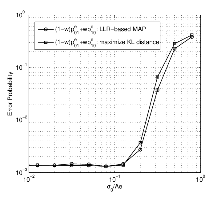
For the non-ideal photon-counting receiver, assume that the symbol duration is divided into slots, and that . The optimal thresholds based on minimizing the detection error probability and maximizing the minimum KL distance are shown in Figure 6. It is seen that the optimal thresholds based on the true detection error probability and the corresponding KL distance are close to each other. Figure 7 compares the detection error probability for the optimal threshold selection based on the exact detection error and the KL distance. It can be seen that threshold selection rule based on the KL distance shows negligible performance loss compared with that based on the exact detection error probability. Moreover, comparing Figure and Figure , we have that the performance loss for the hard-decision of the non-ideal photon-counting receiver is negligible, compared with the optimal LLR based detection. This shows that the non-ideal photon-counting receiver can serve as a good approximation to the optimal receiver, with significantly reduced computational complexity.
Finally, we show the KL distance with respect to the detection threshold in Figure 8 for the values of , and . It is seen that for smaller noise variance, KL distance curve shows larger flat regime including the optimal detection threshold, where the KL distance is less sensitive to the detection threshold . In other words, the small deviation of the detection threshold from the optimal one does not cause substantial performance loss in terms of the KL distance, which validates the results of Theorem .


VII Conclusions
We have modeled the PMT output signal within each symbol duration as a vector of sampled analog signals within small intervals. Based on such a model, we have derived the upper and lower bounds on the transmission rate, which are proved to be tight for the PMT with a large amplification factor and small spreading factor. We have investigated the MAP detector, and the reduced complexity receivers based on the piecewise linear and polynomial approximation. We have also presented a model for the non-ideal photon-counting receiver based on the hard-decision for the PMT output signals. The optimal threshold based on the KL distance is shown to be close to that based on the true detection error probability, with lower computational complexity. Moreover, it is concluded that the non-ideal photon-counting receiver can serve as a good approximation to the optimal receiver, with significantly reduced computational complexity, and the performance is not sensitive to the detection threshold selection for small thermal and shot noise variance.
-A Proof of Theorem 6
We first investigate the detection threshold, denoted as , that maximizes the KL distance . Note that we have
| (84) | |||||
Then at the optimal threshold , we have the following,
| (85) |
where
| (86) |
To simplify the following analysis, we define , , , and .
Note that for , we have . Since , we have the following
| (87) | |||||
Based on the above equation and the definition on and [c.f. (61)], we have the following,
| (88) |
To bound the optimal threshold , we consider function , which is shown to be decreasing with respect to and (the proof is given in Appendix.B). Then we have
| (89) |
Substituting (86) into the above inequality, we have that for the where , the following is satisfied,
| (90) |
Considering the range on the detection threshold, via directly solving (90) we have the following upper bound on the optimal threshold ,
| (91) |
On the other hand, the lower bound on the optimal threshold can also be obtained based on Appendix B. Note that for , we have and , and thus
| (92) |
which leads to , where .
We perform the same procedure for and obtain another constant pair , such that for the optimal detection threshold that maximizes (denoted as ) we have that . Let
| (93) |
We have that the minimum KL distance is strictly increasing with respect to for and strictly decreasing with respect to for , which reveals that the optimal threshold cannot locate in the range of . Therefore we have
| (94) |
-B Proof of and (92)
Consider the function
| (95) |
We have the following on the partial derivatives with respect to and ,
| (96) |
which shows that is strictly decreasing with respect to and .
References
- [1] R. M. Gagliardi and S. Karp, Optical Communications, 2nd ed. John Wiley and Sons, New York, 1995.
- [2] Z. Xu and B. M. Sadler, “Ultraviolet communications: potential and state-of-the-art,” IEEE Commun. Mag., vol. 46, no. 5, pp. 67–73, May 2008.
- [3] H. Ding, G. Chen, A. K. Majumdar, B. M. Sadler, and Z. Xu, “Modeling of non-line-of-sight ultraviolet scattering channels for communication,” IEEE Journal Select. Areas Commun., vol. 27, no. 9, pp. 1535–1544, Sept. 2009.
- [4] H. Ding, Z. Xu, and A. K. Majumdar, “A path loss model for non-line-of-sight ultraviolet multiple scattering channels,” EURASIP Journal Wireless Commun. Networking, vol. 2010, no. 5, pp. 1–12, Jun. 2010.
- [5] H. Xiao, Y. Zuo, J. Wu, H. Guo, and J. Lin, “Non-line-of-sight ultraviolet single-scatter propagation model,” Optics Express, vol. 19, no. 18, pp. 17 864–17 875, Aug. 2011.
- [6] L. Liao, Z. Li, T. Lang, and G. Chen, “UV LED array based NLOS UV turbulence channel modeling and experimental verification,” Optics Express, vol. 23, no. 17, pp. 21 825–21 835, Aug. 2015.
- [7] L. Wang, Z. Xu, and B. M. Sadler, “Non-line-of-sight ultraviolet link loss in noncoplanar geometry,” Optics Letters, vol. 35, no. 8, pp. 1263–1265, Aug. 2010.
- [8] Q. He, Z. Xu, and B. M. Sadler, “Performance of non-line-of-sight LED based ultraviolet communication receivers,” Optics Express, vol. 18, no. 12, pp. 12 226–12 238, May 2010.
- [9] Q. He, B. M. Sadler, and Z. Xu, “On the achievable performance of non-line-of-sight ultraviolet communications,” in Proc. of OSA Topical Meeting on Applications of Lasers for Sensing and Free Space Communications (LSC), San Diego, CA, Jan. 2010.
- [10] A. D. Wyner, “Capacity and error component for the direct detection photon channel - Part I-II,” IEEE Trans. Info. Theory, vol. 34, no. 6, pp. 1449–1471, Nov. 1988.
- [11] M. R. Frey, “Information capacity of the Poisson channel,” IEEE Trans. Info. Theory, vol. 37, no. 2, pp. 244–256, Mar. 1991.
- [12] A. Lapidoth and S. M. Moser, “On the capcity of the discrete-time Poisson channel,” IEEE Trans. Info. Theory, vol. 55, no. 1, pp. 303–322, Jan. 2009.
- [13] J. Cao, S. Hranilovic, and J. Chen, “Capacity-achieving distributions for the discrete-time Poisson channel - part I: General properties and numerical techniques,” IEEE Trans. Commun., vol. 62, no. 1, pp. 194–202, Jan. 2014.
- [14] ——, “Capacity-achieving distributions for the discrete-time Poisson channel - part II: Binary inputs,” IEEE Trans. Commun., vol. 62, no. 1, pp. 203–213, Jan. 2014.
- [15] S. G. Wilson, M. B. Pearce, Q. Cao, and M. Baedke, “Optical repetition MIMO transmission with multipulse PPM,” IEEE Journal Select. Areas Commun., vol. 23, no. 9, pp. 1901–1910, Sept. 2005.
- [16] S. G. Wilson, M. B. Pearce, Q. Cao, and J. H. Leveque, “Free-space optical MIMO transmission with Q-ary PPM,” IEEE Trans. Commun., vol. 53, no. 8, pp. 1402–1412, Aug. 2005.
- [17] A. R. Calderbank and C. N. Georghiades, “Synchronizable codes for the optical OPPM channel,” IEEE Trans. Info. Theory, vol. 40, no. 4, pp. 1097–1107, Jul. 1994.
- [18] N. Chatzidiamantis, G. K. Karagiannidis, and M. Uysal, “Generailized maximum-likelihood sequence detection for photon-counting free space optical systems,” IEEE Trans. Commum., vol. 58, no. 12, pp. 3381–3385, Dec. 2010.
- [19] T. T. Nguyen and L. Lampe, “Coded multipulse pulse-position modulation for free-space optical communications,” IEEE Trans. Commum., vol. 58, no. 4, pp. 1036–1041, Apr. 2010.
- [20] C. Gong and Z. Xu, “Channel estimation and signal detection for optical wireless scattering communication with inter-symbol interference,” IEEE Trans. Wireless Commun., vol. 14, no. 10, pp. 5326–5337, Oct. 2015.
- [21] Q. He, Z. Xu, and B. M. Sadler, “Non-line-of-sight serial relayed link for optical wireless communications,” in Proc. 2010 IEEE Military Communications Conference, San Jose, CA, Oct. 31-Nov. 3, 2010.
- [22] C. Gong and Z. Xu, “Non-line-of-sight optical wireless relay with photon counting receiver: A count-and-forward protocol,” IEEE Trans. Wireless Commun., vol. 14, no. 1, pp. 376–388, Jan. 2015.
- [23] ——, “LMMSE SIMO receiver for short-range non-line-of-sight scattering communication,” IEEE Trans. Wireless Commun., vol. 14, no. 10, pp. 5338–5349, Oct. 2015.
- [24] T. M. Cover and J. A. Thomas, Elements of Information Theory, 2nd ed. Wiley Interscience, 2006.