Simulation of waviness in neutron guides
Abstract
As the trend of neutron guide designs points towards longer and more complex guides, imperfections such as waviness becomes increasingly important. Simulations of guide waviness has so far been limited by a lack of reasonable waviness models. We here present a stochastic description of waviness and its implementation in the McStas simulation package. The effect of this new implementation is compared to the guide simulations without waviness and the simple, yet unphysical, waviness model implemented in McStas 1.12c and 2.0.
1 Introduction
Neutron reflecting guides are most valuable to neutron scattering science, since they transport the neutrons from the source (moderator) surroundings to a low-background region, often 20 to 100 meters away. For time-of-flight neutron instruments, also the sheer instrument length is of value, since it gives an important contribution to improving the instrument resolution.
It is common experience that the transport efficiency of neutron guides degrades with their length. This can partially be explained by multiple reflections, causing unavoidable losses even when using mirrors with almost-perfect reflectivity. However, recent designs of elliptic, parabolic, and other types of ballistic guides Böni (2008); Schanzer et al. (2004); Mühlbauer et al. (2006); Bertelsen et al. (2013); Cussen et al. (2013) have been able to reduce the number of reflections dramatically. Much simulation work has been performed along these routes, and also the first physical realizations of elliptical guides have proven of great benefit Ibberson (2009); Chapon et al. (2011).
Other causes of loss in neutron guide transport are imperfections of the guides, like misalignment or waviness. The effect of misalignment has to some extent been understood for straight guides Allenspach et al. (2001), and back-of-the-envelope calculations show that present-day values of waviness are unproblematic for straight guides. However, concerns have been raised about the severity of imperfect guide conditions for complex guide shapes like the parabolic or elliptic ones. The actual relevance of this is emphasized, as these ballistic guide types are foreseen to be used for a significant part of the instruments at the European Spallation Source (ESS), with guide lengths up to 165 m Source (2013); Klenøet al. (2012).
Simulation of guide waviness has until now been hampered by the lack of a trustworthy description of waviness from individual mirrors, and simple attempts have been found to give physically invalid results Klenø (2013) as we will discuss in the following. We here suggest an approximate model for waviness and present the implementation within the McStas package Lefmann and Nielsen (1999); Willendrup et al. (2014). We will present and discuss the relevant effects of waviness: reflection angle, illumination corrections, mirror shading, and multiple reflections. Finally, we show the effect of waviness in a few realistic guide systems. Our aim with this work is to provide an effective description of the reflectivity as a function of waviness.
1.1 Description of reflectivity and waviness
In most neutron ray-tracing packages, the specular reflectivity of neutron guides is modeled by a piecewise linear function Lefmann and Nielsen (1999); P. Willendrup and Lefmann (2011) that depends only on the length of the neutron scattering vector, :
| (1) |
where the critical scattering vector for natural abundance Ni is Å-1. Expressions with quadratic terms in have also been used with only minor changes in performanceJacobsen et al. (2013); Jacobsen et al. (2014).
For a perfect surface, the low- reflectivity is unity, . However, roughness on length scales smaller than the neutron coherence length will reduce the reflectivity from this value, typical values lie in the range .
What we here understand as waviness is a local deviation of the surface normal of the neutron guide, on the sub-mm to cm range, larger than the neutron coherence length. At this length scale, one can assume that the neutron reflects from a single point at the surface. Typical mean waviness values (FWHM) are of the order to radians Schanzer ().
In our description of waviness, we assume that the whole guide substrate and coating have the same angular deviation as the guide surface. Hence, the reflectivity function, , depends only on the scattering vector and is unaffected by waviness. Instead, waviness affects the angle between the neutron and the guide surface at the reflection point. Thereby it also changes the value of and the direction of the neutron after reflection - with direct consequences for the transport properties of the guide. We assume that all rays are reflected at the surface of the guide piece, effectively this means that we assume that each layer of the supermirror has the same profile as the surface.
2 An algorithm for waviness simulations
As we are only interested in an average description of waviness, we require that the guide waviness can be described stochastically. In other words, we do not need to create and store a complete description of the guide surface height on sub-mm scaled grid. In addition, we require the algorithm to be scale invariant, i.e. it does not depend upon the length scale of the waviness, only on the root-mean-square waviness value, .
When discussing the waviness problem we will solely focus on the longitudinal waviness, i.e. the waviness from rotation around on the axis transverse to the neutron beam path. The transverse waviness will not affect the illumination but only contribute through a very small alteration of the beam direction, which we will ignore in this analysis.
As an introduction, we describe the presently used, but physically wrong algorithm, that nevertheless fulfills these requirements. We investigate by analytics and simple ray-tracing what causes the algorithm to fail, and use this as a starting point to suggest a series of improvements in order to reach an algorithm that is in correspondence with the ray-tracing results.
2.1 The Gaussian waviness model
A somewhat inaccurate stochastic algorithm for the simulation of waviness was implemented in McStas 1.12c in the component Guide_wavy P. Willendrup and Lefmann (2011). The main steps are:
- 1.
Calculate the intersection point between the neutron and the average guide surface.
- 2.
Calculate the angle of incidence with the average guide surface using the guide normal vector and the direction of the incoming neutron wave vector .
- 3.
Rotate n by a random angle, sampled from a Gaussian distribution of width to reach the local surface normal .
- 4.
Calculate the exit angle, , and the final neutron wave vector, , by requiring specular (and elastic) reflectivity of the modified surface, see Fig. 1.
- 5.
Calculate and and use this to modify the beam intensity.
However plausible, this algorithm yields unphysical results. The problem lies in step 3. The probability for the neutron ray to intersect the guide surface is implicitly assumed not to depend upon the local guide normal vector (from now on denoted the local waviness value). This leads to highly unphysical situations. For example, the neutron may reflect from a surface which is locally parallel to . In addition it will be possible for low values to generate negative values of .
2.2 Analysis of the beam illumination of a wavy surface


In order to arrive at a waviness algorithm based on a stochastic theorem, we start by accounting for the beam illumination. The total illumination of a neutron ray of nominal incidence angle on a guide piece of length is
| (2) |
as we everywhere work in the small-angle approximation. We now imagine that the relative height of the guide surface can be written as , where we use periodic boundary conditions, . We use the McStas convention where is along the main neutron flightpath. The local inclination is then given as . The local illumination of this piece of guide of length can in the small angle approximation be written as
| (3) |
The probability for a general neutron ray to reflect from this particular piece of guide is its fraction of the total illumination
| (4) |
The integral of (4) over the full length of the guide piece, , gives
| (5) |
as the integral over vanishes due to the periodic boundary conditions of . In addition, we note that our model is scale invariant, as it depends only on the values of , whose magnitude is determined by the waviness , and not on the guide piece length, .
A necessary requirement for describing a correct waviness reflectivity algorithm is to be able to sample the local inclination according to the probability distribution (4). However, for small values of , (4) can give the unphysical value . This implies that the local inclination angle of the guide surface is higher than the incoming angle. Thus, this part of the surface cannot be reached, as illustrated in Fig. 2. In fact, this implies that also other parts of the guide surface are out of reach, or ”shaded”. Also for the shaded part of the guide surface, the physical reflection probability must be zero, . The figure also shows that the condition for the end of the shaded region is , corresponding to
| (6) |
where and are the beginning and end of the shaded region, respectively. Hence, by replacing by zero in the shaded region, (5) is still fulfilled, which was also verified numerically. This replacement of is shown in Fig. 3 for the particular guide profile example shown in the right part of Fig. 2. Here, the shaded region is between and 46.6 mm is assigned the corrected value .
We choose, without loss of generality, to shift the endpoints of the periodic static surface so that the function does not cause shading at the upper end of the interval.


2.3 A static model for random wavy surfaces
In order to simulate the effects of shading in wavy surfaces, we must be able to generate these surfaces. Waviness is a random phenomenon arising when manufacturing the neutron guide surfaces. It therefore makes sense to model waviness as a stochastic process (See for instance Cox and Miller (1965)) along the length of the guide surface.
Our starting assumption is that the height variations of the imperfect surface may be written as a sum of independent stochastic processes with amplitudes and random phases :
| (7) |
which means that waviness may be expressed as:
| (8) |
This definition may obviously be interpreted as a Fourier series of the surface profile. Denoting the distribution of the phases by the expectation, , of the part processes is:
| (9) |
If we now assume the random phases to be uniformly distributed, the expectation of the sum process . Similarly, the autocovariance function of the sum process (8) is:
| (10) |
where each of the elements in the sum is
| (11) | ||||
| (12) | ||||
| (13) |
Thus,
| (14) |
which also proves that the sum process is stationary as the autocovariance function only depends on the distance between two samples, not on the absolute location along . The stationarity property also proves our earlier statement that we may choose to shift the generated surface so we avoid shading in the beginning of the considered interval.
Waviness, , is generally specified as a standard deviation of the angle variations along the length of a guide. In terms of the defined stochastic process, this is simply . What remains is to define the amplitudes (or Fourier coefficients) of the part processes. The spectral properties hereof must depend on the actual neutron guide manufacturing procedure. For simplicity, here we choose
| (15) |
which indicates a fairly uniform weighting of low frequency components while suppressing high frequency variations, which are generally not significant for the purpose of describing waviness. To simulate a guide, we generate a realization of equation (8) with amplitude coefficents given by (15) normalized to the desired waviness using (14). It is worth to notice that this model is scale invariant and only depends on , hence all profile simulations have been scaled to reasonable length scales P. Böni, D. Clemens, H. Grimmer, and H. Van Swygenhoven (1995). The surface profiles in Fig. 2 and in the remainder of this report are generated in this way, using and . At these values the results converged. A fully stochastic description of waviness should also allow for random fluctuations in the amplitude coefficients, but as we will show in the following, the proposed model, while simple, works quite well and is a significant improvement to the schemes that have been used so far.
2.4 Simulation of shading effects in the static, random model
We have performed simulations of waviness shading on a series of surfaces. For each surface, we have calculated and used weighted histograms to calculate the probability function , describing the frequency each surface orientation is getting hit by the neutron ray. Figure 4 shows the result from one such simulation with a low incidence angle, . The peaks in corresponds to the positions where the local waviness profile is peaking. As expected from the illumination analysis, vanishes below the value .


However, Fig. 4 shows only a single surface. For a stochastic model, all surface patterns should be represented. We simulate this by generating the average of over a large number of static surfaces. Such an average is seen in Fig. 5b. We immediately notice that the distribution vanishes at as it should, and that it otherwise seems like a skewed Gaussian with a center slightly larger than zero.
A simple test expression to model the simulated distribution of is found by multiplying a normal distribution of with the illumination probability (4):
| (16) |
In figure 5, we have overlaid a scaled version of the function (16) to the simulated data, and the agreement is found to be surprisingly good. For small incidence angles, , there are small deviations at low values of , where the simulated waviness is lower than the model, which in effect shifts the simulated waviness slightly to the right. This is an effect of the shading, which preferably appear at low values reducing the reflectivity. Figure 5 also shows similar comparisons for higher values of the beam incidence angle. For or higher, the right-shift has almost vanished. This validates the picture of shading as the cause of the right-shift. We have not found a (simple) functional form of that matches the simulated distribution better than eq. (16).


2.5 Correction for multiple reflections
Unfortunately, knowledge about the distribution of the waviness angle is insufficient to constitute a complete waviness algorithm. In addition, we must account for the neutron rays that are reflected multiple times. The necessity for this originates from a simple consideration: Imagine a beam of nominal incident angle being reflected at the local waviness angle . Then, the local angle of incidence is , leading to an outgoing angle of
| (17) |
(See Fig. 1). For negative values of this may result in negative values of , meaning that the neutron ray continues down towards the mirror. With the exception of reflections at the very end of the mirror, there will be (at least) one other reflection before the neutron ray has left the mirror.
To quantify the effect of this, we have employed a simple ray-tracing method when simulating the wavy surfaces. We chose the initial intersection point in accordance with the illumination and shading discussed above and construct the angle of the outgoing neutron ray according to (17). We then follow the outgoing ray over an extended surface that spans over a length of . We check across the surface height curve if the ray collides with the surface again. If there is such a multiple collision, another outgoing angle is calculated according to (17), and the ray-tracing continues. Two examples of these simulations are given in Fig. 6.


We have performed a series of simulations with varying incident angles, , with simulations per angle, to obtain the fraction of multiply reflected rays. The results are shown in Fig. 7. We observe that the degree of multiple reflection is highest, just below 10%, for , to decay to zero for , and for angles higher than . This is in agreement with expectations, since rays with very low angles will reflect only from the tops of the height curve, , on the side with due to shading, while high incident angles will reflect with high outgoing angles without chance for having a second reflection, , leaving eq. (17) always positive. Fig. 7 also shows that the ratio of rays with more than two reflections in general behaves as the ratio of all multiple reflections. The maximum is of the order 1%, occurring also around .

Our most important result, however, is the distribution of final reflections angles, . A naive prediction of the shape of this simulation would come from taking only the illumination argument into account, ignoring shading and multiple scattering. Here we combine (16) and (17) to reach
| (18) |
Fig. 8b shows the simulated distribution overlaid with the eq. (18). We observe that the simulations show a vanishing probability for a reflection at , as one must require, while the naive prediction (18) has a finite probability at negative values, as it does not include multiple reflections.
The full analytical description of the illumination, shading, and multiples into one equation is a complex task that we have no intention of performing. However, we have performed a minimal change of (18) to make it vanish at :
| (19) |
Fig. 8 show that this equation in fact describes the simulated distribution of the outgoing angle quite well for . Hence, we use (19) as a first order conjecture for the true outcome of the reflection from wavy surfaces.
We have as well performed simulations of other values of : 0.5, 2, and 4. All these results are shown along with the predictions (18) and (19) in Fig. 8. We see that for the high angles of incidence, , the naive prediction (18) in general works better than the conjecture (19).


3 A new approximate algorithm for waviness simulation
Our objective is now to find a functional form that can effectively describe as a function of and . From our simulations we see that approaches zero for . For small it increases linearly with to a maximum slightly above and then decreases in a Gaussian manner. In the other end of the spectrum, when is large, can be described by a Gaussian with a width centered at . Both observations are in accordance with the simple considerations discussed earlier. We have made no attempt to understand the details the shape of in the intermediate region.
As a starting point we have modified the expression (18) in order to reproduce the observed behavior. We have produced three alternatives:
| (20) | ||||
| (21) | ||||
| (22) |
where and are the dimensionless variables and respectively.
A series of simulations with going from 0.22 to 10 was made and each simulation was fitted to the expressions (20), (21) and (22). In all cases the , and are fitting parameters that are free to vary. Fig. 9 shows the root mean square of the residuals for each fit. It is clear that the expression has the best performance over the whole range. This can also be seen in the individual simulations, in Fig. 10 examples where , 1, 2.5 and 4.5 are shown. We therefore choose as our model for describing when simulating waviness.


The value of the fitting parameters , and varies with . In order to make an algorithm that provides for any given , the dependence of the parameters , and was each fitted to an effective model that could approximate the numerical results. This turned out to be:
| (23) |
The results for each expression in (23) can be seen in Fig. 11 and the corresponding parameters in table 1.
| 0.0527 | 0.0162 | 2.6 | 0.0205 | ||||
| 0.395 | 2.5 | 0.076 | 0.541 | 1.9 | 0.007 | 11 | |
| 0.61 | 1.39 |
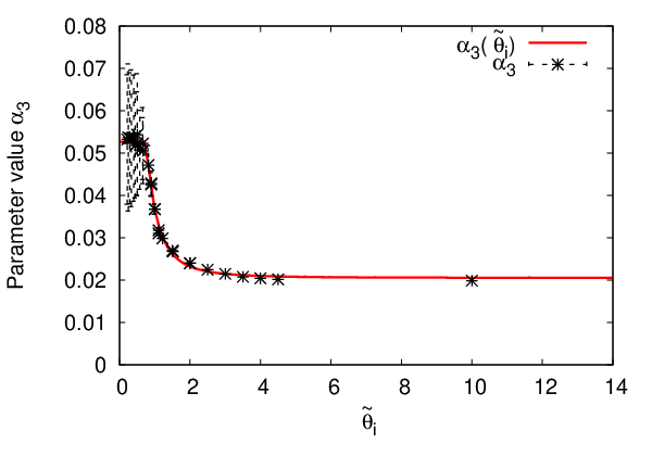
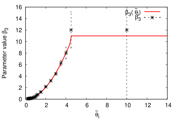
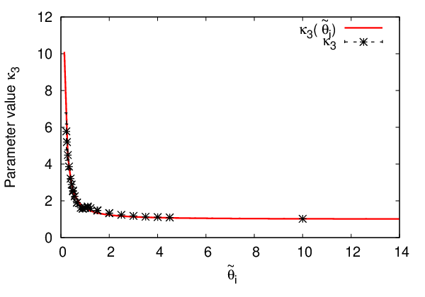
The validity of this model is tested by its strength to predict the simulations made in section 2.5. In Fig. 12 the new model is compared to that of McStas 1.12c for , 1, 2.5 and 4.5. The results from the new model over the whole range are sufficiently close to the simple ray tracing simulations that we do not need to refine the model further.
It should be noted that in the McStas 1.12c model, described in section 2.1, the parameter was taken to be the width of the distribution of final angles. In the new model is the average inclination (rms) of the surface, which gives a width of . We have corrected for this in our comparison in Fig. 12.


4 Implementation of waviness in McStas
The algorithm describing from eq. (22) along with a hit and missCowan (1998) sampling routine, were implemented in a straight guide in McStas. First the outcome of a single reflection from a wavy surface for an extremely narrow and well collimated beam was compared to the simulations made in section 2.5. Fig. 13 shows examples for and . The implementation of waviness in McStas clearly reproduces the simulations from section 2.5.


4.1 Example guide simulations
At last, we show simulations of a 150 m long straight guide with a cross section of starting 4 m from a moderator using only 4 Å neutrons. The guide has a coating described by (1) with , , , and . Simulations were done without waviness, with the McStas 1.12c waviness description (see section 2.1) and with the new description developed in section 3, respectively.


When simulating long neutron guides, there is a significant difference between the new and the McStas 1.12c waviness descriptions for large waviness values, rad, as shown in Fig. 14. In the old version we see a large unphysical peak around divergence which would lead to a brilliance transfer (defined as neutron flux within a small divergence interval and wavelength interval) larger than unity. This, in turn is a violation the Liouville theoremLandau et al. (1980). The reason for this is the oversampling of low values of caused by a mistake in the algorithm.
The main consequence of waviness is in the case of the new description reduced intensity as expected, but no violation of the Liouville theorem. The difference between the two descriptions diminishes for smaller values of , an example with a very low waviness rad is also shown in Fig. 14.
5 Summary
We have performed analytical and simple ray-tracing analysis of the waviness problem relevant for simulations of neutron supermirror reflectivity. The simulations provided a distribution of outgoing angles for a given incoming angle and waviness. It was found that the shape of the distribution evolved as a function of incoming angle.
For each incident angle the distribution was fitted to a expressions whose parameters was taken to be dependent on the incoming angle. This dependence was fitted as well, which resulted in an effective description of the simulated probability distribution of outgoing angles as a function of the incoming angles and waviness.
A routine sampling of the outgoing angle for a given incoming angle and waviness was implemented in a straight-guide component in McStas. There is good accordance between the McStas simulations of a single reflection on a wavy surface of a narrow beam and the ray-tracing simulations described in this work.
The unphysical behavior of the McStas 1.12c waviness model for large waviness values is no longer present in the new model. Instead, the main consequence of waviness is a reduced intensity as expected from simple physical arguments.
Acknowledgements
This project has been funded by the University of Copenhagen 2016 program through the project CoNeXT. CoNeXT is a University of Copenhagen interfaculty collaborative project, which is fertilising the ground and harvesting the full potential of the new neutron and X-ray research infrastructures close to Copenhagen University. We also thank the Danish Agency for Research and Innovation for their support through the contribution to the ESS design update phase.
References
- Allenspach et al. [2001] P. M. Allenspach, P. Böni, and K. Lefmann. Loss mechanisms in supermirror neutron guides. Proc. SPIE, 4509:157–165, November 2001. doi: 10.1117/12.448070. URL http://dx.doi.org/10.1117/12.448070.
- Bertelsen et al. [2013] M. Bertelsen, H. Jacobsen, U. B. Hansen, H. H. Carlsen, and K. Lefmann. Exploring performance of neutron guide systems using pinhole beam extraction. Nuclear Instruments and Methods in Physics Research Section A: Accelerators, Spectrometers, Detectors and Associated Equipment, 729:387–398, November 2013. ISSN 0168-9002. doi: 10.1016/j.nima.2013.07.062.
- Böni [2008] P. Böni. New concepts for neutron instrumentation. Nuclear Instruments and Methods in Physics Research Section A: Accelerators, Spectrometers, Detectors and Associated Equipment, 586(1):1–8, February 2008. ISSN 01689002. doi: 10.1016/j.nima.2007.11.059.
- Chapon et al. [2011] L. C. Chapon, P. Manuel, P. G. Radaelli, C. Benson, L. Perrott, S. Ansell, N. J. Rhodes, D. Raspino, D. Duxbury, E. Spill, and J. Norris. Wish: The New Powder and Single Crystal Magnetic Diffractometer on the Second Target Station. Neutron News, 22(2):22–25, 2011. ISSN 1044-8632. doi: 10.1080/10448632.2011.569650.
- Cowan [1998] G. Cowan. Statistical data analysis. Clarendon Press ; Oxford University Press, Oxford; New York, 1998. ISBN 0198501560 9780198501565 0198501552 9780198501558.
- Cox and Miller [1965] D. R. Cox and H. D. Miller. The theory of stochastic processes. Chapman & Hall, 1965.
- Cussen et al. [2013] L.D. Cussen, D. Nekrassov, C. Zendler, and K. Lieutenant. Multiple reflections in elliptic neutron guide tubes. Nuclear Instruments and Methods in Physics Research Section A: Accelerators, Spectrometers, Detectors and Associated Equipment, 705:121–131, March 2013. ISSN 01689002. doi: 10.1016/j.nima.2012.11.183. URL http://linkinghub.elsevier.com/retrieve/pii/S0168900212015306.
- Ibberson [2009] R. M. Ibberson. Design and performance of the new supermirror guide on HRPD at ISIS. Nuclear Instruments and Methods in Physics Research Section A: Accelerators, Spectrometers, Detectors and Associated Equipment, 600(1):47–49, February 2009. ISSN 0168-9002. doi: 10.1016/j.nima.2008.11.066. URL http://www.sciencedirect.com/science/article/pii/S0168900208016550.
- Jacobsen et al. [2013] H. Jacobsen, K. Lieutenant, C. Zendler, and K. Lefmann. Bi-spectral extraction through elliptic neutron guides. Nuclear Instruments and Methods in Physics Research Section A: Accelerators, Spectrometers, Detectors and Associated Equipment, 717:69–76, July 2013. ISSN 01689002. doi: 10.1016/j.nima.2013.03.048.
- Jacobsen et al. [2014] H. Jacobsen, K. Lieutenant, C. Zendler, and K. Lefmann. Corrigendum to “bi-spectral extraction through elliptic neutron guides” [nucl. instr. and meth. a 717 (2013) 69–76]. Nuclear Instruments and Methods in Physics Research Section A: Accelerators, Spectrometers, Detectors and Associated Equipment, 743:160, April 2014. ISSN 01689002. doi: 10.1016/j.nima.2014.01.024. URL http://linkinghub.elsevier.com/retrieve/pii/S0168900214000400.
- Klenø [2013] K. H. Klenø. Exploration of the Challenges of Neutron Optics and Instrumentation at Long Pulsed Spallation Sources. PhD thesis, University of Copenhagen, 2013.
- Klenøet al. [2012] K. H. Klenø, K. Lieutenant, K. H. Andersen, and K. Lefmann. Systematic performance study of common neutron guide geometries. Nuclear Instruments and Methods in Physics Research Section A: Accelerators, Spectrometers, Detectors and Associated Equipment, 696:75–84, December 2012. ISSN 01689002. doi: 10.1016/j.nima.2012.08.027.
- Landau et al. [1980] L. D Landau, L. P. Pitaevskii, and E. M. Lifshitz. Statistical physics. Butterworth-Heinemann, Oxford [etc.], 1980. ISBN 0750633727 9780750633727.
- Lefmann and Nielsen [1999] K. Lefmann and K. Nielsen. McStas, a general software package for neutron ray-tracing simulations. Neutron News, 10(3):20–23, 1999. ISSN 1044-8632. doi: 10.1080/10448639908233684.
- Mühlbauer et al. [2006] S. Mühlbauer, M. Stadlbauer, P. Böni, C. Schanzer, J. Stahn, and U. Filges. Performance of an elliptically tapered neutron guide. Physica B: Condensed Matter, 385-386:1247–1249, November 2006. ISSN 09214526. doi: 10.1016/j.physb.2006.05.421.
- P. Böni, D. Clemens, H. Grimmer, and H. Van Swygenhoven [1995] P. Böni, D. Clemens, H. Grimmer, and H. Van Swygenhoven. Morphology of Glass Surfaces: Influence on the Performance of Supermirrors. Proceedings of ICANS-XIII, pages 279–287, 1995.
- P. Willendrup and Lefmann [2011] E. Farhi P. Willendrup, E. Knudsen and K. Lefmann. User and programmers guide to the neutron ray-tracing package mcstas, version 1.12, 2011.
- [18] C. Schanzer. Waviness of neutron guides/mirror optics. personal communication, SwissNeutronics.
- Schanzer et al. [2004] C. Schanzer, P. Böni, U. Filges, and T. Hils. Advanced geometries for ballistic neutron guides. Nuclear Instruments and Methods in Physics Research Section A: Accelerators, Spectrometers, Detectors and Associated Equipment, 529(1–3):63–68, August 2004. ISSN 0168-9002.
- Source [2013] The European Spallation Source. ESS technical design report, 2013.
- Willendrup et al. [2014] P. Willendrup, E. Farhi, E. Knudsen, U. Filges, and K. Lefmann. Mcstas: Past, present and future. Journal of Neutron Research, 17(1):35–43, 2014.