Defective Galton-Watson processes

The classical Galton-Watson process (GW-process) is a discrete time Markov chain $Z(\cdot)$ with the state space $\{0,1,\ldots\}$ defined recursively by

$$Z(0)=1,\quad Z(t+1)=\sum_{j=1}^{Z(t)}\nu_{t,j},\quad t=0,1,\ldots,$$

(1)

where $\nu_{t,j}\stackrel{{\scriptstyle d}}{{=}}\nu$ are independent random variables with a common distribution

$$f(s)=Es^{\nu}=\sum_{k\geq 0}p_{k}s^{k}.$$

(2)

In terms of probability generating functions, the branching property (1) yields

$$Es^{Z(t)}=f(t,s),\quad f(0,s)=s,\quad f(t+1,s)=f(f(t,s)),\quad t\geq 0.$$

(3)

There are two types of trajectories for this simple demographic model: a GW-process either becomes extinct at time $T_{0}=\inf\{t\geq 1:Z(t)=0\}$ or $Z(t)\to\infty$ as $t\to\infty$. It is well known that the corresponding probability of extinction $q=P(T_{0}<\infty)$ is given by the smallest non-negative root of the equation $f(s)=s$, see [2, Ch I.5]. Much of the theory of branching processes is devoted to the limit behavior of $Z(t)$ conditioned on $T_{0}>t$ as $t\to\infty$, see [6].

This paper deals with defective GW-processes having $f(1)\in(0,1)$. We treat the defect $\varepsilon=1-f(1)$ of the reproduction law (2) as the probability that a given particle at a given time $t$ sends the Markov chain $Z(t+1)$ to an additional graveyard state $\Delta$. Thus, a defective GW-process becomes a Markov chain with a countable state space $\mathbb{N}_{\Delta}=\{0,1,\ldots\}\cup\{\Delta\}$. Two of the states are absorbing: the process either becomes extinct at time $T_{0}$, or is stopped at time $T_{\Delta}=\inf\{t\geq 1:Z(t)=\Delta\}$. If $T=T_{0}\wedge T_{\Delta}$ denotes the ultimate absorption time, then for some $q\in[0,1)$,

$$P(T_{0}<\infty)=q,\quad P(T_{\Delta}<\infty)=1-q,\quad P(T<\infty)=1.$$

Applying the graveyard absorption properties

$$\Delta+x=\Delta,\quad x\in\mathbb{N}_{\Delta},\qquad s^{\Delta}=0,\quad s\geq 0,\qquad\sum_{j=1}^{\Delta}x_{j}=\Delta,\quad x_{j}\in\mathbb{N}_{\Delta},$$

to the recursion (1), we obtain again (3) implying $f(q)=q$. Clearly, $P(Z(t)=\Delta)=1-f(t,1)$, and if $q=0$, then $T=T_{\Delta}$. It is straightforward to see that

$$E(s^{Z(t)};T_{\Delta}>t)=f(t,s),\quad E(s^{Z(t)};T>t)=E(s^{Z(t)};T_{0}>t)=f(t,s)-f(t,0),$$

since

$$E(s^{Z(t)};T\leq t)=E(s^{Z(t)};T_{0}\leq t)=P(Z(t)=0)=f(t,0).$$

This implies,

	$\displaystyle P(t<T_{\Delta}<\infty)$	$\displaystyle=f(t,1)-q,$
	$\displaystyle P(t<T_{0}<\infty)$	$\displaystyle=q-f(t,0),$
	$\displaystyle P(T>t)$	$\displaystyle=f(t,1)-f(t,0).$

The main focus of this paper is the asymptotic distribution of $Z(t-k)$ conditioned on the survival event $\{T>t\}$ as $t\to\infty$, with $k\in[0,t]$ either being fixed or going to infinity. In Section 2 we present limit theorems assuming that the reproduction law $f(\cdot)$ is fixed. We will see that with fixed $f(\cdot)$, there are two different asymptotic regimes depending on whether $\gamma>0$ or $\gamma=0$, where $\gamma=f^{\prime}(q)$. The proofs of the results of Section 2 are collected in Section 5.

In realistic settings, the defect $\varepsilon$ of the reproduction is small and therefore it is interesting to find asymptotic results as $t\to\infty$ and $\varepsilon\to 0$. To address this issue in Sections 3 and 4 we consider sequences of defective GW-processes $(Z_{n}(\cdot))_{n\geq 1}$ governed by reproduction laws $f_{n}(\cdot)$ such that $\varepsilon_{n}\to 0$ as $n\to\infty$ and $f_{n}(s)\to\hat{f}(s)$ uniformly over $s\in[0,1]$, where $\hat{f}(1)=1$. It turns out that with this approach, a key parameter determining the limit behavior is not $\gamma$ as in Section 2, but rather $\hat{m}=\hat{f}^{\prime}(1)$. We assume $\hat{m}>1$ and even consider the case $\hat{m}=\infty$. The proofs of the results of Sections 3 and 4 are collected in Section 6.

Earlier, a special subclass of the defective GW-processes, the so-called GW-processes with killing, was studied in [5, 7]. A GW-process with killing has a reproduction law of the form $f(s)=g(\alpha s)$, where $g(\cdot)$ is a non-defective generating function and $\alpha\in(0,1)$. In this case $f(1)\in(0,1)$ and $f(s_{0})=1$ for $s_{0}=1/\alpha>1$. To see a counterexample violating the latter restriction, consider

$$f_{0}(s)=1-(p_{1}\sqrt{1-s}+1-p_{1})^{2},\quad s\in[0,1],$$

(4)

having $f_{0}(1)=p_{1}(2-p_{1})$ and

$$f_{0}(t,s)=1-(p_{1}^{t}\sqrt{1-s}+1-p_{1}^{t})^{2}.$$

Since $f^{\prime}_{0}(1)=\infty$, the generating function $f_{0}(s)$ is not defined for $s>1$. Example (4) belongs to a parametric family of defective generating functions with explicit iterations: in [9] the corresponding family of GW-processes is called theta-branching processes. We turn to the theta-branching processes in Section 4. A broad class of continuous time defective branching processes was investigated in [8].

Defective GW-processes arise naturally in the framework of some special non-defective GW-processes with countably many types. For example, the authors of [3] construct an embedded defective GW process in which absorption in the graveyard state corresponds to local survival of the GW-process with countably many types, and absorption in state 0 corresponds to its global extinction. In another multi-type setting, [10] treat the defect $\varepsilon$ as the probability of a favorable mutation allowing a population of viruses to escape extinction.

Notice that the defective GW-processes can be put into the framework of $\phi$-branching processes using a random control function

$$\phi(k)=\left\{\begin{array}[]{llr}k&\text{with probability}&(1-\varepsilon)^{k},\\ \Delta&\text{with probability}&1-(1-\varepsilon)^{k},\end{array}\right.\quad k\geq 0,$$

cf. [11]. Indeed, in the defective case, the branching property (1) can be rewritten as

$$Z(t+1)=\sum_{j=1}^{\phi_{t}(Z(t))}\tilde{\nu}_{t,j},\quad t=0,1,\ldots,$$

where $\phi_{t}(\cdot)\stackrel{{\scriptstyle d}}{{=}}\phi(\cdot)$. Here the common distribution of the random variables $\tilde{\nu}_{t,j}$ has a proper probability generating function $f(\cdot)/f(1)$. For a given small value of $\varepsilon$, the control function gets a chance to stop the growth of a non-defective GW-process, when the population size $k$ becomes inverse-proportional to $\varepsilon$, that is when the stopping probability $1-(1-\varepsilon)^{k}$ is approximated by $1-e^{-\varepsilon k}$.

In this section we assume that the defective reproduction law $f(\cdot)$ is fixed while the observation time $t$ tends to infinity. Recall that $q\in[0,1)$ is defined by $q=f(q)$ and $\gamma=f^{\prime}(q)$. Observe that $\gamma\in[0,1)$ and denote

$$l=\min\{k\geq 0:p_{k}>0\}.$$

Clearly, $q=0$ if and only if ${l}\geq 1$, and $\gamma=0$ if and only if ${l}\geq 2$. Define $\pi_{t}=\gamma^{t}$ for $l=0,1$, and

$$\pi_{t}=\prod_{k=0}^{t-1}p_{l}^{\ l^{k}}=p_{l}^{a_{t}},\quad a_{t}={l^{t}-1\over l-1},\quad t\geq 1,$$

for $l\geq 2$. Observe that given $l\geq 1$, the minimal $t$-th generation size is $l^{t}$ and

$$P(Z(t)=l^{t})=\pi_{t},$$

Proposition 1 indicates that there are two different asymptotic regimes depending on whether $\gamma>0$ or $\gamma=0$. An immediate consequence of Proposition 1-a is

$\displaystyle\gamma^{-t}P(T>t)$

$\displaystyle\to qH(0)+(1-q)H(1),\quad t\to\infty,$

(5)

which implies

$$P(T=t+k|T\geq t)\to(1-\gamma)\gamma^{k},\quad k\geq 1.$$

As it is shown next by Theorem 2, devoted to the case $\gamma>0$, relation

$$\frac{(s-q)H(s)+qH(0)}{(1-q)H(1)+qH(0)}=\sum_{j\geq 1}q_{j}s^{j}$$

(6)

defines an important proper distribution $(q_{j})_{j\geq 1}$.

We see that in the case $\gamma>0$, the conditional branching process asymptotically behaves as a time-inhomogeneous Markov chain. Observe that given $q\in(0,1)$, the limit towards the past

$$Q_{ij}^{(k)}\to\frac{P_{ij}jq^{j-i}}{\gamma i},\qquad k\to\infty,$$

recovers the well known formula for the so-called Q-process, see [2, Ch I.14] and [9].

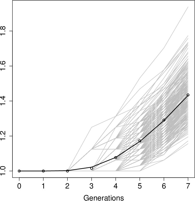
On the other hand, for $\gamma=0$, Proposition 1-b gives a much faster decay of the tail distribution

$\displaystyle P(T>t)$

$\displaystyle\sim\pi_{t}R(1)^{l^{t}}=p_{l}^{-\frac{1}{l-1}}\rho^{l^{t}},\quad t\to\infty,$

(8)

where $\rho=p_{l}^{\frac{1}{l-1}}R(1)\in(0,1)$. This yields $P(T=t|T\geq t)\to 1$. The next Theorem 3 establishes a conditional weak law of large numbers for ${l}^{t-k}Z(t-k)$.

According to Theorem 3-b, if $f^{\prime\prime}(1)<\infty$, then conditionally on $T>t$, we have convergence in probability $Y(t-k)\to c(k)$ as $k\geq 0$ is fixed and $t\to\infty$, and convergence in probability $Y(k)\to 1$ as $t-k\to\infty$. This indicates that being conditioned on survival, the reproduction regime prefers the minimal offspring number ${l}$, especially at early times (see Figure 1).

Suppose $f(r)=r$ for some $r>1$, so that necessarily $f(1)<1$ (see Figure 2). In this case the corresponding defective GW-process $Z(\cdot)$ could be called an extendable GW process because the usual range $0\leq s\leq 1$ for the reproduction generating function $f(s)$ can be extended to $0\leq s\leq r$. The transformed function

$$\hat{f}(s)=r^{-1}f(rs),\quad s\in[0,1],\quad\hat{f}(1)=1,$$

generates a proper reproduction distribution $\hat{p}_{k}=r^{k-1}p_{k}$ with mean $\hat{m}=\hat{f}^{\prime}(1)=f^{\prime}(r)$. Denote by $\hat{Z}(\cdot)$ the GW-process with the reproduction law $\hat{f}(\cdot)$. If $\hat{m}\in(1,\infty)$, then by Theorem 3 in [2, Ch I.10], there exists a sequence $C(t)\to\infty$, $t\to\infty$ such that $\hat{Z}(t)/C(t)\to W$ a.s., where $P(W>0)=1-\hat{q}$ and $\hat{q}=q/r$. In this case, for any given $\lambda\geq 0$, we have a positive finite limit

$$E(e^{-\lambda\hat{Z}_{n}(t)/C(t)}|\hat{T}_{0}>t)\to\Psi(\lambda),\quad t\to\infty,$$

(10)

where $\Psi(\lambda)=E(e^{-\lambda W}|W>0)$. On the other hand, if $\hat{m}=\infty$, then by [4],

$$P(b^{-t}\ln\hat{Z}(t)\leq u|\hat{T}_{0}>t)\to\psi(u),\quad u\in(0,\infty),$$

(11)

provided the following condition holds

$$g^{\prime}(x)=ax^{b-1}(1+O(x^{\delta})),\quad x\to 0,\quad a>0,\quad b>1,\quad\delta>0.$$

Here $g(\cdot)=G_{-1}(\cdot)$ is the inverse function of $G(x)=1-f(1-x)$, and the limit $\psi(\cdot)$ in (11) is continuous and strictly monotonic increasing function such that

$$\psi(u)\to 0,\quad u\to 0+,\qquad\psi(u)\to 1,\quad u\to\infty.$$

Theorem 4-a should be compared to [7, Theorem 3.4] concerning a sequence of GW-processes with killing: if $Z_{n}(\cdot)$ has a reproduction law of the form $f_{n}(s)=\hat{f}(\alpha_{n}s)$, where $\hat{f}(1)=1$, $\hat{f}^{\prime}(1)\in(1,\infty)$, and

$$(1-\alpha_{n})C(t_{n})\to(\hat{m}-1)x/\hat{m},\quad n\to\infty,$$

then the same weak convergence result (13) holds. The proof of Theorem 4 given in Section 6 is more straightforward than the proof of [7, Theorem 3.4], which demonstrates the advantage of dealing with the extendable GW-processes.

The main assumption of Section 3 is quite restrictive on the mode of convergence $f_{n}(\cdot)\to\hat{f}(\cdot)$, namely, condition (12) requires that the sequence $f_{n}(\cdot)$ has a common shape of the reproduction laws and only a scale parameter $r_{n}\to 1$ is changing as $n\to\infty$. In this section we take a step towards a more general setting for the convergence $f_{n}(\cdot)\to\hat{f}(\cdot)$. We focus on the parametric family of the theta-branching processes introduced in [9]. Our Propositions 5, 6 and 7 give explicit expressions for the corresponding limit distributions.

Proposition 5 is a counterpart of Theorem 4-a in terms of a sequence of extendable GW-processes whose generating functions are explicitly characterized by four parameters

$$(\theta_{n},q_{n},\gamma_{n},r_{n})\in(0,1]\times[0,1)\times(0,1)\times(1,\infty)$$

as follows

$\displaystyle f_{n}(t,s)=r_{n}-\left[\gamma_{n}^{t}(r_{n}-s)^{-\theta_{n}}+(1-\gamma_{n}^{t})(r_{n}-q_{n})^{-\theta_{n}}\right]^{-1/\theta_{n}},\quad s\in[0,r_{n}],$

In agreement with our previous notation, $q_{n}$ is the extinction probability and $\gamma_{n}=f_{n}^{\prime}(q_{n})$. These are defective GW-processes with the defect value

$$\varepsilon_{n}=\left[\gamma_{n}(r_{n}-1)^{-\theta_{n}}+(1-\gamma_{n})(r_{n}-q_{n})^{-\theta_{n}}\right]^{-1/\theta_{n}}-(r_{n}-1).$$

Under the conditions of Proposition 5 we have $f_{n}(s)\to\hat{f}(s)$, where

$\displaystyle\hat{f}(s)=1-\left[\gamma(1-s)^{-\theta}+(1-\gamma)(1-q)^{-\theta}\right]^{-1/\theta}.$

(16)

For the corresponding supercritical GW-process having the offspring mean $\hat{m}=\gamma^{-1/\theta}$, it is straightforward to check that the limit Laplace transform

$$E(e^{-\lambda\hat{Z}(t)\hat{m}^{-t}}|\hat{T}_{0}>t)=1-{1-\hat{f}(t,e^{-\lambda\gamma^{t/\theta}})\over 1-\hat{f}(t,0)}\to\Psi(\lambda),\quad t\to\infty,$$

is given by (15). Since

$$\varepsilon_{n}\sim(\gamma^{-1/\theta}-1)(r_{n}-1),\quad n\to\infty,$$

the first part of Proposition 5 essentially says that for a given small $\varepsilon$, the absorption time $T$ of a defective theta-branching process with $\theta\in(0,1]$ is of order $\theta\log_{\gamma}\varepsilon$. Observe that the new normalization $m_{n}^{t_{n}}$ may not be asymptotically equivalent to the normalization $\hat{m}^{t_{n}}$ suggested by Theorem 4-a under an additional ”xlogx” condition.

The next two propositions deal with two different sequences $f_{n}(\cdot)$ converging to the same limit reproduction law given by

$\displaystyle\hat{f}(s)=1-(1-q)^{1-\gamma}(1-s)^{\gamma},\quad s\in[0,1],$

(17)

with $q\in[0,1)$, $\gamma\in(0,1)$, $\hat{f}(1)=1$, and $\hat{m}=\hat{f}^{\prime}(1)=\infty$. Plugging $s=\exp\{-\lambda e^{-u\gamma^{-t}}\}$ into

$$\hat{f}(t,s)=1-(1-q)^{1-\gamma^{t}}(1-s)^{\gamma^{t}},$$

it is straightforward to find a convergence

$\displaystyle P\left(\gamma^{t}\ln\hat{Z}(t)\leq u|\hat{T}_{0}>t\right)\to 1-e^{-u},\quad u\geq 0$

to a standard exponential distribution.

Since in this parametric case the defect size has the asymptotic value

$$\varepsilon_{n}\sim(1-q)^{1-\gamma}(r_{n}-1)^{\gamma},\quad n\to\infty,$$

the first part of Proposition 6 essentially says that for a given small defect value $\varepsilon$, the absorption time of a defective theta-branching process with $\theta\in(0,1]$ is of order $\ln\ln\varepsilon^{-1}$.

Here, $\varepsilon_{n}\sim(1-q)(1-\gamma)^{1/|\theta_{n}|}$ and by Proposition 7-a, given a small defect value $\varepsilon$, the absorption time is again of order $\ln\ln\varepsilon^{-1}$. If $A_{n}\equiv 1$, then $a=\infty$, and convergence in Proposition 7-a is given by (20). To see a connection of the convergence in Proposition 7-b₁ to that of Proposition 7-b₂, notice that $\hat{u}(x)\to u$, as $x\to\infty$.

References

- [1] K. B. Athreya. Large deviation rates for branching processes–I single type case. The Annals of Applied Probability, 1994, 4(3), 779–790.
- [2] K.B. Athreya and P.E. Ney. Branching processes. Springer, 1972.
- [3] P. Braunsteins, and S. Hautphenne, On the extinction of Lower Hessenberg branching processes with countably many types. Work in progress, 2017.
- [4] D.A. Darling. The Galton-Watson process with infinite mean. Journal of Applied Probability, 1970, 7(2), 455–456.
- [5] S. Karlin and S. Tavaré. Detecting particular genotypes in populations under nonrandom mating. Mathematical Biosciences, 1982, 59(1), 57–75.
- [6] S. Méléard. Quasi-stationary distributions and population processes. Probability Surveys, 2012, 9, 340–410.
- [7] A.G. Pakes. The Galton-Watson process with killing. Mathematical Biosciences, 1984, 69(2), 171–188.
- [8] S. Sagitov. Tail generating functions for extendable branching processes. Stochastic Processes and their Applications, 2017, (in press).
- [9] S. Sagitov and A. Lindo. A special family of Galton-Watson processes with explosions. In Branching Processes and Their Applications, volume 219 of Lecture Notes in Statistics - Proceedings, I.M. del Puerto, M. González, C. Gutiérrez, R. Martínez, C. Minuesa, M. Molina, M. Mota, and A. Ramos, Eds.; Springer, 2016; 237–254.
- [10] S. Sagitov and M. Serra. Multitype Bienaymé-Galton–Watson processes escaping extinction. Advances in Applied Probability, 2009, 41(1), 225–246.
- [11] N. M. Yanev. Conditions for degeneracy of -branching processes with random . Theory of Probability and its Applications, 1975, 20, 421–428.