On kernel design for regularized LTI system identificationfootnoteinfo
Abstract
There are two key issues for the kernel-based regularization method: one is how to design a suitable kernel to embed in the kernel the prior knowledge of the LTI system to be identified, and the other one is how to tune the kernel such that the resulting regularized impulse response estimator can achieve a good bias-variance tradeoff. In this paper, we focus on the issue of kernel design. Depending on the type of the prior knowledge, we propose two methods to design kernels: one is from a machine learning perspective and the other one is from a system theory perspective. We also provide analysis results for both methods, which not only enhances our understanding for the existing kernels but also directs the design of new kernels.
keywords
System identification, regularization methods, kernel methods, kernel design, prior knowledge.footnoteinfo]Abridged and preliminary results of this paper was presented in the 19th
IFAC World Congress, Cape Town, South Africa, 2014, the European Research Network on System Identification (ERNSI) workshop, Ostend, Belgium,
2014, and the 17th IFAC Symposium on System Identification, Beijing, China, 2015.
This work is supported by the Thousand Youth Talents Plan funded by
the central government of China, the Shenzhen Projects Ji-20170189 and Ji-20160207 funded by Shenzhen Science and Technology Innovation Council,
the President’s grant under contract No. PF. 01.000249 and the
Start-up grant under contract No. 2014.0003.23 funded by the Chinese
University of Hong Kong, Shenzhen, as well as by a research grant
for junior researchers under contract No. 2014-5894, funded by
Swedish Research Council.
1 Introduction
Among diverse system identification problems, the linear time-invariant (LTI) system identification is a classical and fundamental problem. As well-known, an LTI system is uniquely characterized by its impulse response, and thus the LTI system identification is equivalent to its impulse response estimation that could be ill-conditioned in practice. So to tackle the LTI system identification, one needs to first find a way to make the ill-conditioned problem well-conditioned. Then one faces the core issue of system identification, i.e., how to construct a model estimator able to achieve a good bias-variance tradeoff, or equivalently, to suitably balance the adherence to the data and the model complexity.
There are different routes to handle these two issues. The most widely used route is to adopt instead a parametric model structure with a finite number of parameters. The so-called maximum likelihood/prediction error method (ML/PEM) is one method along this route. It has optimal asymptotic properties and is the current standard method to LTI system identification. It first postulates a parametric model structure, e.g., a rational transfer function, then forms the prediction error criterion, and finally obtains the model estimator by minimizing the prediction error criterion; see e.g., [1, 2]. The model complexity of the parametric model structure is governed by the number of parameters and tuned in a discrete manner. The bias-variance tradeoff issue is handled by cross validation or model structure selection criteria such as Akaike’s information criterion (AIC), Bayesian information criterion (BIC), and etc, which correspond to combinatorial optimization problems; see e.g., [1, Chapter 16]. However, these techniques are not as reliable as expected when the data is short and/or has low signal-to-noise ratio; see e.g., [3, 4].
Another route is to adopt regularization by adding an extra regularization term in the estimation criterion. The kernel-based regularization method (KRM) proposed in the seminal paper [5] and further developed in [6, 3, 7] is one method along this route. It first proposes a kernel parameterized by some hyper-parameters for the impulse response, then estimates these hyper-parameters with certain methods, and finally obtains the estimate of the impulse response by minimizing a regularized least squares criterion with the regularization term in quadratic form and the regularization matrix defined through the kernel; see [4] for a recent survey. While the impulse response model is used, the underlying model structure is determined by the kernel. The model complexity is governed by the hyper-parameters of the kernel, and tuned in a continuous manner by e.g., the empirical Bayes method, Stein’s unbiased risk estimator [4, 8, 9] and etc., which correspond to non-convex but non-combinatorial optimization problems.
The route to adopt regularization is by no means new, see e.g., [10], [11], [1, p. 504-505] and also [12] for a historic review, but no important progress along this route has been reported until [5]. The major obstacle is that it was unclear whether or not it is possible to design the regularization to embed the prior knowledge of the LTI system to be identified. The intriguing finding disclosed by the KRM is that when considering impulse response estimation problem, it is possible to design a regularization in quadratic form or equivalently a kernel to embed the prior knowledge of the impulse response of the LTI system to be identified. So far several kernels have been invented to embed various prior knowledge, e.g., [5, 6, 3, 7, 13, 14, 15, 16, 17, 18, 19] and some analysis results of the corresponding kernels have been derived, e.g., [5, 3, 7, 13, 14, 15, 16, 17, 18]. Still, there lack systematic ways to design kernels to embed in the kernel the prior knowledge of the impulse response of the LTI system to be identified.
In this paper, we try to develop systematic ways to design kernels. Clearly, this issue relates to the type of the prior knowledge. Interestingly, even for the same impulse response estimation problem, users with different background may come up with different types of prior knowledge because they may treat the impulse response in different ways. For instance, users from machine learning may treat the impulse response as a function, whose amplitude varies with a certain rate and decays exponentially to zero in the end; users from signals and systems may associate the impulse response with an LTI system that is stable and may be overdamped, underdamped, has multiple distinct time constants and resonant frequencies, and etc. Accordingly, we provide two methods to design kernels to embed the corresponding type of prior knowledge from a machine learning perspective and from a system theory perspective, respectively.
To develop the machine learning method, we first point out a common feature of the two most widely used single kernels, i.e., the stable spline (SS) kernel in [5] and the diagonal-correlated (DC) kernel in [3], that they belong to the class of the so-called amplitude modulated locally stationary (AMLS) kernel. The AMLS kernel is a multiplication of two kernels: a rank-1 kernel and a stationary kernel. It has a neat implication: the zero mean Gaussian process with the AMLS kernel as the covariance function can be seen as an amplitude modulated (by the rank-1 kernel) zero mean Gaussian processes with the stationary kernel as covariance function; see Section 3 for details. This finding leads to the machine learning method to design general kernels: design the rank-1 kernel and the stationary kernel to account for the decay and the varying rate of the impulse response, respectively.
To develop the system theory method, we recall the general guideline to design a kernel in [3] that is to let the kernel mimic the behavior of the optimal kernel [3, Thm. 1] and [4, Prop. 19]. Moreover, the prior knowledge for the impulse response, or equivalently, the LTI system to be identified, shall be made use of, since the optimal kernel depends on the true impulse response. Following this guideline and employing the multiplicative uncertainty configuration in robust control, see e.g. [20], we design the simulation induced (SI) kernel. In particular, the prior knowledge is embedded in the nominal model, the uncertainty is assumed to be stable and finally, the multiplicative uncertainty configuration is used to take into account both the nominal model and the uncertainty and is simulated with an impulsive input to get the SI kernel. Then we make analysis for SI kernels in terms of stability, maximum entropy property, and Markov property, with the SS and DC kernels as examples. In particular, we give conditions under which the SI kernel is stable, solves a suitably defined entropy maximization problem, and induces a Gaussian Markov process. The maximum entropy interpretation enhances our understanding about a kernel, and the Markov property of a kernel ensures that the inverse of the kernel matrix is banded and this special structure can be exploited to derive more stable and efficient implementation for the KRM, see e.g., [21, 18].
The remaining part of this paper is organized as follows. In Section 2, the KRM is recapped. The machine learning and system theory methods to design kernels are introduced in Section 3 and 4, respectively. Then a case study is provided in Section 5 to demonstrate how to design kernels from the proposed two methods to model impulse responses with damped oscillation. Finally, this paper is concluded in Section 6 with a take-home message. The proofs of all propositions and theorems are given in the Appendix.
2 LTI System Identification with Kernel-based Regularization Method
2.1 Impulse Response Estimation
Consider a single-input-single-output, causal and LTI system described by
| (1) |
where is the time index, and are the measured output, input, disturbance, and impulse response of the LTI system at time , respectively, is the convolution between the impulse response and the input evaluated at time , and is the sampling period and for convenience chosen to be 1.
The system (1) represents both discrete-time (DT) system with and continuous-time system (CT) with . In particular, we have
where the unmeasured portions of are set to zero. Moreover, the system (1) is assumed to be stable, i.e., for the DT case and for the CT case, where denotes the space of absolutely convergent sequences and denotes the space of absolutely Lebesgue integrable functions on , and the disturbance is assumed to be a white Gaussian noise with zero mean and variance and independent of .
The goal of LTI system identification is to estimate the impulse response as well as possible given the data with for the DT case and with and with for the CT case.
2.2 Kernel-based Regularization Method
As well-known [10], [1, p. 504-505], straightforward impulse response estimation, i.e.,
could be an ill-conditioned problem in practice and one way to overcome this problem is to adopt regularization. Moreover, the recent progresses for KRM [5, 6, 3, 7] show that if the regularization is well designed and tuned, the resulting regularized impulse response estimator can also achieve a good bias-variance tradeoff.
To introduce the KRM, we first recall the definition of the positive semidefinite kernel and its associated reproducing kernel Hilbert space (RKHS). Let be a metric space with being its metric. A function is called a positive semidefinite kernel, if it is symmetric and satisfies for any finite set of points and . As well-known from e.g., [22], to every positive semidefinite kernel there corresponds to one and only one class of functions with a unique determined inner product in it, leading to the so-called reproducing kernel Hilbert space (RKHS) with as the reproducing kernel.
The KRM first introduces a suitable positive semidefinite kernel 11 1 Sometimes the dependence of on is ignored.with , where for the DT case, and for the CT case, , and is a hyper-parameter vector that contains the parameters used to parameterize the kernel, and then solves the following regularized least squares problem:
| (4) |
where is the norm of in , and is a regularization parameter and controls the tradeoff between the data fit and the regularization term .
We will discuss the issue of kernels in the next subsections. For the time being, we assume that a suitable kernel has been designed, but its hyper-parameter is left to be determined. The current most widely used method to determine is the so-called empirical Bayes method [23]. It first embeds the regularization in a Bayesian framework, and then estimates and possibly also the noise variance by maximizing the marginal likelihood , where with being its th element, and could be or the concatenation of and . Specifically, we define with its th element defined by
and moreover, we let , where is the -dimensional identity matrix. Then we get
where is a constraint set where we search for . When an estimate of is obtained, the solution to (4) is given by the representer theorem [4, Theorem 3]:
| (5) |
where is the th element of .
2.3 Existing Single Kernels
So far the two mostly widely used single kernels are the stable spline (SS) kernel [5] and the diagonal/correlated (DC) kernel [3]. The SS kernel is defined as
| (6) |
and the DC kernel is defined as
| (7) | ||||
| (8) | ||||
where the TC kernel is a special case of the DC kernel with and is also called the first order stable spline kernel.
Remark 2.1
It is worth to note that for and , is complex and thus with is not well defined for the CT case.
2.4 Optimal Kernel and Stable Kernel
For the KRM, the optimal kernel in the sense of minimizing the mean square error (MSE) exists [3, 4] and motivates a general guideline to design a kernel. To state this result, we assume that the data has been generated by (1) for a true impulse response and we let and to represent any finite dimensional vector obtained by sampling and its estimate at the same arbitrary time instants. Then the following result holds.
Lemma 2.1 (Optimal kernel, [3, 4])
Letting . Then for the KRM, the MSE matrix
| (11) |
where is the mathematical expectation, is minimized by the kernel
| (12) |
in the sense that is positive semidefinite for any positive semidefinite kernel .
The optimal kernel cannot be applied in practice as it depends on the true impulse response . However, it motivates a general guideline to design a kernel: let the kernel mimic the behavior of the optimal kernel, and moreover, the prior knowledge of the true impulse response should be used in the design of the kernel.
For instance, if the LTI system is known to be stable, i.e., or , then the designed kernel should reflect this, and a necessary condition to satisfy is that should tend to 0 as goes to infinity. This observation basically rules out the possibility to model the impulse response of stable LTI systems with stationary kernels22 2 Recall that a kernel with is said to be stationary if is a function of for any . and a rigorous proof for this has been given in [13, Lemma 8]. More generally, the designed kernel should guarantee that its associated RKHS is a subspace of or and a kernel that has such property is said to be stable [13, 4]. Sufficient and necessary conditions for a kernel to be stable exist and are given below.
2.5 Kernel Design
Hereafter, we focus on the problem of kernel design. The problem is stated as follows: for the given prior knowledge of the impulse response to be identified, our goal is to design a kernel such that the prior knowledge is embedded in the kernel. The answer should depend on the type of the prior knowledge. We will consider two types of prior knowledge and discuss how to design kernels accordingly from two perspectives: a machine learning perspective and a system theory perspective.
It should be noted that the LTI system (1) is assumed to be stable, meaning that or becomes our first prior knowledge. In this regard, Theorem 2.2 becomes a rule that the designed kernel should obey.
Remark 2.2
Other than stability, the cases where the impulse response or the corresponding LTI system is known to have relative degree, to be monotonic, smooth and to have delay, have been discussed in [13] and in particular, sufficient and/or necessary conditions for a kernel to have such properties are given. For instance, if a CT kernel is -times continuously differentiable, then every function is -times continuously differentiable [25, Corollary 4.36, p. 131], [13, Lemma 5].
3 A Machine Learning Perspective
We first show that both the SS kernel and the DC kernel belong to the class of the so-called amplitude modulated locally stationary (AMLS) kernel. Accordingly, we propose to treat the impulse response as a function, whose amplitude varies with a certain rate and decays exponentially to zero in the end, and moreover, design AMLS kernels to model the impulse response.
3.1 Amplitude Modulated Locally Stationary Kernels
Recall that a kernel is said to be a locally stationary (LS) kernel in the sense of Silverman [26] if
| (17) |
where and is a stationary kernel33 3 Clearly, if is a positive constant, then the LS kernel reduces to a stationary kernel. . Motivated by the LS kernel, we introduce a kernel suitable for modeling impulse response, which is called the amplitude modulated locally stationary (AMLS) kernel.
Definition 3.1
A kernel is said to be an amplitude modulated locally stationary kernel if
| (18) | ||||
where is bounded and is a stationary kernel.
It can be proved that the AMLS kernels have the following properties (proof given in the Appendix).
Proposition 3.1
Consider the AMLS kernel (18). Then the following results hold:
- (a)
is a rank-1 kernel44 4 A kernel with is said to be a rank-1 kernel if for any , and for any , the kernel matrix , defined by , is a rank-1 matrix. and moreover satisfy
(19) - (b)
Let be a stochastic process with zero mean and the AMLS kernel as the covariance function. Then is the correlation coefficient between and .
- (c)
Let be a stochastic process with zero mean and as the covariance function. Then the stochastic process has zero mean and the AMLS kernel as its covariance function.
Remark 3.1
Since is the correlation coefficient and , then is bounded and moreover, for any .
For a function estimation problem, if a zero mean Gaussian processes with the AMLS kernel as the covariance function is chosen to model the function, then Proposition 3.1 has the following implications:
- •
The stationary kernel in (18) accounts for the varying rate of the function.
Note that part (b) shows that is the correlation coefficient for , which implies that
The above equation shows that for any fixed , as varies from 1 to , tends to become larger, that is, tends to vary more quickly away from . This observation also holds for as is also the correlation coefficient for .
- •
The rank-1 kernel in (18) account for the change of the amplitude of the function.
Note that part (c) shows that the amplitude of is modulated by the factor . If does not converge to 0 as goes to , then a suitable can be chosen such that does.
Interestingly, both the SS and DC kernels can be put in the form of (18). Setting and using the equality yields that the SS kernel (6) is rewritten as
| (20) |
Then we identify, for the SS kernel (20),
| (21) |
and for the DC kernel (7),
| (22) |
Moreover, one can prove the following result (proof given in the Appendix).

Now we demonstrate for the SS and DC kernels the role of the rank-1 kernel and the stationary kernel .
Example 3.1
As seen from the left panel of Fig. 1, as changes from to , the realizations of the DT zero mean Gaussian process with in (21) as the covariance function varies more quickly, because . Similarly, as changes from , to and to , the realizations of the DT zero mean Gaussian process with in (22) varies more quickly, and especially for the case with , the realization tends to change its sign at the next time instant. The above observations carry over to the right panel of Fig. 1. Finally, the realizations on the left panel of Fig. 1 do not go to zero for large but the realizations on the right panel do, because of .
3.2 Construct AMLS Kernels for Regularized Impulse Response Estimation
Proposition 3.2 and its implications on the role of the rank-1 kernel and the stationary kernel suggest a machine learning method to design kernels for regularized impulse response estimation. If the impulse response is treated as a function and the prior knowledge is about its decay and varying rate, then AMLS kernels can be designed by choosing suitable rank-1 kernel and stationary kernel to account for the decay and varying rate of the impulse response, respectively.
3.2.1 Stationary Kernel
An important class of stationary kernels is the isotropic stationary (IS) kernel. Recall that a stationary kernel is said to be an IS kernel if it depends on . IS kernels have been studied extensively in the literature in statistics and machine learning, see e.g. [27, Section 4.2.1]. There are many choices of IS kernels that could be used instead of the ones in (21) and (22).
Most of the IS kernels introduced in [27, pages 83 -88] decay monotonically w.r.t. and are always positive. For example, the squared exponential (SE) kernel and the Matèrn class of kernels:
where , is the Gamma function and is a modified Bessel function with order .
There are IS kernels that do not decay monotonically, can take negative values, and can have the form of damped oscillation w.r.t. . For example, the kernel in [27, p. 89], [28]:
| (23a) | ||||
| where , is a scalar such that , and is the Bessel function of the first kind with order . The kernel (23a) is defined for any and can thus be used for both CT and DT impulse response estimation. In particular, for and , the kernel (23a) takes the following form | ||||
| (23b) | ||||
| (23c) | ||||
3.2.2 Rank-1 Kernel
The design of is equivalent to that of the strictly positive function in (18). The bottom line is that should ensure that the designed AMLS kernel (18) is stable, i.e, is a subspace of or . Our following result gives a characterization of the stability of the AMLS kernel (proof given in the Appendix).
Proposition 3.3
Consider the AMLS kernel (18). Then the following results hold.
- (a)
If for the DT case, and for the CT case, then the AMLS kernel (18) is stable.
- (b)
Assume that there exists a sequence of positive numbers and linearly independent functions defined on such that
(24) where the convergence is absolute and uniform on with being any compact subsets of . If the AMLS kernel (18) is stable, then there exists no such that for all .
Since the in (21) and (22) are exponential decay functions and clearly satisfy or , the SS and DC kernels are stable by Proposition 3.3.
Remark 3.3
It is reasonable to check wether the condition (24) is too strong to be satisfied. In fact, the series expansion (24) can be obtained by Mercer’s Theorem [29, 30, 31]. For instance, a sufficient condition for (24) to hold is given in [31]. To state this result, we define the kernel section of at a fixed as and we let denote the space of functions such that , where is a nondegenerate Boreal measure on . Then (24) holds if is continuous, and
| (25) |
It is easy to check that many stationary kernels satisfy the above sufficient condition, e.g., the SE kernel and the in (21) and (22).
Remark 3.4
It follows from (71) that if there exists an such that for all , then , implying that is also necessary for the stability of the AMLS kernel (18). The above observations show that under the assumption that the AMLS kernel (18) is stable, the result we can draw on the properties of is determined by the property of .
Remark 3.5
The reason why we force for is because for a kernel in the form of , we expect the two kernels and have somewhat independent role. As shown above, this idea eases the kernel design and the corresponding analysis. If this idea is not taken, then we can design more general and even more general . For instance, we could allow to be arbitrary real-valued function and we could also allow to be the more general exponentially convex (EC) kernel55 5 For the LS kernel (17), if is also a kernel, then is called an exponentially convex (EC) kernel [32] and in this case is called an exponentially convex locally stationary (ECLS) kernel [26]. and design accordingly the ECLS kernel [15] instead of the AMLS kernel. The price to pay is that the role of and would become obscure and in particular, would not describe the decay rate and would not be the correlation coefficient of the underlying Gaussian process.
4 A System Theory Perspective
Instead of simply treating the impulse response as a function, we now associate the impulse response with an LTI system which is stable and may be overdamped, underdamped, have multiple distinct time constants and resonant frequencies, and etc., and our goal is to design kernels to embed this kind of prior knowledge.
4.1 Sketch of The idea
Suppose that the prior knowledge of an LTI system is embedded in a stochastic process that is used to model the corresponding impulse response. Then following the guideline to design kernels in Section 2.4 that is to mimic the behavior of the optimal kernel (12), we should design the kernel as
| (26) |
where is the covariance between and . Now the problem of kernel design becomes “how to embed the prior knowledge of an LTI system in a stochastic process that is used to model the corresponding impulse response”?

A natural way to tackle the above question is by using simulation. To this goal, it is useful to employ the multiplicative uncertainty configuration in robust control, see e.g., [20], as shown in Fig. 2. Here, the nominal model is used to embed the prior knowledge on the LTI system to be identified, the uncertainty is assumed to be stable and finally, the multiplicative uncertainty configuration is used to take into account both the nominal model and the uncertainty, and is simulated with an impulsive input to get a zero-mean Gaussian process to model the impulse response . This idea leads to the system theory method to design kernels and we call such kernels the simulation induced (SI) kernels.
Remark 4.1
It is worth to note that the problem of marrying system identification and robust control is not new and has been studied over two decades in the system identification community, see e.g., [33, 34]. Both the additive uncertainty configuration and the multiplicative uncertainty configuration have been used and many results have been obtained, see e.g., [35, 33, 34, 36, 37, 38]. In particular, [35, 33, 36, 37, 38] used the nominal model and the uncertainty to represent a model estimate and the corresponding model error, respectively. Here the nominal model and the uncertainty are used to embed the prior knowledge of the LTI system and describe the corresponding uncertainty, respectively.
4.2 Simulation Induced Kernel
More specifically, the prior knowledge is embedded in or equivalently, in its state-space model
| (27a) | |||||
| (27b) | |||||
| (27c) | |||||
| (27d) | |||||
where , and have compatible dimensions, and are the input and output of , respectively. In what follows, we will use the quintuple to represent the state-space model (27).
Since the uncertainty is stable, the simplest way to model the impulse response of with a stochastic process , is to have
| (28) |
where is a white Gaussian noise with zero mean and unit variance (independent of ), and and or for the DT and CT case, respectively. Clearly, is a zero mean Gaussian process with the AMLS kernel as the covariance function, where is the Dirac Delta function and the AMLS kernel is stable by Proposition 3.3.
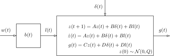
Finally, we simulate the system in Fig. 2 with the impulsive input and noting (27), (28) and , we obtain the simulation induced (SI) kernel:
| (29a) | ||||
| (29b) | ||||
| (29c) | ||||
| (29d) | ||||
| (29e) | ||||
whose block diagram is shown in Fig. 3. From linear system theory, e.g., [39], the formal expression of the SI kernel (29) is available. For the DT case, it is
| (30a) | ||||
| For the CT case with , it is | ||||
| (30b) | ||||
Remark 4.2
It should be noted that both DT and CT cases are considered in (27) and (29). For the CT case, (29b) could be more rigorously written as an Itô stochastic differential equation (SDE) as in [14, eq. (9)]. However, we decide to take the same point of view as in [40] to use (29b) instead in order to save the space for the introduction of SDE stuff, which is only used to derive (30b).
Remark 4.3
The SI kernels (30) may or may not have closed form expressions. The related computational difficulty and cost depend on whether or not the SI kernels (30) have closed form expressions. If they do, then the computation would be easier and similar to the SS and DC kernels. If they do not, the computation of the hyper-parameter estimate and the regularized impulse response estimate would become more demanding. In this regard, the particle filtering based technique for nonlinear state-space model identification in [41] could be adopted. However, the technique in [41] cannot be applied trivially as the measurement output (1) for the state space model (29) does not depend on the current state solely but also the past state due to the presence of convolution. More details will be reported in an independent paper.
Note that in (29) is a Gaussian process with the impulse response of the LTI system as its mean and the SI kernel as its covariance function. If is set to 0 in (29), in (29) is a zero mean Gaussian process with the SI kernel as its covariance function. In what follows, when considering kernel design, we will set to zero for convenience.
Interestingly, the AMLS kernel (18) is closely related with the SI kernel (29), and in fact many AMLS kernels such as the SS and DC kernels can be put in the form of (29) and are thus SI kernels. To state this result, recall that the power spectral density of , denoted by , is defined as
Proposition 4.1
Proposition 4.2
Proposition 4.2 enhances our understanding about the SS and DC kernels and in particular, the prior knowledge embedded in the two kernels from a system theory perspective is as follows:
- 1)
For the SS kernel, the corresponding nominal model in Fig. 2 is a second order system. For the DC kernel, the corresponding nominal model is a first order system. For both the SS and DC kernels and for the CT case, has negative real poles corresponding to overdamped impulse responses. For the DT case, the two poles for the SS kernel are real positive and correspond to impulse response without oscillation, and the pole for the DC kernel can be positive or negative (depending on ) and corresponds to impulse response without or with oscillation. The pole for the TC kernel is positive (equal to ) and corresponds to impulse response without oscillation.
- 2)
For both the SS and DC kernels, the decay rate of the impulse response of the uncertainty in Fig. 2 are all described by exponential decay functions.
Remark 4.4
It is worth to note that to study the link between a kernel and its state-space model realization has a long history, see e.g., [42, 40]. This link is important because it opens the body of a kernel from a system theory perspective and accordingly helps to understand the underlying behavior of a kernel.
4.3 Stability of SI kernels
For the SI kernel (30), we provide the following sufficient condition to guarantee its stability.
Proposition 4.3
Consider the SI kernel (30).
- •
For the DT case, assume that has distinct eigenvalues and moreover, is stable, i.e., has all eigenvalues strictly inside the unit circle. Assume further that
(50a) for some , where is the eigenvalue of with the largest modulus. Then the SI kernel (30a) is stable.
- •
For the CT case, assume that has distinct eigenvalues and moreover is stable, i.e., has all eigenvalues with strictly negative real parts. Assume further that
(50b) for some , where is the eigenvalue of with the largest real part and is the real part of . Then the SI kernel (30b) is stable.
Remark 4.5
The conditions (50) are sufficient but not necessary. For instance, consider the DT case. The SS kernel (• ‣ 4.2) satisfies (50a) but the DC kernel (41) does not. It is possible to derive a slower upper bound for . Another intension to have Proposition 4.3 is to give some guidelines about the relations between , and the stability of SI kernel: in order to guarantee stability of the SI kernel, the impulse response of the uncertainty (28), i.e., should decay a bit faster than the slowest mode of the nominal model .
4.4 Maximum Entropy Property of SI Kernels
Since the prior knowledge is never complete, it is worth to note Jaynes’s maximum entropy (MaxEnt) rationale [43] to derive from incomplete prior knowledge the optimal statistical prior distribution. Jaynes’s idea is to formulate a MaxEnt problem with respect to the prior, and then solve the problem to obtain the optimal prior. The constraints of the problem describes the prior knowledge (in the MaxEnt sense) of the underlying stochastic process (the system) to be identified. Interestingly, the SI kernel lends itself easily to a MaxEnt interpretation, leading to a new facet to understand the underlying behavior of the SI kernel.
Recall that the differential entropy of a real-valued continuous random variable is defined as , where is the probability density function of and is the support set of . Then we prove the next MaxEnt interpretation of SI kernels66 6 Let be two jointly distributed random variables. Then the joint differential entropy of is simply written as below. .
Proposition 4.4
Consider the SI kernel (29) with (30a).
- •
For the case , define
(51) Then for any , the Gaussian process in (29) is the solution to the MaxEnt problem
(52a) subject to (52b) where is the covariance matrix of and is the variance of . - •
For the case , assume that and define
(53) Then for any , the Gaussian process in (29) is the solution to the MaxEnt problem
(54a) subject to (54b)
Corollary 4.1
For any , the zero mean Gaussian process with the DC kernel (7) defined on as its covariance is the solution to the MaxEnt problem
| (55) | ||||
Remark 4.6
When , the DC kernel (7) becomes the TC kernel (8). For the TC kernel defined on , (55) becomes
| (56) | ||||
which is different from the MaxEnt interpretation in [17]. It shall be noted that both interpretation are correct but derived in different ways: the MaxEnt problems are different but have the same optimal solution.
Remark 4.7
Remark 4.8
The CT case is not discussed here because according to our best knowledge the entropy is not well defined for CT stochastic processes.
4.5 Markov Property of SI Kernels
As shown in [44, 19, 18, 17], the kernel matrix of DC kernel (7) has tridiagonal inverse. Here, we further show that the Gaussian process with the DC kernel as its covariance function is also a Markov process with order 1 and moreover, we are able to design SI kernels which correspond to more general Gaussian Markov processes and have banded77 7 A real symmetric matrix with dimension is called an band matrix if for .inverses of their kernel matrices.
First, recall from e.g., [27, Appendix B] that a Gaussian Markov process is a stochastic process that is both a Gaussian process and a Markov process. A well-known instance is the DT autoregressive process of order :
| (57a) | ||||
| (57b) | ||||
where , , is Gaussian distributed and assumed to be independent of , a zero mean white Gaussian noise with unit variance. The stochastic process (57) is a Markov process with order since only depends on given the history with .
Proposition 4.5
Consider a zero mean DT Gaussian process with the DC kernel (7) as its covariance. Then with can be put in the form of
| (58) |
and thus a Markov process with order 1, and moreover, its kernel matrix has a -band matrix inverse.
Remark 4.9
It is possible to construct more general SI kernels with Markov property.
Proposition 4.6
For illustration, we consider an example.
Example 4.1

Remark 4.10
The Markov property of a kernel and its associated special structure (the banded inverse of the kernel matrix) can be used to develop numerically more stable and efficient implementations for this kernel based regularization method, see e.g., [18, Section 5].
Remark 4.11
The CT case is not discussed here because according to [27, p. 217], regular sampling of a CT Gaussian Markov process entropy in general would not lead to a DT Gaussian Markov process. That is to say, even if a CT SI kernel with Markov property is constructed, its corresponding kernel matrix evaluated on the sampling instants may not have banded matrix inverse.
5 A Case Study: Impulse Response with Damped Oscillation
In this section, we consider the estimation of impulse responses with damped oscillation and demonstrate how to design kernels from the proposed two perspectives.
5.1 The Machine Learning Perspective
As shown in Section 3, the machine learning perspective treats the impulse response as a function, and designs AMLS kernels with the rank-1 kernel and the stationary kernel to account for the decay and varying rate of the impulse response, respectively. Now we show that by further exploiting the rank-1 kernel or the stationary kernel, we can design AMLS kernels capable to embed the extra prior knowledge that the impulse response has damped oscillation.
To have oscillation behavior in the AMLS kernel, we can choose to have it either in the stationary kernel or in the rank-1 kernel, i.e., . For example, we can choose as an exponential decay function, i.e., and then choose (23b) as the stationary kernel, because (23b) has oscillation behavior. Or we can choose the stationary kernel in (22) and as an exponential decay function with oscillation, i.e.,
| (61) |
where , , , and is a tiny number to ensure that for . The above idea leads to the following two kernels, respectively:
| (62a) | ||||
| (62b) | ||||
Fig. 5 illustrates that the AMLS kernels (62) are capable to describe functions with damped oscillation behavior.

5.2 The System Theory Perspective
As shown in Section 4, the system theory perspective associates the impulse response with an LTI system, and designs SI kernels with the nominal model to embed the prior knowledge on the LTI system. Now we show that by choosing the nominal model to be a second order LTI system with a pair of complex conjugate poles, we design a SI kernel capable to model impulse responses with damped oscillation.
5.3 Numerical Simulation
To illustrate that the AMLS kernls (62) and the SI kernel (64) are capable to model LTI systems with strong oscillation, we consider the following numerical example.
5.3.1 Test Data-bank
The way in [45] is used to generate the test systems and data bank. In particular, we first generate 200 test systems with strong oscillation:
| (65) |
where
and is a 4th order system randomly generated by the function drmodel in MATLAB with its poles inside the disk of radius 0.95. The parameters are randomly generated as follows: , , with and .
For each of the 200 DT systems (65), we generated the test data as follows. The function idinput in MATLAB is used to generate a random Gaussian input with normalized band and length 210. The chosen DT system is simulated with to get the noise-free output , and is then perturbed by a white Gaussian noise, whose standard deviation is equal to times the standard deviation of .
In this way, we generate 200 test DT systems and for each system a data set with 210 data points.
5.3.2 Simulation Results
The following model fit is used to measure how good the estimated impulse response is:
where and are the true impulse response and its estimate at the th time instant, respectively.
The AMLS kernels (62) and the SI kernel (64) are compared with the TC kernel (8), the DC kernel (7) and the SS kernel (20) enriched with a second order parametric part proposed in [6] and denoted by SSp below.
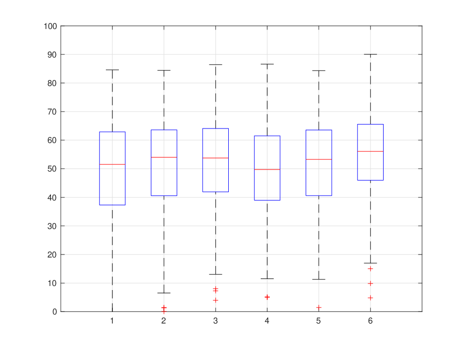
The simulation result is summarized below. The average model fits for the tested kernels are shown below:
| TC | DC | SSp | AMLS-2Os | AMLS-2Od | SI-2Od | |
| Avg. Fit | 47.5 | 50.0 | 50.9 | 48.4 | 49.7 | 53.3 |
The distribution of the model fits are shown in Fig. 6.
5.3.3 Findings
For the test systems and data bank, we have the following findings. The SI kernel (64) is best among all the tested kernels in both the average accuracy and robustness and thus is best to model systems with strong oscillation. The AMLS kernel (62b) works well as it is better than the TC kernel in both the average accuracy and robustness and it is just a bit worse than the DC kernel in the average accuracy. The AMLS kernel (62a) works not very well, though it has better average accuracy than the TC kernel. One possible explanation why the SI kernel (64) is best to model impulse response with strong oscillation is that the prior knowledge embedded in the SI kernel (64) is closest to the truth. This may be true because it makes use of the prior knowledge from a system theory perspective directly by choosing the nominal model to be a second order system with a pair of complex conjugate poles.
Remark 5.1
To embed the prior knowledge such as multiple distinct time constants and multiple resonant frequencies, we proposed to use the multiple kernel introduced in [7] where the multiple kernel is a conic combination of some fixed kernels. The fixed kernels can be instances of the SS, TC, DC and SI kernels (29) evaluated on a grid in their hyper-parameter space. The interested readers are referred to [7] for more details.
6 Conclusion
Kernel methods or regularization methods to estimate the impulse response of a linear time invariant systems is a most useful relatively recent addition to the techniques of system identification. Earlier results have demonstrated that important improvements in estimation quality can be achieved with kernels devised in a more or less ad hoc way. In this contribution, we have focused on systematic mechanisms and design concepts for how to construct kernels that are capable of adjusting its hyperparameters to capture the unknown system’s properties in useful ways. The two main avenues to such thinking have been a machine learning perspective focusing on function properties of the impulse response and a system theory perspective focusing on the LTI system that produces the impulse response. This has lead to understanding and insights into general properties of the earlier suggested methods, e.g. that the so called DC and SS kernels (derived from more ad hoc thinking) belong to the class of amplitude modulated locally stationary kernels (Proposition 3.2) and that they are simulation induced from certain LTI systems (Proposition 4.2). They are also related to maximum entropy optimal choices (Proposition 4.4) which is a valuable feature.
The take-home message of this contribution is as follows. The issue of kernel design should relate to the type of the prior knowledge and different types of prior knowledge should lead to different ways to design the corresponding kernels. Here, a machine learning perspective and a system theory perspective are introduced accordingly:
- •
Machine Learning perspective: If the impulse response is treated as a function and the prior knowledge is on its decay and varying rate, then we can design the amplitude modulated locally stationary (AMLS) kernel. In particular, we design a rank-1 kernel and a stationary kernel to account for the decay and varying rate of the impulse response, respectively. Moreover, by further exploiting the rank-1 kernel or the stationary kernel, it is possible to design AMLS kernels capable to embed more general prior knowledge.
- •
System Theory perspective: If the impulse is associated with an LTI system and the prior knowledge is that the LTI system is stable and may be overdamped, underdamped, have multiple distinct time constants and resonant frequencies and etc., then we can design the simulation induced (SI) kernel. In particular, the nominal model is used to embed the prior knowledge, the uncertainty is assumed to be stable and finally, the multiplicative uncertainty configuration is used to take into account both the nominal model and the uncertainty, and is simulated with an impulsive input to get the SI kernel or equivalently the zero-mean Gaussian process to model the impulse response.
Finally, finding a suitable kernel structure is only one leg of the kernel-based regularization method. Tuning its hyperparameters regardless of structure is the other main topic. This has been discussed in some detail e.g. in [4] and [8]. Some related new asymptotic results are recently presented in [9].
References
- [1] L. Ljung. System Identification - Theory for the User. Prentice-Hall, Upper Saddle River, N.J., 2nd edition, 1999.
- [2] T. Söderström and P. Stoica. System Identification. Prentice-Hall Int., London, 1989.
- [3] T. Chen, H. Ohlsson, and L. Ljung. On the estimation of transfer functions, regularizations and Gaussian processes - Revisited. Automatica, 48:1525–1535, 2012.
- [4] G. Pillonetto, F. Dinuzzo, T. Chen, G. De Nicolao, and L. Ljung. Kernel methods in system identification, machine learning and function estimation: A survey. Automatica, 50(3):657–682, 2014.
- [5] G. Pillonetto and G. De Nicolao. A new kernel-based approach for linear system identification. Automatica, 46(1):81–93, 2010.
- [6] G. Pillonetto, A. Chiuso, and G. De Nicolao. Prediction error identification of linear systems: a nonparametric Gaussian regression approach. Automatica, 47(2):291–305, 2011.
- [7] T. Chen, M. S. Andersen, L. Ljung, A. Chiuso, and G. Pillonetto. System identification via sparse multiple kernel-based regularization using sequential convex optimization techniques. IEEE Transactions on Automatic Control, (11):2933–2945, 2014.
- [8] Gianluigi Pillonetto and Alessandro Chiuso. Tuning complexity in regularized kernel-based regression and linear system identification: The robustness of the marginal likelihood estimator. Automatica, 51:106 – 117, 2015.
- [9] B. Mu, T. Chen, and L. Ljung. Tuning of hyperparameters for fir models – an asymptotic theory. In Proceedings of the IFAC 2017 World Congress, page under review, Toulouse, France., 2017.
- [10] A. N. Tikhonov and V. Y. Arsenin. Solutions of Ill-posed Problems. Winston/Wiley, Washington, D.C., 1977.
- [11] J Sjöberg, T McKelvey, and L Ljung. On the use of regularization in system identification. In Proceedings of the IFAC 2012 World Congress, pages 381–386, Sydney, Australia., 1993.
- [12] A. Chiuso. Regularization and Bayesian learning in dynamical systems: Past, present and future. Annual Reviews in Control, 41:24 – 38, 2016.
- [13] F. Dinuzzo. Kernels for linear time invariant system identification. SIAM Journal on Control and Optimization, 53(5):3299–3317, 2015.
- [14] Tianshi Chen and Lennart Ljung. Constructive state-space model induced kernels for regularized system identification. In 19th IFAC World Congress, pages 1047–1052, Cape town, South Africa, 2014.
- [15] T. Chen and L. Ljung. On kernel structure for regularized system identification (i): a machine learning perspective. In Proceedings of the IFAC Symposium on System Identification, pages 1035–1040, Beijing, China., 2015.
- [16] T. Chen and L. Ljung. On kernel structure for regularized system identification (ii): a system theory perspective. In Proceedings of the IFAC Symposium on System Identification, pages 1041–1046, Beijing, China., 2015.
- [17] Tianshi Chen, Tohid Ardeshiri, Francesca P. Carli, Alessandro Chiuso, Lennart Ljung, and Gianluigi Pillonetto. Maximum entropy properties of discrete-time first-order stable spline kernel. Automatica, 66:34 – 38, 2016.
- [18] F. P. Carli, T. Chen, and L. Ljung. Maximum entropy kernels for system identification. IEEE Transactions on Automatic Control, 2017.
- [19] A. Marconato, M. Schoukens, and J. Schoukens. Filter-based regularisation for impulse response modelling. IET Control Theory & Applications, to appear 2016.
- [20] K. Zhou, J. C. Doyle, and K. Glover. Robust and Optimal Control. Prentice-Hall, Englewood Cliffs, NJ, 1996.
- [21] T. Chen and L. Ljung. Implementation of algorithms for tuning parameters in regularized least squares problems in system identification. Automatica, 49:2213–2220, 2013.
- [22] Nachman Aronszajn. Theory of reproducing kernels. Transactions of the American mathematical society, pages 337–404, 1950.
- [23] Gianluigi Pillonetto and Alessandro Chiuso. Tuning complexity in regularized kernel-based regression and linear system identification: The robustness of the marginal likelihood estimator. Automatica, 58:106–117, 2015.
- [24] Claudio Carmeli, Ernesto De Vito, and Alessandro Toigo. Vector valued reproducing kernel hilbert spaces of integrable functions and mercer theorem. Analysis and Applications, 4(04):377–408, 2006.
- [25] Ingo Steinwart and Andreas Christmann. Support vector machines. Springer Science & Business Media, New York, 2008.
- [26] R Silverman. Locally stationary random processes. Information Theory, IRE Transactions on, 3(3):182–187, 1957.
- [27] C. E. Rasmussen and C. K. I. Williams. Gaussian Processes for Machine Learning. MIT Press, Cambridge, MA, 2006.
- [28] Akira Moiseevich Yaglom. Correlation theory of stationary and related random functions. Springer, 1987.
- [29] James Mercer. Functions of positive and negative type, and their connection with the theory of integral equations. Philosophical transactions of the royal society of London. Series A, containing papers of a mathematical or physical character, pages 415–446, 1909.
- [30] Harry Hochstadt. Integral equations. John Wiley & Sons, 1973.
- [31] Hongwei Sun. Mercer theorem for RKHS on noncompact sets. Journal of Complexity, 21(3):337–349, 2005.
- [32] Michel Loève. Probability theory, vol. II. Graduate texts in mathematics, 1978.
- [33] Brett Ninness and Graham C. Goodwin. Estimation of model quality. Automatica, 31(12):1771 – 1797, 1995.
- [34] L. Ljung. Model validation and model error modeling. In B. Wittenmark and A. Rantzer, editors, The �str�m Symposiium on Control, pages 15 –42, Lund, Sweden, Aug 1999. Studentlitteratur.
- [35] G. C. Goodwin, M. Gevers, and B. Ninness. Quantifying the error in estimated transfer functions with application to model order selection. IEEE Trans. Automatic Control, 37(7):913–929, 1992.
- [36] G. C. Goodwin, J. H. Braslavsky, and M. M. Seron. Non-stationary stochastic embedding for transfer function estimation. Automatica, 38:47–62, 2002.
- [37] Wolfgang Reinelt, Andrea Garulli, and Lennart Ljung. Comparing different approaches to model error modeling in robust identification. Automatica, 38(5):787 – 803, 2002.
- [38] Model Error Modeling and Stochastic Embedding, volume 48, Beijing, China, 2015.
- [39] C. Chen. Linear system theory and design. Oxford University Press, New York, 3 edition, 1999.
- [40] Torkel Glad and Lennart Ljung. Control theory: Multivariable and nonlinear methods. Taylor & Francis, 2000.
- [41] T. B. Schön, A. Wills, and B. Ninness. System identification of nonlinear state-space models. Automatica, 47(1):39–49, January 2011.
- [42] K. J. Åström. Introduction to stochastic control theory. Academic Press, New York and London, 1970.
- [43] E. T Jaynes. On the rationale of maximum-entropy methods. Proceedings of the IEEE, 70(9):939–952, 1982.
- [44] F. P. Carli. On the maximum entropy property of the first-order stable spline kernel and its implications. In IEEE Multi-Conference on Systems and Control, pages 409–414, Nice/Antibes, France, 2014.
- [45] A. Chiuso, T. Chen, L. Ljung, and G. Pillonetto. On the design of multiple kernels for nonparametric linear system identification. In Proceedings of the IEEE Conference on Decision and Control, pages 3346–3351, Los Angeles, CA., 2014.
- [46] Marc G Genton. Classes of kernels for machine learning: a statistics perspective. The Journal of Machine Learning Research, 2:299–312, 2002.
- [47] Theodoros Evgeniou, Massimiliano Pontil, and Tomaso Poggio. Regularization networks and support vector machines. Advances in computational mathematics, 13(1):1–50, 2000.
- [48] F. Cucker and S. Smale. On the mathematical foundations of learning. American Mathematical Society, 39(1):1–49, 2002.
- [49] T. M. Cover and J. A. Thomas. Elements of information theory. John Wiley & Sons, 2012.
- [50] A. P. Dempster. Covariance selection. Biometrics, 28(1):157–175, 1972.
Proof of Proposition 3.1
Part (a). For any and for any , , let be the column vector containing in order. Then the kernel matrix defined by is rewritten as . Clearly, is positive semidefinite, and moreover . So is a rank-1 kernel by definition. The identity (19), Part (b) and Part (c) can be verified in a straightforward way.
Proof of Proposition 3.2
We give the proof for the CT case with . The results for the DT case with hold by noting that the DT kernel is the CT kernel restricted to .
From (21) and (22), we see the proof will be done if it can be shown that the kernels in (21) and (22) are stationary kernels. To show this, note from e.g. [27, page 85] that with is called the exponential kernel and belongs to the class of Matérn covariance functions with order . So it remains to show in (21) is also a kernel. Note that the exponential kernel is an isotropic stationary (IS) kernel (see Section 3.2.1 for its definition). Below we show that in (21) is actually also an IS kernel. As shown in [46], the spectral representation of an IS kernel takes the form of
| (66) |
where is any nondecreasing bounded function. For the exponential kernel with , (66) is satisfied with the spectral density
So in (21) with satisfies (66) with a well defined spectral density described by
Therefore, in (21) is an IS kernel. This completes the proof.
Proof of Proposition 3.3
We give the proof for the CT case with . The proof for the DT case with can be derived in a similar way.
Part (a). Assume that , i.e., . Since for any . Then from
Part (b). Assume that the AMLS kernel (18) is stable, i.e., . We need a lemma to prove the result.
Lemma A.1
[47, p. 16], [48, p. 37] Assume that with is a positive semidefinite kernel and moreover, there exists a sequence of positive numbers and linearly independent functions such that , where the convergence is absolute and uniform on with being any compact subsets of . Then
and for any with and , the inner product over is defined as
Noting (24) and by Lemma A.1, we have
| (67) |
Then from (24), the AMLS kernel (18) is rewritten as
| (68) |
and by Lemma A.1, we have
| (69) |
| (70) |
Since , for any , , i.e.,
| (71) |
where the equality follows from (70) and is the function associated with .
Since is not stable, and there exists but . For such , if there exits an such that for all , then
which contradicts with (71). This completes the proof.
Proof of Proposition 4.1
To prove the result, we need a lemma.
Lemma A.2
[42, 40] Consider a zero mean stationary Gaussian process with covariance function . Assume that has rational power spectral density 88 8 Check the statement of Theorem 4.1 for the definition of rational power spectral density. . Then the following results hold:
- •
For the DT case, there exists a rational function which has all poles inside the unit circle and all zeros inside or on the unit circle such that
(72) where denotes the modulus of a complex number. Moreover, let the quintuple be a state space realization of , i.e., , where is the dimension of and is the identity matrix with dimension . Then the stationary Gaussian process has the following state space representation
(73a) (73b) where is the zero mean white Gaussian noise with unit variance and is the solution of the Lyapunov equation (73c) - •
For the CT case, there exists a rational function which has all poles in the left half plane and all zeros in the left half plane or on the imaginary axis such that
(74) Moreover, let the quintuple be a state space realization of , i.e., . Then the stationary Gaussian process has the following state space representation
(75a) (75b) where is the zero mean white Gaussian noise with unit power spectral density and is the solution of the Lyapunov equation (75c)
Proof: For the DT case, the first part is a result of the Spectral Factorization Theorem [42, Theorem 3.1 in Chapter 4] and the second part is a result of the Representation Theorem [42, Theorem 3.2 in Chapter 4] and [40, Theorem 5.3 and Equation (5.92)]. For the CT case, the first part is a result of the Spectral Factorization Theorem [42, Theorem 5.1 in Chapter 4] and the second part is a result of the Representation Theorem [42, Theorem 5.2 in Chapter 4] and [40, Theorem 5.3]. .
Proof of Proposition 4.2
We only sketch the proof for the SS kernel and the proof for the DC kernel can be derived in a similar way.
For the DT case, the IS kernel in (21) has the power spectral density
By spectral factorization technique, we have with
For the CT case, the IS kernel has the power spectral density
From the realization theory of linear systems, see e.g., [39], we can derive the corresponding state-space model representation of the IS kernel , based on which and by using the argument in the end of the proof of Proposition 4.1, we derive (• ‣ 4.2) and (• ‣ 4.2), respectively.
Proof of Proposition 4.3
Proof of Proposition 4.4
We only give the proof for the case and the proof for the case (b) is similar and thus omitted.
By chain rule, the differential entropy in (52) becomes
| (76) |
Note from (51) that
where the first equation follows because translation does not change the differential entropy and the second equation follows because of the scaling property of differential entropy. Analogously, we have
Therefore, (76) is rewritten as
Since the second term in the above equation is independent of and , , the MaxEnt problem (52) is equivalently rewritten as
| (77a) | ||||
| subject to | ||||
| (77b) | ||||
Note that the constraints in (77) are separable with respect to , , and that is maximized if , are independent with each other. Therefore, (77) is equivalent to
and for ,
It is well known that multivariate normal distribution maximizes the differential entropy over all distributions with the same covariance, see e.g., [49, Theorem 8.6.5]. Then we have the optimal solution to (77) is that and , , and moreover, are independent with each other. Finally, (51) implies , same as in (30a). This completes the proof.
Proof of Corollary 4.1
From Proposition 4.2, the DC kernel is a SI kernel with given in (41), which implies that Theorem 4.4 holds for the DC kernel. Comparing (51) with (55) shows that the proof is completed if we can show
| (78) |
The first line of (78) is straightforward. In what follows, we consider the second line of (78). Clearly, the results holds for the case either or . So we further consider below the case where and . It is easy to see that for ,
where the second equality holds because . Therefore (78) holds, which completes the proof.
Proof of Proposition 4.5
We need a lemma to prove this result.
Lemma A.3
Consider the th order Gaussian Markov process (57). Then the following results hold:
- (a)
For any and , and are conditionally independent given with , and .
- (b)
Let with be any strictly increasing subsequence taken from . Then the covariance matrix of is a -band matrix.
Proof: Part (a) follows from the th order Markov property of and the fact that is white Gaussian noise. To prove Part (b), recall from e.g., [50] that, for Gaussian random variables, the zeros in the inverse of the covariance matrix indicate conditional independence of the two corresponding elements conditioned on the remaining ones. To be specific, consider a Gaussian random variable with mean and covariance matrix :
where , and . Then for a given , are conditionally independent if and only if , where denote the th element of . Therefore, Part (b) follows from the above observation and part (a).
Proof of Proposition 4.6
By using the realization of in controllable canonical form, the DT SI kernel (29) is written as follows: