The spinon Fermi surface U(1) spin liquid in a spin-orbit-coupled
triangular lattice Mott insulator YbMgGaO4
Abstract
Motivated by the recent progress on the spin-orbit-coupled triangular lattice spin liquid candidate YbMgGaO4, we carry out a systematic projective symmetry group analysis and mean-field study of candidate U(1) spin liquid ground states. Due to the spin-orbital entanglement of the Yb moments, the space group symmetry operation transforms both the position and the orientation of the local moments, and hence brings different features for the projective realization of the lattice symmetries from the cases with spin-only moments. Among the eight U(1) spin liquids that we find with the fermionic parton construction, only one spin liquid state, that was proposed and analyzed in Yao Shen, et. al., Nature 540, 559-562 (2016) and labeled as U1A00 in the present work, stands out and gives a large spinon Fermi surface and provides a consistent explanation for the spectroscopic results in YbMgGaO4. Further connection of this spinon Fermi surface U(1) spin liquid with YbMgGaO4 and the future directions are discussed. Finally, our results may apply to other spin-orbit-coupled triangular lattice spin liquid candidates, and more broadly, our general approach can be well extended to spin-orbit-coupled spin liquid candidate materials.
I Introduction
The interplay between strong spin-orbit coupling (SOC) and strong electron correlation has attracted a significant attention in recent years [1]. At the mean time, the abundance of strongly correlated materials with and electrons, such as iridates and rare-earth materials [1, 2], brings a fertile arena to explore various emergent and exotic phases that arise from such an interplay [3, 4, 5, 6, 7, 8, 9, 10, 11, 12, 13, 14, 15, 16, 17, 18, 19, 20, 21, 22, 23, 24, 25, 26, 27, 28, 29, 30, 31, 32]. The recently discovered quantum spin liquid (QSL) candidate YbMgGaO4 [33], where the rare-earth Yb atoms form a perfect triangular lattice, is an ideal system that involves strong spin-orbital entanglement in the strong Mott insulating regime of the Yb electrons [34, 35, 36, 37, 38, 39, 40, 41].
In YbMgGaO4, the thirteen electrons of the Yb3+ ions are well localized and form a spin-orbit-entangled total moment with [34, 35]. The eight-fold degeneracy of the moment is further split by the crystal electric fields. The resulting ground state Kramers doublet of the Yb3+ ion, whose two-fold degeneracy is protected by the time-reversal symmetry, is well separated from the excited doublets and is responsible for the low-temperature magnetic properties of YbMgGaO4. No signature of time-reversal symmetry breaking is observed for YbMgGaO4 down to the lowest measured temperature [38, 37, 36]. Applying the recent theoretical result on spin-orbit-coupled Mott insulators [42], two of us and collaborators have proposed YbMgGaO4 to be the first QSL candidate in the spin-orbit-coupled Mott insulator with odd electron fillings [34, 35, 36, 39]. More broadly, YbMgGaO4 represents a new class of rare-earth materials where the strong spin-orbit entanglement of the local moments meets with the geometrical frustration of the triangular lattice such that exotic quantum phases may be stabilized.

Apart from the absence of magnetic ordering, the heat capacity was found to be at low temperatures [33, 34, 37, 43], and is close to the well-known heat capacity [44, 45, 46]. The latter was the one obtained within a random phase approximation for the spinon-gauge coupling in a spinon Fermi surface U(1) QSL [44, 45, 46]. More substantially, the broad continuum [36, 37] of the magnetic excitation with a clear dispersion for the upper excitation edge agrees reasonably with the particle-hole continuum of the spinon Fermi surface [36]. However, due to the scattering with the phonon degrees of freedom, the thermal transport measurement in YbMgGaO4 was unable to extract the intrinsic magnetic contribution to the thermal conductivity [43]. Partly motivated by the spin liquid behaviors in YbMgGaO4 and more broadly by the families of rare-earth magnets with identical structures, in this paper, we carry out a systematic projective symmetry group (PSG) analysis for a triangular lattice Mott insulator with spin-orbital-entangled local moments. Unlike the cases for the spin-only moments in the pioneering work by X.-G. Wen [47], the space group symmetry operation, in particular, the rotation, transforms both the position and the orientation of the Yb local moments [35, 39]. We find that, among the eight U(1) QSL states, the spinon mean-field state that was introduced in Ref. 36 and labeled as the U1A00 state in our PSG classification, contains a large spinon Fermi surface and gives a large spinon scattering density of states that is consistent with the inelastic neutron scattering (INS) results.
The following part of the paper is organized as follows. In Sec. II, we describe the space group symmetry and the the multiplication rules for the symmetry transformation. In Sec. III, we introduce the fermionic spinon construction and the fermionic spinon mean-field Hamiltonian. In Sec. IV, we explain the scheme for the projective symmetry group classification when the spin-orbit coupling is present. In Sec. V, we explain the relationship between the spinon band structure and the projective symmetry group of the spinon mean-field states. In Sec. VI, we focus on the U1A00 state and study the spectroscopic properties of this state. Finally in Sec. VII, we discuss the experimental relevance and remark on the thermal transport result and the competing scenarios and proposals. The details of the calculation are presented in the Appendices.
II Space group symmetry
It was pointed out that the intralayer symmetries involves two translations, and , one two-fold rotation, , one three-fold rotation, , and one spatial inversion (see Fig. 1(a)) [35, 39]. Here we use a different complete set of elementary transformations for the space group symmetries that involve two translations, and , one two-fold rotation, , and one more operation, (see the definition in Fig. 1(b)). It is ready to confirm with the definition . The multiplication rules of this symmetry group is given as
| (1) | |||||
| (2) | |||||
| (3) | |||||
| (4) |
Due to the presence of time reversal in YbMgGaO4 [34, 38, 36, 37], we further supplement the symmetry group with the time reversal such that and , where is a lattice symmetry operation.
| U(1) QSL | ||||
|---|---|---|---|---|
| U1A00 | ||||
| U1A10 | ||||
| U1A01 | ||||
| U1A11 |
III Fermionic parton construction
To describe the U(1) QSL that we propose for YbMgGaO4, we introduce the fermionic spinon operator ) that carries spin-1/2, and express the Yb local moment as
| (5) |
where is a vector of Pauli matrices. We further impose a constraint on each site to project back to the physical Hilbert space of the spins. The choice of fermionic spinons allows a local SU(2) gauge freedom [47].
As a direct consequence of the spin-orbital entanglement, the spinon mean-field Hamiltonian for the U(1) QSL should generically involve both spin-preserving and spin-flipping hoppings, and has the following form
| (6) |
where is the spin-dependent hopping. The choice of the mean-field ansatz in Eq. (6) breaks the local SU(2) gauge freedom down to U(1). Here, to get a more compact form for Eq. (6), we follow Ref. 49 and introduce the extended Nambu spinor representation for the spinons such that and
| (7) |
where is a hopping matrix that is related to . With the extended Nambu spinor, the spin operator and the generator for the SU(2) gauge transformation are given by [47, 50, 51, 52, 53]
| (8) | |||||
| (9) |
where is a identity matrix. Under the symmetry operation , transforms as
| (10) |
where is the local gauge transformation that corresponds to the symmetry operation , and we add a spin rotation because the spin components are transformed when involves a rotation. In Eq. (10), the gauge transformation and the spin rotation are commutative [54] simply because . Moreover, from Eq. (9), the gauge transformation is block diagonal with , where is a matrix (see Appendix).
IV Projective symmetry group classification
For the spinon mean-field Hamiltonian in Eq. (6), the lattice symmetries are realized projectively and form the projective symmetry group (PSG). To respect the lattice symmetry transformation , the mean-field ansatz should satisfy
| (11) |
The ansatz itself is invariant under the so-called invariant gauge group (IGG) with . The IGG can be regarded as a set of gauge transformations that correspond to the identity transformation. For an U(1) QSL, IGG = U(1).
A general group relation for the lattice symmetry turns into the following group relation for the PSG
| (12) | |||||
| (13) |
where we used the fact that the gauge transformation commutes with the spin rotation. As the series of rotations either rotate the spinons by or ,
| (14) |
where is a identity matrix. Since , then
| (15) |
This immediately indicates that, to classify the PSGs for a spin-orbit-coupled Mott insulator, we only need to focus on the gauge part, first find the gauge transformation with the same procedures as those for the conventional Mott insulators with spin-only moments [47], and then account for the spin rotation.
For the mean-field ansatz in , we choose the “canonical gauge” for the IGG with
| (16) |
Under the canonical gauge, the gauge transformation associated with the symmetry operation takes the form of
| (17) | |||||
where . For translations, one can always choose a gauge such that
| (18) | |||||
| (19) |
with and . The group relation in Eq. (3) further demands . Thus the group relation in Eq. (1) gives , where is the flux through each unit cell of the triangular lattice and takes the value of (see Appendix). The PSGs with are labeled by U1A (U1B). Among the sixteen algebraic PSGs that we find, eight unphysical solutions have for the spinons and give vanishing spinon hoppings everywhere. In Tab. 1 and the Appendix, we list the remaining eight PSGs that have consistent with the fact that fermionic spinons are Kramers doublets (see Appendix).


V Mean-field states
Here we obtain the spinon mean-field Hamiltonian from Tab. 1 and explain why the U1A00 state stands out as the candidate ground state for YbMgGaO4. We start with the U1A states. Among the four U1A states, the U1A10 state gives a vanishing mean-field Hamiltonian for the spinon hoppings between the first and the second neighbors, the remaining ones except the U1A00 state all have symmetry protected band touchings at the spinon Fermi level (see Fig. 2). To illustrate the idea [55], we consider the U1A01 state where the spinon Hamiltonian has the form in the momentum space and is a matrix with
| (20) |
For this band structure there are nondegenerate band touchings at , M and K points that are protected by the PSG of the U1A01 state. Under the operation , the PSG demands that spinons to transform as
| (21) | |||||
| (22) |
Applying three times and keeping invariant, we require
| (23) |
which forces . The time reversal symmetry () further requires that . Thus we have symmetry protected band touchings with at the time reversal invariant momenta and M. The K points are invariant under and because the spinon partile-hole transformation is involved for (see Appendix). Using those two symmetries, we further establish the band touching at the K points. Likewise, for the U1A11 state, the PSG demands the band touchings at and M points. Because there are only two spinon bands for the U1A states, these band touchings generically occur at the spinon Fermi level.
Due to the Dirac band touchings at the Fermi level, the low-energy dynamic spin structure factor, that measures the spinon particle-hole continuum, is concentrated at a few discrete momenta that correspond to the intra-Dirac-cone and the inter-Dirac-cone scatterings [36]. Clearly, this is inconsistent with the recent INS result that observes a broad continuum covering a rather large portion of the Brillouin zone [36, 37].
For the U1B states, the spinons experience a background flux in each unit cell. The direct consequence of the background flux is that the U1B states support an enhanced periodicty of the dynamic spin structure in the Brillouin zone [56, 47, 57]. Such an enhanced periodicity is absent in the INS result [36, 37]. In particular, unlike what one would expect for an enhanced periodicity, the spectral intensity at the point is drastically different from the one at the M point in the existing experiments [36, 37].
The above analysis leads to the conclusion that the U1A00 state is the most promising candidate U(1) QSL for YbMgGaO4, and this conclusion is independent from any microscopic model. The spinon mean field Hamiltonian, allowed by the U1A00 PSG, is remarkably simple and is given as 11 1 In the previous work [36], only the nearest-neighbor spinon hopping is included.
| (24) |
where the spinon hopping is isotropic for the first and the second neighbors. This mean-field state only has a single band that is 1/2-filled, so it has a large spinon Fermi surface. From , we construct the mean-field ground state by filling the spinon Fermi sea,
| (25) |
where is the spinon dispersion and is the spinon Fermi energy. The mean-field variational energy is
| (26) |
where
| (27) | |||||
is the microscopic spin model that was introduced in Refs. 34, 35, and is a bond-dependent phase factor due to the spin-orbit-entangled nature of the Yb moments [35]. The anisotropic nature of the spin interaction has been clearly supported by the recent polarized neutron scattering measurement [59]. For the specific choice with , we find the minimum variational energy and occurs at (see Appendix). Here, the expectation values of the and interactions simply vanish, and this is an artifact of the free spinon mean-field theory with the isotropic hoppings in Eq. (24). We here establish that the U1A00 state is a spinon Fermi surface U(1) QSL.
VI Spectroscopic properties
For the U1A00 state, the dynamic spin structure essentially detects the spinon particle-hole excitation across the Fermi surface. The information about the Fermi surface is encoded in the profile of the dynamic spin structure factor. We evaluate the dynamic spin structure factor within the free spinon mean-field theory (see Appendix) (see Fig. 3(a)). Qualitatively similar to the mean-field theory with only first neighbor spinon hoppings, the improved free-spinon mean-field theory of captures the crucial features of the INS results [36, 37]. The spinon particle-hole continuum covers a large portion of the Brillouin zone, and vanishes beyond the spinon bandwidth. More importantly, the “V-shape” upper excitation edge near the point in Fig. 3(a) was clearly observed in the experiments [36, 37], and the slope of the “V-shape” is the Fermi velocity.


Due to the isotropic spinon hoppings, does not explicitly reflect the absence of spin-rotational symmetry that is brought by the and interactions. To incorporate the and interactions, we follow the phenomenological RPA treatment for the “-” model in the context of cuprate superconductors [60] and consider
| (28) |
where are the and interactions (see Appendix). While the free spinon results from already capture the main features of the neutron scattering data [36, 37], the anisotropic spin interaction , included by RPA, merely redistributes the spectral weight in the momentum space. We find in Fig. 3(b) that, the low-energy spectral weight at M is slightly enhanced, a feature observed in Refs. 36, 37. From our choice of the parameters, it is plausible that this peak results from the proximity to a phase with a stripe-like magnetic order [36, 35, 39].
VII Discussion
We have demonstrated that the spinon Fermi surface U(1) QSL gives a consistent explanation of the INS result in YbMgGaO4. Moreover, the anisotropic spin interaction, slightly enhances the spectral weight at the M points. The U(1) gauge fluctuation in the spinon Fermi surface U(1) QSL [45, 44] was suggested to be the cause for the sublinear temperature dependence of the heat capacity in YbMgGaO4 [36, 46, 35, 39].
In YbMgGaO4, the coupling between the Yb moments is relatively weak [34]. It is feasible to fully polarize the spin with experimentally accessible magnetic fields [35, 37, 39, 61] and to study the evolution of the magnetic properties under the magnetic field. Recently, two of us have predicted the spectral weight shift of the INS for YbMgGaO4 under a weak magnetic field [41], and the predicted spectral crossing at the point and the dispersion of the spinon continuum have actually been confirmed in the recent INS measurement [62]. Numerically, it is useful to perform numerical calculation with fixed and that are close to the ones for YbMgGaO4, and obtain the phase diagram of our spin model by varying and [35, 39, 63]. More care needs to be paid to the disordered region of the mean-field phase diagram [35] where quantum fluctuation is found to be strong [35]. The “” oscillation in the spin correlation would be the strong indication of the spinon Fermi surface. Noteworthily recent DMRG works [64, 65] have actually provided some useful information about the ground states of the system, in particular, Ref. 65 suggested the scenario of exchange disorders. Certain amount of exchange disorder may be created by the crystal electric field disorder that stems from the Mg/Ga mixing in the non-magnetic layers [61, 37], but recent polarized neutron scattering measurement did not find strong exchange disorder [59]. Regardless of the possibilities of exchange disorders, the spin quantum number fractionalization, that is one of the key properties of the QSLs, could survive even with weak disorders. The approach and results in our present work are phenomenologically based and are independent of the microscopic mechanism for the possible QSL ground state in YbMgGaO4.
Ref. 43 claimed the absence of the magnetic thermal conductivity in YbMgGaO4 by extrapolating the low-temperature thermal conductitivity data in the zero magnetic field. Here, we provide an alternative understanding for this thermal transport result. The hint lies in the field dependence of the thermal conductivity. It was found that, when strong magnetic fields are applied to YbMgGaO4, the thermal conductivity at 0.2K is increased compared with the one at zero field [43]. If one ignores the disorder effect and assumes the zero-field thermal conductivity is a simple addition of the magnetic contribution and the phonon contribution with
| (29) |
the strong magnetic field almost polarizes the spins completely and creates a spin gap for the magnon excitation, hence suppress the magnetic contribution. The high-field thermal conductivity would be purely given by the phonon contribution, and we would expect a decreasing of the thermal conductivity in the strong field compared to the zero field result. This is clearly inconsistent with the experimental result. Therefore, the zero-field thermal conductivity is not a simple addition of the magnetic contribution and the phonon contribution, i.e.,
| (30) |
This also strongly suggests the presence rather than the absence of magnetic excitations in the thermal conductivity result at zero magnetic field. If there is no magnetic excitation in the system at low temperatures, the low-temperature thermal conductivity at zero field should just be the phonon contribution, and we would expect the zero-field thermal conductivity to be the same as the one in the strong field limit, (although the intermediate field regime could be different). This is again inconsistent with the experiments. This means that the magnetic excitation certainly does not have a large gap and could just be gapless as we propose from the spinon Fermi surface state. In fact, the gapless nature of the magnetic excitation is consistent with the power-law heat capacity results in YbMgGaO4. What suppresses could arise from the mutual scattering between the magnetic excitations and the the phonons. In fact, similar field dependence of thermal conductivity has been observed in other rare-earth systems such as Tb2Ti2O7 [66, 67, 68] and Pr2Zr2O7 [69]. It was suggested there [67, 68, 69] that the spin-phonon scattering is the cause. The Yb local moment, that is a spin-orbit-entangled object, involves the orbital degree of freedom. The orbital degree of freedom is sensitive to the ion position, and thus couples to the phonon strongly. This is probably the microscopic origin for the strong coupling between the magnetic moments and the phonons in the rare-earth magnets. This is quite different from the organic spin liquid candidates and the herbertsmithite kagome system where the orbital degree of freedom does not seem to be involved [70, 71, 72, 73].
If the ground state of YbMgGaO4 is a QSL with the spinon Fermi surface, the field-driven transition from the QSL ground state to the fully polarized state is necessarily a unconventional transition beyond the traditional Landau’s paradigm and has not been studied in the previous spin liquid candidates [70, 71, 72, 73]. The smooth growth of the magnetization with varying external fields indicates a continuous transition [34]. Since we propose YbMgGaO4 to be a spinon Fermi surface U(1) QSL and gapless, the transition would be associated with the openning of the spin gap at the critical field. The continuous nature of the transition suggests the spin gap to open in a continuous manner. Moreover, the spinon confinement would be concomitant with the spin gap that suppresses the spinon density of states and allows the instanton events of the U(1) gauge field to proliferate. Therefore, it might be interest to identify the critical field and obtain the critical properties of the field-driven transition. Thermodynamic, spectroscopic, and thermal transport measurements with finer field variation would be helpful.
Finally, several families of rare-earth triangular lattice magnets have been discovered recently [35, 39, 74, 75, 76, 77, 78, 79]. Their properties have not been studied carefully. Our general classification results and the prediction of the spectroscopic properties would apply to the QSL candidates that may emerge in these families of materials. It is certainly exciting if one finds the new QSL candidates in these families behave like YbMgGaO4 [35].
VIII Acknowledgements
We thank one anonymous referee for the suggestion for improvement to this paper, and Zhu-Xi Luo for pointing out some typos. G.C. acknowledges the discussion with Xuefeng Sun from USTC and Yuji Matsuda about thermal transports in rare-earth magnets, and the discussion with Professor Sasha Chernyshev about the related matters. This work is supported by the Ministry of Science and Technology of China with the Grant No.2016YFA0301001 (G.C.), the Start-Up Funds of OSU (Y.M.L.) and Fudan University (G.C.), the National Science Foundation under Grant No. NSF PHY-1125915 (Y.M.L and G.C.), the Thousand-Youth-Talent Program (G.C.) of China, and the first-class university construction program of Fudan University.
Appendix A The coordinate System and space group symmetry
Following our convention in Fig. 1 in the main text, we choose the coordinate system of the triangular lattice to be
| (31) | |||||
| (32) |
We label the triangular lattice sites by . Restricted to the triangular layer, the space group contains two translations along the direction, along the direction, a counterclockwise three-fold rotation around the lattice site, a two-fold rotation around , and the inversion at the lattice site. Their actions on the lattice indices are
| (33) | |||||
| (34) | |||||
| (35) | |||||
| (36) | |||||
| (37) |
In the formulation introduced in the main text, we consider an equivalent set of generators, , where the operation is defined as and acts on the lattice indices as
| (38) |
It is evident that these two sets of generators are equivalent, since we merely redefine the symmetry rather than introducing any new symmetry.
The multiplication rule of this symmetry group is given in the main text. For the convenience of the presentation below, we also list these rules here,
| (39) | |||||
| (40) | |||||
| (41) | |||||
| (42) |
Including the time reversal symmetry, we further have
| (43) | |||||
| (44) | |||||
| (45) |
Appendix B Projective symmetry group classification
As we describe in the main text, we consider the U(1) QSL. The spinon mean-field Hamiltonian has the following form
| (46) |
where is the spin-dependent hopping. With the extended Nambu spinor representation [49] , has a more compact form
| (47) |
where is a hopping matrix that is related to ,
| U(1) QSL | ||||
|---|---|---|---|---|
| U1A00 | ||||
| U1A10 | ||||
| U1A01 | ||||
| U1A11 | ||||
| U1B00 | ||||
| U1B10 | ||||
| U1B01 | ||||
| U1B11 |
B.1 Spatial symmetry
First of all, the gauge transformation and spin rotation are commutative. So in the PSG classification, we only need to focus on the gauge part of the PSG transformation. In the canonical gauge , the gauge transformation associated with a given symmetry operation takes the form
| (53) |
where . For the symmetry multiplication rule where is an unitary transformation, the corresponding PSG relation becomes
| (54) |
or equivalently,
| (55) |
We start with and , where
| (56) | |||||
| (57) |
Through Eq. (40) that connects and , one immediately has . From Eq. (41) where the total number of and is odd, one immediately has . So we have
| (58) | |||||
| (59) |
Using Eq. (39), we have
| (60) |
which leads to the result
| (61) |
with to be determined. Since it is always possible to choose a gauge such that , then we have .
Similarly, leads to
| (62) |
It is ready to find .
We continue to find and . For the operation with , Eq. (41) leads to
| (63) | |||||
| (64) |
for , and
| (65) | |||||
| (66) |
for . So we obtain
| (67) | |||
| (68) |
For , we further require . is automatically satisfied with the above relations for both and .
For with , we need to consider two separate cases with , respectively. If , Eq. (40) leads to
| (69) | |||||
| (70) |
So we obtain and for . Similary, for , we obtain .
Using , we further have for , and for . So we arrive at the result
| (71) | |||||
| (72) |
Here, to simplify the above expression, we choose a pure gauge tranformation . Under the pure gauge transformation, the gauge part of the PSG transforms as
| (73) |
Clearly only modifies and by an overall phase shift, but becomes
| (74) |
for both , except that we require for .
For the relation , we need to consider the four cases with and .
For , we have , and gives . We then introduce a pure gauge transformation ,
| (75) |
After applying , we have
| (76) | |||||
| (77) |
with .
For and , we obtain . We introduce a pure gauge transformation ,
| (78) |
After applying , we have
| (79) | |||||
| (80) |
For and , we obtain . We apply a pure gauge transformation and obtain
| (81) | |||||
| (82) |
For and , we obtain . We apply a pure gauge transformation and obtain
| (83) | |||||
| (84) |
In summary, we have
| (85) |
and
| (86) | |||||
| (87) |
where for or .
B.2 Time reversal symmetry
Because time reversal is an antiunitary symmetry, the product becomes
| (88) |
for the PSGs, where is the gauge transformation associated with the time reversal. We here redefine
| (89) |
so that
| (90) |
has the general form .
We start with . The relation in Eq. (43) leads to
| (91) | |||||
| (92) |
so we have . Applying this result to Eq. (44), we have
| (93) |
for . The above equations give , so we have . Other cases can be obtained likewise. We find that for both and , there is and . So we have
| (94) |
where we have used a global and uniform rotation to rotate to the basis of .
Including the time reversal, there are 16 PSG solutions. But for , the mean-field ansatz is found to vanish everythere. This makes sense as these PSGs have for the fermionic spinons that are expected to Kramers doublets. So only 8 of them with for the spinons survive. Replacing with , we present the PSG solutions in the table of the main text.
Appendix C Spinon band structures and mean-field Hamiltonians
As we establish in the previous section and the main text, there are four U1A PSGs and four U1B PSGs. In the main text, we have argued that the experimental resuls in YbMgGaO4 is against the U1B states. So here we focus on the U1A states. From the U1A PSGs, it is straight to obtain the spinon transformations. We list the results in Tab. 3.
| U(1) PSGs | ||||
|---|---|---|---|---|
| U1A00 | ||||
| U1A10 | ||||
| U1A01 | ||||
| U1A11 |
C.1 Spinon band structures
Using Tab. 3, we obtain the spinon mean-field Hamiltonian. In particular, the U1A10 state gives vanishing spinon hoppings on the first and second neighbors, and the U1A01 state gives an isotropic spinon hopping on both first and second neighbors. The U1A10 state, as we described in the main text, has symmetry protected band touchings at the , M and K points. The U1A11 state has symmetry protected band touchings at the and M points.
For the U1A10 state, the spinon mean-field Hamiltonian has the form
| (95) |
where is given by
| (96) |
In the main text, we have used and to show and the band touchings at and M. To account for the band touching at the K point, we need to use and . Under ,
| (97) | |||||
where . Since K is invariant under ,
| (98) |
hence .
The symmetry constraints the term, we have
| (99) | |||||
Since K is also invariant under , we obtain . Hence . We conclude that and there exists a band touching at K.
For the U1A11 state, and are implemented in the same way as the U1A01 state, and we arrive at the same conclusion that there are band touchings at the and M points. At the K point, however, the band structure is generally gapped due to a nonzero .
C.2 Spinon mean-field Hamiltonians
The U1A00 state has the isotropic spinon hoppings on first and second neighboring bonds, and the mean-field Hamiltonain has already been given in the main text. This states gives a large spinon Fermi surface in the Brioullin zone. The spinon mean-field states of the U1A01 state and the U1A11 state are given by
| (100) | |||||
and
| (101) | |||||
where in both Hamiltonians , denote the first neighbor hoppings and denotes the second neighbor hopping.
The band structures for specific choices of the hopping parameters are plotted in the main text. Clearly, we observe the band touchings at the , M and K points for the U1A01 state, and band touchings at the and M points for the U1A11 state.
Appendix D The U1A00 state and the spectroscopic results
D.1 Free spinon mean-field theory
The spinon mean-field Hamiltonian of the U1A00 state is
| (102) |
from which we compute the dynamic spin structure factor for different choices . The dynamic spin structure factor is given by
| (103) | |||||
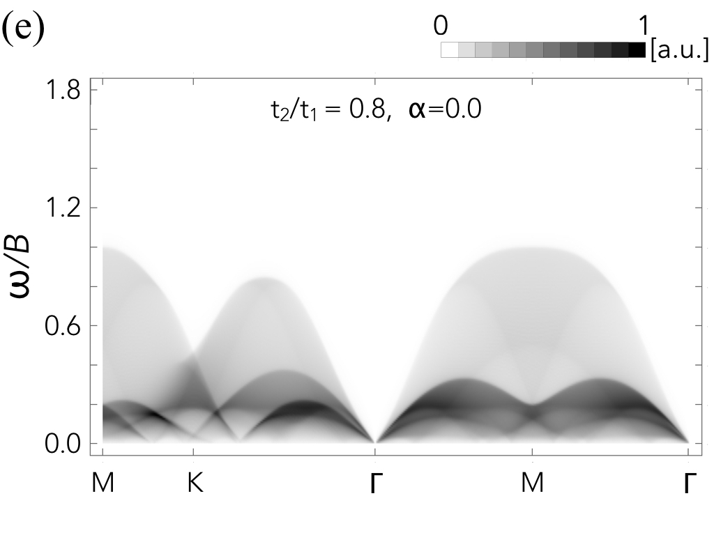
where is the total number of spins, the summation is over all mean-field states with the spinon particle-hole excitation, is the energy of the -th excited state with the momentum . The results are depicted in Fig. 4(a-e) and are consistent with the inelastic neutron scattering results [36, 37]. All the results so far are independent from any microscopic spin interaction.




D.2 Variational calculation and random phase approximation
Here we consider the microscopic spin Hamiltonian that was introduced in Refs. 34, 35,
| (104) | |||||
where for along the and bonds, respectively. Here, . It was suggested and demonstrated that the anisotropic and interactions compete with the XXZ part of the Hamiltonian and may lead to disordered state [34, 35, 39]. Our calculation does show the enhancement of quantum fluctuation in certain regions of the phase diagram [35]. Here we comment about the choices of the exchange couplings in the main text and in the following calculation. The and couplings can be determined by the Curie-Weiss temperature measurement on a single crystal sample. The complication comes from the subtraction of the Van Vleck susceptibility. Due to the Ga3+/Mg2+ exchange disorder in the non-magnetic layers, although these ions do not directly enter the Yb exchange path, it may modify the local crystal field environment of the Yb3+ ion and thus lead to some complication and variation of the Van Vleck susceptibility. As a result, the very precise determination of the and couplings can be an issue. That may explain some differences of the and couplings that were obtained [34, 35, 36, 37, 39]. Partly for the same reason, the results on and may also be affected. However, quantum spin liquid, if it exists as the ground state of our generic model, is expected to be a phase that covers a finite region of the phase diagram. Therefore, the very precise value of the couplings may not be quite necessary from this point of view. Therefore, we here rely on our previous results of the quantum fluctuation for the mean-field phase diagram that indicates strong fluctations in certain parameter regimes. We choose the exchange parameters from these disordered regions.
For this spin Hamiltonian, the mean-field variational energy is given as
| (105) | |||||
where we have omitted and because they do not conserve spin, therefore their contribution to is zero. This is an artifact of the free spinon theory of that only includes isotropic spinon hoppings for the first two neighbors.
Due to the isotropic spinon hoppings, does not explicitly reflect the absence of spin-rotational symmetry that is brought by the and interactions. To incorporate the and interactions, as we describe in the main text, we followed the phenomenological treatment for the “-” model in the context of cuprate superconductors [60] and consider , where are the and interactions. In the parton construction, is treated as the spinon interactions and thus introduces the spin rotational symmetry breaking. With a random phase approximation for the interaction , we obtain the dynamic spin susceptibility [60]
| (106) |
where is the free-spinon susceptibility, and is the spin exchange matrix from ,
| (107) |
with , , and . The renormalized can be read off from via and is plotted in Fig. 3(b) in the main text.
The very precise values of and cannot be determined from the existing data-rich neutron scattering experiment in a strong field normal to the triangular plane. This is partly due to the experimental resolution, and is also due to the fact that the linear spin wave spectrum for the field normal to the plane is independent of and is not quite sensitive to [35, 39]. In Fig. 3(b) of the main text, instead, we choose to fall into the disordered region of the phase diagram in Ref. 35 where the quantum fluctuations are expected to be strong [35].
Appendix E The U1B states
In this section we use PSG to determine the free spinon mean-field Hamiltonian for the U1B states to the first and second spinon hoppings. In Fig. 5, we further present their spectroscopic features for comparison. Like the notation for U1As, the U1B states are also labeled by U1B.


E.1 The U1B00 state
For the -flux states, the dynamic spin structure factor has an enhanced periodicity due to anticommutative lattice translations. One direct consequence of the periodicity is that and M become equivalent, and the V-shaped upper excitation edge in Ref. 36 cannot be reproduced for the U1B states.
We choose the spinon basis in the momentum space , where and denote the two inequivalent sites in each unit cell due to the flux.
The Hamiltonian is written in terms of the Dirac matrices and their anticommutators
| (108) |
The representation is chosen to be . and is odd under time reversal except when or . The Hamiltonian is thus
| (109) |
For the U1B00 state, we have
| (110) |
E.2 The U1B01 state
| (111) |
E.3 The U1B10 state
| (112) |
E.4 The U1B11 state
| (113) |
References
- [1] William Witczak-Krempa, Gang Chen, Yong Baek Kim, and Leon Balents, “Correlated Quantum Phenomena in the Strong Spin-Orbit Regime,” Annual Review of Condensed Matter Physics 5, 57–82 (2014).
- [2] Jeffrey G. Rau, Eric Kin-Ho Lee, and Hae-Young Kee, “Spin-Orbit Physics Giving Rise to Novel Phases in Correlated Systems: Iridates and Related Materials,” Annual Review of Condensed Matter Physics 7, 195–221 (2016).
- [3] G. Jackeli and G. Khaliullin, “Mott Insulators in the Strong Spin-Orbit Coupling Limit: From Heisenberg to a Quantum Compass and Kitaev Models,” Phys. Rev. Lett. 102, 017205 (2009).
- [4] Gang Chen and Leon Balents, “Spin-orbit effects in : A hyper-kagome lattice antiferromagnet,” Phys. Rev. B 78, 094403 (2008).
- [5] Ji ří Chaloupka, George Jackeli, and Giniyat Khaliullin, “Kitaev-Heisenberg Model on a Honeycomb Lattice: Possible Exotic Phases in Iridium Oxides ,” Phys. Rev. Lett. 105, 027204 (2010).
- [6] Dmytro Pesin and Leon Balents, “Mott physics and band topology in materials with strong spin–orbit interaction,” Nature Physics 6, 376–381 (2010).
- [7] Shigeki Onoda and Yoichi Tanaka, “Quantum melting of spin ice: Emergent cooperative quadrupole and chirality,” Phys. Rev. Lett. 105, 047201 (2010).
- [8] Lucile Savary and Leon Balents, “Coulombic quantum liquids in spin- pyrochlores,” Phys. Rev. Lett. 108, 037202 (2012).
- [9] Kate A. Ross, Lucile Savary, Bruce D. Gaulin, and Leon Balents, “Quantum Excitations in Quantum Spin Ice,” Phys. Rev. X 1, 021002 (2011).
- [10] Yi-Ping Huang, Gang Chen, and Michael Hermele, “Quantum Spin Ices and Topological Phases from Dipolar-Octupolar Doublets on the Pyrochlore Lattice,” Phys. Rev. Lett. 112, 167203 (2014).
- [11] Gang Chen and Leon Balents, “Spin-orbit coupling in ordered double perovskites,” Phys. Rev. B 84, 094420 (2011).
- [12] Hamid R. Molavian, Michel J. P. Gingras, and Benjamin Canals, “Dynamically Induced Frustration as a Route to a Quantum Spin Ice State in via Virtual Crystal Field Excitations and Quantum Many-Body Effects,” Phys. Rev. Lett. 98, 157204 (2007).
- [13] Gang Chen and Yong Baek Kim, “Anomalous enhancement of the Wilson ratio in a quantum spin liquid: The case of Na4Ir3O8,” Phys. Rev. B 87, 165120 (2013).
- [14] R. Applegate, N. R. Hayre, R. R. P. Singh, T. Lin, A. G. R. Day, and M. J. P. Gingras, “Vindication of as a Model Exchange Quantum Spin Ice,” Phys. Rev. Lett. 109, 097205 (2012).
- [15] K. A. Ross, J. P. C. Ruff, C. P. Adams, J. S. Gardner, H. A. Dabkowska, Y. Qiu, J. R. D. Copley, and B. D. Gaulin, “Two-Dimensional Kagome Correlations and Field Induced Order in the Ferromagnetic XY Pyrochlore ,” Phys. Rev. Lett. 103, 227202 (2009).
- [16] Gang Chen and Michael Hermele, “Magnetic orders and topological phases from - exchange in pyrochlore iridates,” Phys. Rev. B 86, 235129 (2012).
- [17] Lucile Savary, Xiaoqun Wang, Hae-Young Kee, Yong Baek Kim, Yue Yu, and Gang Chen, “Quantum spin ice on the breathing pyrochlore lattice,” Phys. Rev. B 94, 075146 (2016).
- [18] SungBin Lee, Eric Kin-Ho Lee, Arun Paramekanti, and Yong Baek Kim, “Order-by-disorder and magnetic field response in the Heisenberg-Kitaev model on a hyperhoneycomb lattice,” Phys. Rev. B 89, 014424 (2014a).
- [19] SungBin Lee, Shigeki Onoda, and Leon Balents, “Generic quantum spin ice,” Phys. Rev. B 86, 104412 (2012).
- [20] Eric Kin-Ho Lee, Robert Schaffer, Subhro Bhattacharjee, and Yong Baek Kim, “Heisenberg-kitaev model on the hyperhoneycomb lattice,” Phys. Rev. B 89, 045117 (2014b).
- [21] Shigeki Onoda and Yoichi Tanaka, “Quantum fluctuations in the effective pseudospin- model for magnetic pyrochlore oxides,” Phys. Rev. B 83, 094411 (2011).
- [22] Lieh-Jeng Chang, Shigeki Onoda, Yixi Su, Ying-Jer Kao, Ku-Ding Tsuei, Yukio Yasui, Kazuhisa Kakurai, and Martin Richard Lees, “Higgs transition from a magnetic Coulomb liquid to a ferromagnet in ,” Nature Communications 3, 992 (2012).
- [23] J. S. Gardner, S. R. Dunsiger, B. D. Gaulin, M. J. P. Gingras, J. E. Greedan, R. F. Kiefl, M. D. Lumsden, W. A. MacFarlane, N. P. Raju, J. E. Sonier, I. Swainson, and Z. Tun, “Cooperative Paramagnetism in the Geometrically Frustrated Pyrochlore Antiferromagnet ,” Phys. Rev. Lett. 82, 1012–1015 (1999).
- [24] Fei-Ye Li, Yao-Dong Li, Yue Yu, Arun Paramekanti, and Gang Chen, “Kitaev materials beyond iridates: order by quantum disorder and weyl magnons in rare-earth double perovskites,” Phys. Rev. B 95, 085132 (2017a).
- [25] Gang Chen, ““Magnetic monopole” condensation of the pyrochlore ice U(1) quantum spin liquid: Application to and ,” Phys. Rev. B 94, 205107 (2016).
- [26] M J P Gingras and P A McClarty, “Quantum spin ice: a search for gapless quantum spin liquids in pyrochlore magnets,” Reports on Progress in Physics 77, 056501 (2014).
- [27] Yao-Dong Li and Gang Chen, “Symmetry enriched U(1) topological orders for dipole-octupole doublets on a pyrochlore lattice,” Phys. Rev. B 95, 041106 (2017a).
- [28] E. Lhotel, S. Petit, S. Guitteny, O. Florea, M. Ciomaga Hatnean, C. Colin, E. Ressouche, M. R. Lees, and G. Balakrishnan, “Fluctuations and All-In All-Out Ordering in Dipole-Octupole ,” Phys. Rev. Lett. 115, 197202 (2015).
- [29] Owen Benton, Olga Sikora, and Nic Shannon, “Seeing the light: Experimental signatures of emergent electromagnetism in a quantum spin ice,” Phys. Rev. B 86, 075154 (2012).
- [30] Anson W. C. Wong, Zhihao Hao, and Michel J. P. Gingras, “Ground state phase diagram of generic pyrochlore magnets with quantum fluctuations,” Phys. Rev. B 88, 144402 (2013).
- [31] Gang Chen, Rodrigo Pereira, and Leon Balents, “Exotic phases induced by strong spin-orbit coupling in ordered double perovskites,” Phys. Rev. B 82, 174440 (2010).
- [32] S. H. Curnoe, “Structural distortion and the spin liquid state in ,” Phys. Rev. B 78, 094418 (2008).
- [33] Yuesheng Li, Haijun Liao, Zhen Zhang, Shiyan Li, Feng Jin, Langsheng Ling, Lei Zhang, Youming Zou, Li Pi, Zhaorong Yang, Junfeng Wang, Zhonghua Wu, and Qingming Zhang, “Gapless quantum spin liquid ground state in the two-dimensional spin-1/2 triangular antiferromagnet YbMgGaO4,” Scientific Reports 5, 16419 (2015a).
- [34] Yuesheng Li, Gang Chen, Wei Tong, Li Pi, Juanjuan Liu, Zhaorong Yang, Xiaoqun Wang, and Qingming Zhang, “Rare-Earth Triangular Lattice Spin Liquid: A Single-Crystal Study of ,” Phys. Rev. Lett. 115, 167203 (2015b).
- [35] Yao-Dong Li, Xiaoqun Wang, and Gang Chen, “Anisotropic spin model of strong spin-orbit-coupled triangular antiferromagnets,” Phys. Rev. B 94, 035107 (2016a).
- [36] Yao Shen, Yao-Dong Li, Hongliang Wo, Yuesheng Li, Shoudong Shen, Bingying Pan, Qisi Wang, H. C. Walker, P. Steffens, M Boehm, Yiqing Hao, D. L. Quintero-Castro, L. W. Harriger, Lijie Hao, Siqin Meng, Qingming Zhang, Gang Chen, and Jun Zhao, “Spinon Fermi surface in a triangular lattice quantum spin liquid YbMgGaO4,” Nature 540, 559–562 (2016).
- [37] Joseph A. M. Paddison, Zhiling Dun, Georg Ehlers, Yaohua Liu, Matthew B. Stone, Haidong Zhou, and Martin Mourigal, “Continuous excitations of the triangular-lattice quantum spin liquid YbMgGaO4,” Nature Physics, arXiv preprint 1607.03231 (2016).
- [38] Yuesheng Li, Devashibhai Adroja, Pabitra K. Biswas, Peter J. Baker, Qian Zhang, Juanjuan Liu, Alexander A. Tsirlin, Philipp Gegenwart, and Qingming Zhang, “Muon Spin Relaxation Evidence for the U(1) Quantum Spin-Liquid Ground State in the Triangular Antiferromagnet ,” Phys. Rev. Lett. 117, 097201 (2016b).
- [39] Yao-Dong Li, Yao Shen, Yuesheng Li, Jun Zhao, and Gang Chen, “The effect of spin-orbit coupling on the effective-spin correlation in YbMgGaO4,” arXiv preprint 1608.06445 (2016c).
- [40] Yao-Dong Li, Xiaoqun Wang, and Gang Chen, “Hidden multipolar orders of dipole-octupole doublets on a triangular lattice,” Phys. Rev. B 94, 201114 (2016d).
- [41] Yao-Dong Li and Gang Chen, “Detecting spin fractionalization in a spinon fermi surface spin liquid,” Phys. Rev. B 96, 075105 (2017b).
- [42] Haruki Watanabea, Hoi Chun Po, Ashvin Vishwanath, and Michael Zaletel, “Filling constraints for spin-orbit coupled insulators in symmorphic and nonsymmorphic crystals,” PNAS 112, 14551–14556 (2015).
- [43] Y. Xu, J. Zhang, Y. S. Li, Y. J. Yu, X. C. Hong, Q. M. Zhang, and S. Y. Li, “Absence of Magnetic Thermal Conductivity in the Quantum Spin-Liquid Candidate ,” Phys. Rev. Lett. 117, 267202 (2016).
- [44] Olexei I. Motrunich, “Variational study of triangular lattice spin- model with ring exchanges and spin liquid state in ,” Phys. Rev. B 72, 045105 (2005).
- [45] Sung-Sik Lee and Patrick A. Lee, “U(1) Gauge Theory of the Hubbard Model: Spin Liquid States and Possible Application to ,” Phys. Rev. Lett. 95, 036403 (2005).
- [46] Patrick A. Lee and Naoto Nagaosa, “Gauge theory of the normal state of high- superconductors,” Phys. Rev. B 46, 5621–5639 (1992).
- [47] Xiao-Gang Wen, “Quantum orders and symmetric spin liquids,” Phys. Rev. B 65, 165113 (2002a).
- [48] See the Supplementary information.
- [49] Johannes Reuther, Shu-Ping Lee, and Jason Alicea, “Classification of spin liquids on the square lattice with strong spin-orbit coupling,” Phys. Rev. B 90, 174417 (2014).
- [50] Gang Chen, Andrew Essin, and Michael Hermele, “Majorana spin liquids and projective realization of SU(2) spin symmetry,” Phys. Rev. B 85, 094418 (2012).
- [51] Michael Hermele, “SU(2) gauge theory of the Hubbard model and application to the honeycomb lattice,” Phys. Rev. B 76, 035125 (2007).
- [52] Samuel Bieri, Claire Lhuillier, and Laura Messio, “Projective symmetry group classification of chiral spin liquids,” Phys. Rev. B 93, 094437 (2016).
- [53] Yi-Zhuang You, Itamar Kimchi, and Ashvin Vishwanath, “Doping a spin-orbit Mott insulator: Topological superconductivity from the Kitaev-Heisenberg model and possible application to (Na2/Li2)IrO3,” Phys. Rev. B 86, 085145 (2012).
- [54] Robert Schaffer, Subhro Bhattacharjee, and Yong Baek Kim, “Spin-orbital liquids in non-Kramers magnets on the kagome lattice,” Phys. Rev. B 88, 174405 (2013).
- [55] Yuan-Ming Lu, “Symmetry protected gapless spin liquids,” arXiv preprint 1606.05652 (2016).
- [56] Xiao-Gang Wen, “Quantum order: a quantum entanglement of many particles,” Physics Letters A 300, 175 – 181 (2002b).
- [57] Andrew M. Essin and Michael Hermele, “Spectroscopic signatures of crystal momentum fractionalization,” Phys. Rev. B 90, 121102 (2014).
- [58] In the previous work [36], only the nearest-neighbor spinon hopping is included.
- [59] Sandor Toth, Katharina Rolfs, Rolfs, Andrew R. Wildes, and Christian Ruegg, “Strong exchange anisotropy in YbMgGaO4 from polarized neutron diffraction,” arXiv preprint arXiv:1705.05699 (2017).
- [60] Jan Brinckmann and Patrick A. Lee, “Slave Boson Approach to Neutron Scattering in Superconductors,” Phys. Rev. Lett. 82, 2915–2918 (1999).
- [61] Yuesheng Li, Devashibhai Adroja, Robert I. Bewley, David Voneshen, Alexander A. Tsirlin, Philipp Gegenwart, and Qingming Zhang, “Crystalline Electric-Field Randomness in the Triangular Lattice Spin-Liquid ,” Phys. Rev. Lett. 118, 107202 (2017b).
- [62] Yao Shen, Yao-Dong Li, H. C. Walker, P. Steffens, M. Boehm, Xiaowen Zhang, Shoudong Shen, Hongliang Wo, Gang Chen, and Jun Zhao, “Fractionalized excitations in the partially magnetized spin liquid candidate YbMgGaO4,” arXiv preprint arXiv:1708.06655 (2017).
- [63] Changle Liu, Rong Yu, and Xiaoqun Wang, “Semiclassical ground-state phase diagram and phase of a spin-orbit-coupled model on triangular lattice,” Phys. Rev. B 94, 174424 (2016a).
- [64] Qiang Luo, Shijie Hu, Bin Xi, Jize Zhao, and Xiaoqun Wang, “Ground-state phase diagram of an anisotropic spin- model on the triangular lattice,” Phys. Rev. B 95, 165110 (2017).
- [65] Z. Zhu, P.A. Maksimov, S.R. White, and A.L. Chernyshev, “Disorder-induced Mimicry of a Spin Liquid in YbMgGaO4,” arXiv preprint arXiv:1703.02971 (2017).
- [66] M. Hirschberger, J. W. Krizan, R. J. Cava, and N. P. Ong, “Large thermal hall conductivity of neutral spin excitations in a frustrated quantum magnet,” Science 348, 106–109 (2015).
- [67] S. J. Li, Z. Y. Zhao, C. Fan, B. Tong, F. B. Zhang, J. Shi, J. C. Wu, X. G. Liu, H. D. Zhou, X. Zhao, and X. F. Sun, “Low-temperature thermal conductivity of and single crystals,” Phys. Rev. B 92, 094408 (2015c).
- [68] Q. J. Li, Z. Y. Zhao, C. Fan, F. B. Zhang, H. D. Zhou, X. Zhao, and X. F. Sun, “Phonon-glass-like behavior of magnetic origin in single-crystal Tb2Ti2O7,” Phys. Rev. B 87, 214408 (2013).
- [69] Yuji Matsuda, (2017), Talk at workshop on topological materials, Kyoto University.
- [70] Tian-Heng Han, Joel S Helton, Shaoyan Chu, Daniel G Nocera, Jose A Rodriguez-Rivera, Collin Broholm, and Young S Lee, “Fractionalized excitations in the spin-liquid state of a kagome-lattice antiferromagnet,” Nature 492, 406–410 (2012).
- [71] Y. Shimizu, K. Miyagawa, K. Kanoda, M. Maesato, and G. Saito, “Spin liquid state in an organic mott insulator with a triangular lattice,” Phys. Rev. Lett. 91, 107001 (2003).
- [72] T. Itou, A. Oyamada, S. Maegawa, M. Tamura, and R. Kato, “Quantum spin liquid in the spin- triangular antiferromagnet ,” Phys. Rev. B 77, 104413 (2008).
- [73] Satoshi Yamashita, Yasuhiro Nakazawa, Masaharu Oguni, Yugo Oshima, Hiroyuki Nojiri, Yasuhiro Shimizu, Kazuya Miyagawa, and Kazushi Kanoda, “Thermodynamic properties of a spin-1/2 spin-liquid state in a kappa-type organic salt,” Nature Physics 4, 459–462 (2008).
- [74] Y. Q. Liu, S. J. Zhang, J. L. Lv, S. K. Su, T. Dong, Gang Chen, and N. L. Wang, “Revealing a triangular lattice ising antiferromagnet in a single-crystal CeCd3As3,” arXiv preprint 1612.03720 (2016b).
- [75] Shohei Higuchi, Yuki Noshima, Naoki Shirakawa, Masami Tsubota, and Jiro Kitagawa, “Optical, transport and magnetic properties of new compound CeCd3P3,” Materials Research Express 3, 056101 (2016).
- [76] André T. Nientiedt and Wolfgang Jeitschko, “The Series of Rare Earth Zinc Phosphides RZn3P3 (R=Y, LaNd, Sm, GdEr) and the Corresponding Cadmium Compound PrCd3P3,” Journal of Solid State Chemistry 146, 478 – 483 (1999).
- [77] A. Yamada, N. Hara, K. Matsubayashi, K. Munakata, C. Ganguli, A. Ochiai, T. Matsumoto, and Y. Uwatoko, “Effect of pressure on the electrical resistivity of CeZn3P3,” J. Phys.: Conf. Ser. 215, 012031 (2010).
- [78] Stanislav S. Stoyko and Arthur Mar, “Ternary Rare-Earth Arsenides REZn3As3 (RE = LaNd, Sm) and RECd3As3 (RE = LaPr),” Inorganic Chemistry 50, 11152–11161 (2011).
- [79] M. B. Sanders, F. A. Cevallos, and R. J. Cava, “Magnetism in the KBaRE(BO3)2 (RE= Sm, Eu, Gd, Tb, Dy, Ho, Er, Tm, Yb, Lu) series: materials with a triangular rare earth lattice,” arXiv preprint 1611.08548 (2016).