Counting the Number of Excited States in Organic Semiconductor Systems Using Topology
Abstract
Exciton Scattering (ES) theory attributes excited electronic states to standing waves in quasi-one-dimensional molecular materials by assuming a quasi-particle picture of optical excitations. The quasi-particle properties at branching centers are described by the corresponding scattering matrices. Here we identify the topological invariant of a scattering center, referred to as its winding number, and apply topological intersection theory to count the number of quantum states in a quasi-one-dimensional system.
Keywords:
exciton, scattering, excited state, branched structures, topologypacs
31.15.Lc, 78.67.-n, 31.15.EwI Introduction
A quantum system that resides on a network/graph forms an important generalization of a particle in a box problem, where the quantum eigenstates can be attributed to standing waves. In our earlier work, we have developed a multi-scale Exciton Scattering (ES) approach for photo-excitations in large, conjugated molecules. Excitations are described as quasi-particles (excitons) that move along the linear segments, getting scattered at molecular termini, joints, and branching centers, represented by graph edges and vertices, respectively [1, 2, 3, 4, 5]. Excited states can then be calculated by solving the ES equations [see Eq. (13)], once the ES parameters, namely exciton dispersion for graph edges and scattering matrices for graph vertices , are known. Both ingredients and can be extracted from the reference quantum chemistry calculations of relatively small molecular fragments with reasonably low computational cost [3, 5]. Thus, extracting the ES parameters and solving the ES equations are two fundamental steps in the multi-scale modeling of electronic excitations in branched, organic semiconductors. The ES approach is asymptotically exact for long enough linear segments [2, 5] and shows excellent agreement with reference quantum chemistry calculations [4, 5] even in the case of short linear segments. Our previous studies have demonstrated accurate calculations of excited state transition energies [4, 5] and optical spectra [6] in very large, low-dimensional molecular systems with negligible computational cost using this technique. Moreover, this framework enables an efficient characterization of excited-state electronic structure modifications due to different branching pattern and donor/acceptor substitutions [7, 8]. We reiterate that all information on the system Hamiltonian and further approximations (e.g., the quantum chemistry method involved, basis sets, etc.) is fully contained in the tabulated ES parameters [ and ], so once they are extracted, there is no need to specify the aforementioned Hamiltonian, as well as supporting information.
It is worth noting that the ES approach expresses electronic excitations in branched, conjugated molecules in terms of excited states in infinite polymers with perfect geometry, and the scattering properties of molecular joints. Due to discrete translational symmetry, electronic excitations in an infinite polymer chain possess a good quantum number, referred to as quasimomentum , that resides in a dimensional Brillouin zone. This Brillouin zone is represented by a circle, obtained from the segment by implementing periodic boundary conditions. The continuous spectrum of electronic excitations in an infinite polymer chain is, therefore, represented by exciton bands, each characterized by its dispersion , i.e., the dependence of the excitation energy on its quasimomentum . The ES methodology implements a well-known particle in a box concept by viewing a branched, conjugated molecule as a quasi-one-dimensional box, where the linear segments are represented by sub-boxes, while the scattering matrices play the role of the proper boundary conditions obtained from this microscopic approach. In a finite branched structure, standing waves are formed due to interference of waves from quasi-particle (exciton) scattering at molecular joints and termini. This results in a discrete spectrum of electronic excitations, in full analogy with the standard particle in a box problem. The exciton energies for a finite molecule are obtained by solving a generalized spectral problem in a -dimensional vector space, with being the number of linear segments (graph edges), referred to as the system of the ES equations [2]. In general terms, the ES approach splits the energy range into spectral regions, spanned by different exciton bands, and further identifies the exciton spectra within the above regions by solving the ES equations. Obviously the exciton bands are properties of infinite polymers, or stated differently, properties of the repeat unit, whereas the excitation energies also depend on the scattering matrices of the molecular joints, and the molecular structure, i.e. the linear segment lengths and the way the segments are connected via the joints.
The spectrum of electronic excitations is a key fingerprint that defines molecular photoinduced dynamics, including energy transfer and relaxation processes. Naturally, an important property of the excited state manifold determined by a specific exciton band is the total number of excited states in the given spectral region. According to the ES theory, is determined by the spectrum of the relevant band, the scattering matrices of the molecular joints and termini, the linear segment lengths (that can be measured as the numbers of repeat units within a segment), and finally the molecular topology (i.e., the way the linear segments are connected). The molecular topology can be formally described by a graph, whose vertices and edges represent the joints (including termini) and linear segments respectively. Topologically speaking, a joint is determined by its degree . Equivalently, all termini (degree one), all double joints (degree two), all triple joints (degree three) and so on, are topologically identical; the differences are encoded in their scattering matrices. A natural question arises: Is there a simple relation that expresses the number of excitations within the spectral region of a given exciton band in terms of the inputs of the ES approach, i.e., the graph that describes the topological structure of a branched molecule, the dispersion , scattering matrices and the segment lengths , where and stand for the graph vertices and edges, respectively?
In our previous work, we made the first attempt to address the above question within the ES approach. We introduced a topological invariant (coining winding number) to count the total number of excited states within the spectral region of a single exciton band in symmetric, conjugated molecules [9]. The counting was achieved by associating to a scattering matrix of a highly symmetric molecular scattering center, an integer-valued topological invariant , coined topological charge. Further, we implemented topological intersection theory in its very elementary, albeit very intuitive form, resulting in a lower bound
| (1) |
We have also demonstrated that for molecules with long enough linear segments, the bound in Eq. (1) becomes tight, i.e., the inequality turns into an equality, so that the count is solely dependent on the number of repeat units and the scattering matrices of joints. The obtained result allows for a natural interpretation: In a finite-size molecule, the number of electronic excitations within the spectral region of the exciton band is given by the total number of repeat units in the linear segments plus the sum of topological charges of the scattering centers. In other words, each repeat unit provides a state to the full count, whereas the number of states provided by a scattering center (a molecular terminal or a joint) are defined by its topological charge . The latter is fully determined by the topological properties of the relevant scattering matrix . We applied this method to investigate the scattering matrix of the ’X’ joint of phenylacetylene (PA) based molecules, and successfully predicted one additional resonance state with energy inside the band and two bound excited states with energy outside the band contributed from the joint [9].
This methodology has already found applications in building effective tight binding models for electronic excitations in low-dimensional conjugated systems [10]. Since the number of lattice sites for a scattering center/repeat unit in these models depends explicitly on the topological invariant, we have a systematic way to construct the lattice model, and therefore, the Frenkel type exciton Hamiltonian. For example, every repeat unit of PA based molecules can naturally be represented by a lattice site, since each of them contributes exactly one excited state to an exciton band. Another non-trivial example arises from scattering at and joints contributing one and zero additional states, translating into one and zero lattice sites for them, respectively. The number of lattice sites for the ’X’ joint is one, since it provides one additional state. Such assignment of lattice sites guarantees the correctness and accuracy of the tight binding models.
It is important to note that the results on the counting, discussed above, were ultimately dependent on the high symmetry of the molecules under study. Not only should the joints possess high symmetry, but the latter should also be preserved by the actual molecule. Stated differently, the aforementioned results are valid only for linear oligomers and for molecules where a symmetrical double, triple, or quadruple joint connects linear segments of equal length. The latter condition is necessary for the approach we used in order to maintain the high symmetry of the system. This limitation is imposed by restrictive assumptions: The main result (Eq. (1)), has actually been derived for linear oligomers, followed by extending it to highly symmetric molecules, listed above, using the classification of electronic excitations by their symmetry, thus mapping the counting problem in a symmetric molecule to its linear segment counterpart. Therefore, the approach presented in [9] is not extendable to an arbitrary molecular topology. Moreover, it provides no insights on how the notion of topological charge could be extended to the case of an arbitrary joint, or if such extension is possible at all.
In this manuscript, we address the question of counting electronic excitations within the spectral region of a single exciton band, explicitly formulated earlier, in full generality, i.e., for a branched molecule described by an arbitrary graph, as well as general type scattering centers, not necessarily possessing a high degree of symmetry. Specifically, we introduce a topological invariant by identifying the winding number for an arbitrary scattering center and relate the segment lengths along with the winding numbers of the vertices to the total number of excited states in a single exciton band. We obtain an explicit lower bound for in terms of and [Eqs. (16) and (20)]. This is achieved by formulating the ES equations as an intersection problem, followed by applying topological intersection theory, which provides simple expressions for the intersection index, the latter bounding the number of solutions of the ES equations. Furthermore, this bound becomes exact when the molecular arms are long enough. We also demonstrate the formulated concepts by analyzing excited state structure in branched conjugated polyfluorenes. We emphasize that the theory presented here applies generally to any quasi-one-dimensional quantum system, as our results are based on the following generic properties: (i) unitarity of scattering processes, (ii) phase change from propagation along linear segments, and (iii) quasi-momenta residing in a one-dimensional Brillouin zone.
The manuscript is organized as follows. In Section II, we introduce the approach we have taken, including a simple and intuitive description of topological intersection theory, with an emphasis on its application to the problem under study (Section II.2). We also describe in some detail the main results presented in the manuscript (Section II.1), as well as intuitive arguments that stand behind the formal derivations. We present a simple picture of the winding number (Section II.3), together with intuitive arguments in support of the Index Theorem. Moreover, we rationalize a relation between solutions of the ES equation and actual excitons (Section II.4). The reader not interested in the details of these derivations can then bypass this section, jumping directly to Section IV, where the applications are presented. Section III contains a detailed derivation of our main results, consisting of several subsections, and focuses on specific steps of the derivation. In subsection III.1, we rewrite the ES equations as an eigenvalue problem [Eq. (14)], simplifying their description and allowing for a clear formulation in terms of intersection theory. Using this representation, we relate the number of solutions to the number of excitons in Eq. (16). In subsection III.2, we introduce a topological invariant of a scattering vertex, as well as the local intersection indices. This allows us to relate the number of solutions to local intersection indices via the index theorem [Eq. (18)]. We then formulate counting of excitons in terms of intersection theory in subsection III.3, along with sketching a proof of the index theorem. In subsection III.4, we apply perturbation theory to determine the situations in which our approximation becomes exact. Finally, in Section IV, we exemplify the presented theory to a class of polyflourene-based molecules. A brief summary of the results, as well as a list of problems to be addressed in the future are provided in Section V.
II Methodology and Statements of the Results
In this section, we present our main results on counting the number of electronic excitations in a branched, conjugated molecule within the spectral region of a single exciton band, and introduce the key structures involved in the main statements. We further present clear, intuitive arguments that stand behind the formal derivations, doing so on a conceptual level. In this way, a reader who is interested in the results themselves, as well as the concepts that stand behind them, can skip the forthcoming Section III, where the details of the derivation are presented, and jump directly to Section IV, where an application of our approach is presented. We also introduce the essential concepts behind topological intersection theory, and how it can be used to solve systems of equations. This is done by providing a simple example of intersection theory in terms of single variable calculus, followed by showing how it can be adapted to solve the ES equations.
II.1 Exciton Scattering (ES) equations and the main results
Within the ES approach, a branched conjugated molecule is described by the following data. (i) The first ingredient is the graph that determines the molecule’s topological structure. Generally, a graph is a collection of vertices connected to one another by edges. Our graph models the conjugated molecule under study, by assigning a vertex to each scattering center, and an edge to each molecular linear segment. The graph is equipped with the following additional data: (ii) the number of repeat units in a linear segment , with , often referred to as the segment lengths, (iii) the exciton spectrum (or, equivalently, dispersion) , i.e., the dependence of the exciton energy on its momentum in an infinitely long polymer with the same repeat unit, and (iv) the quasimomentum-dependent exciton scattering matrix of vertex , where varies over teh set of molecule scattering centers (including the termini).
The main exciton counting result is formulated in terms of the winding numbers associated with the molecular scattering centers (graph vertices) labeled by and two additional integers , for , referred to as bandedge indices. A vertex winding number is an integer number completely determined by the scattering matrix of a vertex . The bandedge indices are integer numbers that reflect the properties of the bandedge (i.e., ) solutions of the ES equations, i.e. the relation between the number of solutions and the actual bandedge excitons. The quantities and will be introduced later in this section.
The main counting result is the lower bound
| (2) |
for the number of electronic excitations within the spectral region of a single exciton band, combined with the statement that the bound becomes tight (i.e., the inequality turns into an equality) for a molecule with long enough linear segments. There is a very important particular case, which turns out to represent the generic situation: for all molecular vertices whose scattering matrices we have extracted from numerical data in our previous studies, as well as for all scattering matrices calculated analytically within the framework of lattice models (except for some special values of there parameters), we find . In this case, as will be shown below, we have ; therefore, we introduce the topological charge of any vertex as
| (3) |
(we reiterate that is the vertex degree, i.e., the number of molecule linear segments attached to the scattering center). We can further make use of an obvious relation , which is true in an graph, and recast Eq. (2) in the form of Eq. (1). Hence, we can interpret the topological charge of a vertex as the number of additional states the corresponding scattering center brings to the spectral region of a given exciton band.
We are now in a position to explain what kind of observations made it possible to come up with such a simple and universal expression for counting the number of electronic excitations within a properly defined spectral region for an arbitrary branched conjugated molecule with long enough linear segments. The first step is bringing in the ES approach; as of today, this step is not too surprising, since the ES approach was introduced almost a decade ago, and is well understood by now. Still, it provides a vast simplification of the problem, since (a) it allows one to summarize all the relevant properties of electron interactions and correlations in a branched conjugated molecule, as well as the details of the system Hamiltonian, by introducing relatively simple objects, namely the excitons spectrum and scattering matrices , and (b) the problem of identification of electronic excitations in a branched structure is reduced to solving the system of ES equations that can be described as a generalized spectral problem in a vector space of a relatively low dimension .
The second and most non-trivial step, is reducing the problem of solving the ES equations to an intersection problem. This is achieved by representing the ES equations in a form
| (4) |
where is a quasimomentum dependent scattering matrix, whereas is a -dimensional vector of amplitudes of the incoming exciton waves at the scattering centers. The matrix can be represented in a natural way as a product of three matrices [for an explicit expression see Eq. (14)]. A reader, interested in a detailed derivation of Eq. (4) can find them in Section III.1; here we present some simple, intuitive arguments. Note that here we use an abbreviated notation instead of , used in Section III.1. The matrix is block-diagonal, with the blocks represented by 11 1 Using the standard linear algebra notation this can be represented as .. The matrix describes scattering at molecular vertices by transforming the -dimensional vector of incoming exciton amplitudes to the the vector of the outgoing counterparts. The diagonal matrix with the eigenvalues describes the exciton propagation along the linear segments. The block-diagonal matrix , with blocks, accounts for the fact that an outgoing wave, after propagation along a linear segment, turns into an incoming wave at the opposite end of the latter. Obviously all blocks are identical and -independent. It is easy to see now that Eq. (4) is nothing else than a consistency condition for a standing wave: scattering at the vertices, followed by propagation along the segments, should result in the same wave. Stated a bit more formally, Eq. (4) is an alternative way of recasting the ES equations in one of its standard forms [see Eq. (13)].
The advantage of the representation, given by Eq. (4), is that the solutions of the ES equations can be considered as intersections. Indeed, Eq. (4) states that for a certain value of quasimomentum, the unitary (we reiterate that ) matrix has an eigenvalue equal to . Therefore, the solutions of the ES equations correspond to the intersections of the closed curve , parameterized by the quasimomentum , with the subspace of represented by those unitary matrices that have an eigenvalue equal to 1, with the intersections ocurring in the space of all unitary matrices. This subspace of , whose matrices have an eigenvalue equal to 1 is, hereafter referred to as . The remaining steps would not be too surprising to someone familiar with the basics of algebraic topology: as briefly stated in Section I, we apply topological intersection theory to compute a simpler quantity, namely the intersection index, which provides a lower bound on the number of intersections (i.e., the number of the solutions to the ES equation). Next, we relate the number of ES equation solutions to the number of electronic excitations (excitons), which involves dealing with over- and under-counting, and finally, show the tightness of the bound when the linear segments are long enough.
It should be noted that the standard topological intersection theory is not directly applicable to our case, and a proper extension/generalization should be developed. In Section II.2, we present in a simple and intuitive way the basic concepts of topological intersection theory, rationalize why it is not directly applicable to our case, and develop a proper extension.

II.2 Topological Intersection Theory and its generalization
The main computational tool we have used in this manuscript to count the number of electronic excitations within the spectral region of an exciton band is topological intersection theory. In this formulation, each equation of a system is interpreted as, generally speaking, some multi-dimensional surface, or speaking more mathematically, a manifold. In this setting,a solution to a system of equations manifests itself as an intersection of the aforementioned manifolds. Finding these intersections (and specifically, the number of such) can be a difficult task due to the generic nature of the equations. An easier approximation to compute is a topological intersection index , consisting of a sum over all intersections of local intersection indices , i.e., the intersections are weighted with a sign factor. The topological nature of this index implies that not only is it fixed under deformations of the curves, but also that there should (and do) exist expressions for solutions (in our case, excitons) in purely topological terms. Denoting the total number of intersections by (i.e., solutions of a system of equations), we obviously have , so that topological intersection theory provides a lower bound for the number of solutions in terms of the topological intersection index , which is much easier to compute.
As an example, consider the family of cubics together with , where is parameterized by , shown in Fig. 1. We see that for different values of , this family of curves will have a different number of intersections with the surface, and therefore the system will have a different number of solutions. However, when intersections are weighted with or (depending on orientations at crossings), we find that the sum of these weights is always 1 (the case is not stable, since it bifurcates into the other cases under slight perturbations).
At the end of Section II.1, we identified the solutions of the ES equations with the intersections of a closed curve, defined by in the space of the unitary group , with the subspace of unitary matrices with at least one unit eigenvalue. There is, however, an obstacle to straightforward application of standard topological intersection theory: the latter is valid in the case of intersecting manifolds, namely spaces that locally look like open neighborhoods of euclidian spaces . In our case, while the curve is a manifold, the subspace is not, the latter statement being due to the points, represented by unitary matrices with a degenerate unit eigenvalues. Stated differently, the complexity of the situation originates from degenerate solutions of the ES equations.
To treat our situation, we extend ordinary intersection theory by generalizing a notion of the local intersection index , associated with an intersection point, so that it admits integer values, rather than just . The generalized version of is defined as follows. Consider an intersection (equivalently a solution to the ES equation) at , so that has exactly unit eigenvalues; hereafter we refer to as the multiplicity of an intersection. Recall that all eigenvalues belong to the circle in the complex plane. In the case of an isolated intersection (which we always have since is an analytic function of ), when is close to , does not have unit eigenvalues. So, when goes through , starting with and ending up with , there is a certain number of eigenvalues, denoted , that pass through the point , moving from below to above, the rest being reflected from . We refer to as the local intersection index; note that can be positive, negative, or zero, and obviously . A more formal definition of the local intersection index is given in Section III.2. We further define the number of the ES equation solutions (with the degeneracy accounted for) and the global intersection index
| (5) |
so that, obviously , and the intersection index provides a lower bound for .
One might ask a question: Why was the local intersection index defined as it was? The answer is: With the above definition, the global intersection index becomes a topological invariant, i.e., it depends only on the topological class of . In other words, it is not changed upon deformations of the the curve , and therefore is easily computable. Topological invariance of is established via the Index Theorem [Eq. (11)].
II.3 Winding number associated with a scattering matrix and the Index Theorem
We start with introducing our main computational tool, namely the winding number associated with a scattering matrix, that will allow us to derive the Index Theorem that relates the topological intersection index, introduced in Section II.2, to the winding number of the scattering matrix , as well as explicitly compute the latter. Hereafter we use the term scattering matrix for any quasimomentum dependent unitary matrix , where can be arbitrary. Examples of scattering matrices are scattering matrices at the molecular vertices, as well as matrices , , , and , introduced in Section II.1, as well as, in a more formal way in Section III.1. Note that is actually -independent. The integer-valued winding number is defined by making use of the fact that the determinant of a unitary matrix is a unimodular complex number, i.e., we can represent :
| (6) | |||||
Since is a phase (angular) variable, i.e., it is defined up to an integer multiple of , the integral in the r.h.s. of Eq. (6) is an non-zero integer number; stated differently, it reflects the multi-valued nature of the logarithm, as a function of a complex argument.
Explicit computation of the generalized intersection index , introduced in Section II.2, is possible due to the following algebraic property of the winding number. Consider scattering matrices , , and of the sizes , , and , respectively. Denote by and the matrix product of and , and the block-diagonal matrix with the blocks, given by and , respectively. The well-known multiplicative properties of the determinantm, namely and , immediately imply the desired algebraic properties of the winding number
| (7) |
The algebraic properties [Eq. (7)] allow for a concise computation of the winding number .
| (8) |
In deriving Eq. (8), we have used the fact that is -independent, which due to Eq. (6), implies . A direct calculation shows for an scattering matrix . Recalling the definition , we arrive at
| (9) |
The lower bound
| (10) |
for the number of solutions to the ES equations, which becomes tight for long enough segments, is obtained by combining the explicit expression given by Eq. (9) with the Index Theorem
| (11) |
Note that the tightness of the bound [Eq. (10)] follows from the statement that for long enough segments. We comment on the above statement in Section II.4, and provide a more formal derivation in Section III.4.
We conclude this subsection with simple intuitive arguments in support of the Index Theorem [Eq. (11)], a sketch of a formal proof, for a reader, interested in details, is presented in Section III.3.
The intuition relies on two equivalent representations of charged particles current/flux. Consider the eigenvalues (with possible degeneracy properly accounted for) of as a system of undistinguishable particles with charge that reside in a unit circle in the complex plane , and let us think of as time. Then the scattering matrix provides a periodic trajectory of our -particle system. To calculate the total charge flux in the system over a period, we count the total number of full rotations of all particles in the system. Since with being the eigenvalues of , the total flux, due to Eq. (7) is given by . On the other hand, the total charge flux is given by the total charge that went through any cross section, e.g., the total charge traveled through the point of the circle. For the second interpretation, the charge travels through at times , and, according to the definition of the local intersection index, given in Section II.2, in the amount of , so that . The index theorem is a reflection of the fact that these two interpretations of charge flux are the same (taking orientation into account).

II.4 From solutions of the ES equation to excitons and the long-arm limit
In this section, we finalize our computation by relating the number of solutions of the ES equations to the actual number of electronic excitations within the spectral region defined by the exciton band, which results in the lower bound for [Eq. (2)]. We further comment on the tightness of the bound for the case of long enough segments.
We start by noting that any exciton corresponds to a solution of the ES equation. On the other hand, if we have a solution of the ES equation with , we should expect to have a solution at , corresponding to the same exciton. This is evident since the latter is represented by a standing wave, so that we have two plane waves at each linear segment, propagating in the opposite directions. More precisely, these two plane waves have opposite quasimomenta, due to time-reversal symmetry. The above statement is formalized in Section III.1, where we demonstrate that if is a solution of the ES equation [Eq. (4)] for , then is a solution with , which corresponds to the same exciton. This implies that the solutions of the ES equation with count each exciton twice. The situation when is a just a bit more complicated. In particular, due to for , the two plane waves on each segment are actually one wave. As demonstrated in Section III.1, for , the vector space of solutions to the ES equation is invariant with respect to the action of , and . This implies that the bandedge, i.e., , solutions have a well-defined parity, i.e., even and odd solutions with , and . Denote the number of even and odd solutions by and , respectively, and further introduce the bandedge indices . It is easy to understand that the odd solutions are unphysical, since they correspond to a complete zero standing wave (the plane waves with cancel each other), whereas even solutions correspond to actual excitons. Therefore, we arrive at a simple relation
| (12) |
between the number of electronic excitations within the spectral region of an exciton band and the number of solutions to the ES equations . The main counting result [Eq. (2)] is readily obtained by simply combining Eqs. (10) and (12).
The tightness of the bound for long enough linear segments is due to the fact that in this limit, . According to the definition of the local intersection index, this means that if we have an -fold degenerate solution of the ES equations for , i.e., has exactly eigenvalues equal to , they all move above and below the point on their circle of residence, when becomes slightly larger and slightly smaller than , respectively. This is demonstrated in Section III.4 by applying standard quantum mechanical perturbation theory.
III Details of the Derivation
In this section we present the details of the derivation of our results on counting electronic excitations in branched conjugated molecules.
III.1 The ES equations
We start by considering a quasi-one-dimensional quantum system on a graph (a collection of vertices connected by edges), whose states (excitons) are quasiparticles [11, 12, 1]. The latter are represented by plane waves that reside on the linear segments (graph edges ), getting scattered at the scattering centers (graph vertices ), which leads to the formation of standing waves that describe discrete quantum states of the system. We consider the case when the linear segments possess discrete translational symmetry, which is broken by the finite segment length only. Therefore, an exciton in an infinite chain has a well-defined quantum number, namely quasimomentum that resides in the Brillouin zone, and the exciton properties are described by its spectrum [5, 2, 3]. The time-reversal symmetry implies . We also assume that for all inside the exciton band (excluding the band edges ) there are exactly two values of quasimomentum, i.e., so that .
Every scattering center is described by a frequency-dependent scattering matrix that relates the amplitudes of the outgoing plane waves to the incoming counterparts [5, 2]. The scattering matrices are unitary () and , since the quasimomenta of the incoming and outgoing waves are different just by the sign due to time-reversal symmetry. The scattering matrix can be viewed as a map of the circle , naturally embedded into the complex plane (by ), that represents the Brillouin zone to the unitary group, with being the vertex degree (the number of edges attached to it). The scattering matrices are analytical functions of , which implies they are complex analytical functions of in some neighborhood of in .
Denoting by the amplitudes of the incoming/outgoing waves at vertex from/to edge , the ES equations are given by
| (13) |
where is the (integer) length of a segment , and in the second set of equations is the border of edge . The first set of equations in (13) connects the amplitudes of the outgoing waves to the incoming counterparts at scattering centers, whereas the second set describes the change of the wave phase as a result of traveling along a linear segment.
We can further treat as vectors in the vector space , spanned on the set of oriented vertices of our graph. We naturally represent , where and are the vector spaces spanned on the vectors ( is attached to ) and ( connects and ), respectively. Thus is a family of unitary matrices parameterized by acting in . This allows us to define a family of unitary matrices acting in the space . We further introduce a unitary matrix acting in with when connects and , and a family of unitary matrices . Using the above notations, the ES equations can be combined into one vector equation for only
| (14) |
and we can interpret , with , as a map of the Brillouin zone to the unitary group (see the appendix for a brief overview of topological properties of the unitary group). Representing the ES equations in the form (14) is crucial in obtaining the main result of this manuscript.
Since is an analytic function of quasimomentum , Eq. (14) can hold only for a finite number of quasimomenta (hereafter is identified with ). We further denote the number of linearly independent solutions of Eq. (14) for by , referred to as the multiplicity. It is natural to refer to as the total number of solutions of the ES equations (accounting for the degeneracy). Our strategy is (i) finding a relation between and the number of quantum states/excitons, and (ii) establishing a lower bound for , as well as showing that the bound is tight when the segment lengths are large enough. Task (i) involves elementary linear algebra only. Achieving task (ii) necessitates topological intersection theory and constitutes the main technical result of this manuscript.
If is a solution of Eq. (14) with , so that , then is also a solution with , which follows from . Here we have used , , , and . Obviously these two solutions represent the same standing wave, i.e., the same exciton. Therefore the number of excitons with is equal to the half of number of solutions of Eq. (14) with . The cases of need a bit more care. First of all, a definition of and is not obvious, since in these cases we have , and there is no distinction between the incoming and outgoing waves. We can still define and by using the analytical continuation from the Brillouin zone with . This leads to the matrices with that satisfy . Introducing , we have . Therefore Eq. (14) in the cases can be recast in an equivalent form .
The excitons [11, 12, 1] (i.e., quantum states, rather than the solutions of the ES equations) are described by a vector of amplitudes, rather than a pair of vectors (due to ), and the equations adopt a form , , which can be recast as
| (15) |
The first equation (15) is the version of the ES equations. Therefore, the vector spaces of the bandedge excitons are the subspaces of the spaces of solutions to the ES equation that satisfy the second equation (15). It is straightforward to verify that is an invariant subspace of . Therefore we have , where is the unphysical space defined by the condition . These correspond to solutions that provide zero everywhere wavefunctions of the standing waves (excitons). Introducing and recalling our consideration of the case, we obtain for the number of excitons
| (16) |
Two comments are in place. First, identification of is much easier compared to finding , since it is a linear problem, compared to a generalized spectral problem. Second, in a generic situation we have for , which yields , .
III.2 The Index Theorem
To establish a topological bound for the multiplicity , we need to introduce a natural topological invariant, hereafter referred to as the winding number. Any continuous function has a natural topological invariant, known as its winding number. Intuitively, it counts how many times the domain wraps around the codomain . Due to continuity, this must be an integer number (taking orientation into account). In our case, this integer , associated with a map of the Brillouin zone to the unitary group, is defined by
| (17) |
An interpretation of that demonstrates its integer character is as follows. For a described map , we have a map , since the determinant of a unitary matrix is a unimodular number. Then , defined by Eq. (17), is the winding number of , i.e., the number of times winds over the circle , while goes once over the Brillouin zone . The winding number is a topological (homotopy) invariant, meaning it does not change upon continuous deformations of the map . In our further derivations we will make substantial use the following key algebraic properties of the winding number, outlined in Section II.3: For any maps and , the relations, given by Eq. (7) hold. We reiterate that and are obtained by point-wise multiplication of matrices and forming a block-diagonal matrix, respectively, as well as that the relations of Eq. (7) are a direct consequence of the properties of determinants, namely and , combined with the definitions of Eq. (17).
To formulate the topological bound, we begin with a naive observation of any solution of the ES equations [Eq. (14)]: should be unitary and have an eigenvalue equal to . If we let denote the set of unitary matrices that have at least one eigenvalue equal to 1, then solutions of the ES equations are associated with the intersections of the -dimensional cycle in defined by the map with the -dimensional subspace . Note that . To compute , the number of solutions of the ES equation, we need to count the intersections weighted with their multiplicities . To do so, we further introduce the intersection index, that counts the intersections weighted with local intersection indices . Generally, is different from , whereas the total index is a topological invariant, meaning it depends only on the topological classes of the intersecting cycles, in our case and . A statement that explicitly computes as a topological invariant and relates it to the sum of the local intersection indices is usually referred to as an index theorem [13]. In our case, it adopts the form
| (18) |
In what follows we (a) define the local indices and present plausible arguments on the validity of Eq. (18), (b) show that , (c) further show that when the segment lengths are large enough we have , and (d) explicitly compute
| (19) |
Combining (b), (c), and Eq. (19) with Eq. (18) we obtain an explicit bound
| (20) |
that becomes tight for long enough segments.
Derivation of Eq. (19) is straightforward. We start with a representation for given by Eq. (14) with explicit expressions for the three factors in the r.h.s.
| (21) |
and apply the properties of the winding number [Eq. (7)], combined with explicit computations , and the definition of , given in Eq. (19).
The local intersection indices are defined in the following way. Consider a a solution of Eq. (14) [or equivalently an intersection of with ] of multiplicity at . The analytic nature of implies solutions are isolated. Therefore, there is a small neighborhood of for which there are no other solutions. For any in this neighborhood, there will be eigenvalues of that are close to that can be distinguished from the other eigenvalues. If , then all of these eigenvalues must be close, but not equal, to 1 (any eigenvalue precisely equal to 1 would signify a solution and contradict the isolated nature of the solutions). Let be the number of eigenvalues close to 1 with positive imaginary part for and be the number of eigenvalues with positive imaginary part for . Define the local intersection index . Naturally, can be interpreted as the number of eigenvalues of that move through the point in the counterclockwise direction while goes through in the counterclockwise direction. Obviously, .
III.3 Sketch of a proof of Index Theorem
Intuitive arguments in support of validity of the Index Theorem [Eq. (18)] have been presented at the end of Section II.3. In this section we present a sketch of a proof. Consider a map that intersects at a finite number of (isolated) points . The main idea is to replace the segments of the curve for the values of the parameter close to the intersection points with the segments that miss and compute the change in the winding number due to the aforementioned replacement. The resulting curve misses , so that , and the winding number is described by the total change of the winding number due to the all replacements.
Note that has exactly unit eigenvalues. Denote , and . Obviously we can choose and to be small enough, so that has exactly eigenvalues that belong to for all , and do not intersect for different . Choose some so that and replace the curve segments with the curves that miss in the following way. Fix basis sets that diagonalizes the matrices and let be the corresponding eigenvalues. Consider two sets of the eigenvalue trajectories that start and end at and , respectively. Note that any set of the eigenvalue trajectories can be extended to a path that starts and ends at and , respectively by choosing basis set trajectories (here we identify the sets of orthonormal basis sets with the elements of the unitary group ) that start and end at and , respectively. Denote these two extensions by with . The first set of the eigenvalue trajectories connect the initial eigenvalues to their final counterparts via the paths of the minimal length. The corresponding extensions to paths in are topologically (homotopy) equivalent to the original path segments . The second set connects the initial to the final eigenvalues in a way that the trajectories miss the point . This can be achieved in the following way. Among the first set of trajectories there are exactly ones that go through the point to change the number of eigenvalues, which lie in and have a positive imaginary part, from to . We replace these trajectories with the ones that go over the circle in the opposite direction, missing the point .
The contributions of both types of trajectory segments to the integral representation for the winding number [Eq. (5)] are
| (22) |
Comparing the integrals under the summation sign in Eq. (22) for and , we can see that they are identical for all , except for those that correspond to the eigenvalue trajectories that were replaced to avoid going through the point. In the latter case, the difference between two integrals between the and cases can be represented as an integral over the whole circle with the eigenvalue winding exactly once over in the clockwise (counterclockwise) direction for the replaced segment that corresponds to going through the point in the counterclockwise (clockwise) direction, respectively. This yields
| (23) |
Denote by the curve obtained by replacing the original segments with . As shown earlier, replacing the original segments with does not change the winding number. Therefore it follows from Eq. (23) that
| (24) |
Since , by construction, misses , we have , so that Eq. (24) implies the statement of the index theorem [Eq. (18)].
A rigorous proof of the index theorem can be given using homological arguments, which is beyond the scope of this manuscript. This formal argument will be given in a later paper.
III.4 The long arm limit
To demonstrate the tightness of the bound in Eq. (20) we show that for long enough segments at any intersection, we have and , so that , which validates (c). This can be done by applying quantum mechanical perturbation theory in the degenerate case, i.e., in a small neighborhood of an intersection
| (25) | |||||
The first term in the perturbation grows linearly with the segment length, whereas the second one is segment length independent and can be neglected for long enough segments. So that Eq. (25) can be approximated as
| (26) |
where is a Hermitian operator whose eigenvalues are the segment lengths . According to quantum mechanical perturbation theory, the first-order correction to a (possibly degenerate) eigenvalue is given by the eigenvalues of the projection of the perturbation to the operator onto the subspace of eigenvectors that correspond to the zero-order eigenvalue, which in our case is the -degenerate unit eigenvalue. Since acts as the unit operator in the relevant eigenvector subspace we need to inspect the eigenvalues of the projection of . According to the quantum mechanical variational principle, all eigenvalues of the projection of a Hermitian operator exceed the lowest eigenvalue of the operator itself, which in the case of is the minimal segment length. Therefore, in a small neighborhood of , where the perturbation theory is applicable, the imaginary part of all close to one eigenvalues is positive/negative for and , respectively, which completes the argument.
IV Application to Polyflourene-based molecule

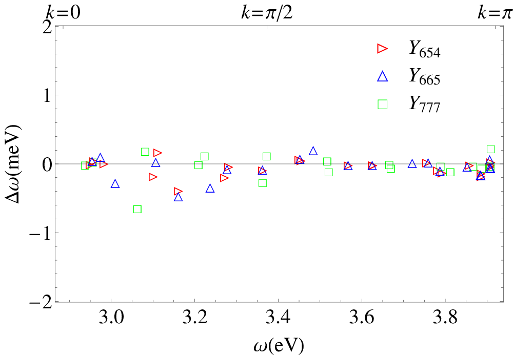
We further illustrate the above theoretical models using quantum-chemical calculations of branched polyfluorenes, a class of technologically important conjugated polymers [14, 15]. A Y-shaped family of molecules Yabc is shown in Fig. 3 (a), where , , and are the segment lengths in repeat units. The ground state molecular geometries were optimized at the AM1 level [16] with Gaussian09 package [17], followed by computing the vertical excitation energies and transition density matrices of up to 48 excited states using the Collective Electronic Oscillator (CEO) method [18, 19]. We select the first exciton band by checking the transition density matrices. Following our previous work [5, 4, 9, 7, 6] we further extracted the dispersion (Fig. 4 (a)) and scattering matrices for . For the scattering matrix of the terminal and of Y joint, we have and , where and are scattering phases of the -joint corresponding to a singlet and 2-fold degeneracy, respectively (see [9] for details). The scattering parameters in Fig. 4 allow for an accurate extraction of the excitation energies for an arbitrary Y-shaped molecules using the ES equation (14), see for example Fig. 3 (b).


From the scattering phases (Fig. 4 (b)), we extract the winding numbers and , the latter following from each having 2 kinks (sharp jumps) over half of the Brillouin zone, and a total shift of over the full Brillouin zone. Therefore, and according to Eq. (10), the number of solutions for the ES equation is
| (27) |
for the molecule Yabc shown in Fig. 3 (a). There are a total of 6 solutions for and , which do not correspond to physical states. Hence, the total number of states with excitation energies inside the exciton band is
| (28) |
where the factor arises due to time reversal symmetry, in full accordance with Eq. (12).
V Conclusion
In summary, we have identified an integer-valued topological invariant , associated with an arbitrary scattering center of a branched molecular structure (schematically represented by a graph), which is completely determined by the corresponding scattering matrix . The integer was motivated by a well known concept from algebraic topology, and has a simple integral form
| (29) |
We have reduced the problem of counting the number of solutions of the ES equations to an intersection problem, and further extended topological intersection theory to come up with a simple lower bound for in terms of the segment lengths and vertex winding numbers [Eq. (10)]. This allowed us to evaluate the total number of electronic excitations within a spectral region of a single exciton band [Eq. (2)]. Additionally, this permitted a simple and easy to interpret formula [Eq. (1)], that works for the generic case. Furthermore, it does not contain the band-edge indices , and counts the number of excitations in terms of the vertex topological charges . We also demonstrated that both lower bounds become exact for long enough linear segments. Quantum chemical calculations of Y-shaped branched oligofluorenes provide direct illustration of our theory. Being formulated in terms of dispersion relations and scattering matrices, the presented counting expressions are very general. Therefore, this approach can be applied to any quantum quasi-one-dimensional systems, or even more generally to any wave phenomena in networks, e.g., optical communications.
The introduced concepts carry a number of possible implications on studies of photo-physical phenomena in branched conjugated structures. The presented theory provides an explicit link between the graph topology (connectivity) of the branched system the interlining molecular electronic and optical properties defined by the spectrum of electronic excitations: The excited-state electronic structure in a finite molecule is a result of complex interplay between excitations in linear segments, determined by the exciton band structure in infinite polymers and electronic excitations in scattering centers. Chemical coupling between the linear segments and scattering centers modifies the excitations in the latter, resulting in bound and resonant states [8]. The resonant states that fall inside the exciton band show up as resonances in the density of states, or equivalently in sharp -rotations of the in the narrow regions of around the resonance of with a state at the scattering center, referred to as kinks [10, 8] are much harder to analyze, compared to bound states. Our counting result allows for a following interpretation: the number of resonant states in a finite structure is given by just the sum of the topological charges, associated with the scattering centers. In particular, when the connectivity of a conjugated structure is changed, with the scattering centers being kept the same, the resonant states do not appear or disappear, but rather their structure is modified. In the future we will study the dependence of the resonant states structure on the graph topology by examining the position dependent exciton density of states.
Finally, we note that the possible increase in the number of states inside the exciton band for shorter segments (i.e., in the case of inequality in Eq. (1)) can be explained by noting some of the bound states get “pushed” inside the exciton band due to the effects of quantum confinement of the exciton center of mass motion. We would like to emphasize that the inequality that forms a lower bound for [Eq. (1)], which follows from topological considerations, reflects a physical/chemical trend: Effects of quantum confinement of the exciton center of mass motion are sometimes turning the bound states into the resonant counterparts and not the other way around.
Acknowledgements.
This work is supported by the National Science Foundation under Grant No. CHE-1111350, and U.S. Department of Energy and Los Alamos LDRD funds. Los Alamos National Laboratory is operated by Los Alamos National Security, LLC, for the National Nuclear Security Administration of the U.S. Department of Energy under Contract No. DE-AC52-05NA25396. We acknowledge support of Center for Integrated Nanotechnology (CINT). We would also like to thank John Klein for helpful discussions regarding the index theorem.Appendix A Topological Properties of the Unitary Groups
In this appendix, we describe some relevant topological properties of the unitary groups in a simple and self-consistent fashion.
First, taking the determinant of a unitary matrix defines a map . We can define a map , referred to as a section, by defining to be a unitary matrix with the eigenvalues . Note that . A choice of a section defines an isomorphism (of topological spaces, as well as smooth manifolds, but not groups) , given by . We are interested in topological invariants of maps , or more precisely the homotopy equivalence classes of such maps. Since , a map is described by a pair of maps and . If denotes the set of homotopy classes of maps , then we have . Using the fact that consists of a single point, each -dimensional cycle in is contractible (meaning topologically equivalent to the constant map). As a topological space , so that , with the homotopy class of a map given by its winding number. Therefore , i.e., maps from a circle to a unitary group have exactly one topological invariant that takes values in the integers . This also implies that the determinant map generates an isomorphism . Formulated in a simpler way, to identify the topological invariant of a map one needs just to compute the winding number , where . Therefore, we refer to the topological invariant of a map as its winding number.
In proving the index theorem (see a sketch in Section III.3), we will make use of the fact that the space is contractible to a point. We reiterate that is a closed subspace of unitary matrices that have at least one unit eigenvalue. In particular, if a map misses , i.e., can be represented as a composition (where the second map is the inclusion), then . The contractibility can be demonstrated by presenting a continuous deformation (homotopy) of the identity map to a constant map, the latter mapping the whole domain to a single point. The spectra of matrices are contained in an open interval in the sense that the eigenvalues are given by with . Consider an obvious contraction of the interval to its center, given by the point . The contraction/deformation of the interval defines a corresponding contraction/deformation of the spectrum of any matrix . The described above deformation of the spectrum provides a deformation of the corresponding matrix: we deform the spectrum keeping the eigenspaces, related to the eigenvalues unchanged. This describes a contraction of to the point .
References
- [1] C. Wu, S. V. Malinin, S. Tretiak, and V. Y. Chernyak, Nature Phys. 2, 631 (2006).
- [2] C. Wu, S. V. Malinin, S. Tretiak, and V. Y. Chernyak, J. Chem. Phys. 129, 174111 (2008a).
- [3] Ibid, 174112.
- [4] Ibid, 174113.
- [5] C. Wu, S. V. Malinin, S. Tretiak, and V. Y. Chernyak, Phys. Rev. Lett. 100, 057405 (2008d).
- [6] H. Li, S. V. Malinin, S. Tretiak, and V. Y. Chernyak, J. Chem. Phys. 132, 124103 (2010b).
- [7] H. Li, C. Wu, S. V. Malinin, S. Tretiak, and V. Y. Chernyak, J. Phys. Chem. Lett. 1, 3396 (2010a).
- [8] H. Li, M. J. Catanzaro, S. Tretiak, and V. Y. Chernyak, J. Phys. Chem. Lett. 5, 641 (2014a).
- [9] H. Li, C. Wu, S. V. Malinin, S. Tretiak, and V. Y. Chernyak, J. Phys. Chem. B 115, 5465 (2011).
- [10] H. Li, S. V. Malinin, S. Tretiak, and V. Y. Chernyak, J. Chem. Phys. 139, 064109 (2013b).
- [11] E. Collini and G. D. Scholes, Science 323, 369 (2009).
- [12] G. D. Scholes and G. Rumbles, Nature Mat. 5, 683 (2006).
- [13] E. H. Spanier, Algebraic topology, Springer-Verlag, New York, 1981.
- [14] U. Scherf and E. J. W. List, Adv. Mater. 14, 477 (2002).
- [15] S. Becker, C. Ego, A. C. Grimsdale, E. J. W. List, D. Marsitzky, A. Pogantsch, S. Setayesh, G. Leising, and K. Mullen, Synth. Met. 125, 73 (2001).
- [16] M. J. S. Dewar, E. G. Zoebisch, E. F. Healy, and J. J. P. Stewart, J. Am. Chem. Soc. 107, 3902 (1985).
- [17] M. J. Frisch, G. W. Trucks, H. B. Schlegel, G. E. Scuseria, M. A. Robb, J. R. Cheeseman, G. Scalmani, V. Barone, B. Mennucci, G. A. Petersson, et al., Gaussian 09 Revision A.01, Gaussian Inc. Wallingford CT 2009.
- [18] S. Mukamel, S. Tretiak, T. Wagersreiter, and V. Chernyak, Science 277, 781 (1997).
- [19] S. Tretiak and S. Mukamel, Chem. Rev. 102, 3171 (2002).