Efficient Methods and Parallel Execution for Algorithm Sensitivity Analysis with Parameter Tuning on Microscopy Imaging Datasets
Abstract
Background: We describe an informatics framework for researchers and clinical investigators to efficiently perform parameter sensitivity analysis and auto-tuning for algorithms that segment and classify image features in a large dataset of high-resolution images. The computational cost of the sensitivity analysis process can be very high, because the process requires processing the input dataset several times to systemtically evaluate how output varies when input parameters are varied. Thus, high performance computing techniques are required to quickly execute the sensitivity analysis process.
Results: We carried out an empirical evaluation of the proposed method on high performance computing clusters with multi-core CPUs and co-processors (GPUs and Intel Xeon Phis). Our results show that (1) the framework achieves excellent scalability and efficiency on a high performance computing cluster – execution efficiency remained above 85% in all experiments; (2) the parameter auto-tuning methods are able to converge by visiting only a small fraction (0.0009%) of the search space with limited impact to the algorithm output (0.56% on average).
Conclusions: The sensitivity analysis framework provides a range of strategies for the efficient exploration of the parameter space, as well as multiple indexes to evaluate the effect of parameter modification to outputs or even correlation between parameters. Our work demonstrates the feasibility of performing sensitivity analyses, parameter studies, and auto-tuning with large datasets with the use of high-performance systems and techniques. The proposed techologies will enable the quatification of error estimations and output variations in these pipelines, which may be used in application specific ways to assess uncertainty of conclusions extracted from data generated by these image analysis pipelines.
Keywords:
Microscopy Imaging , Sensitivity Studies , Auto-tuning1 Background
We define algorithm sensitivity analysis as the process of comparing results from multiple analyses of a dataset using variations of an analysis workflow (e.g., different input parameters or different algorithm versions) and quantifying differences in the results. This process is executed in many phases of scientific research, including validation of models, parameter studies and error estimation. In validation and error estimation, comparison of multiple analyses can be used to quantify and evaluate how much models differ or agree, and differences among output from different models can be combined in application specific ways to assess errors and uncertainty in output. Application parameter tuning is another important task in sensitivity analysis. In this task, the parameter space of an analysis workflow is searched by comparing analysis results with ground truth to find the set of parameters which produces results that are closest to the ground truth with respect to some comparison metric.
1.1 Motivation
The primary motivation for our work is to support large scale biomedical imaging studies, in particular those working with large numbers of whole slide tissue images. High-resolution microscopy imaging of tissue specimens enables the study of disease at the cellular and sub-cellular levels. Characterizing the sub-cellular morphology of tissue can lead to a better understanding of disease mechanisms and a better assessment of response to treatment. It is increasingly becoming feasible, with wider availability of advanced tissue scanners at lower price points, for research studies to collect tens of thousands of high resolution images. A contemporary digital microscopy scanner can capture a whole slide tissue image containing 20 billion pixels (using 40X objective magnification) in a few minutes. A scanner with a slide loader and auto-focusing mechanism can generate hundreds of images in one or two days [1].
| Parameter | Description | Range Value |
| Target Image | Image used as a normalization target | TI |
| B/G/R | Background detection thresholds | B, G, R |
| T1/T2 | Red blood cell detection thresholds | T1,T2 |
| G1/G2 | Thresholds to identify candidate nuclei | G1 |
| G2 | ||
| MinSize | Filter out objects with area (pixels) | MinSize |
| MinSize after candidate nuclei identification | ||
| MaxSize | Filter out objects with area larger than | MaxSize |
| MaxSize after candidate nuclei identification | ||
| MinSizePl | Filter out objects with area smaller than | MinSizePl |
| MinSizePl before watershed is executed | ||
| MinSizeSeg | Filter out nuclei with area smaller than | MinSizeSeg |
| MinSizeSeg from final segmentation | ||
| MaxSizeSeg | Filter out nuclei with area smaller than | MaxSizeSeg |
| MaxSizeSeg from final segmentation | ||
| FillHoles Structure | Structure of the propagation neighborhood | FillHoles -conn-conn |
| MorphRecon Structure | Structure of the propagation neighborhood | MorphRecon -conn-conn |
| Watershed Structure | Structure of the propagation neighborhood | Watershed -conn-conn |
| Parameter | Description | Range Value |
|---|---|---|
| Target Image | Image used as a normalization target | TI |
| OTSU | Weighting value applied to the OTSU threshold value | OTSU |
| Curvature Weight | Curvature weight (CW) of the level set functions | CW |
| MinSize | Minimum object size in micron per dimension | MinSize |
| MaxSize | Maximum object size in micron per dimension | MaxSize |
| MsKernel | Spatial radius used in the Mean-Shift calculation | MsKernel |
| LevetSetIt | Number of iterations of the level set computation | LevetSetIt |


Analysis of tissue images involves extraction of salient information from the images in the form of segmented objects (e.g., nuclei or cells) and their size, shape, intensity and texture features. These features are then used to develop morphological models of the specimens under study to gain new insights. A typical analysis workflow consists of normalization, segmentation, feature computation, feature refinement and classification operations. The first three analysis stages are typically the most computationally expensive phases of an analysis run. Figure 1 presents two analysis workflows used in this work. These workflows share the same high level structure, but implement the segmentation stage using different strategies. The first (Figure 1) uses morphological operations and watershed in the segmentation [2], whereas the second (Figure 1) performs the segmentation based on level set and mean shift clustering [3, 4]. The cascade of operations employed by each of the workflows are presented in the figures.
Most image analysis workflows are sensitive to variations in input parameters. A workflow optimized for a group of images or a type of tissue may not perform well for other tissue types or images. For instance, accurate segmentation of cancer nuclei is an important image analysis task in digital pathology. Boundaries of segmented nuclei are algorithm dependent. Input parameters, such as the choice of methods for seed selection, intensity thresholds for boundary detection and thresholds for separation of clumped nuclei, will impact the results (the number and locations of detected nuclei, the shape of boundaries of a nucleus, etc). Figure 2 shows nuclear segmentation results from two analysis runs. The two analysis pipelines have good agreement in some regions (i.e., the boundaries of the polygons overlap closely) and large disagreement in other regions, where either one algorithm has not segmented nuclei while the other has or there are large differences between the boundaries of a nucleus segmented by the two algorithms.

It is, therefore, important to quantify the impact of changes in input parameters to output generated by different stages and by the overall workflow. In this work, we focus on the segmentation stage as our example, because this is a crucial stage in extracting morphological information from images and consists of several complex and parameterized data transformation steps. An approach for evaluating sensitivity of an analysis workflow and tuning its parameters is for the user to manually run the workflow on small patches of images, visually evaluate the results, modify the workflow parameters, and repeat the process until a satisfactory set of parameters is obtained [5, 6].
1.2 Data and Computation Challenges
This labor-intensive and error-prone process does not scale to multiple workflows and large sets of images. About 400,000 nuclei are identified in a WSI, and this segmentation process takes at least an hour on a single CPU-core. A parameter analysis run may require the evaluation of hundreds or thousands points (parameter combinations), and each of them correspond to a full run of the analyses pipelines on the input data. As such, for instance, the execution of a sensitivity analysis study involving the evaluation of 2,000 points in the application parameter space (application run) with 55 WSIs (The Cancer Genome Atlas (TCGA) contains over 30,000 WSIs) would take about 18 years in a single CPU-core and would read/stage close to 830 TB of data.
It is, thus, challenging to carry out parameter sensitivity analysis and auto-tuning, even for the segmentation stage, because (i) the number of possible parameter combinations of an analysis workflow is staggeringly high. Table 2(b) presents the parameters of interest in the segmentation stage for our two use case image analysis workflows. The space of parameter values only for the segmentation stage for the watershed and level set based workflows contain, respectively, over 21 trillion and 2.8 billion points; (ii) the execution of a single parameter combination may be computationally very demanding depending on the input dataset. This is critical in the context of whole slide tissue image analysis, because the execution of a single analysis run (i.e., the evaluation of a single point in the parameter space) can take hours or days depending on the size of the input dataset.
1.3 Contributions of Our Work
The data and computation challenges of image analyses and sensitivity studies are major roadblocks to taking full advantage of advanced imaging technologies and tissue specimens. To make sensitivity analyses feasible, it is necessary: (i) to propose and utilize effective sensitivity analysis and auto-tuning methods; and (ii) to leverage high performance computing techniques to accelerate these analyses. Our approach addresses these challenges by a framework that integrates the following components:
Efficient Sensitivity Analysis (SA) Methods: Sensitivity analysis methods and techniques allow for the user to understand and quantify variability in the output of a model, and apportion those variabilities to source of uncertainty in the input parameters. It may be useful in several tasks, which include understanding the output ranges, remove parameters that have little influence from other studies etc. In this work, we propose to use a number of global SA techniques to study sensitivity analysis in the output of microscopy image analysis applications. They include Morris One-At-A-Time design (MOAT) [7, 8, 9, 10], design experiments with pseudo-random parameter probe to calculate importance metrics [11, 12], such as Pearson and Spearman’s correlation coefficients, and Variance-based Decomposition (VBD) [13, 14].
Efficient Parameter Auto-tuning Methods: We also study input parameter tuning for the same class of applications. In this task the input parameters of an analysis application are systematically varied, and analysis results from input parameter sets are compared to a reference result. Comparison outcome is used to adjust the parameter set and repeat the process. The goal is to search the application parameter space and find parameters that produce good results with respect to a domain specific metric.
On-the-fly Spatial Comparative Analysis Tools. This component of our solution deals with the computation of metrics of interest that involve the comparison of spatial objects from segmented images. It provides a query-based interface to the user, and is built on top of a set of core operations such as cross-matching, overlay of objects, spatial proximity computations between objects, and global spatial pattern discoveries. These core operations are combined to implement metrics that include Dice Coefficient, Jaccard Coefficient, Intersection Overlapping Area, Non-Overlapping Area (Number of pixels differently segmented) [15]. K-Nearest Neighbor queries are also support, and can be use to select a subset of objects of interest (e.g., close to region of study as a vein), which may be further passed for computing the other quantitative metrics. This functionality is built on our runtime system to allow for those metrics to be computed on-the-fly as objects are identified by segmentation algorithms. It allows for an efficient execution as the entire process is computed online without having to go through the expensive step of loading the data in a spatial database [16].
Scalable Runtime for Execution of Sensitivity Analysis and Auto-tuning Processes. We have developed a framework that aims to address the processing and data management challenges of the image analysis pipelines execution through runtime optimizations targeted at distributed memory systems with hybrid multi-core CPU and co-processors and multiple levels of storage. In this part of the work, we have optimized the analysis pipelines by (1) parallelizing core operations of image analysis for CPU and the Intel Xeon Phi coprocessors [17] and (2) developing scheduling strategies that can appropriately map computations to heterogeneous processors. We also proposed optimizations targeting specific aspects of parameter analysis and auto-tuning studies. They include efficient data movement and staging, data-aware assignment of stages and operations in an analysis workflow that exploits that optimize the system for repeated execution of workflows with different parameters that process the same datasets. Also, we propose an approach to reduce the computation costs in these analyses through the simultaneous parameter evaluation in order to eliminate common computations in the execution of an application with multiple parameter sets.
2 Materials and Methods
Figure 3 shows how sensitivity analysis and parameter auto-tuning processes are carried out. The user specifies the set of input images, an image analysis workflow, input parameters to the image analysis workflow, and the metric of interest (e.g., Dice) for comparison of image analysis results. The image analysis workflow is executed using a scalable runtime environment, called Region Templates, on a high performance machine, while the input parameters are systematically varied by sensitivity analysis and auto-tuning methods supported by our framework. When image analysis results, i.e., sets of segmented objects, are produced, the results are processed by the spatial comparative analysis component. The segmentation results are compared to a reference segmentation dataset. The reference segmentation dataset may, for instance, be a previously computed set of results from earlier sensitivity analysis runs or a set of manual segmentation results, if the goal of sensitivity analysis is to tune analysis parameters to match the manual segmentation results. The comparison metric value generated by the comparative analysis component is then used as an error metric by the sensitivity analysis and auto-tuning methods which compute the next set of input parameters. This process is repeated until the required set of parameters is covered (in the case of sensitivity analysis) or error between the analysis results and the reference dataset is below a threshold (in the case of parameter auto-tuning).

2.1 Sensitivity Analysis (SA) Methods
Sensitivity Analysis (SA) is may be local or global, but in either case the methods evaluate the variance in the output with respect to input parameter changes. Local analysis focuses on measuring sensitivity in the neighborhood of a specific point in the parameter space. Global SA, which is implemented in this work, examines sensitivity output from the perspective of whole range of parameter variations [9]. A SA study includes selecting uncertainty input factors and the application output of interest, running the application with a number of points defined by a SA method, and the actual calculation the sensitivity statistics. Several SA methods can be employed in a study. SA methods fall into one of two types [9]: methods that are used for an initial fast exploration and are used in practice to quickly screen non-influential input parameters that may be removed from further analysis; and methods that compute measures of importance or quantitative sensitivity indices. We implement methods from these two types in our framework as described below.
2.1.1 Methods to Screen Input Parameters
Our current implementation supports one of the most commonly used screening methods, called Morris One-At-A-Time (MOAT) design [7], in which each input parameter is perturbed along as discretized input space while fixing others. In the MOAT, the -dimensional input space (for parameters) is partitioned uniformly in levels, creating a grid with points in which the model evaluations take place. Each perturbation of an input parameter creates a parameter elementary effect computed as shown in Equation 1.
| (1) |
where y(x) is the image analysis output metric value before the perturbation. In our case, the output refers to the metric of interest calculated comparing the application output mask to a reference mask. The reference mask set, in these analyses, was calculated using the application default parameters. Therefore, we will evaluate how the changes in the input parameters reflect in mask changes that are computed using different spatial metrics of interest that compare masks using a fixed pre-computed mask set as a reference. To account for global SA, the value is typically large. This implementation uses that leads to steps slightly larger that half of the input range for input variables scaled between 0 and 1.
The distribution of elementary effects of the input space characterizes the effects on the output, which are measured using mean (), modified mean (), and standard deviation () of elementary effects for each input parameter [8]. The mean and modified mean represent the effects of the input on the output, whereas the standard deviation reveals nonlinear effects. This analysis involve application runs (or evaluations in the input parameter space), and value is suggested to be on the range of 5 to 15 [9, 10]. The MOAT does not produce information about interactions of parameters, but gives evidence of their existence.
2.1.2 Methods to Compute Importance Measures
These methods provide quantitative measurements of the correlations between input parameters and application output or different input parameters through correlation coefficients. If a sample of application runs for a set of input values and the respective output measures are available, a linear model could be fit on the sample to try explaining it. Some of the coefficients that we compute out of these analyses include Pearson’s correlation coefficient (CC) and partial (PCC) correlation coefficient as well as Spearman’s rank correlation coefficient (RCC) and partial rank correlation coefficient (PRCC) . The simple and partial correlation coefficients are similar, but the latter excludes effects from other parameters or variables. When the variables are orthogonal, the simple and partial correlations are the same, whereas the ranked correlations are helpful when the relationship between parameters are non-linear [18].
The CC for and is calculated as: , where and could be two parameters, a parameter and the output, etc. The output here is calculated similarly to that described in the previous section. A pre-computed mask set is used as a reference, and the resulting mask set for a set of input parameters is compared to the reference set and the output of the comparative analysis is taken as the result of the application of that particular parameter set. The Spearman’s correlation is similar to the Pearson’s, except that it is calculated based on ranked data [11]. The application runs or sample used to calculate these metrics is typically generated from a probabilistic exploration of the parameter space. We support a number of stochastic methods to perform the exploration, such as the commonly used Monte Carlo (random) sampling and Latin hypercube sampling(LHS). The LHS have been shown to achieve better accuracy in parameter sensitivity studies [12].
Our implementation also supports the Variance-based Decomposition (VBD) global sensitivity method. VBD splits output uncertainty effects among individual or groups of parameters [13] and can account for non-linear relationships among them. VBD computes the “main effect” sensitivity index [14] and the “total effects” sensitivity index [19]. The measures the amount of the output variance that can be attributed to parameter alone (first-order effects). If the sum of the values is close to one, most of the output variance is explained by single parameter effects. The total effect index measures the first-order and higher-order effect due to interaction with other parameters. The possible number of higher-order effects grows exponentially with the number of input parameters. Therefore, in practice, it is not viable to account for interactions of order higher than two. The VBD is very compute intensive with respect to sampling, since for input parameters and samples, it requires application runs, and reasonably accurate indices require to be in the other of hundreds or thousands. Those indices are computed here as described in [13].
2.2 Parameter Auto-tuning Algorithms
The auto-tuning execution flow (presented in Figure 3) is similar to that of parameter study. The auto-tuning algorithm selects one or more sets of application parameter values. The image analysis application is executed for those parameter sets to compute the metric of interest against a reference dataset (e.g., an image segmentation mask annotated by a pathologist). The metric output for each parameter set is fed back to the auto-tuning algorithm, which computes another set(s) of parameters to be evaluated. This iterative process continues until one of the two supported stop conditions is met: (i) maximum number of iterations or (ii) a given metric threshold value is reached.
The current implementation supports the following auto-tuning algorithms: Nelder-Mead simplex (NM) [20], Parallel Rank Order (PRO) [20], and a Genetic Algorithm (GA) [21]. The NM and PRO approaches have been implemented using Active Harmony (AH) [20, 22], whereas the GA has been developed by us. Active Harmony is an auto-tuning system that is primarily designed and employed for tuning application runtime performance. In our work, we make a novel use of Active Harmony for searching parameter space to improve application analysis results. All algorithms try to minimize (or maximize by negation) an unknown function by probing and exploring the parameter search space.
The Nelder-Mead method uses a simplex or polytope of vertices in a k-dimensional search space. The simplex is updated in each iteration by removing the vertex with the worst value (), which is replaced with a new vertex which has a lower function value. This operation involves computing the centroid of the remaining simplex vertices to replace with a point on line . Typical values are 0.5, 2, and 3. The values of define whether the transformation on the simplex is a reflection (), an expansion (), or a contraction (). The Nelder-Mead method usually performs a reflection first and, depending on the results, follows the reflection with a expansion or contraction. The original method has been modified in Active Harmony to deal with non-continuous search spaces.
The Parallel Rank Order (PRO) algorithm uses a set of K points from a simplex (K N + 1) for a N-dimensional space. Each iteration of the algorithm calculates up to new vertices, which are computed by a reflection, expansion, and shrinking of the simplex around its vertex with the optimal value. Multiple vertices generated during each iteration may be evaluated independently. This feature enables concurrent execution of multiple copies of the application with different parameter sets (vertices) on a high performance machine. The reflection step succeeds if at least one of the evaluated vertices lead to an improvement of the optimization results. If no point succeeds during reflection, the simplex shrinks around the best vertex. The expansion check follows a successful reflection and is executed to accept the simplex or not. The simplex is expanded when accepted. Search continues with a new iteration. The algorithm stops when it converges to a point in the search space or after a number of iterations have been executed.
The Genetic Algorithm (GA) [21] models points in the search space (parameter values) such that each parameter corresponds to a gene of an individual. The initial population in our implementation is created by randomly selecting parameter values from the search space. The population is evolved through reproduction (selection), crossover and mutation. The selection phase retrieves a percentage of the individuals with the best fitness (i.e., the best results with respect to our optimization function) that are duplicated to replace the ones with the worst fitness. In the crossover phase, the individuals are grouped into pairs, and all genes with an index higher than a certain value are swapped between the individuals. This index value is randomly selected for each pair of individuals. Finally, each individual may suffer mutation of its genes. In this case the new value for a gene is randomly selected. After these phases, the new population is evaluated via a fitness function [21] (metric of interest). The outcome of the evaluation is input back to the algorithm to build another generation. The process continues until a preset number of generations (iterations) is reached. As a performance optimization, multiple individuals from a generation can be evaluated concurrently.
Most prior works on the problem of parameter estimation or optimization in imaging segmentation employ techniques for specific segmentation models. A pseudo-likelihood is used in [23] to estimate parameters for a conditional random field based algorithm. Graph cuts are employed to compute maximum margin efficient learning in segmentation parameters [24]. A non-convex function is optimized in [25, 26] with techniques to avoid sensitivity in segmentation due to the initial parameter choices. Open-Box [6] is another interesting solution that is specific to segmentation algorithms based on spectral clustering. It deals with the optimization by exposing key components of the segmentation to the user. The Tuner system [5] deals with general segmentation algorithms and focuses on creating statistical models from sampling runs that describe the segmentation response function, and employs a Gaussian process model to explore the parameter space. The areas of the search space identified as promising are further explored to refine the parameters. In our work, we treat the segmentation algorithm as a black-box. Additionally, instead of using a statistical model that describes the application, we employ efficient optimization algorithms that can quickly converge to desired results. Our solution also allows for the use of multiple auto-tuning algorithms. We employ HPC with several optimizations to accelerate application runs in the parameter tuning phase. We provide to the user several domain specific metrics for evaluating algorithm outputs, and new metrics can be incorporated via a spatial querying engine.
2.3 Scalable Execution of Sensitivity Analysis and Auto-tuning on Parallel Machines
Sensitivity analysis and parameter auto-tuning are extremely time consuming processes, because computationally expensive analysis pipelines have to be executed multiple times on large volumes of imaging data. They can benefit from high performance computing (HPC) systems that have hybrid computation nodes equipped with accelerators (GPUs and Intel Xeon Phi co-processors) and multiple levels of data storage consisting of GPU and CPU memories, SSDs, local spinning disks. The use of hybrid systems equipped with CPU and accelerators is a fast growing topic that has attracted attention for research in are as compiler techniques, scheduling, runtime systems, and parallelization of applications [27, 28, 29, 30, 31, 32, 33, 34, 35, 36, 17, 37]. In special, several Biomedical Informatics applications and research initiatives are able to benefit from accelerators and parallel HPC systems [38, 30, 39, 40, 41, 42, 43, 44, 45, 46, 47, 48, 49, 50, 51]. In this work, we have implemented support for sensitivity analysis and parameter auto-tuning on the region templates (RT) runtime system [52] to address the computational requirements of these processes on HPC systems with co-processors. The region templates runtime system provides core functions for scheduling of application operations across multiple computation nodes and on co-processors (such as CPUs and Intel Xeon Phis) and manages data movement across multiple storage layers.
The processing structure of a region template application is expressed as a hierarchical dataflow graph. That is, an operation itself can be composed of lower-level operations organized into another dataflow. Application workflows are decomposed into components of computation that consume, transform, and produce region template data objects instead of reading/writing binary data directly from/to other tasks or disk. The region template data abstraction provides a generic container template for common data structures, such as pixels, points, arrays (e.g., images or 3D volumes), segmented and annotated objects and regions, that are defined in a spatial and temporal domain. Using these containers, the application developer can avoid having to manually deal with communication of data structures accross memory hierachies of nodes in a distributed machine.

Figure 4 presents the main components of the region template framework: the region templates data abstraction, the runtime environment, and the hierarchical data storage layer. The runtime environment deals with the instantiation of components for execution with nodes of a distributed memory environment and interacts with the data storage layer for data region management. The storage layer is responsible for exploiting the memory hierarchy in a distributed memory system to efficiently move region template data among nodes. The runtime environment of RT implements a Manager-Worker execution model that combines a bag-of-tasks execution with the dataflow pattern. The application Manager creates instances of coarse-grain stages, which include input data regions, and exports the dependencies between the stage instances. The assignment of work from the Manager to Worker nodes is performed at the granularity of a stage instance using a demand-driven mechanism. Each Worker may execute several stage instances concurrently to take advantage of multiple computing devices (CPUs and co-processors) on a computation node. Computing devices on a node are used cooperatively by dispatching fine-grain tasks for execution on a CPU core or a co-processor (e.g., an Intel Phi or a GPU) via a performance-aware task scheduling (PATS) algorithm [53, 54]. PATS assigns tasks to a CPU core or an accelerator based on the tasks estimated acceleration on each device and on the device load. We refer the reader to our earlier publication [52] for details of the region templates framework and runtime environment. In this paper we describe two optimizations in the region templates framework that target the requirements of the sensitivity study and parameter tuning processes. The first one is a new hierarchical data storage layer, which improves data locality for this class of application (Section 2.3.1). The second optimization is a strategy to avoid re-computation overheads during the evaluation of multiple parameter sets for the same workflow (Section 2.3.2).
2.3.1 Storage Management and Optimizations
The same or overlapping sets of data elements in one or more stages of the analysis workflow are processed and re-processed as input parameters are varied in an algorithm sensitivity analysis run. To take advantage of this, we have developed a new hierarchical storage infrastructure for RT and a strategy that considers data locality during the scheduling of application stage instances to improve the effectiveness of maintaining data in faster memory for reuse. The data storage layer is built as a distributed data management infrastructure, which can use an arbitrary number of memory layers within a node and across a distributed memory system. It is implemented as a module of the Worker processes in the runtime system. The memory/storage hierarchy of the target system is defined in a configuration file. The configuration file includes the number of storage levels used, the position of each storage in the hierarchy and a description of each level: type of storage device (e.g., RAM, SSD, HDD, etc), storage capacity, path for storing data, and storage visibility (local or global). Storage specified as local can only be directly accessed within the node (Worker process); Data regions associated with local storage are not directly visible to other nodes (Workers). Storage specified as global is visible to other nodes and is used to exchange data among stages of a region templates application.
The data storage layer is in charge of storing and retrieving instances of region templates. The runtime system contacts the data storage layer whenever a region template instance is output or requested by an application stage or operation. When accessing a region template instance, the search for the requested data may result in three cases: (i) The data is found in a local storage component; it is directly returned to the application stage/operation. (ii) The data is found in global storage; it is retrieved and transferred by the storage layer to the requesting node and application stage/operation. (iii) The data is found neither in local storage on the requesting node nor in global storage. This means the data is stored in local storage of the node in which it was produced (the source node). Inter-processor communication is necessary with the source node to move the data to a storage component of global visibility, before the data can be retrieved.
Data regions are staged to the data storage layer automatically. The runtime system iterates through data regions generated and used by an application operation and inserts those marked as output to the storage layer. The insertion is always performed into the highest (i.e., the fastest) level of the storage hierarchy with enough capacity to save the data regions. When a level reaches its maximum storage capacity, a cache replacement strategy is employed to select data regions that should be moved to a lower level in the hierarchy. Each level of a storage hierarchy may use one of the supported data replacement policies: First-In, First-Out (FIFO) and Least Recently Used (LRU). New policies can be incorporated via the application programming interface.
Data should ideally be reused or retrieved when it resides in faster memory/storage layers. In order to reduce data access costs, we have developed a data locality-aware scheduling (DLAS) approach that considers the location of data to be accessed when scheduling and mapping application stages and operations to the nodes of the computation system.
The DLAS strategy is implemented at the Manager level of the runtime system. With this policy, when the notification is received that a given application stage instance (referred to as the original stage instance) has finished, the Manager takes into account the locality of the data produced by that stage instance to determine the node in which stage instances that use the produced data should be executed. In this process, DLAS calculates the amount of data reuse of stage instances that consume data from the original stage instance, and inserts them into a queue of preferred stage instances for execution in the Worker node that executed the original stage instance. A queue of preferred instances is maintained for each Worker in decreasing order of the amount of expected data reuse. When a Worker requests a stage instance for execution, the Manager will try to assign the stage instance that reuses the maximum amount of data — that is, the stage instance on the top of the queue for the requesting Worker. If the queue is empty or none of the stage instances in the queue have dependencies resolved (i.e., they cannot be scheduled for execution), an instance is chosen using the First-Come, First-Served (FCFS) order among those stage instances ready for execution.
2.3.2 Optimized Simultaneous Parameter Evaluation
The execution of parameter study and auto-tuning algorithms (PRO and GA) allows for multiple simultaneous parameter set executions and evaluations per iteration of the process (Figure 3). We exploit this characteristic to optimize the evaluation of these multiple runs with different parameter values. Instead of replicating the segmentation/application workflow for each parameter set to be evaluated, we created a strategy that merges and eliminates replicas of common computation paths of the workflows for faster evaluation of multiple parameters in each iteration.

Figure 5 shows two schemes for instantiating an application workflow in a parameter analysis study in which multiple parameter sets are tested in an iteration. The replica based scheme instantiates the entire application workflow for each parameter set and dispatches multiple independent workflow instances for execution. The compact composition scheme, on the other hand, merges the instances of an application workflow into a single, compact workflow graph to reuse common stages in the separate workflow instances. The compact workflow graph representation draws from a data structure called FP-Tree [55]. The FP-tree represents sets of transactions in a structure in which common parts of transactions are expressed in a single path on the structure. In our case, we want to merge multiple workflows to create another workflow in which common computations from multiple parameters are eliminated. The common computations are found in stages that have the same parameters and input data in multiple workflows.
The construction of the compact representation is presented in Algorithm 1. To simplify the presentation of the algorithm, we assume that both the compact graph (comGraph) and each instance of the application graph (appGraphInst) to be merged have a single start root node. The algorithm takes the application workflow graph (appGraph) and parameter sets to be tested simultaneously as input (parSets) and outputs the compact graph (comGraph). It iterates over each parameter set (lines 3-5) to instantiate a replica of the application workflow graph with parameters from . It then calls MergeGraph to merge the replica to the compact representation.
The MergeGraph procedure walks simultaneously in an application workflow graph instance and in the compact representation. If a path in the application workflow graph instance is not found in the latter, it is added to the compact graph. The MergeGraph procedure receives the current set of vertices in the application workflow (appVer) and in the compact graph (comVer) as a parameter and, for each child vertex of the appVer, finds a corresponding vertex in the children of comVer. Each vertex in the graph has a property called deps, which refers to its number of dependencies. The find step considers the name of a stage and the parameters used by the stage. If a vertex is found, the path already exists, and the same procedure is called recursively to merge sub-graphs starting with the matched vertices (lines 8-9). When a corresponding vertex is not found in the compact graph, there are two cases to be considered (lines 10-23). In the first one, the searched node does not exist in comGraph. The node is created and added to the compact graph (lines 11-17). To check if this is the case, the algorithm verifies if the node () has not been already created and added to comGraph as a result of processing another path of the application workflow that leads to . This occurs for nodes with multiple dependencies, e.g., D in Figure 5. If the path (A,B,D) is first merged to the compact graph, when C is processed, it should not create another instance of D. Instead, the existing one should be added to the children list as the algorithm does in the second case (lines 19-23). The PendingVer data structure is used as a look-up table to store such nodes with multiple dependencies during graph merging.
In the proposed algorithm, application workflows are expected to be directed graphs. If a stage is used multiple times in the same application, it is necessary to rename the repeated stage to prevent the algorithm from finding incorrect nodes in the look-up of pending nodes (line 11).
2.3.3 Spatial Comparison Support
We have implemented a comparative analysis module in the region templates system for efficient quantitative comparison of multiple segmentation results using a query-based interface. By performing comparison of objects from multiple image segmentation results using a set of core operations that include spatial cross-matching, overlay of objects, spatial proximity computations between objects, and global spatial pattern discoveries, we are able to compute a number of metrics of interest from objects detected in segmentation runs that are used in algorithm sensitivity analysis. The metrics we built in region templates using this module include: Dice Coefficient, Jaccard Coefficient, Intersection Overlapping Area, Non-Overlapping Area (Number of pixels differently segmented) [15]. However, the core operations previously described can be combined in a number of ways to create a more extensive set of metrics. Also, we support more complex queries that include spatial proximity computations between objects using Nearest Neighbor Queries (KNN), which may be combined with any other metric of interest to investigate the characteristics of a subset of objects close to another object of interest (e.g, cells close to a vein or other structure). These features are available with region templates through its integration with a GIS querying framework [16, 56]. In order to use it in an application, the user simply connects an existing application stage (component) developed in RT to her application, passing the masks that need to be compared to this component.

The overall view of the metric computation flow is presented in Figure 6. The RT application computes a mask and passes the computed mask and any other reference mask as input to the comparative analysis module, which as described is instantiated in the distributed environment an application stage. In order to execute spatial queries, the Comparative Analysis module extracts the objects (cells, veins, etc) from the masks and convert them into polygons. After this process, an application running under Region Templates Framework can use one of the supported queries to perform spatial processing. The implemented queries can use the core capabilities of the Hadoop-GIS Framework [16] to calculate the intersection area between the two sets or calculate their spatial proximity. After receiving the results from the spatial processing engine, the Comparative Analyses module may calculate the Dice Coefficient, Jaccard Index or some other metric in order to complete the query task.
The actual spatial queries are computed using provided Hilbert R*-Tree indexing-driven spatial query engine, which is critical to quickly identify overlapping objects in join based operations [57]. First, a R*-Tree is built from objects minimum bounding boxes in each mask, and a spatial filtering operation is performed to identify possibly overlapping objects (those with intersecting bounding boxes), which are refined to those that overlap. This set is passed to a final phase in which actual operations performed to compute spatial measurements results. These results may be the overlapping area of the intersection, the area of the union of the polygons etc. A detailed explanation of the coefficients we calculate is provide bellow:
Dice Coefficient or The Sørensen-Dice index [58, 59]
This coefficient ranges from 0 to 1 and is used to measure the similarity of two samples. This metric can be calculated by dividing twice the intersection area of two samples by the sum of their respective areas.
Jaccard Index Metric
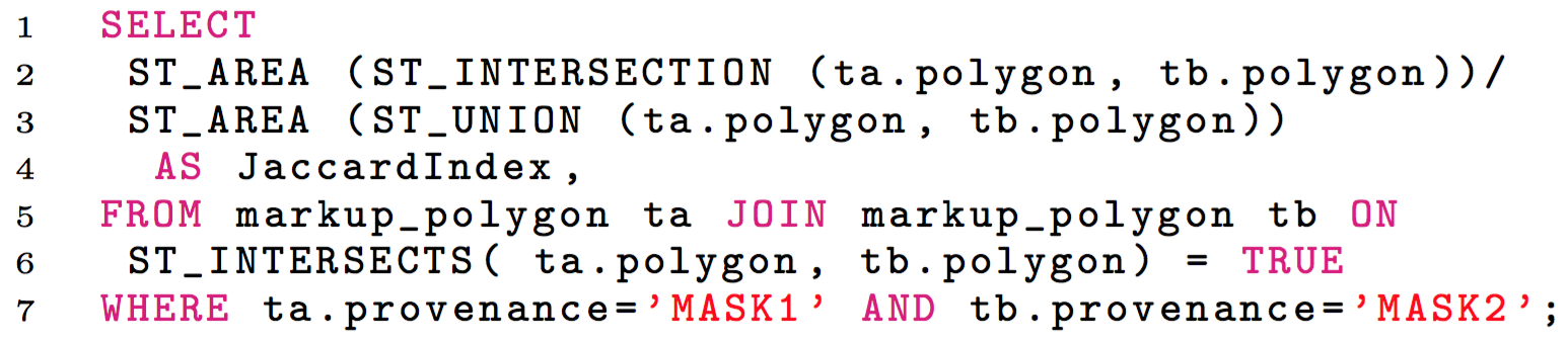
it also ranges from 0 to 1 and is similar to the Dice Coefficient. The Jaccard Index is calculated by dividing the intersection area between two sets by the union area of these sets [60]. The SQL expression equivalent to this metric is shown in Figure 7.
Intersection Overlap Area Metric
This metric represents the relation between the total area of the intersection between two masks divided by the area of reference mask set.
Nearest Neighbor Query
Nearest neighbor (KNN) search in analytical imaging analysis can be computationally expensive, we use Hadoop-GIS to efficiently perform these queries in order to understand correlations between spatial proximity and cell features. The implemented query allows selecting the K-nearest objects or within a certain bound. A typical scenario that a application can take advantage of this query is to find the nearest objects (blood vessels, cells, etc) for each cell of a given set in order to study their characteristics and correlations.
3 Results and Discussion
We have evaluated the proposed methods and optimizations using a set of Glioblastoma brain tumor tissue images collected in brain cancer studies [2]. The images were divided into 4K4K tiles; each tile was processed concurrently with other tiles in a bag-of-tasks style execution. The image analysis workflow consisted of normalization, segmentation and comparison stages. The comparison stage computes the difference between masks generated by the application and the reference data for each set of parameters. The experimental evaluations were conducted on two distributed memory machines. The first one is the TACC Stampede clusterhas a dual socket Intel Xeon E5-2680 processors, an Intel Xeon Phi SE10P co-processor and 32GB RAM. The nodes are inter-connected via Mellanox FDR Infiniband switches. The second cluster, called Eagle, is a small cluster at Stony Brook University with 10 computing nodes. Each node has dual socket Intel Xeon E5-2660 processors, an Intel Phi 5110P co-processor, 256GB RAM, 1TB spinning disk and a 512GB SSD. Stampede uses a Lustre file system accessible from any node, while each node on Eagle has a local Linux file system. The application and middleware codes were compiled using Intel Compiler 13.1 with “-O3” flag. The MIC operations used the offload mode – a computing core was reserved to run the offload daemon and at most 240 threads were launched.
3.1 Sensitivity Analysis
3.1.1 Finding Important Parameters with MOAT
The use-case microscopy image analysis workflows employed in this study have k=15 and k=7 parameters (described in Table 2(b)), which we first study using MOAT in order to try pruning the parameter space before more costly analyses such as VBD and tuning are employed. Thus, in this phase, we use the MOAT design to select the most impacting parameters to be used in downstream analyses. The output of the applications to the MOAT method is the difference in number of pixels from the mask computed with parameter values selected by the method and a mask precomputed using the application default parameter values. The watershed based workflow employs 55 Glioblastoma brain tumor WSIs (4,276 4K4K non-background only image tiles) and the level set based is evaluated with 1 Glioblastoma brain tumor WSI (71 4K4K that were partitioned into 512512 tiles). A smaller dataset is used with the level set workflow because it is more compute demanding.
We have considered parameter space partition with 20 levels for each of the parameters in Table 2(b). The number of executions of the image analysis workflow for the entire input dataset value is calculated as . The experiments were performed using 128 nodes of the Stampede cluster and they 15681s and 6825s, respectively for the watershed and level set workflows when r is 15.
| Parameter | r = 5 | r=10 | r=15 | |||
|---|---|---|---|---|---|---|
| 1 (Blue) | 4.59E+04 | 1.03E+05 | 2.30E+04 | 7.26E+04 | 2.77E+04 | 7.87E+04 |
| 2 (Green) | 3.50E+04 | 7.83E+04 | 3.89E+04 | 9.20E+04 | 2.59E+04 | 7.38E+04 |
| 3 (Red) | 0.00E+00 | 0.00E+00 | 0.00E+00 | 0.00E+00 | 0.00E+00 | 0.00E+00 |
| 4 (T1) | 5.90E+05 | 9.01E+05 | 1.46E+07 | 4.24E+07 | 2.01E+07 | 4.15E+07 |
| 5 (T2) | 7.10E+07 | 1.24E+08 | 4.63E+07 | 9.42E+07 | 5.46E+07 | 9.08E+07 |
| 6 (G1) | 3.78E+08 | 5.87E+08 | 1.10E+09 | 2.25E+09 | 9.35E+08 | 1.93E+09 |
| 7 (G2) | 3.08E+09 | 3.67E+09 | 2.38E+09 | 2.97E+09 | 2.78E+09 | 3.83E+09 |
| 8 (MinSize) | 2.26E+08 | 3.24E+08 | 8.79E+08 | 2.44E+09 | 6.52E+08 | 2.00E+09 |
| 9 (MaxSize) | 7.32E+07 | 1.20E+08 | 8.18E+07 | 1.15E+08 | 7.30E+07 | 1.07E+08 |
| 10 (MinSizePl) | 8.82E+07 | 1.32E+08 | 9.35E+07 | 1.30E+08 | 1.27E+08 | 1.74E+08 |
| 11 (MinSizeSeg) | 1.64E+08 | 2.84E+08 | 1.92E+08 | 3.05E+08 | 1.61E+08 | 2.58E+08 |
| 12 (MaxSizeSeg) | 5.46E+06 | 9.33E+06 | 6.11E+06 | 9.72E+06 | 2.00E+07 | 6.04E+07 |
| 13 (FillHoles) | 5.13E+06 | 9.44E+06 | 6.95E+06 | 1.18E+07 | 7.15E+06 | 1.18E+07 |
| 14 (Recon) | 1.62E+09 | 3.12E+09 | 3.15E+09 | 4.76E+09 | 2.89E+09 | 4.39E+09 |
| 15 (Watershed) | 5.06E+07 | 5.88E+07 | 6.05E+07 | 6.44E+07 | 5.37E+07 | 5.36E+07 |
| Parameter | r = 5 | r=10 | r=15 | |||
|---|---|---|---|---|---|---|
| 1 (OTSU) | 9.64e+07 | 1.35e+08 | 1.12e+08 | 1.19e+08 | 1.05e+08 | 1.19e+08 |
| 2 (CW) | 1.97e+07 | 3.33e+07 | 1.47e+07 | 2.50e+07 | 1.62e+07 | 2.70e+07 |
| 3 (MinSize) | 5.89e+06 | 7.42e+06 | 6.37e+06 | 7.62e+06 | 6.06e+06 | 7.32e+06 |
| 4 (MaxSize) | 1.77e+05 | 3.94e+05 | 5.24e+05 | 1.06e+06 | 1.12e+06 | 3.15e+06 |
| 5 (MsKernel) | 2.96e+07 | 4.23e+07 | 3.34e+07 | 4.43e+07 | 3.17e+07 | 4.15e+07 |
| 6 (LevelSetIt) | 1.27e+07 | 2.42e+07 | 7.22e+06 | 1.70e+07 | 7.99e+06 | 1.67e+07 |
| 7 (Dummy) | 1.93e+05 | 3.48e+05 | 1.96e+05 | 3.84e+05 | 1.81e+05 | 3.58e+05 |
The modified mean and standard deviation of the number of pixel difference are presented in Table 3(b). Although there is a variability in the and as increases, it does not significantly affect the separation among parameters that are or not important. For the watershed based workflow (Table 3(a)), it is possible to notice that parameters 6, 7, 8, and 14 are the most important due their higher and values. It is also interesting to note that most of the input variables have non-linear interactions, because of the large value of . For and , it is the most important component. This indeed makes sense because interacts with , as they are used to determine a range threshold value. Also, interacts with other parameters used to filter out objects that are not within a given range size value.
Most input variables have considerable interactions or non-linear effects, which limits our ability to understand the actual effect each input to the results. Therefore, we have decided to make a conservative pruning of parameters during this step, and we forward other parameters considered with medium importance to more detailed and costly analysis. These parameters are 5, 9, 10, and 11, which have at least one component ( or ) higher than . The other ones have low linear or non-linear effects are discarded at this stage.
The MOAT study of the level set based segmentation have included a dummy parameter. This parameter is inputted in the MOAT but is not passed to the application, and it is used here to quantify output segmentation differences due to the algorithm stochastic nature. The de-clumping phase of the segmentation is implemented using a randomized clustering strategy and, as a result, segmentation outputs from two runs with the same parameters may differ. As shown in Table 3(b), although the OTSU ratio has the higher effect in the output, all parameters seem to have significant effects with a high non-linear interaction component. The only exception is the dummy parameter, which has a low impact. It shows that the application output variabilities due to its stochastic nature are minor as compared to the effects of the parameters. For this workflow, we only prune the dummy parameter.
3.1.2 Importance Measures
Pearson’s and Spearman’s Correlation Coefficients
The first set of experiments in this section computed the CC, PCC, RCC, and PRCC metrics. It was executed using LHS sampling with 400 points/samples, meaning the sample segmentation workflow and comparison was executed 400 times for the same datasets use in the MOAT analysis. The execution took 27078s and 22696s, respectively, for the watershed and level set workflows using 128 computing nodes.
| Parameter | CC | PCC | RCC | PRCC |
|---|---|---|---|---|
| T2 | -4.94e-02 | -9.27e-02 | 3.97e-02 | 2.13e-02 |
| G1 | 1.01e-01 | 1.57e-01 | 1.41e-01 | 1.83e-01 |
| G2 | 4.83e-01 | 5.08e-01 | 3.74e-01 | 3.99e-01 |
| MinSize | 1.02e-01 | 1.25e-01 | 1.38e-01 | 1.36e-01 |
| MaxSize | 7.72e-03 | 4.46e-02 | -3.88e-02 | -8.21e-03 |
| MinSizePl | 8.79e-02 | 1.91e-02 | 1.29e-01 | 7.27e-02 |
| MinSizeSeg | -6.29e-02 | -3.31e-02 | 3.96e-02 | 7.10e-02 |
| Recon | 9.16e-02 | 1.14e-01 | 8.35e-02 | 9.40e-02 |
| Parameter | CC | PCC | RCC | PRCC |
|---|---|---|---|---|
| OTSU | 7.47e-01 | 7.52e-01 | 5.90e-01 | 6.09e-01 |
| CW | -5.18e-02 | -1.05e-01 | -1.86e-01 | -2.63e-01 |
| MinSize | 5.05e-03 | -1.88e-02 | 6.97e-02 | 9.25e-02 |
| MaxSize | -3.78e-02 | 5.93e-03 | -9.35e-03 | 2.84e-02 |
| MsKernel | -3.74e-02 | 9.66e-02 | -3.65e-02 | 4.40e-02 |
| LevelSetIt | -6.50e-02 | -7.48e-02 | -7.73e-02 | -8.01e-02 |
The correlations between parameters and output are presented in Table 4(a) for the watershed workflow. We also compute simple correlations between pairs of input parameters, but the data is omitted because of space limitations. The analysis of the CC shows that most of the parameters have a small (about 0.1) correlations with the output, with exception of the G2 whose CC is 0.48. The differences from the CC and PCC values are an evidence of inter parameter correlation effects. The simple ranked based correlation (RCC) in four parameter is higher that the Pearson’s CC, which indicates that those parameters have a monotonic but not linear correlation and may explain why a number of the parameters assumed small CC values. Most of parameters hold a similar ranking (for instance using RCC) as that shown in the MOAT. These analyses confirm most of the results attained with MOAT, and are not useful in terms of doing an extra parameter pruning before VBD is executed. However, the RCC shows a reduction on the gap between most impacting other parameters, as compared to MOAT.
The correlations for the level set segmentation workflow are presented in Table 4(b), and it shows a number of interesting aspects. The OTSU is highlighted as the most important parameter, and its CC and PCC values are almost the same, indicating it effects are orthogonal with other parameters. Although only OTSU appears to be important from CC, the PCC shows that after excluding effects from other parameters the CW effect increases significantly. The ranked correlation values (RCC and PRCC) also led to higher values for OTSU and CW, and the same trend was observed between the simple to partial correlations. The MaxSize parameter had low correlation values and was excluded from the further analysis.
Variance-Based Decomposition (VBD)
The Sobol’s indices are presented in Table 5(b) for the and input parameters, respectively, for watershed and level set workflows resulting from previous experiments. We have used the Satteli’s formula [19] with Monte Carlo sampling, and each experiment required application runs. Because of the high computation costs, we have limited the value of to 200, which seems to be sufficient because of the small variations observed when n increases from 100 to 200. The experiments with with the watershed workflow requires 2,000 application runs for the 55 WSIs and took 150,890 seconds using 128 computing nodes with 820 TB of data read/staged during the execution. The sequential execution of this experiment would take about 18 years. The execution with the level set took 211,912 seconds in 128 computing cores, which would take 25 years on a sequential execution.
The results in Table 5(a) show that G2 is substantially more impacting to the application output uncertainty than other input parameters. However, a large fraction of the application output variance can not be attributed to single input parameter effects, because the sum of the indices is considerably smaller than one (0.74 for n=200) what makes this a non-additive model. As such, higher-order effects () due to parameters interaction are important and can not be ignored even if is small. This is the case of Recon that has a high value and small . In this example application, the parameters with higher effect values (G1, G2, Recon) are used in the candidate object segmentation phase, highlighting the importance of this phase to the results.
| Parameters | n=50 | n=100 | n=200 | |||
|---|---|---|---|---|---|---|
| Main () | Total () | Main () | Total () | Main () | Total () | |
| T2 | -1.25e-05 | 1.32e-07 | 2.86e-05 | 6.36e-08 | 1.67e-03 | 2.81e-04 |
| G1 | 3.52e-02 | 7.57e-02 | -1.88e-03 | 1.44e-01 | 5.95e-02 | 9.07e-02 |
| G2 | 7.80e-01 | 9.46e-01 | 5.28e-01 | 7.57e-01 | 5.39e-01 | 8.67e-01 |
| MinSize | 1.73e-02 | 3.92e-02 | 1.67e-02 | 4.13e-02 | 1.34e-02 | 1.58e-02 |
| MaxSize | 4.76e-03 | 2.80e-04 | 1.65e-03 | 1.70e-03 | 1.29e-04 | 5.39e-04 |
| MinSizePl | -5.48e-04 | 4.80e-02 | 2.31e-02 | 2.67e-02 | 1.39e-02 | 1.99e-02 |
| MinSizeSeg | 1.69e-01 | 1.95e-01 | 1.38e-01 | 1.08e-01 | 8.99e-02 | 9.37e-02 |
| Recon | -2.24e-02 | 2.22e-01 | -2.70e-02 | 3.21e-01 | 2.16e-02 | 2.06e-01 |
| Sum | 1.0 | 0.73 | 0.74 | |||
| Parameters | n=50 | n=100 | n=200 | |||
|---|---|---|---|---|---|---|
| Main () | Total () | Main () | Total () | Main () | Total () | |
| OTSU | 8.91e-01 | 7.71e-01 | 9.23e-01 | 9.92e-01 | 9.25e-01 | 9.62e-01 |
| CW | 7.33e-02 | 1.53e-02 | 1.05e-02 | 1.48e-02 | 6.31e-02 | 3.61e-02 |
| MinSize | 1.29e-03 | 2.84e-04 | 1.84e-03 | 2.61e-03 | 9.51e-04 | 9.46e-04 |
| MsKernel | 3.15e-02 | 2.56e-02 | 3.09e-02 | 2.11e-02 | 1.71e-02 | 1.95e-02 |
| LevelSetIt | 4.88e-03 | 2.05e-04 | 1.03e-03 | 2.65e-04 | 2.90e-03 | 2.12e-04 |
| Sum | 1.0 | 0.96 | 0.99 | |||
The VBD results for the level set workflow are presented in Table 5(b). In this case, the sum of the main effects is very close to 1 and the model is additive. The OTSU explains alone most of the variance on the output results (=0.91), but and it has a small higher effect component resulting from interactions mainly with CW and MsKernel. The OTSU parameter is also used in the candidate object identification phase, once again showing that it is extremely important to reach good segmentation results. The second most important parameter is the CW, which adapts smoothness of the nuclei boundaries. Other parameters are less important. Additionally, we have created a panel with nuclei segmentation results by varying the values of the two most and the least important parameter from each workflow as highlighted in the VBD study (See Figure 8). As shown, the amount of variance in the output as a result of the parameter variations agree with those VBD values computed in the uncertainty quantification experiments.

3.2 Parameter Auto-Tuning
This section examines the ability of the auto-tuning algorithms in selecting application parameter values that maximize a metric of interest (Dice and Jaccard). The experiments where carried out using 15 images manually segmented by a pathologist, and the experiments were executed for the two use case workflows. We first performed an experiment in which we tune the application to maximize the metrics for each image individually to quantify the potential output quality improvement and to compare tuning algorithms. Further, we perform a random cross validation that separates images in training and testing to select a given set of parameters that maximize the quality over a set of images. The experiment varied parameter values in the segmentation stage as described in Table 2(b).
The results of attained by the auto-tuning algorithms for Dice and Jaccard in the first experiment set are presented in Table 6(b) – other metrics are not presented here because they lead to similar result trends in the comparison of the auto-tuning algorithms. The NM and PRO algorithms were configured to converge with a maximum of 100 iterations, whereas the GA was set to evaluated 100 individuals. The GA computed 10 generations with 10 individuals in each of them. We have repeated the GA experiments 50 times to account for variabilities and the standard deviation in results is smaller than 1.5%.
| Image | Dice | Jaccard | ||||||
|---|---|---|---|---|---|---|---|---|
| Default | NM | PRO | GA | Default | NM | PRO | GA | |
| 1 | 0.71 | 0.81 | 0.81 | 0.79 | 0.55 | 0.68 | 0.68 | 0.67 |
| 2 | 0.75 | 0.83 | 0.81 | 0.81 | 0.60 | 0.70 | 0.68 | 0.69 |
| 3 | 0.76 | 0.80 | 0.81 | 0.80 | 0.61 | 0.67 | 0.68 | 0.68 |
| 4 | 0.71 | 0.84 | 0.84 | 0.85 | 0.55 | 0.73 | 0.73 | 0.73 |
| 5 | 0.71 | 0.76 | 0.76 | 0.77 | 0.55 | 0.62 | 0.61 | 0.62 |
| 6 | 0.82 | 0.85 | 0.84 | 0.84 | 0.70 | 0.73 | 0.73 | 0.73 |
| 7 | 0.71 | 0.83 | 0.83 | 0.82 | 0.67 | 0.71 | 0.70 | 0.70 |
| 8 | 0.69 | 0.79 | 0.79 | 0.79 | 0.53 | 0.65 | 0.65 | 0.65 |
| 9 | 0.61 | 0.72 | 0.72 | 0.73 | 0.44 | 0.57 | 0.57 | 0.57 |
| 10 | 0.70 | 0.78 | 0.79 | 0.79 | 0.53 | 0.63 | 0.65 | 0.65 |
| 11 | 0.57 | 0.70 | 0.70 | 0.72 | 0.40 | 0.54 | 0.54 | 0.56 |
| 12 | 0.68 | 0.78 | 0.79 | 0.79 | 0.52 | 0.64 | 0.66 | 0.65 |
| 13 | 0.71 | 0.83 | 0.83 | 0.83 | 0.60 | 0.71 | 0.71 | 0.70 |
| 14 | 0.79 | 0.84 | 0.84 | 0.84 | 0.65 | 0.73 | 0.72 | 0.72 |
| 15 | 0.72 | 0.86 | 0.86 | 0.85 | 0.66 | 0.76 | 0.75 | 0.75 |
| Sum | 10.65 | 12.02 | 12.02 | 12.03 | 8.56 | 10.07 | 10.06 | 10.07 |
| Image | Dice | Jaccard | ||||||
|---|---|---|---|---|---|---|---|---|
| Default | NM | PRO | GA | Default | NM | PRO | GA | |
| 1 | 0.40 | 0.86 | 0.86 | 0.83 | 0.25 | 0.76 | 0.76 | 0.70 |
| 2 | 0.10 | 0.87 | 0.88 | 0.71 | 0.05 | 0.77 | 0.77 | 0.54 |
| 3 | 0.04 | 0.88 | 0.89 | 0.56 | 0.02 | 0.78 | 0.80 | 0.34 |
| 4 | 0.34 | 0.92 | 0.91 | 0.85 | 0.20 | 0.85 | 0.84 | 0.59 |
| 5 | 0.19 | 0.82 | 0.82 | 0.75 | 0.10 | 0.69 | 0.69 | 0.61 |
| 6 | 0.73 | 0.89 | 0.87 | 0.89 | 0.57 | 0.79 | 0.79 | 0.80 |
| 7 | 0.69 | 0.88 | 0.87 | 0.88 | 0.53 | 0.78 | 0.68 | 0.77 |
| 8 | 0.77 | 0.86 | 0.86 | 0.86 | 0.63 | 0.76 | 0.76 | 0.75 |
| 9 | 0.83 | 0.86 | 0.77 | 0.87 | 0.71 | 0.74 | 0.70 | 0.77 |
| 10 | 0.87 | 0.93 | 0.85 | 0.89 | 0.77 | 0.76 | 0.75 | 0.80 |
| 11 | 0.77 | 0.72 | 0.77 | 0.79 | 0.63 | 0.61 | 0.58 | 0.68 |
| 12 | 0.84 | 0.84 | 0.82 | 0.85 | 0.72 | 0.73 | 0.71 | 0.73 |
| 13 | 0.90 | 0.21 | 0.21 | 0.91 | 0.82 | 0.12 | 0.12 | 0.82 |
| 14 | 0.86 | 0.40 | 0.41 | 0.88 | 0.75 | 0.76 | 0.63 | 0.78 |
| 15 | 0.89 | 0.37 | 0.37 | 0.91 | 0.80 | 0.83 | 0.23 | 0.82 |
| Sum | 9.22 | 11.32 | 11.17 | 11.32 | 7.56 | 10.72 | 9.81 | 10.52 |
The results presented in Table 6(b) show that the tuning algorithms improved quality of the output (Dice and Jaccard) of the default algorithms parameters for most input images. In the watershed based workflow (Table 6(a)), the average Dice and Jaccard values are, respectively, 1.14 and 1.19 higher than that of the default parameters, whereas it is 1.22 and 1.42 higher in the level set workflow (Table 6(b)). The Dice and Jaccard improvements can reach up to 21.4 and 38.5 improvement depending on the image used. The auto-tuning algorithms reached similar results for both metrics and the watershed case, but higher differences are observed in the level set workflow tuning in which each algorithm may attain significantly better results depending on the image used. As such, a single tuning algorithm may not be sufficient to maximize the results quality, but an ensemble of tuning algorithms could be used to select the best result depending on the input data used.
We further performed a random sub-sampling validation experiment in which we used 20% (3) images randomly selected for training the parameter values and the 80% (12) remaining images for testing the parameters learned. We have used the GA algorithm with 100 individuals for tuning and repeated the process 10 times using the Dice metric as an example. For the Watershed workflow, the learned parameters improved the performance of the default parameters on the testing data in 1.10 and 1.13 on average for Dice and Jaccard with standard deviation smaller than 1%. For the level set based workflow, the results are even better and the average improvements are 1.29 and 1.42 as compared to the default parameter values.. As such, the tuning could significantly improve the application results selecting more appropriate parameter values than those picked by a specialist while examining only 100 out of 21 trillion or 2.8 billion possible parameter combinations.
3.3 Executing Algorithm/Pipeline Sensitivity Analysis
3.3.1 Performance with Hierarchical Storage
This section presents the application scalability as the configuration of hierarchical storage is varied on the Stampede cluster. We evaluated the storage with 1 level (1L: file system - FS) and 2 levels (2L: RAM+FS), while the data replacement policy is FIFO or LRU. We also analyzed performance of the data locality-aware coarse-grained scheduling (DLAS) as compared to using the FCFS strategy. A dataset containing 6,113 4K4K image tiles was used.

The performance results presented in Figure 9 show that all versions of the application attained good scalability. The performance of the configuration with a single storage level is faster than the “2L FIFO - FCFS". This is because the 2L FIFO-FCFS setup has an overhead for maintaining an extra storage level with very low data access hit rate (about 1.5%) in the first level storage (RAM). The performance of the “2L - FIFO - DLAS" configuration is better than the single level versions for all numbers of nodes (1.11 on average). This is a result of higher data access hit rate (up to 72%) in the first level storage (RAM). Finally, the “2L LRU - DLAS" resulted in the best performance with an average 1.15 speedup on the 1L due to improved hit rate (87%) .
3.3.2 Performance Impact of Data Reuse
In this set of experiments, we used a compact representation of the application workflow graph and varied the number of parameters value sets tested simultaneously in a run. The 1L storage was used as the baseline, which was compared to the best storage configuration (LRU + DLAS) with 2 and 3 levels (3L: RAM+SSD+FS). Only the input parameters of the segmentation stage were varied. An increase in the number of parameter value sets evaluated in a run results in a proportional increase in the number of times that output from the normalization stage is accessed. Experiments with 1 and 2 storage layers were executed on both clusters, but no significant difference was observed between them. Thus, we only present the results collected on the Eagle cluster, which is equipped with SSDs and allows for the 3 storage layer configuration.
| Configuration | # of Parameters Evaluated Per Run | ||||
|---|---|---|---|---|---|
| 2 | 4 | 8 | 16 | 32 | |
| 1L (Baseline) | 1 | 1 | 1 | 1 | 1 |
| 2L (DLAS+LRU) | 1.16 | 1.22 | 1.23 | 1.25 | 1.26 |
| 3L (DLAS+LRU) | 1.3 | 1.38 | 1.42 | 1.43 | 1.43 |
Table 6 presents speedup in the entire application execution, using the 1L configuration as a baseline, for the storage configurations with 2 and 3 levels. As is shown, performance gains with the 2L configuration as compared to the baseline are significant even when a small number of parameter sets are tested simultaneously. A speedup of up to is attained when 32 parameter values are tested in the segmentation stage. Performance improvements, however, are not proportional to the increase in the number of parameter value sets. This is because the higher the data reuse level (# of parameter values) is, the smaller the data reading time is, as compared to the entire application computation time. Thus, although data reading times can be reduced as the number of parameter value sets is increased, reduction in data read overheads will have little effect in the application’s overall execution time.
The 3L configuration is up to faster than the 1L configuration due to a reduction on data staging overheads. In the 3L configuration, data regions selected to be moved out of RAM are saved in the SSD storage, instead of being moved directly to the disk-based storage layer. Since the SSD storage is larger storage than RAM, data regions can be deleted directly from SSD after used, minimizing the amount of data staged to the slower disk-based storage.
3.3.3 Execution in a Hybrid Setting of CPUs and Co-processors
In this section, we analyze the performance of the application in a hybrid setting with CPUs and MICs. The workflow is implemented as a 2-level hierarchical workflow with the first level being the coarse-grained stages of normalization, segmentation, feature computation, and comparison. The second level consists of workflows of operations that implement each of the stages as presented in Section 1. Five versions of the hybrid setup were evaluated: (1) CPU-only uses all CPU cores; (2) MIC-only uses only the co-processors; (3) CPU-MIC FCFS uses the CPU cores and co-processor with distribution of tasks among processors using FCFS (First-Come, First-Served); (4) CPU-MIC HEFT uses the CPU cores and co-processor with distribution of tasks among processors using HEFT (Heterogeneous Earliest Finish Time); (5) CPU-MIC PATS uses the CPU cores and co-processors with the PATS scheduler for task scheduling.

The evaluation was performed in a weak scaling experiment in which dataset size and computation nodes are increased proportionately. The experiment dataset contains up to 136,568 4K4K image tiles (6.5TB of uncompressed data) when the number of nodes is 256. The results in Figure 10 show that all versions of the application scaled well and that cooperative execution with the hybrid configuration led to significant performance gains. Moreover, the use of our PATS scheduler improved the performance on top of FCFS and HEFT on average by about 1.32 and 1.2, respectively. Performance gains from PATS result from the better ability of PATS in taking into account heterogeneity in performances (speedups) of different tasks when assigning tasks to processors. This observation corroborates with results from our earlier work [17], which used a workflow of segmentation and feature computation stages only and compared PATS against FCFS.
3.3.4 Simultaneous Parameter Evaluation
This section analyzes the impact of performing simultaneous multi-parameter evaluation available with PRO and GA (see Section 2.3.2). The results were collected using Set 1 of the reference mask from the previous section. In these experiments, we varied the number of parameter sets evaluated simultaneously in each iteration of the tuning process. In each iteration, the compact graph representation is built to efficiently execute parameter evaluation. Computing resources are fixed across the experiments.
| # of param. sets evaluated per iteration | ||||||||
| 2 | 3 | 4 | 5 | 6 | 7 | 8 | ||
| C1 | Observed | 1.22 | 1.40 | 1.47 | 1.54 | 1.58 | 1.58 | 1.60 |
| Up. Limit | 1.28 | 1.42 | 1.50 | 1.55 | 1.58 | 1.61 | 1.63 | |
| C2 | Observed | 1.30 | 1.57 | 1.68 | 1.78 | 1.84 | 1.89 | 1.91 |
| Up. Limit | 1.38 | 1.59 | 1.72 | 1.81 | 1.87 | 1.92 | 1.95 | |
We used two application configurations, C1 and C2, that differ in the computation cost of the segmentation stage. The goal is to show that performance gains with an optimized parameter evaluation vary according to the characteristics of the application. The version C1 of the application is implemented as in the previous section with the normalization, segmentation, and comparison stages. The cost of the normalization stage, which may be reused, in C1 consists of about 45% of the entire execution time. The version C2 has the same workflow of stages but the computation cost of the segmentation stage is reduced. As a result, the normalization stage takes about 55% of the entire execution time.
Table 7 presents speedups as the number of parameters tested simultaneously in an iteration of the tuning is increased for both configurations (C1 and C2). The speedup values are calculated using as a baseline the version in which a single parameter set is evaluated per iteration. As is shown, the compact representation and simultaneous parameter evaluation led to performance improvements of about 1.63 and 1.95 in C1 and C2, respectively. The table also represents the maximum speedup that could be attained by simultaneous parameter testing (“Up. Limit") in each case. This value was calculated by measuring the contribution of each workflow stage to the entire execution time and removing possible common computation paths in each case. The performance improvements attained in practice are very close the upper limit in most of the cases. As is shown in the table, the performance improvements with the simultaneous evaluation of parameter sets increase slower when the number of parameter sets evaluated per iteration is higher. This is because the larger the number of parameters tested simultaneously is, the smaller is the amortized cost of common paths that could be reused, since not-common paths start dominating the application execution. This is a good characteristic of the method, because high performance gains can be attained without the need of a very large number of parameter sets for simultaneous evaluation.
4 Conclusions
We propose and demonstrate a set of runtime optimizations for efficient
execution of algorithm sensitivity analysis applications. We show that
auto-tuning designed for application execution performance can be employed for
improving analysis results. The cost of parameter space search can be reduced
by simultaneously evaluating multiple parameter values on a cluster system
while eliminating duplicate computations. We successfully demonstrate the
impact of the proposed optimizations by tuning a complex cancer image analysis
application using a large-scale cluster system and large datasets. We argue
that the use of the proposed runtime optimizations coupled with auto-tuning
algorithms can enable systematic, comparative study of analysis pipelines and
improve analysis results when large datasets need to be analyzed.
As a future work, we intend to evaluate other auto-tuning algorithms.
We will also implement other comparative analysis
tasks and optimizations to reuse computation in fine-grain tasks.
Another future extension of our work will be its
integration with visual parameter optimization tools and
interfaces [61, 6] to allow for
post-tuning a finer gain and visual analyses of collected results.
Acknowledgments. This work was supported in part by 1U24CA180924-01A1 from the NCI, R01LM011119-01 and R01LM009239 from the NLM, CNPq, and NIH K25CA181503. This research used resources of the XSEDE Science Gateways program under grant TG-ASC130023.
References
- [1] T. Kurc, X. Qi, D. Wang, F. Wang, G. Teodoro, L. Cooper, M. Nalisnik, L. Yang, J. Saltz, D. J. Foran, Scalable analysis of big pathology image data cohorts using efficient methods and high-performance computing strategies, BMC bioinformatics 16 (1) (2015) 1.
- [2] J. Kong, L. A. D. Cooper, F. Wang, J. Gao, G. Teodoro, T. Mikkelsen, M. J. Schniederjan, C. S. Moreno, J. H. Saltz, D. J. Brat, Machine-based morphologic analysis of glioblastoma using whole-slide pathology images uncovers clinically relevant molecular correlates, PLoS ONEdoi:10.1371/journal.pone.0081049.
- [3]
Y. Gao, V. Ratner, L. Zhu, T. Diprima, T. Kurc, A. Tannenbaum, J. Saltz,
Hierarchical nucleus segmentation
in digital pathology images (2016).
doi:10.1117/12.2217029.
URL http://dx.doi.org/10.1117/12.2217029 - [4] J. M. Gomes, G. Teodoro, A. de Melo, J. Kong, T. Kurc, J. H. Saltz, Efficient irregular wavefront propagation algorithms on intel (r) xeon phi (tm), in: Computer Architecture and High Performance Computing (SBAC-PAD), 2015 27th International Symposium on, IEEE, 2015, pp. 25–32.
- [5] T. Torsney-Weir, A. Saad, T. Moller, H.-C. Hege, B. Weber, J.-M. Verbavatz, Tuner: Principled Parameter Finding for Image Segmentation Algorithms Using Visual Response Surface Exploration, IEEE Trans. on Visualization and Computer Graphics 17 (12) (2011) 1892–1901. doi:10.1109/TVCG.2011.248.
- [6] T. Schultz, G. L. Kindlmann, Open-box spectral clustering: Applications to medical image analysis., IEEE Trans. Vis. Comput. Graph. 19 (12) (2013) 2100–2108.
- [7]
M. D. Morris, Factorial sampling
plans for preliminary computational experiments, Technometrics 33 (2) (1991)
161–174.
URL http://www.jstor.org/stable/1269043 - [8]
F. Campolongo, J. Cariboni, A. Saltelli,
An
effective screening design for sensitivity analysis of large models,
Environmental Modelling & Software 22 (10) (2007) 1509 – 1518, modelling,
computer-assisted simulations, and mapping of dangerous phenomena for hazard
assessment.
doi:http://dx.doi.org/10.1016/j.envsoft.2006.10.004.
URL http://www.sciencedirect.com/science/article/pii/S1364815206002805 - [9]
B. Iooss, P. Lemaître, A
review on global sensitivity analysis methods, in: G. Dellino, C. Meloni
(Eds.), Uncertainty Management in Simulation-Optimization of Complex Systems,
Vol. 59 of Operations Research/Computer Science Interfaces Series, Springer
US, 2015, pp. 101–122.
doi:10.1007/978-1-4899-7547-8_5.
URL http://dx.doi.org/10.1007/978-1-4899-7547-8_5 - [10]
F. M. Alam, K. R. McNaught, T. J. Ringrose,
Using Morris’
Randomized OAT Design As a Factor Screening Method for Developing Simulation
Metamodels, in: Proceedings of the 36th Conference on Winter Simulation,
WSC ’04, Winter Simulation Conference, 2004, pp. 949–957.
URL http://dl.acm.org/citation.cfm?id=1161734.1161926 - [11]
A. Saltelli, S. Tarantola, F. Campolongo, M. Ratto,
Sensitivity Analysis
in Practice: A Guide to Assessing Scientific Models, Wiley, 2004.
URL https://books.google.com.br/books?id=kRNSySWvQnoC - [12]
W. J. C. M. D. McKay, R. J. Beckman,
A Comparison of Three Methods for
Selecting Values of Input Variables in the Analysis of Output from a Computer
Code, Technometrics 21 (2) (1979) 239–245.
URL http://www.jstor.org/stable/1268522 - [13]
V. G. Weirs, J. R. Kamm, L. P. Swiler, S. Tarantola, M. Ratto, B. M. Adams,
W. J. Rider, M. S. Eldred,
Sensitivity
analysis techniques applied to a system of hyperbolic conservation laws,
Reliability Engineering & System Safety 107 (2012) 157 – 170, {SAMO}
2010.
doi:http://dx.doi.org/10.1016/j.ress.2011.12.008.
URL http://www.sciencedirect.com/science/article/pii/S0951832011002717 - [14]
I. Sobol′,
Global
sensitivity indices for nonlinear mathematical models and their monte carlo
estimates, Mathematics and Computers in Simulation 55 (1–3) (2001) 271 –
280, the Second {IMACS} Seminar on Monte Carlo Methods.
doi:http://dx.doi.org/10.1016/S0378-4754(00)00270-6.
URL http://www.sciencedirect.com/science/article/pii/S0378475400002706 - [15] A. A. Taha, A. Hanbury, Metrics for evaluating 3D medical image segmentation: analysis, selection, and tool, BMC Medical Imaging 15 (2015) 29.
- [16] A. Aji, F. Wang, H. Vo, R. Lee, Q. Liu, X. Zhang, J. Saltz, Hadoop gis: a high performance spatial data warehousing system over mapreduce, Proceedings of the VLDB Endowment 6 (11) (2013) 1009–1020.
- [17] G. Teodoro, T. Kurc, J. Kong, L. Cooper, J. Saltz, Comparative Performance Analysis of Intel (R) Xeon Phi (TM), GPU, and CPU: A Case Study from Microscopy Image Analysis, in: 28th IEEE Int. Parallel and Distributed Processing Symposium (IPDPS), 2014, pp. 1063–1072. doi:10.1109/IPDPS.2014.111.
- [18]
A. Saltelli, K. Chan, E. M. Scott (Eds.),
Sensitivity analysis, Wiley
series in probability and statistics, J. Wiley & sons, New York, Chichester,
Weinheim, 2000, autres tirages : 2001, 2004, 2008 (br.).
URL http://opac.inria.fr/record=b1096602 - [19]
A. Saltelli,
Making
best use of model evaluations to compute sensitivity indices, Computer
Physics Communications 145 (2) (2002) 280 – 297.
doi:http://dx.doi.org/10.1016/S0010-4655(02)00280-1.
URL http://www.sciencedirect.com/science/article/pii/S0010465502002801 - [20] A. Tiwari, J. Hollingsworth, Online Adaptive Code Generation and Tuning, in: 2011 IEEE Int. Parallel Distributed Processing Symposium (IPDPS), 2011, pp. 879–892. doi:10.1109/IPDPS.2011.86.
- [21] B. Sareni, L. Krähenbühl, Fitness sharing and niching methods revisited, Evolutionary Computation, IEEE Transactions on 2 (3) (1998) 97–106.
- [22] V. Tabatabaee, A. Tiwari, J. K. Hollingsworth, Parallel Parameter Tuning for Applications with Performance Variability, in: Proc. of the 2005 ACM/IEEE Conf. on Supercomputing, 2005. doi:10.1109/SC.2005.52.
- [23] S. Kumar, M. Hebert, Discriminative random fields: a discriminative framework for contextual interaction in classification, in: Proc. 9th IEEE International Conference on Computer Vision, 2003, pp. 1150–1157.
- [24] M. Szummer, P. Kohli, D. Hoiem, Learning CRFs Using Graph Cuts, in: Proceedings of the 10th European Conference on Computer Vision: Part II, ECCV ’08, Springer-Verlag, Berlin, Heidelberg, 2008, pp. 582–595.
- [25] C. McIntosh, G. Hamarneh, Is a Single Energy Functional Sufficient? Adaptive Energy Functionals and Automatic Initialization, in: Lecture Notes in Computer Science, Medical Image Computing and Computer-Assisted Intervention (MICCAI), Vol. 4792, 2007, pp. 503–510. doi:10.1007/978-3-540-75759-7_61.
- [26]
C. McIntosh, G. Hamarneh,
Advances in Visual
Computing: 5th International Symposium, ISVC 2009, Las Vegas, NV, USA,
November 30 - December 2, 2009, Proceedings, Part I, Springer Berlin
Heidelberg, Berlin, Heidelberg, 2009, Ch. Optimal Weights for Convex
Functionals in Medical Image Segmentation, pp. 1079–1088.
doi:10.1007/978-3-642-10331-5_100.
URL http://dx.doi.org/10.1007/978-3-642-10331-5_100 - [27] S. Lee, S.-J. Min, R. Eigenmann, OpenMP to GPGPU: a compiler framework for automatic translation and optimization, in: PPoPP ’09: Proceedings of the 14th ACM SIGPLAN symposium on Principles and practice of parallel programming, 2009, pp. 101–110. doi:http://doi.acm.org/10.1145/1504176.1504194.
- [28] G. Bosilca, A. Bouteiller, T. Herault, P. Lemarinier, N. Saengpatsa, S. Tomov, J. Dongarra, Performance Portability of a GPU Enabled Factorization with the DAGuE Framework, in: IEEE Int. Conf. on Cluster Computing (CLUSTER), 2011. doi:10.1109/CLUSTER.2011.51.
- [29] V. Ravi, W. Ma, D. Chiu, G. Agrawal, Compiler and runtime support for enabling generalized reduction computations on heterogeneous parallel configurations, in: Proceedings of the 24th ACM International Conference on Supercomputing, 2010, pp. 137–146.
- [30] G. Teodoro, T. D. R. Hartley, U. Catalyurek, R. Ferreira, Run-time optimizations for replicated dataflows on heterogeneous environments, in: Proc. of the 19th ACM International Symposium on High Performance Distributed Computing (HPDC), 2010, pp. 13–24.
- [31] J. Bueno, J. Planas, A. Duran, R. Badia, X. Martorell, E. Ayguade, J. Labarta, Productive Programming of GPU Clusters with OmpSs, in: IEEE 26th Int. Parallel Distributed Processing Symposium (IPDPS), 2012. doi:10.1109/IPDPS.2012.58.
- [32] G. Teodoro, T. Hartley, U. Catalyurek, R. Ferreira, Optimizing dataflow applications on heterogeneous environments, Cluster Computing 15 (2012) 125–144. doi:10.1007/s10586-010-0151-6.
- [33] C. Augonnet, O. Aumage, N. Furmento, R. Namyst, S. Thibault, StarPU-MPI: Task Programming over Clusters of Machines Enhanced with Accelerators, in: The 19th European MPI Users’ Group Meeting, Vol. 7490 of LNCS, 2012.
- [34] C. J. Rossbach, J. Currey, M. Silberstein, B. Ray, E. Witchel, PTask: operating system abstractions to manage GPUs as compute devices, in: Proc. of the 23rd ACM Symp. on Operating Systems Principles, SOSP ’11, 2011. doi:10.1145/2043556.2043579.
- [35] G. Bradski, The OpenCV Library, Dr. Dobb’s Journal of Software Tools.
- [36] G. Teodoro, R. Sachetto, O. Sertel, M. Gurcan, W. M. Jr., U. Catalyurek, R. Ferreira, Coordinating the Use of GPU and CPU for Improving Performance of Compute Intensive Applications, in: IEEE Cluster, 2009, pp. 1–10.
- [37] G. Teodoro, T. Kurc, G. Andrade, J. Kong, R. Ferreira, J. Saltz, Application performance analysis and efficient execution on systems with multi-core cpus, gpus and mics: a case study with microscopy image analysis, International Journal of High Performance Computing Applications (2015) 1094342015594519.
- [38]
D. J. Foran, L. Yang, W. Chen, J. Hu, L. A. Goodell, M. Reiss, F. Wang,
T. Kurc, T. Pan, A. Sharma, J. H. Saltz,
ImageMiner: a
software system for comparative analysis of tissue microarrays using
content-based image retrieval, high-performance computing, and grid
technology, Journal of the American Medical Informatics Association 18 (4)
(2011) 403–415.
arXiv:http://jamia.oxfordjournals.org/content/18/4/403.full.pdf,
doi:10.1136/amiajnl-2011-000170.
URL http://jamia.oxfordjournals.org/content/18/4/403 - [39]
Y. Li, X. Jiang, S. Wang, H. Xiong, L. Ohno-Machado,
VERTIcal
Grid lOgistic regression (VERTIGO), Journal of the American Medical
Informatics AssociationarXiv:http://jamia.oxfordjournals.org/content/early/2016/01/07/jamia.ocv146.full.pdf,
doi:10.1093/jamia/ocv146.
URL http://jamia.oxfordjournals.org/content/early/2016/01/07/jamia.ocv146 - [40]
P. Li, X. Jiang, S. Wang, J. Kim, H. Xiong, L. Ohno-Machado,
Hugo: Hierarchical
multi-reference genome compression for aligned reads, Journal of the
American Medical Informatics Association 21 (2) (2014) 363–373.
arXiv:http://jamia.oxfordjournals.org/content/21/2/363.full.pdf,
doi:10.1136/amiajnl-2013-002147.
URL http://jamia.oxfordjournals.org/content/21/2/363 - [41]
D. A. B. Lindberg, B. L. Humphreys,
High-performance
Computing and Communications and The National Information Infrastructure: New
Opportunities and Challenges, Journal of the American Medical Informatics
Association 2 (3) (1995) 197–197.
arXiv:http://jamia.oxfordjournals.org/content/2/3/197.full.pdf,
doi:10.1136/jamia.1995.95338873.
URL http://jamia.oxfordjournals.org/content/2/3/197 - [42]
M. Kaspar, N. M. Parsad, J. C. Silverstein,
An optimized
web-based approach for collaborative stereoscopic medical visualization,
Journal of the American Medical Informatics Association 20 (3) (2013)
535–543.
arXiv:http://jamia.oxfordjournals.org/content/20/3/535.full.pdf,
doi:10.1136/amiajnl-2012-001057.
URL http://jamia.oxfordjournals.org/content/20/3/535 - [43] L. Yang, W. Chen, P. Meer, G. Salaru, L. Goodell, V. Berstis, D. Foran, Virtual Microscopy and Grid-Enabled Decision Support for Large-Scale Analysis of Imaged Pathology Specimens, Information Technology in Biomedicine, IEEE Transactions on 13 (4) (2009) 636–644. doi:10.1109/TITB.2009.2020159.
- [44]
K. W. Eliceiri, M. R. Berthold, I. G. Goldberg, L. Ibanez, B. S. Manjunath,
M. E. Martone, R. F. Murphy, H. Peng, A. L. Plant, B. Roysam, N. Stuurman,
J. R. Swedlow, P. Tomancak, A. E. Carpenter,
Biological imaging software
tools, Nat Meth 9 (7) (2012) 697–710.
URL http://dx.doi.org/10.1038/nmeth.2084 - [45]
Z. Fang, J. H. Lee,
High-throughput
optogenetic functional magnetic resonance imaging with parallel
computations, Journal of Neuroscience Methods 218 (2) (2013) 184 – 195.
doi:http://dx.doi.org/10.1016/j.jneumeth.2013.04.015.
URL http://www.sciencedirect.com/science/article/pii/S0165027013001532 - [46] Y. Wang, H. Du, M. Xia, L. Ren, M. Xu, T. Xie, G. Gong, N. Xu, H. Yang, Y. He, Correction: A hybrid cpu-gpu accelerated framework for fast mapping of high-resolution human brain connectome, PLoS ONE 8 (9) (2013) 10.1371/annotation/b93e8f81–3f0b–41d4–a725–0c54fd99d239. doi:10.1371/annotation/b93e8f81-3f0b-41d4-a725-0c54fd99d239.
- [47]
X. Hu, Q. Liu, Z. Zhang, Z. Li, S. Wang, L. He, Y. Shi,
SHEsisEpi, a GPU-enhanced
genome-wide SNP-SNP interaction scanning algorithm, efficiently reveals the
risk genetic epistasis in bipolar disorder, Cell Research 20 (7) (2010)
854–857.
URL http://dx.doi.org/10.1038/cr.2010.68 - [48] G. Teodoro, T. Pan, T. Kurc, J. Kong, L. Cooper, J. Saltz, Efficient Irregular Wavefront Propagation Algorithms on Hybrid CPU-GPU Machines, Parallel Computing.
- [49] G. Teodoro, T. Pan, T. M. Kurc, L. Cooper, J. Kong, J. H. Saltz, A Fast Parallel Implementation of Queue-based Morphological Reconstruction using GPUs, Center for Comprehensive Informatics Technical Report CCI-TR-2012-2, Emory University (January 2012).
- [50] G. Teodoro, T. Tavares, R. Ferreira, T. Kurc, J. Meira, Wagner, D. Guedes, T. Pan, J. Saltz, A Run-time System for Efficient Execution of Scientific Workflows on Distributed Environments, International Journal of Parallel Programming 36 (2008) 250–266. doi:10.1007/s10766-007-0068-8.
- [51] T. Tavares, G. Teodoro, T. Kurc, R. Ferreira, D. Guedes, W. J. Meira, U. Catalyurek, S. Hastings, S. Oster, S. Langella, J. Saltz, An Efficient and Reliable Scientific Workflow System, IEEE International Symposium on Cluster Computing and the Grid 0 (2007) 445–452. doi:http://doi.ieeecomputersociety.org/10.1109/CCGRID.2007.20.
- [52] G. Teodoro, T. Pan, T. Kurc, J. Kong, L. Cooper, S. Klasky, J. Saltz, Region templates: Data representation and management for high-throughput image analysis, Parallel Computing 40 (10) (2014) 589 – 610. doi:http://dx.doi.org/10.1016/j.parco.2014.09.003.
- [53] G. Teodoro, T. Pan, T. M. Kurc, J. Kong, L. A. Cooper, N. Podhorszki, S. Klasky, J. H. Saltz, High-throughput Analysis of Large Microscopy Image Datasets on CPU-GPU Cluster Platforms, in: 27th IEEE International Symposium on Parallel and Distributed Processing (IPDPS), 2013.
- [54] G. Teodoro, T. M. Kurc, T. Pan, L. A. Cooper, J. Kong, P. Widener, J. H. Saltz, Accelerating Large Scale Image Analyses on Parallel, CPU-GPU Equipped Systems, in: 26th IEEE International Parallel and Distributed Processing Symposium (IPDPS), 2012, pp. 1093–1104.
- [55] J. Han, J. Pei, Y. Yin, Mining Frequent Patterns Without Candidate Generation, in: Proc. of the 2000 ACM SIGMOD Int. Conf. on Management of Data, SIGMOD ’00, 2000. doi:10.1145/342009.335372.
- [56] A. Aji, G. Teodoro, F. Wang, Haggis: turbocharge a mapreduce based spatial data warehousing system with gpu engine, in: Proceedings of the 3rd ACM SIGSPATIAL International Workshop on Analytics for Big Geospatial Data, ACM, 2014, pp. 15–20.
- [57] N. Beckmann, H.-P. Kriegel, R. Schneider, B. Seeger, The R*-tree: an efficient and robust access method for points and rectangles, Vol. 19, ACM, 1990.
- [58] T. Sørensen, A method of establishing groups of equal amplitude in plant sociology based on similarity of species and its application to analyses of the vegetation on Danish commons, Biol. Skr. 5 (1948) 1–34.
- [59] L. R. Dice, Measures of the amount of ecologic association between species, Ecology 26 (3) (1945) 297–302.
- [60] P. Jaccard, Etude comparative de la distribution florale dans une portion des Alpes et du Jura, Impr. Corbaz, 1901.
- [61]
A. Pretorius, Y. Zhou, R. Ruddle,
Visual parameter
optimisation for biomedical image processing, BMC Bioinformatics 16 (11)
(2015) 1–13.
doi:10.1186/1471-2105-16-S11-S9.
URL http://dx.doi.org/10.1186/1471-2105-16-S11-S9 - [62] G. Teodoro, D. Fireman, D. Guedes, W. M. Jr., R. Ferreira, Achieving multi-level parallelism in the filter-labeled stream programming model, International Conference on Parallel Processing 0 (2008) 287–294. doi:http://doi.ieeecomputersociety.org/10.1109/ICPP.2008.72.
- [63] J. Kong, F. Wang, G. Teodoro, Y. Liang, Y. Zhu, C. Tucker-Burden, D. J. Brat, Automated cell segmentation with 3d fluorescence microscopy images, in: 2015 IEEE 12th International Symposium on Biomedical Imaging (ISBI), IEEE, 2015, pp. 1212–1215.
- [64] J. Stegmaier, F. Amat, W. C. Lemon, K. McDole, Y. Wan, G. Teodoro, R. Mikut, P. J. Keller, Real-time three-dimensional cell segmentation in large-scale microscopy data of developing embryos, Developmental cell 36 (2) (2016) 225–240.