Mathematical modelling of the electric sense of fish: the role of multi-frequency measurements and movement

In this subsection we show that, given the low frequency of the electric field, it can be derived as a complex-valued electric potential.

From this point, let us precise that we will work in the frequency domain, so that time derivatives will be simplified by Fourier transform. It has an impact of what we are modelling exactly, i.e. from now on we can only discuss about wave-type species such as Apteronotus albifrons. For example, after discretization, we would have a discrete set of frequencies (the fundamental and its harmonics), see for example [24, fig. 12.3] for such a transform in Eigenmannia virescens. These frequencies are known to remain centred on a specific frequency unless their dominance status changes, or the temperature or pH of the water varies [23].

Having this in mind, let us start with the Maxwell system:

where $\varepsilon$ (resp. $\mu$) is the electric permittivity (resp. the magnetic susceptibility) of the medium and $\omega$ is the frequency. The sources are $\rho$ (density of electric charges) and $\itbf{j}_{s}$ (density of electric current). Whereas the former are null, the latter need to be considered carefully. Indeed, the current density comes from the electric organ of the fish. It is usually a long filament at the posterior part of the body [37]. In any case, it can be modelled as a distribution contained into the body: $\textrm{supp}(\itbf{j}_{s})\subset\Omega$. Finally, the electrical current $\itbf{j}_{i}$ in (2.4) is the one induced by Ohm’s law,

where $\sigma$ is the conductivity of the medium.

The electro-quasistatic (EQS) approximation states that, if the wavelength $\lambda$ is large compared to the typical length of the problem $L$, then $\itbf{E}$ can be considered as irrotationnal, i.e. the right-hand side of (2.3) is neglected [28]. In other words, if $\lambda\gg L$, then $\nabla\times\itbf{E}\approx 0$. In nature emission frequencies are always below $10$kHz [38], which means that $\lambda$ is always larger than $10\textrm{km}$, which is much larger than $L$ if we consider it as the typical size of the fish; indeeed, the electrolocation range is known to be one body-length at maximum [37]. Hence, the EQS approximation is very well suited in our case and thus we can write $\nabla\times\itbf{E}=0$ instead of (2.3). Then, it follows that there exists a frequency-dependent, complex-valued potential $u$ such that

Taking the divergence of (2.4), we finally obtain

where we have defined $f=-\nabla\cdot\itbf{j}_{s}$ as the source coming from the electric organ, and $k(\omega)=\sigma+i\varepsilon\omega$ as the complex-valued conductivity; this complex-valued conductivity is the same idea that was used by Rasnow in [39].

To conclude, the equation (2.7) is the one governing the transdermal electric current. If we note $U$ the potential associated to the background electric field ($\itbf{E}_{0}=\nabla U$), the transdermal electric current stated in Figure 1 is translated into

Now that we have the partial differential equations governing the electric field, given in (2.7), let us focus on the boundary conditions. They strongly depend on the distribution of the conductivity, $k(\omega)$, which can be modelled as piecewise constant: $k_{w}$ in the water, $k_{D}$ in the object, $k_{b}$ in the body of the fish, and $k_{s}$ in the skin. Note that since the water, the body, and the skin are not dielectric materials, we have

Hence, two boundary conditions appear to matter: at the surface of the object $\partial D$ and over the skin $\partial\Omega$.
1) The boundary conditions at the surface of the object can be addressed easily. Indeed, the piecewise constant conductivity imposes the following jump relations for $\itbf{x}\in\partial D$ [4]

The notation $\itbf{x}^{\pm}$ means the inner/outer limit at the boundary of $\partial D$. More precisely, for a function $w$ defined on $\mathbb{R}^{d}$, one has

where ${\boldsymbol{\nu}}$ is the outward normal unit vector of $\partial D$.
2) The boundary conditions over the skin are a bit more complicated (see Figure 2).

This is due to the fact that, compared to the water which has a conductivity of the order of $0.01\textrm{S}\cdot\textrm{m}^{-1}$ [35], the skin is very resistive ($10^{-4}\textrm{S}\cdot\textrm{m}^{-1}$ [20]) and the body is very conductive ($1\textrm{S}\cdot\textrm{m}^{-1}$) [42]. In other words, one has

Futhermore, the skin is very thin: if we denote its thickness by $\delta$, we have [49]

where $L$ was defined as the body length in Section 2.1. In [1] we have shown in the case $d=2$ that, when $\delta/L\ll 1$ and $k_{s}/k_{w}\ll 1$ , but $\delta k_{w}/(Lk_{s})$ is of order one (or smaller), we have the following effective relation for $\itbf{x}\in\partial\Omega$:

where $\xi=\delta k_{w}/k_{s}$ is called the effective thickness in Assad’s work [10]. Indeed, equation (2.13) is exactly the same as the one used in his model. On the other side the limit $k_{b}/k_{w}\gg 1$ gives

To get a well-posed problem, we should add the far field condition $u(\itbf{x})=O(|\itbf{x}|^{1-d})$ as $|\itbf{x}|\to\infty$, if the problem is formulated in an open medium, or any prescribed condition corresponding to the experimental configuration.

Taken altogether, we have to solve a system composed by the partial differential equation (2.7) with boundary conditions (2.9), (2.10), (2.13), and (2.14). Hence, $u$ is solution of the following system

and the background solution $U$ is given by

where $\tilde{k}(\omega)$ is equal to $k_{b}$ in the body of the fish $\Omega$, and $k_{w}$ outside, i.e. in the water.

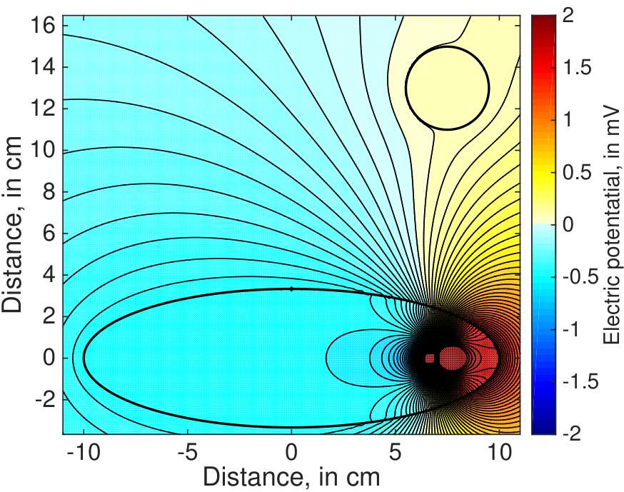
Using layer potential representations for the solutions of the systems (2.15-2.19) and (2.20-2.22), we have developed a MATLAB script for their numerical approximations¹¹ 1 This script is now part of the package SIES (Shape Identification in Electro-Sensing), which can be found at https://github.com/ens2013/SIES/, using boundary element methods like in Assad’s thesis [10]. In Figure 3, we have plotted the solutions $u$ and $U$ when $d=2$, the body $\Omega$ is an ellipse, the object $D$ is a disk, and the source $f$ is a dipole.

The dipolar approximation states that if $D$ is small enough, the difference $u-U$ can be expressed as the electric potential coming from an electric dipole centered in $D$. In this subsection we only present this result numerically, in order to make things more intuitive. For a complete proof of the formula in this context, see [1]; for a more detailed review of the dipolar approximation in general, see the book [5].

Let us get back to the example in Section 2.3. In Figure 4, we have plotted the difference $u-U$. Qualitatively, we can see that this electric potential looks like the one emitted by an electric dipole coming from $D$.

Quantitatively, we have shown in [1] that, if $D$ is small enough and sufficiently away from $\Omega$, then the fish feels a distorsion that is similar to the one produced by a dipole $\itbf{p}_{D}$. More precisely, we have

where $\itbf{z}$ is the center of mass of $D$ and $G$ is the Green function for the Laplacian in $\mathbb{R}^{d}$ (for instance $G(\itbf{x})=\log(|\itbf{x}|)/(2\pi)$ in dimension $d=2$ or $G(\itbf{x})=-1/(4\pi|\itbf{x}|)$ in dimension $d=3$). The vector $\itbf{p}_{D}$ is called the equivalent dipole, and it is given by

where ${\bf M}(k_{D}(\omega),D)$ is a $d\times d$ complex-valued matrix that depends only on the shape $D$ of the object and its complex conductivity $k_{D}(\omega)$, called the first-order polarization tensor [5]. This matrix maps the illuminating electric field $\nabla U(\itbf{z})$ to the equivalent dipole $\itbf{p}_{D}$. When the conductivity $k_{D}(\omega)$ is real, in other words when $\Im(k_{D}(\omega))=0$ and thus $\omega$ does not play any role anymore, one can find an ellipse or ellipsoid $\mathcal{E}$ such that

This means that the equivalent dipole would always be the same as the equivalent dipole of this ellipse or ellipsoid $\mathcal{E}$. This latter is then called the equivalent ellipse [5]. Note, however, that when $k_{D}(\omega)$ is frequency-dependent, the information that can be extracted is much richer. For single-frequency data, it is only possible to identify a few characteristics of the object. When multi-frequency data are available, it is possible to get a lot of information about the object from the frequency dependence of the observed first-order polarization tensors. The need for multi-frequency data that we exhibit is in agreement with the complex emission patterns (pulse and wave) by fish.

In this subsection, we show that the multi-frequency aspect of the measurements are sufficient to localize an object with precision. For the sake of simplicity we focus our attention on the example that gave Figures 3-4 in dimension $d=2$. Indeed, the particular case of $D$ being a disk is easier since we have [5]

where $|D|$ denotes the volume of $D$ and ${\bf I}_{2}$ is the identity matrix.²² 2 In $\mathbb{R}^{3}$, we have a similar formula, i.e. ${\bf M}(k_{D}(\omega),D)$ is proportional to identity [5, p. 83]. Hence, equation (3.1) becomes

which is equivalent to Lissman-Machin [32] or Rasnow [39] formulas, showing that (3.1) is a generalization of these latters. Hence, from (3.5) we can easily extract $\nabla U(\itbf{z})\cdot\nabla G(\itbf{x}-\itbf{z})$. The reason why we can recover the location $\itbf{z}$ of $D$ is that the function $\itbf{z}\mapsto\nabla U(\itbf{z})\cdot\nabla G(\itbf{x}-\itbf{z})$ is one-to-one. Therefore, it is possible to build an imaging functional from the measured data, i.e. a function $\itbf{z}_{s}\mapsto\mathcal{I}(\itbf{z}_{s})$ that has a strong peak at $\itbf{z}_{s}=\itbf{z}$ (see Figure 5).

Once the object $D$ is located (i.e. we know $\itbf{z}$), we would like to extract ${\bf M}(k_{D}(\omega),D)$ from the measurements. Indeed, we know that this polarization tensor contains all the necessary information about the shape of $D$ [7]. More precisely, the function $\omega\mapsto{\bf M}(k_{D}(\omega),D)$ uniquely determines $D$ in some class of domains. However, it is not straighfoward to determine $D$ from ${\bf M}(k_{D}(\omega),D)$. In other words, the shape recognition problem has been reduced to a simpler, however still difficult, inverse problem: determine the shape of the object from the observed first-order polarization tensors.

To solve this inverse problem we got inspired by the behavioral studies (for example [48]) described in the introduction. Indeed, instead of trying to compute a shape from the measurements, we wanted to use classification and machine learning techniques. For example, let us suppose that the fish has already encountered several shapes $D_{l}$, $p=1,\ldots,L$ (such as the shapes plotted in Figure 6), and that it knows all the polarization tensors ${\bf M}(k_{D_{l}}(\omega_{j}),D_{l})$, where $\omega_{j}$ are the different frequencies emitted by the electric organ.

It is not possible to extract ${\bf M}(k_{D}(\omega),D)$ from one single measure of $\frac{\partial u}{\partial\nu}-\frac{\partial U}{\partial\nu}$; instead, we use the fact that the fish actively swim around their prey when hunting, leading to particular swimming patterns called probing motor acts [44]. Extracting ${\bf M}(k_{D}(\omega_{j}),D)$ from (3.1) measured for several fish’s positions is then a simple linear system [3]. Hence, $D$ can be identified as

In Figure 7, one can see the performance of this technique in terms of robustness against measurement noise. Note that the number $64$ of electrodes is not very large in the numerical simulations, but $10$ frequencies and $20$ different positions of the fish around the object are exploited: the different positions allow for good extraction of the polarization tensors, and the different frequencies allow for good classification of the object given the estimated polarization tensors. That is how robustness is achieved, and this remark may be of interest for the design of EIT devices.

The authors would like to thank the reviewers for their very constructive remarks.

References

- [1] Habib Ammari, Thomas Boulier, and Josselin Garnier. Modeling active electrolocation in weakly electric fish. SIAM Journal on Imaging Sciences, 6(1):285–321, 2013.
- [2] Habib Ammari, Thomas Boulier, Josselin Garnier, Hyeonbae Kang, and Han Wang. Tracking of a mobile target using generalized polarization tensors. SIAM Journal on Imaging Sciences, 6(3):1477–1498, 2013.
- [3] Habib Ammari, Thomas Boulier, Josselin Garnier, and Han Wang. Shape recognition and classification in electro-sensing. Proceedings of the National Academy of Sciences, 111(32):11652–11657, 2014.
- [4] Habib Ammari and Hyeonbae Kang. Reconstruction of small inhomogeneities from boundary measurements, volume 1846. Springer Science & Business Media, 2004.
- [5] Habib Ammari and Hyeonbae Kang. Polarization and moment tensors: with applications to inverse problems and effective medium theory, volume 162. Springer Science & Business Media, 2007.
- [6] Habib Ammari, Stéphane Mallat, Irène Waldspurger, and Han Wang. Wavelet methods for shape perception in electro-sensing. In Imaging, Multi-scale and High Contrast Partial Differential Equations. American Mathematical Society, 2016.
- [7] Habib Ammari, Mihai Putinar, Matias Ruiz, Sanghyeon Yu, and Hai Zhang. Shape reconstruction of nanoparticles from their associated plasmonic resonances. arXiv preprint arXiv:1602.05268, 2016.
- [8] Habib Ammari, Minh Phuong Tran, and Han Wang. Shape identification and classification in echolocation. SIAM Journal on Imaging Sciences, 7(3):1883–1905, 2014.
- [9] Habib Ammari and Han Wang. Time-domain multiscale shape identification in electro-sensing. In Habib Ammari, Yves Capdeboscq, Hyeonbae Kang, and Sim Imbo, editors, Imaging, Multi-scale and High Contrast Partial Differential Equations, chapter 2, pages 23–45. AMS (eBook Collections), 2016.
- [10] Christopher Assad. Electric field maps and boundary element simulations of electrolocation in weakly electric fish. PhD thesis, California Institute of Technology, 1997.
- [11] David Babineau, John E Lewis, and André Longtin. Spatial acuity and prey detection in weakly electric fish. PLoS Comput Biol, 3(3):e38, 2007.
- [12] David Babineau, André Longtin, and John E Lewis. Modeling the electric field of weakly electric fish. Journal of experimental biology, 209(18):3636–3651, 2006.
- [13] M Bacher. A new method for the simulation of electric fields, generated by electric fish, and their distorsions by objects. Biological cybernetics, 47(1):51–58, 1983.
- [14] Yang Bai, James B. Snyder, Michael Peshkin, and Malcolm A. MacIver. Finding and identifying simple objects underwater with active electrosense. The International Journal of Robotics Research, 34(10):1255–1277, 2015.
- [15] Liliana Borcea. Electrical impedance tomography. Inverse Problems, 18, 2002.
- [16] Frédéric Boyer, Pol Bernard Gossiaux, Brahim Jawad, Vincent Lebastard, and Mathieu Porez. Model for a sensor inspired by electric fish. IEEE Transactions on Robotics, 28(2):492–505, 2012.
- [17] Frederic Boyer, Vincent Lebastard, Christine Chevallereau, Stefano Mintchev, and Cesare Stefanini. Underwater navigation based on passive electric sense: New perspectives for underwater docking. The International Journal of Robotics Research, 34(9):1228–1250, 2015.
- [18] Frédéric Boyer, Vincent Lebastard, Christine Chevallereau, and Noël Servagent. Underwater reflex navigation in confined environment based on electric sense. IEEE transactions on robotics, 29(4):945–956, 2013.
- [19] Brian H. Brown. Electrical impedance tomography (eit): a review. J. Med. Eng. Technol., 27(3):97–108, 2003.
- [20] Ruben Budelli and Angel A Caputi. The electric image in weakly electric fish: perception of objects of complex impedance. Journal of Experimental Biology, 203(3):481–492, 2000.
- [21] Alberto P. Calderón. On an inverse boundary value problem. In Seminar on Numerical Analysis and its Applications to Continuum Physics, pages 65–73. Soc. Brasil. Mat. (Rio de Janeiro), 1980.
- [22] Margaret Cheney, David Isaacson, and Jonathan C Newell. Electrical impedance tomography. SIAM review, 41(1):85–101, 1999.
- [23] KD Dunlap, P Thomas, and HH Zakon. Diversity of sexual dimorphism in electrocommunication signals and its androgen regulation in a genus of electric fish, apteronotus. Journal of Comparative Physiology A, 183(1):77–86, 1998.
- [24] DH Evans and JB Claiborne. The physiology of fishes. Boca Raton, FL, CRC Taylor & Francis, 2006.
- [25] Stanley Finger and Marco Piccolino. The shocking history of electric fishes: from ancient epochs to the birth of modern neurophysiology. Oxford University Press, 2011.
- [26] Walter Heiligenberg. Theoretical and experimental approaches to spatial aspects of electrolocation. Journal of comparative physiology, 103(3):247–272, 1975.
- [27] N Hoshimiya, K Shogen, T Matsuo, and S Chichibu. Theapteronotus eod field: Waveform and eod field simulation. Journal of Comparative Physiology A: Neuroethology, Sensory, Neural, and Behavioral Physiology, 135(4):283–290, 1980.
- [28] Ludger Klinkenbusch, Wolfgang Mathis, Thorsten Steinmetz, Stefan Kurz, and Markus Clemens. Domains of validity of quasistatic and quasistationary field approximations. COMPEL-The international journal for computation and mathematics in electrical and electronic engineering, 30(4):1237–1247, 2011.
- [29] Sylvain Lanneau, Vincent Lebastard, et al. Object shape recognition using electric sense and ellipsoid’s polarization tensor. In 2016 IEEE International Conference on Robotics and Automation (ICRA), pages 4692–4699. IEEE, 2016.
- [30] Vincent Lebastard, Christine Chevallereau, Alexis Girin, Noël Servagent, Pol-Bernard Gossiaux, and Frédéric Boyer. Environment reconstruction and navigation with electric sense based on a kalman filter. The International Journal of Robotics Research, 32(2):172–188, 2013.
- [31] John E Lewis and Leonard Maler. Neuronal population codes and the perception of object distance in weakly electric fish. The Journal of Neuroscience, 21(8):2842–2850, 2001.
- [32] HW Lissmann and KE Machin. The mechanism of object location in gymnarchus niloticus and similar fish. Journal of Experimental Biology, 35(2):451–486, 1958.
- [33] Malcolm A Maciver. The computational neuroethology of weakly electric fish: body modeling, motion analysis, and sensory signal estimation. PhD thesis, University of Illinois at Urbana-Champaign, 2001.
- [34] Malcolm A. MacIver, Ebraheem Fontaine, and Joel W. Burdick. Designing future underwater vehicles: principles and mechanisms of the weakly electric fish. IEEE Journal of Oceanic Engineering, 29(3):651–659, 2004.
- [35] Malcolm A Maciver, Noura M Sharabash, and Mark E Nelson. Prey-capture behavior in gymnotid electric fish: motion analysis and effects of water conductivity. Journal of experimental biology, 204(3):543–557, 2001.
- [36] Adriana Migliaro, Angel A Caputi, and Ruben Budelli. Theoretical analysis of pre-receptor image conditioning in weakly electric fish. PLoS Comput Biol, 1(2):e16, 2005.
- [37] Peter Moller. Electric fishes: history and behavior, volume 17. Chapman & Hall London, 1995.
- [38] Mark E Nelson and Malcolm A MacIver. Sensory acquisition in active sensing systems. Journal of Comparative Physiology A, 192(6):573–586, 2006.
- [39] Brian Rasnow. The effects of simple objects on the electric field of apteronotus. Journal of Comparative Physiology A, 178(3):397–411, 1996.
- [40] Brian Rasnow, Christopher Assad, Mark E Nelson, and James M Bower. Simulation and measurement of the electric fields generated by weakly electric fish. In NIPS, pages 436–443, 1988.
- [41] Gary Rose and Walter Heiligenberg. Temporal hyperacuity in the electric sense of fish. Nature, 1985.
- [42] H Scheich, Th H Bullock, and RH Hamstra. Coding properties of two classes of afferent nerve fibers: high-frequency electroreceptors in the electric fish, eigenmannia. Journal of Neurophysiology, 36(1):39–60, 1973.
- [43] James R Solberg, Kevin M Lynch, and Malcolm A MacIver. Active electrolocation for underwater target localization. The International Journal of Robotics Research, 27(5):529–548, 2008.
- [44] MJ Toerring and P Belbenoit. Motor programmes and electroreception in mormyrid fish. Behavioral Ecology and Sociobiology, 4(4):369–379, 1979.
- [45] Gunther Uhlmann. Calderon’s problem and electrical impedance tomography. Inverse Problems, 25:123011, 2009.
- [46] Gerhard Von der Emde. Active electrolocation of objects in weakly electric fish. Journal of experimental biology, 202(10):1205–1215, 1999.
- [47] Gerhard von der Emde and Steffen Fetz. Distance, shape and more: recognition of object features during active electrolocation in a weakly electric fish. Journal of Experimental Biology, 210(17):3082–3095, 2007.
- [48] Gerhard Von Der Emde, Stephan Schwarz, Leonel Gomez, Ruben Budelli, and Kirsty Grant. Electric fish measure distance in the dark. Nature, 395(6705):890–894, 1998.
- [49] Harold Zakon. The electroreceptive periphery. Electroreception. Wiley, New York, pages 103–156, 1986.