A Landauer-Büttiker approach for hyperfine mediated electronic transport in the integer quantum Hall regime.

In order to describe the electron-nuclear hyperfine interaction, we start with the Fermi contact hyperfine interaction Hamiltonian for the case with non-varying electronic density of states in space, given by [2]

$$\hat{H}_{HF}(\textbf{r}_{n})=\sum_{n}A_{eff}\psi^{*}(\textbf{r}_{n})\psi(\bf{r}_{n})a_{0}^{3}\left[\hat{S}_{z}\otimes\hat{I}_{z}^{n}+\left\{\frac{\hat{I}_{+}^{n}\otimes\hat{S}_{-}+\hat{S}_{+}\otimes\hat{I}_{-}^{n}}{2}\right\}\right],$$

(1)

where $\psi(\bf{r}_{n})$ represents the electron wavefunction at the point $\bf{r}_{n}$, with $\psi^{*}(\bf{r}_{n})\psi(\bf{r}_{n})$ representing the effective electron density per unit volume at the point $\bf{r}_{n}$, $A_{eff}$ is the effective hyperfine coupling constant, $\hat{S}_{z},\hat{I}^{n}_{z}$ are the operators representing the $z$ component of the electronic spin and the nuclear spin respectively, with $a_{0}^{3}$ representing a unit cell volume. The operator $`\otimes^{\prime}$ represents the tensor product between the electron spin and the nuclear spin spaces. The operators, $\hat{S}_{+(-)}$ and $\hat{I}_{+(-)}^{n}$ are respectively the corresponding spin raising (lowering) operators for the electron and the nuclear spins respectively. The above equation assumes $\psi_{\uparrow}(\textbf{r}_{n})=\psi_{\downarrow}(\textbf{r}_{n})=\psi(\textbf{r}_{n})$, where ‘$\uparrow$’ and ‘$\downarrow$’ represents the eigen states in the electron spin-space. In the quantum Hall regime, however, the eigen states are localized in space along the transverse direction. In this case, $\psi_{\uparrow}(\textbf{r}_{n})\neq\psi_{\downarrow}(\textbf{r}_{n})$ and thus the Hamiltonian should be recast in the form [28, 29, 30]:

$$\displaystyle\hat{H}_{HF}(\textbf{r}_{n})=A_{eff}a_{0}^{3}\bf\sum_{\ket{\phi,\beta}\bra{\varphi,\alpha}}\bra{\phi,\beta}\left[\hat{S}_{z}\otimes\hat{I}_{z}^{n}+\left\{\frac{\hat{I}_{+}^{n}\otimes\hat{S}_{-}+\hat{S}_{+}\otimes\hat{I}_{-}^{n}}{2}\right\}\right]\ket{\varphi,\alpha}\times\sum_{n}\Big\{\bra{\psi^{}_{\beta}}\ket{\textbf{r}_n}\ket{\phi,\beta}\bra{\varphi,\alpha}\bra{\textbf{r}_n}\ket{\psi_{\alpha}}\Big\},$$

where $\ket{\phi, \beta}=\ket{\phi}\otimes\ket{\beta}$ and $\ket{\varphi, \alpha}=\ket{\varphi}\otimes\ket{\alpha}$ with $\ket{\alpha}$ and $\ket{\beta}$ belonging to the electron spin-space and $\ket{\phi}$ and $\ket{\varphi}$ belonging to the nuclear-spin space in the presence of a magnetic field pointing along the $z-$ direction. When the coupling constant $A_{eff}$ is small, the effect of the two terms in (1) can be separated. The first term results in an effective magnetic field and the second term within the curly brackets represents the electron-nuclear spin flip-flop processes. The first term in (1), which also corresponds to $\ket{\alpha}=\ket{\beta}$ and $\ket{\phi}=\ket{\varphi}$ in () introduces an additional shift in the electronic energy levels as well as between states of different nuclear spins. The electronic energy difference $\Delta$ between the up-spin channel electrons and the down-spin channel electrons is given by [31]

$$\Delta=g_{el}\mu_{B}B_{app}+A_{eff}<I_{z}>,$$

(3)

where $g_{el}$, $\mu_{B}$ and $B_{app}$ are the effective Lande $g$-factor of the electron in GaAs, the Bohr magneton and the applied magnetic field respectively. The above expression is obtained by assuming an isotropic nuclear spin distribution. Similarly, the energy difference $\epsilon$ between the adjacent nuclear spin states differing by a magnetic quantum number of $\Delta s=\pm 1$ is given by

$$\epsilon=g_{nuc}\mu_{B}^{nuc}B_{app}+A^{\prime\prime}<S_{z}>,$$

(4)

where $g_{nuc}$ is the effective Lande $g$-factor of the nuclide in consideration and $\mu_{B}^{nuc}$ is the nuclear Bohr magneton. The effective coupling constant $A^{\prime\prime}=A_{eff}a_{0}^{3}n_{el}$ [32, 31, 2], where $n_{el}$ is the electronic carrier density. The magnetic quantum number for the GaAs nuclei varies from $-3/2$ to $+3/2$ in steps of $\Delta s=+1$. In standard literature, the second terms in (3) and (4) represent the Overhauser shift and the Knight shift respectively. However, for practical purposes, $g_{nuc}<<g_{el}$ and $A^{\prime\prime}<<A_{eff}$ and hence $\epsilon$ may be neglected with respect to $\Delta$ and the nuclear spin flips may be considered elastic.
The electron-nuclear spin flip-flop processes are described by the second term in the Hamiltonian in (1), which also corresponds to $\ket{\alpha}\neq\ket{\beta}$ and $\ket{\phi}\neq\ket{\varphi}$ in () and the scattering rates are evaluated via the Fermi’s golden rule [33, 34], typically related to the densities of the initial and the final states. In this case, the electronic wavefunction distribution $\psi_{\alpha}(\bf{r}_{n})$ and $\psi_{\beta}(\bf{r}_{n})$ overlaps with the nuclear wavefunction on each site $\bf{r_{n}}$ differently, and this effect is accounted for via the overlap terms $\psi^{*}_{\beta}(\bf{r}_{n})\psi_{\alpha}(\bf{r}_{n})$ for up to down or down to up electronic spin transitions. The procedure for a self-consistent description of electronic transport coupled to hyperfine spin dynamics then entails the time-dependent simulation of the nuclear spin dynamics, with the electronic transport processes in steady state. This is because the nuclear spin dynamics are typically slow due to slow relaxation rates, slow diffusion rates as well as longer flip-flop times in comparison with the electronic transport velocities. The nuclear spin dynamics at each point $\bf{r}_{n}$ are dictated via the electron-nuclear hyperfine flip rates calculated from the Fermi’s golden rule [33] given by:

	$\displaystyle\Gamma_{\uparrow\downarrow}(\textbf{r}_{n})=\frac{2\pi}{\hbar}\mid A_{eff}\mid^{2}\int dEn_{\uparrow}(\textbf{r}_{n},E)p_{\downarrow}(\textbf{r}_{n},E)$
	$\displaystyle\Gamma_{\downarrow\uparrow}(\textbf{r}_{n})=\frac{2\pi}{\hbar}\mid A_{eff}\mid^{2}\int dEn_{\downarrow}(\textbf{r}_{n},E)p_{\uparrow}(\textbf{r}_{n},E),$
			(5)

where $\Gamma_{\downarrow\uparrow}(\textbf{r}_{n})$ ($\Gamma_{\uparrow\downarrow}(\textbf{r}_{n})$) represents the up to down (down to up) nuclear spin transition rate at the nuclear co-ordinate $\bf{r}_{n}$ between magnetic quantum numbers that differ by $+1$ ($-1$) in the nuclear spin space due to flip-flop transitions of electrons at energy $E$. The quantities $n_{\uparrow}(\textbf{r}_{n},E)$ and $n_{\downarrow}(\textbf{r}_{n},E)$ ($p_{\uparrow}(\textbf{r}_{n},E)$ and $p_{\downarrow}(\textbf{r}_{n},E)$) denote the densities of filled (vacant) states per unit energy per unit area at the point $\textbf{r}_{n}$. \colorblack The up to down (down to up) electronic spin transition rate based on (5) depends not only on the the availability of electrons in the up (down) spin density of states $D_{\uparrow(\downarrow)}(\textbf{r}_{n},E)$ and the vacancy in the down (up) spin density of states $D_{\downarrow(\uparrow)}(\textbf{r}_{n},E)$, but also on the spatial overlap of the corresponding density of states. The total rate of electron-nuclear spin flip-flop now depends on the integral of $\Gamma_{\downarrow\uparrow}(\textbf{r}_{n})$ ($\Gamma_{\uparrow\downarrow}(\textbf{r}_{n})$) over the spatial co-ordinates.

	$\displaystyle\Gamma_{\uparrow\downarrow}=\frac{2\pi}{\hbar}\mid A_{eff}\mid^{2}\int\int d^{3}\textbf{r}_{n}dEn_{\uparrow}(\textbf{r}_{n},E)p_{\downarrow}(\textbf{r}_{n},E)$
	$\displaystyle\Gamma_{\downarrow\uparrow}=\frac{2\pi}{\hbar}\mid A_{eff}\mid^{2}\int\int d^{3}\textbf{r}_{n}dEn_{\downarrow}(\textbf{r}_{n},E)p_{\uparrow}(\textbf{r}_{n},E)$
			(6)

The spatial dynamics of the nuclear spins can be described by the following master equation:

	$\displaystyle\frac{d\left[F(\textbf{r}_{n})\right]}{dt}=\left[\Gamma(\textbf{r}_{n})\right]\left[F(\textbf{r}_{n})\right]-\frac{[F(\textbf{r}_{n})-F^{0}]}{\tau_{I}}$
	$\displaystyle+D_{n}{\nabla}^{2}[F(\textbf{r}_{n})],$
			(7)

where $\left[{F(\bf{r}_{n})}\right]$ is the probability column vector representing the probability of occupancy of the nuclear spin levels, and $\tau_{I}$ is a phenomenological nuclear spin relaxation time, which is typically a very slow process. The matrix $\Gamma(\textbf{r}_{n})$ takes into account the transition between the individual nuclear spin levels. The vector $\left[F^{0}\right]$ denotes the probability of occupation of the nuclear spin levels in equilibrium. The above equation also includes nuclear spin diffusion described by the last term, where $D_{n}$ is the phenomenological diffusion constant. In this paper, we neglect the exact spatial distribution of nuclear spins due to diffusion and approximate the effects of nuclear spin diffusion by incorporating a larger number of nuclei. The equation governing the dynamics of the nuclear spins is then given by:

$$\frac{d\left[F\right]}{dt}=\left[\Gamma\right]\left[F\right]-\frac{\left[F-F^{0}\right]}{\tau_{I}}.$$

(8)

The transition probability matrix $[\Gamma]$ may be specifically cast for the spin-$3/2$ case in the current study in terms of the spin-flip rates defined in (6) as:

	$\displaystyle\left[\Gamma\right]=\begin{bmatrix}-\Gamma_{\downarrow\uparrow}&\Gamma_{\uparrow\downarrow}&0&0\\ \Gamma_{\downarrow\uparrow}&-\left(\Gamma_{\downarrow\uparrow}+\Gamma_{\uparrow\downarrow}\right)&\Gamma_{\uparrow\downarrow}&0\\ 0&\Gamma_{\downarrow\uparrow}&-\left(\Gamma_{\downarrow\uparrow}+\Gamma_{\uparrow\downarrow}\right)&\Gamma_{\uparrow\downarrow}\\ 0&0&\Gamma_{\downarrow\uparrow}&-\Gamma_{\uparrow\downarrow}\end{bmatrix},$
			(9)

where $\Gamma_{\uparrow\downarrow}$ and $\Gamma_{\downarrow\uparrow}$ are defined in (6). An additional constraint used to solve (8) using (9) is that of the normalization of the nuclear state probabilities, i.e., $\sum_{s}F_{s}=1$, where $F_{s}$ is the occupation probability of the nuclear density of states with spin $s$.
The temporal evolution of the average electronic polarization $<S_{z}>$ and the average nuclear polarization $<I_{z}>$ at the QPC are calculated self-consistently by solving (8) and (3) via the relations:

	$$\displaystyle<S_{z}>=\frac{1}{2}\frac{n_{\uparrow}-n_{\downarrow}}{n_{\uparrow}+n_{\downarrow}}$$
	$$\displaystyle F_{I}=<I_{z}>=\sum_{s}sF_{s}=\left[s\right]\left[F\right],$$		(10)

where $F_{s}$ are obtained by solving the master equations. The matrix $[s]=\left[\frac{3}{2}~~\frac{1}{2}~~-\frac{1}{2}~~-\frac{3}{2}\right]$ comprises the row vector of the spin magnetic quantum numbers of the GaAs nuclei. The procedure for transport calculations follows solving (3), (8), and (10) sequentially in a self-consistent loop with the electronic transport to be described now.

While the dynamics of the nuclear spins simply follow the master equation (8) described above, a description of electronic transport involves transport currents due to the source and drain reservoirs held at electrochemical potentials $\mu_{S}$ and $\mu_{D}$ respectively. From a Landauer-Büttikker perspective, a consistent description of transport currents in our case demands the use of both a) direct transmission and b) spin-flip transmission. The need to include spin flip transmission follows from the interaction between the edge channels of different spins that gives rise to nuclear polarization which in close proximity of the QPC region determines the electronic transport. Near the QPC, the forward propagating edge channels and the backward propagating edge channels come in close proximity and hence spin-flip scattering can occur to the forward propagating as well as to the backward propagating edge channels [3].
The Landauer direct transmission $T_{\uparrow(\downarrow)}(E)$ denotes the tunneling probability of the up (down)-spin electrons through the QPC. We model the spin-split edge states in the device by a continuum of density of states as in a ballistic $1-D$ conductor [35, 36, 37, 38] with the region of the QPC being represented by a Gaussian potential barrier, as shown in Fig. 2 (a) and (b) along with the model used for simulation of electronic transport shown in Fig. 2 (c). The direct transmission coefficients $T_{\uparrow}(E)$ and $T_{\downarrow}(E)$ are then calculated using the non-equilibrium Green’s function (NEGF) method applied to the barrier described above using a $1-D$ atomistic tight-binding Hamiltonian [39, 40]. The pertinent details of the approach used here have been briefly discussed in Appendix B. In our scheme, we only consider the number of transmitted modes and the filling factor at the QPC for the electronic transport which is related to the geometry of the set up that is ascertained apriori. Near the vicinity of $\nu_{QPC}=1$ at the QPC, the down-spin edge channel at the QPC is almost empty in the energy range between $\mu_{S}$ and $\mu_{D}$, resulting in a considerable simplification of the transport equations.
We begin with the case where the filling factor $\nu_{QPC}<1$, i.e., $G<\frac{e^{2}}{h}$, where only the up-spin edge channel originating from the source contact contributes to the total current terminating in the drain contact. The electrons in the forward propagating up-spin edge channel originating from the source contact can tunnel through the QPC to the up-spin edge channel terminating in the drain contact with a probability $T_{\uparrow}(E)$ while the forward propagating down-spin edge channel originating in the source contact is completely disconnected from the forward propagating down-spin edge channel terminating in the drain contact, as depicted in Fig. 2(a) and (b) respectively.
A few up-spin electrons at the QPC in the forward propagating edge channel terminating in the drain contact can however scatter to the forward propagating down-spin edge channel terminating in the drain contact with a spin-flip process as shown in Fig. 3 (a). This gives rise to the spin-flip scattering current $I^{sf}_{\uparrow\downarrow(\downarrow\uparrow)}$, where the superscript ‘$sf$’ denotes the flow of current due to spin-flip scattering at the QPC and the subscript ${}^{\prime}\uparrow\downarrow(\downarrow\uparrow)^{\prime}$ denotes the current flow from the up (down)-spin to down (up)-spin edge channel via electronic spin-flips. Assuming that the direct transmission coefficients ($T_{\uparrow}$ and $T_{\downarrow}$) depend on the nuclear polarization only via the Overhauser field (3), for a system with four nuclear spin levels, the spin-flip transmission coefficient at the QPC from the forward propagating up-spin channel terminating in the drain contact to the forward propagating down-spin channel terminating in the drain contact is given by (details given in Appendix A):

$$T_{\uparrow\downarrow}^{sff}(E)=T_{\uparrow}(E)T_{\uparrow\downarrow}^{f}\Big\{1-F_{+\frac{3}{2}}\Big\}.$$

Note that $T_{\uparrow\downarrow}^{f}$ depends on the spatial overlap of the density of states of the up-spin and down-spin edge channel at the QPC between the energy range $\mu_{S}$ and $\mu_{D}$ (details given in Appendix A, Eq. 32 and 37). We approximate $T_{\uparrow\downarrow}^{f}$ as a constant. Therefore, the down-spin current recorded just outside the QPC relies entirely on such spin-flip processes and hence is simply the spin-flip current $I^{sf}_{\uparrow\downarrow}$ while the up-spin current in the edge channel just outside the QPC is reduced by $I^{sf}_{\uparrow\downarrow}$. Based on the above discussions, the up and down spin channel currents are given by

$$I=\int dE\left(I_{\uparrow}(E)+I_{\downarrow}(E)\right)$$

$$=\frac{q}{h}\int dE\Big\{[T_{\uparrow}(E)-T^{sff}_{\uparrow\downarrow}(E)]+T^{sff}_{\uparrow\downarrow}(E)\Big\}\\ \times\Big\{f_{S}(E)-f_{D}(E)\Big\}.$$

(11)

The subscripts ${}^{\prime}S^{\prime}$ and ${}^{\prime}D^{\prime}$ the source and drain contacts respectively, with $f_{S(D)}(E)$ denoting the Fermi-Dirac distribution in the source (drain) contact held in quasi-equilibrium at $\mu_{S(D)}$. The parameter $T_{\uparrow\downarrow}^{sff}(E)$ takes into account the spin-flip scattering of electrons at and around the QPC from the forward propagating up-spin edge channel terminating in the drain contact to the forward propagating down-spin channel terminating in the drain contact, with the superscript ${}^{\prime}sff^{\prime}$ denoting spin-flip scattering to a forward propagating channel. It must be noted that the edge channels in the quantum Hall arrangement are uni-directional and hence the expressions for the current in (11) depend on the factors $f_{S}(E)$ and $f_{D}(E)$ only and not on the factors $f_{S}(E)\{1-f_{D}(E)\}$ and $f_{D}(E)\{1-f_{S}(E)\}$ as expected in a typical Landauer type scattering treatment.
Turning our attention to the case when the filling factor $\nu_{QPC}>1$, i.e., $G>\frac{e^{2}}{h}$, the down-spin electrons in the edge channel originating in the source contact are partially transmitted through the QPC to the down-spin edge channel terminating in the drain contact, as depicted in Fig. 3(b). In this case, the spin-flip scattering at and around the QPC can occur from the forward propagating up-spin channel terminating in the drain contact to the forward propagating down-spin channel terminating in the drain contact as well as from the forward propagating down-spin channel terminating in the drain contact to the backward propagating up-spin channel originating from the drain contact. Again, assuming that the direct transmission coefficients $T_{\uparrow}$ and $T_{\downarrow}$ depend on the nuclear polarization only via the Overhauser field (3), the spin-flip currents in this case are given by (details in Appendix A)

	$\displaystyle I_{\uparrow\downarrow}^{sf}$	$\displaystyle\approx\frac{q}{h}\int dET_{\uparrow\downarrow}^{sff}(E)\Big(f_{S}(E)-f_{D}(E)\Big)$
	$\displaystyle I_{\downarrow\uparrow}^{sf}$	$\displaystyle\approx\frac{q}{h}\int dET_{\downarrow\uparrow}^{sfb}(E)\Big(f_{S}(E)-f_{D}(E)\Big),$

where superscript ${}^{\prime}sfb^{\prime}$ denote spin-flip scattering to a backward propagating edge channel while the superscript ${}^{\prime}sff^{\prime}$ has the same meaning as described previously. The spin-flip current $I_{\uparrow\downarrow}^{sf}$ flows from the forward propagating up-spin channel terminating in the drain contact to the forward propagating down-spin edge channel terminating in the drain contact while the spin-flip current $I_{\downarrow\uparrow}^{sf}$ flows from the forward propagating down-spin edge channel terminating in the drain contact to the backward propagating up-spin channel originating in the drain contact. Hence, $I_{\downarrow\uparrow}^{sf}$ causes a change in the total output current since the spin-flip scattering occurs to a backward propagating edge channel. It however does play a role in the nuclei polarization near the QPC. The current in the up-spin and down-spin channel terminating in the drain contact just outside the QPC is then given by:

$$I_{\uparrow}=\int\frac{q}{h}\{T_{\uparrow}(E)-T_{\uparrow\downarrow}^{sff}(E)\}\{f_{S}(E)-f_{D}(E)\}dE$$

$$=\int\frac{q}{h}\{T_{\uparrow}(E)-T_{\uparrow}(E)T_{\uparrow\downarrow}^{f}(1-F_{\frac{3}{2}})\}\\ \times\{f_{S}(E)-f_{D}(E)\}dE$$

(12)

$$I_{\downarrow}=\int\frac{q}{h}\{T_{\downarrow}(E)+T_{\uparrow\downarrow}^{sff}(E)-T_{\downarrow\uparrow}^{sfb}(E)\}\{f_{S}(E)-f_{D}(E)\}dE$$

$$=\int\frac{q}{h}\{T_{\downarrow}(E)+T_{\uparrow}(E)T_{\uparrow\downarrow}^{f}(1-F_{\frac{3}{2}})-T_{\downarrow}(E)T_{\downarrow\uparrow}^{b}(1-F_{-\frac{3}{2}})\}\\ \times\{f_{S}(E)-f_{D}(E)\}dE$$

(13)

From the above discussion, the generalized equations for the up-spin, down-spin and spin-flip currents through the QPC are given by:

	$\displaystyle I_{\uparrow}$	$\displaystyle=\frac{q}{h}\int\Big\{\underbrace{T_{\uparrow}(E)}_{\frac{Direct}{Transmission}}+~~~\underbrace{T^{sff}_{\downarrow\uparrow}(E)-T^{sff}_{\uparrow\downarrow}(E)}_{\frac{spin~flip}{forward~transmission}}~~~~~-\underbrace{T^{sfb}_{\uparrow\downarrow}(E)}_{\frac{spin~flip}{backward~transmission}}\Big\}\times\{f_{S}(E)-f_{D}(E)\}dE$
		$\displaystyle=\frac{q}{h}\int\Big\{{T_{\uparrow}(E)}+{T_{\downarrow\uparrow}^{f}T_{\downarrow}(E)\{1-F_{-\frac{3}{2}}\}-T_{\uparrow\downarrow}^{f}T_{\uparrow}(E)\{1-F_{\frac{3}{2}}\}-T_{\uparrow\downarrow}^{b}T_{\uparrow}(E)\{1-F_{\frac{3}{2}}\}}\Big\}\times\{f_{S}(E)-f_{D}(E)\}dE$
	$\displaystyle I_{\downarrow}$	$\displaystyle=\frac{q}{h}\int\Big\{\underbrace{T_{\downarrow}(E)}_{\frac{Direct}{Transmission}}+~~~\underbrace{T^{sff}_{\uparrow\downarrow}(E)-T^{sff}_{\downarrow\uparrow}(E)}_{\frac{spin~flip}{forward~transmission}}~~~~-\underbrace{T^{sfb}_{\downarrow\uparrow}(E)}_{\frac{spin~flip}{backward~transmission}}\Big\}\times\{f_{S}(E)-f_{D}(E)\}dE$
		$\displaystyle=\frac{q}{h}\int\Big\{{T_{\downarrow}(E)}+{T_{\uparrow\downarrow}^{f}T_{\uparrow}(E)\{1-F_{\frac{3}{2}}\}-T_{\downarrow\uparrow}^{f}T_{\downarrow}(E)\{1-F_{-\frac{3}{2}}\}-T_{\downarrow\uparrow}^{b}T_{\downarrow}(E)\{1-F_{-\frac{3}{2}}\}}\Big\}\times\{f_{S}(E)-f_{D}(E)\}dE$
	$\displaystyle I^{sf}$	$\displaystyle=|I_{\uparrow\downarrow}^{sf}|-|I_{\downarrow\uparrow}^{sf}|$
		$\displaystyle=\frac{q}{h}\int\{T^{sff}_{\uparrow\downarrow}(E)+T^{sfb}_{\uparrow\downarrow}(E)-T^{sff}_{\downarrow\uparrow}(E)-T^{sfb}_{\downarrow\uparrow}(E)\}\times\{f_{S}(E)-f_{D}(E)\}dE$		(14)

where $T_{\uparrow}(E)$ and $T_{\downarrow}(E)$ are the direct transmission coefficients between the forward propagating edge channels originating and terminating in the source and drain contacts respectively through the QPC in the absence of electron-nuclear spin flip-flop scattering. As already discussed, the term $T^{sff}_{\downarrow\uparrow}(E)$ and $T^{sff}_{\uparrow\downarrow}(E)$ characterize spin-flip scattering from a forward propagating edge channel terminating in the drain contact to a forward propagating edge channel terminating in the drain contact at the QPC, while $T^{sfb}_{\uparrow\downarrow}(E)$ and $T^{sfb}_{\downarrow\uparrow}(E)$ characterize spin-flip scattering at the QPC from a forward propagating edge state terminating in the drain contact to a backward propagating edge channel originating in the drain contact at the QPC. The terms $T^{sff}_{\downarrow\uparrow}(E)$, $T^{sff}_{\uparrow\downarrow}(E)$, $T^{sfb}_{\uparrow\downarrow}(E)$ and $T^{sfb}_{\downarrow\uparrow}(E)$, being the probability of electron-nuclear spin flip-flop processes, are dependent on the nuclear polarization (details given in Appendix A). The spin-flip currents $I^{sf}_{\uparrow\downarrow}$ and $I^{sf}_{\downarrow\uparrow}$ give rise to nuclear polarization at and around the QPC region.
Turning our attention to the self-consistent solution of the electronic transport and the temporal evolution of the nuclear polarization, the electronic transport is influenced by the nuclear polarization via the Overhauser field while the evolution of nuclear polarization is determined by the spin-flip current and the nuclear spin-lattice relaxation time ($\tau_{I}$). The matrix $\left[\Gamma\right]$, which determines the temporal evolution in nuclear polarization is hence related to the spin-flip currents $I^{sf}_{\uparrow\downarrow}$ and $I^{sf}_{\downarrow\uparrow}$. A schematic diagram on self-consistency involved in the temporal evolution of nuclear polarization and electronic transport phenomena is shown in Fig. 4.

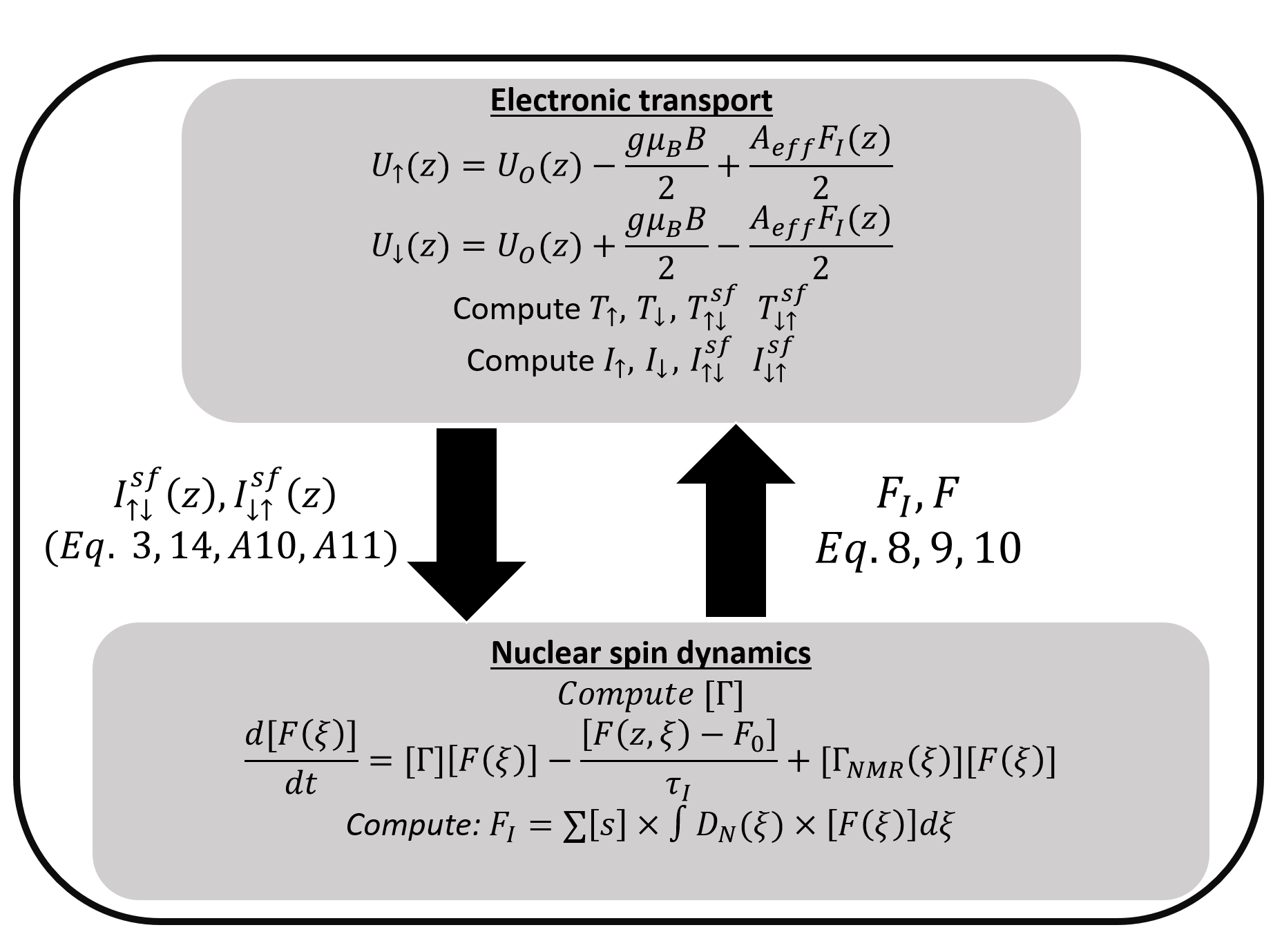
For a system with quad nuclear spin levels as in GaAs, it can be shown that $\Gamma_{\downarrow\uparrow}=C_{2}|I_{\downarrow\uparrow}^{sf}|$ and $\Gamma_{\uparrow\downarrow}=C_{1}|I_{\uparrow\downarrow}^{sf}|$ with $C_{1}=\frac{1}{qN_{I}\{1-F_{\frac{3}{2}}\}}$ and $C_{2}=\frac{1}{qN_{I}\{1-F_{-\frac{3}{2}}\}}$ (details given in Appendix C), $N_{I}$ being the number of nuclei that are being influenced by spin flip-flop processes at the QPC. We can hence rewrite the expression for $[\Gamma]$ as (details given in Appendix C):

$$\left[\Gamma\right]=\begin{bmatrix}-C_{2}|I_{\downarrow\uparrow}^{sf}|&C_{1}|I_{\uparrow\downarrow}^{sf}|&0&0\\ C_{2}|I_{\downarrow\uparrow}^{sf}|&-\left(C_{2}|I_{\downarrow\uparrow}^{sf}|+C_{1}|I_{\uparrow\downarrow}^{sf}|\right)&C_{1}|I_{\uparrow\downarrow}^{sf}|&0\\ 0&C_{2}|I_{\downarrow\uparrow}^{sf}|&-\left(C_{2}|I_{\downarrow\uparrow}^{sf}|+C_{1}|I_{\uparrow\downarrow}^{sf}|\right)&C_{1}|I_{\uparrow\downarrow}^{sf}|\\ 0&0&C_{2}|I_{\downarrow\uparrow}^{sf}|&-C_{1}|I_{\uparrow\downarrow}^{sf}|.\end{bmatrix}$$

(15)

Let us now consider the experimental features on a case by case basis.

We first reproduce some trends noted in the conductance plots of a recent experiment [3] where a change in the conductance along with hysteresis in the conductance was noted in the vicinity of $V=0$ with positive and negative source to drain voltage sweep. We explain the possible phenomena giving rise to such experimental trends.
Case I: $dI/dV<e^{2}/h$
A schematic of the scattering processes in this regime is shown in Fig. 3(a) while the up-spin and down-spin edge current paths and equivalent circuit models for the phenomena occuring around the QPC are shown in Fig. 5(a) and (b) respectively. In this case, the following points are to be noted:

1. 1.

   Only the up-spin channel is transmitted through the QPC.

2. 2.

   The down-spin channel originating in the source contact is totally reflected at the QPC.

3. 3.

   Some up-spin electrons in the edge channel terminating in the drain contact can scatter at the QPC to the down-spin edge channel terminating in the drain contact via electron-nuclear spin flip-flop scattering. Such a scattering decreases the current in the up-spin channel just outside the QPC and increases the current in the down-spin edge channel outside the QPC. However, the total current remains proportional to $T_{\uparrow}(E)$.

Reason for an increase in $dI/dV$ near $V=0$.

1. 1.

   Near V=0, the nuclear polarization cannot be maintained.

2. 2.

   Nuclear polarization drops due to spin lattice relaxation.

3. 3.

   A drop in nuclear polarization results in an increase in the direct transmission coefficient $T_{\uparrow}$ of the up-spin channel due to a decrease in the Overhauser field as well as an increase in the spin-flip transmission coefficient $T_{\uparrow\downarrow}^{sff}$.

Equivalent circuit model:
A schematic of the edge channel path in this case is shown in Fig. 5 (a) while the equivalent circuit in this case is detailed in Fig. 5 (b) to aid a visualization of the various transport phenomena inside the device. The circuit model can be described as follows:

1. 1.

   The up-spin edge channel is represented by a conductance $G=0.68\frac{e^{2}}{h}$.

2. 2.

   The up-to-down spin-flip scattering can be represented by an equivalent current source from the up-spin channel. $I_{UD}=0.01I_{U}\times\{1-F_{\frac{3}{2}}\}$.

3. 3.

   The change in transmissivity of the up-spin channel due to the Overhauser field is represented by a by an equivalent conductor $(G=0.02\frac{e^{2}}{h})$ in series with a voltage dependent voltage source $V_{p}=\frac{2}{3}F_{I}\times\{\mu_{S}-\mu_{D}\}$. The current change due to the Overhauser field is represented by $I_{U}^{Ov}$.

4. 4.

   The nuclear polarization is represented by the voltage across the capacitor.

5. 5.

   The resistance in parallel with the capacitor represents nuclear spin-lattice relaxation.

Case II $dI/dV>e^{2}/h$
A schematic of the scattering processes in this regime is shown in Fig. 3(b) while the up-spin and down-spin edge current paths and equivalent circuit models for the phenomena occuring around the QPC is shown in Fig. 5 (c) and (d) respectively. In this case, the following points are to be noted:

1. 1.

   The up-spin electrons in the edge channel originating in the source contact are fully transmitted through the QPC to the up-spin edge channel terminating in the drain contact.

2. 2.

   The down-spin electrons in the edge channel originating in the source contact are partially transmitted through the QPC to the down-spin edge channel terminating in the drain contact.

3. 3.

   Two kinds of electron-nuclear spin-flip scattering dominate at the QPC in this case:

   1. (a)

      Electrons from the forward propagating up-spin channel terminating in the drain contact can undergo spin-flip scattering to the forward propagating down-spin channel terminating in the drain contact which is almost empty in the energy range between $\mu_{S}$ and $\mu_{D}$. Such scattering at and around the QPC results in a positive nuclear polarization.

   2. (b)

      Electrons in forward propagating down-spin channel propagating through the QPC can undergo a spin-flip scattering to the backward propagating up-spin channel (which is totally empty in the energy range between $\mu_{S}$ and $\mu_{D}$) terminating in the source contact. Such scattering results in a negative nuclear polarization in addition to decreasing the total current through the QPC.

   3. (c)

      Out of these two processes, the former process dominates at the QPC due to the presence of more up-spin electrons compared to down-spin electrons resulting in a net positive nuclear polarization at the QPC.

Reason for a decrease in $dI/dV$ near $V=0$:

1. 1.

   Near $V=0$, the nuclear polarization cannot be maintained.

2. 2.

   Nuclear polarization drops due to spin-lattice relaxation.

3. 3.

   A drop in polarization results in an increase in the up-to-down spin-flip rate as well as a decrease in down-to-up spin-flip rate in addition to a decrease in the direct transmission coefficient $T_{\downarrow}$ of the down-spin channel due to decrease in the Overhauser field.

4. 4.

   The decrease in transmission coefficient of the down-spin channel decreases the conductance of the QPC in the vicinity of $V=0$.

Equivalent circuit model:
The equivalent circuit in this case is detailed in Fig. 5(d). The circuit model can be described as follows:

1. 1.

   The up spin edge channel originating in the source contact is fully transmitted through the QPC and hence is represented by a conductance $G=e^{2}/h$.

2. 2.

   The down-spin edge channel originating in the source contact is partially transmitted through the QPC to the down-spin edge channel terminating in the drain contact and hence is represented by a conductance $G=0.11\frac{e^{2}}{h}$.

3. 3.

   The up-to-down spin-flip current at the QPC from the forward propagating up-spin channel terminating in the drain contact to the forward propagating down-spin channel terminating in the drain contact is represented by a current dependent current source $I_{UD}=0.01I_{U}\times\{1-F_{\frac{3}{2}}\}$.

4. 4.

   The down-to-up spin-flip current from the forward propagating down-spin channel originating in the source contact to the backward propagating up-spin channel terminating in the source contact is represented by a current dependent current source $I_{DU}=0.01I_{D}\times\{1-F_{-\frac{3}{2}}\}$.

5. 5.

   The change in the transmission coefficient of the down-spin channel due to the Overhauser field is represented by a by an equivalent conductor $(G=0.02\frac{e^{2}}{h})$ in series with a voltage dependent voltage source ($V_{p}=\frac{2}{3}\{\frac{3}{2}-F_{I}\}\times\{\mu_{S}-\mu_{D}\}$). The current change due to the Overhauser field is represented by $I_{D}^{Ov}$.

6. 6.

   The nuclear polarization is represented by the voltage across the capacitor.

7. 7.

   The resistance in parallel with the capacitor represents nuclear spin-lattice relaxation by causing charge leakage from the capacitor.
   

We begin our analysis with (14), where the nuclear polarization in the vicinity of the QPC is perturbed by an externally applied alternating magnetic field in the radio frequency (RF) range resulting in the Zeeman split nuclear levels to interact with each other. Near the frequency corresponding to the difference in energy between the two spin split nuclear energy levels ($\hslash\omega=\xi_{s+1}-\xi_{s}$), precession of the nuclear spins accompanied by a rapid decay in the nuclear polarization occurs. To model such processes, we model the spin split nuclear energy levels by a broadened normalized density of states [39, 40, 31].

$$D_{s}(\xi)=\frac{1}{2\pi}\frac{\eta}{(\xi-\epsilon_{s})^{2}+(\frac{\eta}{2})^{2}},$$

where $\xi$ is the free variable denoting energy in the nuclear spin space, $\eta$ is related to the amount of broadening of the nuclear spin levels and $\epsilon_{s}$ is the energy level of the $s^{th}$ nuclear spin in the absence of broadening. Broadening might be a result of thermal motion of the nucleus [31], hyperfine interaction mediated electron-nuclear spin exchange [31] as well as nuclear dipole-dipole exchange interaction [31] which is the causative agent for nuclear spin diffusion[31]. We take broadening to be $\eta=10^{-4}\mu eV$. We simulate the case of quad nuclear spin levels, as in GaAs, separated in energy due to Zeeman splitting. The rate equations in this case are given by:

	$\displaystyle\left[\frac{dF(\xi)}{dt}\right]=\left[\frac{dF(\xi)}{dt}\right]_{flip-flop}$	$\displaystyle+\left[\frac{dF(\xi)}{dt}\right]_{relaxation}$
		$\displaystyle+\left[\frac{dF(\xi)}{dt}\right]_{NMR}$

$$F_{I}=\int^{\infty}_{-\infty}\left[s\right]\times[D_{N}(\xi)]\times\left[F(\xi)\right]d\xi$$

(17)

	$\displaystyle T_{\downarrow\uparrow}^{sff}(E)$	$\displaystyle=T_{\downarrow\uparrow}^{f}T_{\downarrow}(E)\{1-\int D_{-\frac{3}{2}}(\xi)F_{-\frac{3}{2}}(\xi)d\xi\}$
	$\displaystyle T_{\uparrow\downarrow}^{sff}(E)$	$\displaystyle=T_{\uparrow\downarrow}^{f}T_{\uparrow}(E)\{1-\int D_{\frac{3}{2}}(\xi)F_{\frac{3}{2}}(\xi)d\xi\}$
	$\displaystyle T_{\downarrow\uparrow}^{sfb}(E)$	$\displaystyle=T_{\downarrow\uparrow}^{b}T_{\downarrow}(E)\{1-\int D_{-\frac{3}{2}}(\xi)F_{-\frac{3}{2}}(\xi)d\xi\}$
	$\displaystyle T_{\uparrow\downarrow}^{sfb}(E)$	$\displaystyle=T_{\uparrow\downarrow}^{b}T_{\uparrow}(E)\{1-\int D_{\frac{3}{2}}(\xi)F_{\frac{3}{2}}(\xi)d\xi\}$

	$\displaystyle I_{\uparrow\downarrow}^{sf}=\int\frac{e}{h}\{T_{\uparrow\downarrow}^{sff}(E)+T_{\uparrow\downarrow}^{sfb}(E)\}\{f_{S}(E)-f_{D}(E)\}dE$
	$\displaystyle I_{\downarrow\uparrow}^{sf}=\int\frac{e}{h}\{T_{\downarrow\uparrow}^{sff}(E)+T_{\downarrow\uparrow}^{sfb}(E)\}\{f_{S}(E)-f_{D}(E)\}dE,$
			(19)

where $\left[s\right]=\left[\frac{3}{2}~~\frac{1}{2}~~-\frac{1}{2}~~-\frac{3}{2}\right]$ is the row vector denoting four nuclear spin levels in GaAs and $[F(\xi)]=\left[F_{\frac{3}{2}}(\xi)~~F_{\frac{1}{2}}(\xi)~~F_{-\frac{1}{2}}(\xi)~~F_{-\frac{3}{2}}(\xi)\right]^{\dagger}$. $F_{s}(\xi)$ is the probability of occupancy of the density of states of the $s^{th}$ nuclear spin level $D_{s}$ at energy $\xi$. The matrix $D_{N}(\xi)$ is the diagonal matrix representing the nuclear density of states at energy $\xi$ given by:

$$D_{N}(\xi)=\begin{bmatrix}D_{\frac{3}{2}}(\xi)&0&0&0\\ 0&D_{\frac{1}{2}}(\xi)&0&0\\ 0&0&D_{-\frac{1}{2}}(\xi)&0\\ 0&0&0&D_{-\frac{3}{2}}(\xi)\end{bmatrix}$$

At low temperatures, $\{f_{S}(E)-f_{D}(E)\}$ is a boxcar function. Assuming that the average value of $T_{\uparrow}$ and $T_{\downarrow}$ in the energy range between $\mu_{S}$ and $\mu_{D}$ are $T_{\uparrow}^{avg}$ and $T_{\downarrow}^{avg}$ respectively and the spin-flip transmission coefficients, $T_{\uparrow\downarrow}^{f(b)}$ and $T_{\downarrow\uparrow}^{f(b)}$, are constant in the range of energy between $\mu_{S}$ and $\mu_{D}$, the above equation can be simplified to,

	$\displaystyle I_{\uparrow\downarrow}^{sf}=\frac{e}{h}T_{\uparrow}^{avg}\{T_{\uparrow\downarrow}^{f}+T_{\uparrow\downarrow}^{b}\}\times\{1-\int D_{\frac{3}{2}}(\xi)F_{\frac{3}{2}}(\xi)d\xi\}\Delta\mu$
	$\displaystyle=\frac{e^{2}}{h}T_{\uparrow}^{avg}T_{\uparrow\downarrow}^{avg}\times\{1-\int D_{\frac{3}{2}}(\xi)F_{\frac{3}{2}}(\xi)d\xi\}V$
	$\displaystyle I_{\downarrow\uparrow}^{sf}=\frac{e}{h}T_{\downarrow}^{avg}\{T_{\downarrow\uparrow}^{f}+T_{\downarrow\uparrow}^{b}\}\times\{1-\int D_{-\frac{3}{2}}(\xi)F_{-\frac{3}{2}}(\xi)d\xi\}\Delta\mu$
	$\displaystyle=\frac{e^{2}}{h}T_{\downarrow}^{avg}T_{\downarrow\uparrow}^{avg}\times\{1-\int D_{-\frac{3}{2}}(\xi)F_{-\frac{3}{2}}(\xi)d\xi\}V,$
			(20)

where $\Delta\mu=\mu_{S}-\mu_{D}$. The set of equations ()-(19) have to be solved self-consistently to calculate the temporal evolution of the nuclear polarization. We now turn our attention towards (). The first term on the right hand side of () is given by:

$$\left[\frac{dF(\xi)}{dt}\right]_{flip-flop}=\left[\Gamma_{out}\right]\times[F(\xi)]\\ +\{[I_{4}]-[F_{diag}(\xi)]\}\times[P_{diag}]^{-1}\left[\Gamma_{in}\right][N],$$

(21)

where $I_{4}$ is the identity matrix of the fourth order and [$N_{diag}$], [$P_{diag}$], $\left[\Gamma_{in}\right]$ and $\left[\Gamma_{out}\right]$ are given by:

$$[F_{diag}(\xi)]=\begin{bmatrix}F_{\frac{3}{2}}(\xi)&0&0&0\\ 0&F_{\frac{1}{2}}(\xi)&0&0\\ 0&0&F_{-\frac{1}{2}}(\xi)&0\\ 0&0&0&F_{-\frac{3}{2}}(\xi)\end{bmatrix}$$

(22)

$$[N]=\int\left[D_{\frac{3}{2}}(\xi)F_{\frac{3}{2}}(\xi)~~D_{\frac{1}{2}}(\xi)F_{\frac{1}{2}}(\xi)~~D_{-\frac{1}{2}}(\xi)F_{-\frac{1}{2}}(\xi)~~D_{-\frac{3}{2}}(\xi)F_{-\frac{3}{2}}(\xi)\right]^{\dagger}d\xi$$

(23)

$$P_{diag}=\begin{bmatrix}\int D_{\frac{3}{2}}(\xi)\{1-F_{\frac{3}{2}}(\xi)\}d\xi&0&0&0\\ 0&\int D_{\frac{1}{2}}(\xi)\{1-F_{\frac{1}{2}}(\xi)\}d\xi&0&0\\ 0&0&\int D_{-\frac{3}{2}}(\xi)\{1-F_{-\frac{3}{2}}(\xi)\}d\xi&0\\ 0&0&0&\int D_{-\frac{3}{2}}(\xi)\{1-F_{-\frac{3}{2}}(\xi)\}d\xi\end{bmatrix}$$

(24)

$$\left[\Gamma_{in}\right]=\begin{bmatrix}0&C_{1}|I_{\uparrow\downarrow}^{sf}|&0&0\\ C_{2}|I_{\downarrow\uparrow}^{sf}|&0&C_{1}|I_{\uparrow\downarrow}^{sf}|&0\\ 0&C_{2}|I_{\downarrow\uparrow}^{sf}|&0&C_{1}|I_{\uparrow\downarrow}^{sf}|\\ 0&0&C_{2}|I_{\downarrow\uparrow}^{sf}|&0.\end{bmatrix}$$

(25)

References

- [1] Y. Hirayama, G. Yusa, K. Hashimoto, N. Kumada, T. Ota, and K. Muraki, Semiconductor Science and Technology 24, 023001 (2009).
- [2] B. Urbaszek, X. Marie, T. Amand, O. Krebs, P. Voisin, P. Maletinsky, A. Högele, and A. Imamoglu, Rev. Mod. Phys. 85, 79 (2013).
- [3] K. R. Wald, L. P. Kouwenhoven, P. L. McEuen, N. C. van der Vaart, and C. T. Foxon, Phys. Rev. Lett. 73, 1011 (1994).
- [4] T. Machida, T. Yamazaki, and S. Komiyama, Applied Physics Letters 80, 4178 (2002).
- [5] T. Machida, T. Yamazaki, K. Ikushima, and S. Komiyama, Applied Physics Letters 82, 409 (2003).
- [6] A. Würtz, T. Müller, A. Lorke, D. Reuter, and A. D. Wieck, Phys. Rev. Lett. 95, 056802 (2005).
- [7] Y. Ren, W. Yu, S. M. Frolov, J. A. Folk, and W. Wegscheider, Phys. Rev. B 81, 125330 (2010).
- [8] C. R. Dean, B. A. Piot, G. Gervais, L. N. Pfeiffer, and K. W. West, Phys. Rev. B 80, 153301 (2009).
- [9] A. M. Song and P. Omling, Phys. Rev. Lett. 84, 3145 (2000).
- [10] M. Kawamura, H. Takahashi, K. Sugihara, S. Masubuchi, K. Hamaya, and T. Machida, Applied Physics Letters 90, 022102 (2007).
- [11] Z. K. Keane, M. C. Godfrey, J. C. H. Chen, S. Fricke, O. Klochan, A. M. Burke, A. P. Micolich, H. E. Beere, D. A. Ritchie, K. V. Trunov, D. Reuter, A. D. Wieck, and A. R. Hamilton, Nano Letters 11, 3147 (2011a).
- [12] K. Hashimoto, K. Muraki, T. Saku, and Y. Hirayama, Phys. Rev. Lett. 88, 176601 (2002).
- [13] A. Kou, D. T. McClure, C. M. Marcus, L. N. Pfeiffer, and K. W. West, Phys. Rev. Lett. 105, 056804 (2010).
- [14] K. Akiba, S. Kanasugi, K. Nagase, and Y. Hirayama, Applied Physics Letters 99, 112106 (2011).
- [15] K. Akiba, T. Yuge, S. Kanasugi, K. Nagase, and Y. Hirayama, Phys. Rev. B 87, 235309 (2013).
- [16] T. Hatano, W. Kume, S. Watanabe, K. Akiba, K. Nagase, and Y. Hirayama, Phys. Rev. B 91, 115318 (2015).
- [17] M. Kawamura, T. Yamashita, H. Takahashi, S. Masubuchi, Y. Hashimoto, S. Katsumoto, and T. Machida, Applied Physics Letters 96, 032102 (2010).
- [18] G. Gervais, “Resistively detected nmr in gaas/algaas,” in Electron Spin Resonance and Related Phenomena in Low-Dimensional Structures, edited by M. Fanciulli (Springer Berlin Heidelberg, Berlin, Heidelberg, 2009) pp. 35–50.
- [19] C. R. Bowers, G. M. Gusev, J. Jaroszynski, J. L. Reno, and J. A. Simmons, Phys. Rev. B 81, 073301 (2010).
- [20] Z. K. Keane, M. C. Godfrey, J. C. H. Chen, S. Fricke, O. Klochan, A. M. Burke, A. P. Micolich, H. E. Beere, D. A. Ritchie, K. V. Trunov, D. Reuter, A. D. Wieck, and A. R. Hamilton, Nano Letters 11, 3147 (2011b).
- [21] L. Tiemann, T. D. Rhone, N. Shibata, and K. Muraki, Nat Phys 10, 648 (2014), letter.
- [22] K. F. Yang, H. W. Liu, T. D. Mishima, M. B. Santos, K. Nagase, and Y. Hirayama, Journal of Physics: Conference Series 334, 012029 (2011).
- [23] K. Kodera, H. Takado, A. Endo, S. Katsumoto, and Y. Iye, physica status solidi (c) 3, 4380 (2006).
- [24] L. A. Tracy, J. P. Eisenstein, L. N. Pfeiffer, and K. W. West, Phys. Rev. B 73, 121306 (2006).
- [25] W. Desrat, D. K. Maude, M. Potemski, J. C. Portal, Z. R. Wasilewski, and G. Hill, Phys. Rev. Lett. 88, 256807 (2002).
- [26] G. Gervais, H. L. Stormer, D. C. Tsui, P. L. Kuhns, W. G. Moulton, A. P. Reyes, L. N. Pfeiffer, K. W. Baldwin, and K. W. West, Phys. Rev. Lett. 94, 196803 (2005).
- [27] M. P. Zaletel, R. S. K. Mong, F. Pollmann, and E. H. Rezayi, Phys. Rev. B 91, 045115 (2015).
- [28] J. Sakurai and J. Napolitano, Modern Quantum Mechanics (Addison-Wesley, 2011).
- [29] J. Sakurai and J. Napolitano, Advanced Quantum Mechanics (Addison-Wesley, 2011).
- [30] D. Griffiths, Introduction to Quantum Mechanics, Pearson international edition (Pearson Prentice Hall, 2005).
- [31] C. P. Slichter, Principles of Magnetic Resonance (Springer-Verlag Berlin Heidelberg, 1990).
- [32] S. Das Sarma, E. H. Hwang, and A. Kaminski, Phys. Rev. B 67, 155201 (2003).
- [33] S. Buddhiraju and B. Muralidharan, Journal of Physics: Condensed Matter 26, 485302 (2014).
- [34] L. Siddiqui, A. N. M. Zainuddin, and S. Datta, Journal of Physics: Condensed Matter 22, 216002 (2010).
- [35] S. Salahuddin, Novel electronic and spintronic devices for low power logic computation, Ph.D. thesis, Purdue University (2006).
- [36] M. Kawamura, K. Ono, P. Stano, K. Kono, and T. Aono, Phys. Rev. Lett. 115, 036601 (2015).
- [37] J. Wan, M. Cahay, P. Debray, and R. Newrock, Phys. Rev. B 80, 155440 (2009).
- [38] R. Côté and A. M. Simoneau, Phys. Rev. B 93, 075305 (2016).
- [39] S. Datta, Electronic Transport in Mesoscopic Systems (Cambridge University Press, 1997).
- [40] S. Datta, Quantum Transport: Atom to Transistor (Cambridge press, 2005).
- [41] S. Datta, Lessons from nanoelectronics: a new perspective on transport. (World Scientific, 2012).
- [42] G. Yusa, K. Muraki, K. Takashina, K. Hashimoto, and Y. Hirayama, Nature 434, 1001 (2005).
- [43] Y. Hirayama, A. Miranowicz, T. Ota, G. Yusa, K. Muraki, S. K. Ozdemir, and N. Imoto, Journal of Physics: Condensed Matter 18, S885 (2006).
- [44] A. Miranowicz, i. m. c. K. Özdemir, J. c. v. Bajer, G. Yusa, N. Imoto, Y. Hirayama, and F. Nori, Phys. Rev. B 92, 075312 (2015).
- [45] D. B. Chklovskii, B. I. Shklovskii, and L. I. Glazman, Phys. Rev. B 46, 4026 (1992).
- [46] A. Yacoby, T. A. Fulton, H. F. Hess, L. N. Pfei, and K. W. West, Physica E: Low-dimensional Systems and Nanostructures, 9, 40 (2001).
- [47] J. H. Oh and R. R. Gerhardts, Phys. Rev. B 56, 13519 (1997).
- [48] K. Güven and R. R. Gerhardts, Phys. Rev. B 67, 115327 (2003).
- [49] A. Siddiki, arXiv:arXiv:0707.1123v1 .
- [50] E. Papa and T. Stroh, Phys. Rev. B 75, 045342 (2007).
- [51] A. L. Efros, Phys. Rev. B 60, 13343 (1999).
- [52] R. R. Gerhardts, physica status solidi (b) 245, 378 (2008).
- [53] C. L. Kane and M. P. A. Fisher, Edge state transport.
- [54] J. R. Nikolajsen, Edge States and Contacts in the Quantum Hall Effect (2013).
- [55] R. R. Gerhardts, K. Panos, and J. Weis, New Journal of Physics 15, 073034 (2013).
- [56] S. Arslan, E. Cicek, D. Eksi, S. Aktas, A. Weichselbaum, and A. Siddiki, Phys. Rev. B 78, 125423 (2008).