Quelques contributions à la théorie de l’action de sur les espaces de modules de surfaces plates
Remerciements
Je dédie ce mémoire à Jean-Christophe Yoccoz : son amitié et bienveillance envers moi après mon arrive en France en 2007 ont marqué ma vie (mathématique et personnelle) à jamais, et je lui serai toujours reconnaissant.
Je remercie Yves Benoist, Stefano Marmi et Anton Zorich d’avoir accepté de relire mon mémoire et d’écrire les rapports à son sujet, et Julien Barral, Henry de Thélin et Giovanni Forni pour me faire l’honneur d’être membres de jury d’examen de ce mémoire.
Je remercie aussi mes coauteurs pour avoir partager avec moi la joie de la découverte de nouveaux théorèmes.
À Aline et Marie-Inès, “la reine et la princesse de mon château à Fontainebleau–Avon”, et à Dominique et Véronique pour toute leur amitié.
Description du mémoire
Ce mémoire est basé sur certains de mes travaux autour de la dynamique de Teichmüller ou, plus précisément, la dynamique de l’action de sur les espaces de modules de surfaces plates.
Le chapitre 1 sert à introduire plusieurs aspects classiques de la dynamique de Teichmüller. Son contenu est inspiré par les survols de Zorich [71] et Yoccoz [69], ainsi que les notes [31] d’un minicours donné par Forni et moi-même en 2011 au Banach Center (Bedlewo, Pologne). En particulier, ce chapitre est une introduction générale à tous les chapitres postérieurs, de façon qu’on va toujours supposer une certaine familiarité avec ce chapitre dans toutes les discussions dans d’autres chapitres.
Après avoir lu le premier chapitre, le lecteur peut choisir librement quel ordre suivre pour la lecture de chapitre restants : en fait, les résultats discutés dans les chapitres 2 à 6 sont complètement indépendants les uns des autres.
Le chapitre 2 traite de la régularité des mesures -invariantes sur les espaces de modules de surfaces plates. En général, une telle mesure est dite régulière si la plupart des surfaces plates dans son support possèdent leurs connexions de selles plus courts parallèles entre eux. La propriété de régularité a été utilisée par Eskin, Kontsevich et Zorich [19] pour justifier un argument sophistiqué d’intégration par parties intervenant dans la démonstration de leur célèbre formule pour la somme des exposants de Lyapunov non-négatifs du cocycle de Kontsevich-Zorich (la partie intéressante de la dérivée de l’action de sur les surfaces plates). Dans ce même article, Eskin-Kontsevich-Zorich [19] ont conjecturé que la propriété de régularité est toujours valide, de façon que leur formule pour la somme des exposants de Lyapunov pourrait être appliquée sans exception à toutes les mesures de probabilité -invariantes ergodiques sur les espaces de modules de surfaces plates. Let but du chapitre 2 est discuter notre article [5] avec Avila et Yoccoz contenant une réponse affirmative à la conjecture de régularité d’Eskin-Kontsevich-Zorich.
Le chapitre 3 est consacré à l’étude de la vitesse de mélange du flot de Teichmüller. La question de la vitesse de decroissance des correlations pour les mesures de Masur-Veech a été résolu dans un célèbre article de Avila, Gouëzel et Yoccoz [4] : la vitesse de mélange du flot de Teichmüller par rapport à ces mesures est toujours exponentielle. Puis, Avila et Gouëzel [3] ont étendu le résultat d’Avila-Gouëzel-Yoccoz à toutes les mesures de probabilité -invariantes ergodiques sur les espaces de modules de surfaces plates. Une question naturelle motivée par les résultats d’Avila, Gouëzel et Yoccoz est savoir si la vitesse exponentielle de mélange de ces mesures est uniforme. Le résultat principal du chapitre 3 est un théorème obtenu en collaboration avec Schmithüsen [49] selon lequel il n’y a pas d’uniformité sur la vitesse exponentielle de mélange de telles mesures lorsqu’on regarde des espaces de modules de surfaces plates de genre arbitrairement grand.
Le chapitre 4 aborde le problème de classification des adhérences des -orbites dans les espaces de modules de surfaces plates. De nombreuses applications de la dynamique de Teichmüller à l’étude des billards mathématiques dépendent d’une connaissance précise des fermetures de certaines -orbites de surfaces plates, ce qui explique une partie de l’intérêt en classifier ces objets. Les résultats remarquables d’Eskin-Mirzakhani [22], Eskin-Mirzakhani-Mohammadi [23] et Filip [24] disent que les fermetures des -orbites des surfaces plates sont affines dans les coordonnées de périodes, quasi-projectives dans les coordonnées induites par les espaces de modules de courbes et leur totalité est une collection dénombrable : en particulier, il est raisonnable d’essayer de les classifier. Les travaux de Calta [11] et McMullen [54] fournissent une classification très satisfaisante des adhérences de -orbites de surfaces plates de genre deux. Par contre, la situation en genre supérieur n’est toujours pas complètement comprise malgré les nombreux progrès partiels récents. Néamoins, cette situation semble s’amérioler un peu lorsqu’on se concentre sur les courbes de Teichmüller (i.e., les -orbites fermées) : par exemple, Bainbridge, Habegger et Möller [9] ont prouvé la finitude des courbes de Teichmüller algébriquement primitives engendrées par des surfaces plates de genre trois. Dans le chapitre 4, on discutera un résultat obtenu avec Wright [51] assurant la finitude des courbes de Teichmüller algébriquement primitives engendrées par des surfaces plates de genre premier ayant une seule singularité conique.
Le chapitre 5 examine les exposants de Lyapunov du cocycle de Kontsevich-Zorich (la partie intéressante de la dérivée de l’action de sur les surfaces plates). Les propriétés qualitatives et/ou quantitatives des exposants de Lyapunov du KZ cocycle jouent un rôle important dans de nombreuses applications de la dynamique de Teichmüller : par exemple, Avila et Forni [2] ont exploré le résultat de Forni [28] de hyperbolicité non-uniforme du cocycle de KZ par rapport aux mesures de Masur-Veech pour montrer que les transformations d’échange d’intervalles typiques (qui ne sont pas des rotations) sont faiblement mélangeantes. D’un point de vue qualitatif, les exposants de Lyapunov du KZ cocycle par rapport aux mesures de Masur-Veech sont bien compris grâce à un célèbre article d’Avila et Viana [6] assurant la simplicité (i.e., multiplicité un) de ces exposants (confirmant donc une conjecture de Kontsevich et Zorich). Par contre, ceci n’est plus vrai pour d’autres mesures : Forni et moi-même (voir [31] par exemple) avons deux exemples de mesures de probabilités -invariantes sur les espaces de modules de surfaces plates pour lequelles les exposants de Lyapunov du cocycle KZ sont loin d’être simples. Du coup, il est intéressant de savoir en général dans quelles conditions les exposants de Lyapunov du cocycle KZ sont simples. Le point de départ du chapitre 5 est un résultat obtenu en collaboration avec Eskin [21] assurant que les exposants de Lyapunov du KZ cocycle sur les courbes de Teichmüller (-orbites fermées) peuvent être calculés à l’aide de produits de matrices aléatoires. Ensuite, ce résultat et les techniques d’Avila et Viana [6] sont exploités pour fournir un critère efficace (basé sur la théorie de Galois) obtenu en collaboration avec Möller et Yoccoz [50] pour la simplicité des exposants de Lyapunov de KZ cocycle sur les courbes de Teichmüller arithmétiques. Enfin, ce critère de type Galois pour la simplicité est utilisé dans la discussion d’un contre-exemple dû à Delecroix et moi-même [15] à une conjecture de Forni.
Le chapitre 6 est dédié à la structure du groupe de matrices associé au cocycle de Kontsevich-Zorich (i.e., la partie intéressante de la dérivée de l’action de dans les espaces de modules de surfaces plates). Les groupes de matrices engendrés par le cocycle KZ méritent une attention particulière car ils ont un rôle clé dans l’étude de l’action de sur les surfaces plates : par exemple, le célèbre travail d’Eskin-Mirzakhani [22] sur la classification des mesures -invariantes dans les espaces de modules de surfaces plates est basé sur une analyse fine de ce cocycle. Un travail récent de Filip [26] fournit une liste de toutes les adhérences de Zariski possibles (modulo facteurs compacts et à indice fini près) pour les groupes de matrices associés au cocycle KZ : en particulier, Filip a confirmé une conjecture de Forni, Zorich et moi-même [33] sur l’origine des exposants de Lyapunov nuls pour le cocycle KZ. Cependant, la liste de Filip est produite à partir de considérations de variations de structures de Hodge sur les variétés quasi-projectives et, par conséquent, une question naturelle est de savoir quels groupes de la liste apparaissent effectivement dans le contexte du cocycle KZ. Le résultat principal du chapitre 6 est un exemple de Filip, Forni et moi-même [27] montrant que l’un des groupes de matrices quaternioniques dans la liste Filip est réalisé dans le cadre du cocycle KZ.
Enfin, les limites habituelles de l’espace et du temps m’ont forcé à laisser quelques aspects de mon travail en dehors de ce texte. Par exemple, les sujets suivants mentionnés dans la liste des publications de l’auteur ne seront pas discutés ici :
- —
les articles (MY) (avec Yoccoz), (FMZi), (FMZii) et (FMZiii) (avec Forni et Zorich), (MYZ) (avec Yoccoz et Zmiaikou), (MSch) (avec Schmithüsen) sur la dynamique de Teichmüller,
- —
les articles (BMMWi) et (BMMWii) (avec Burns, Masur et Wilkinson) sur la vitesse de mélange du flot de Weil-Petersson sur les espaces de modules de surfaces hyperboliques,
- —
les articles (MMP) (avec Moreira et Pujals), (M), (CMM) (avec Cerqueira et Moreira), (LM) (avec Lima) sur la dynamique en basse dimension, et
- —
les articles (ACM) (avec Arbieto et Corcho), (M07), (AM) (avec Arbieto), (LM09) (avec Linares), (CM09) (avec Corcho) et (AMP) (avec Angulo et Pilod) sur les EDPs dispersives.
Liste de publications de l’auteur
Articles de recherche (après la thèse de doctorat)
- (ACM)
Rough solutions for the periodic Schrödinger-Korteweg-deVries system, avec A. Arbieto et Adán Corcho. Journal of Differential Equations, vol.230, p.295-336 (2006).
- (M07)
Global well-posedness of NLS-KdV systems for periodic functions, Electronic Journal of Differential Equations, vol. 2007, p. 1-20 (2007).
- (AM)
On the periodic Schrödinger-Debye equation, avec A. Arbieto, Communications in Pure and Applied Analysis, vol. 7, p. 699-713 (2008).
- (LM09)
Well-posedness for the 1D Zakharov-Rubenchik system, avec Felipe Linares, Advances in Differential Equations, vol. 14, n.3-4, 261-288 (2009).
- (CM09)
Sharp bilinear estimates and well-posedness for the 1D Schrödinger-Debye system, avec Adán Corcho, Differential and Integral Equations, vol. 22, n.3-4, 357-391 (2009).
- (AMP)
Global well-posedness and non-linear stability of periodic traveling waves for a Schrödinger-Benjamin-Ono system, avec Jaime Angulo et Didier Pilod, Communications in Pure and Applied Analysis, vol. 8, n.3, 815-844 (2009).
- (MY)
The action of the affine diffeomorphisms on the relative homology group of certain exceptionally symmetric origamis, avec Jean-Christophe Yoccoz, Journal of Modern Dynamics, vol. 4, n.3, 453-486 (2010).
- (FMZi)
Square-tiled cyclic covers, avec Giovanni Forni et Anton Zorich, Journal of Modern Dynamics, vol. 5, n.2, 285-318 (2011).
- (M11)
Other relevant examples : annexe à l’article “A geometric criterion for the non-uniform hyperbolicity of the Kontsevich-Zorich cocycle” de G. Forni, Journal of Modern Dynamics, vol. 5, n.2, 355-395 (2011).
- (M)
Some quantitative versions of Ratner’s mixing estimates, Bulletin Brazilian Mathematical Society, vol. 44, 469-488 (2013).
- (AMY)
-invariant probability measures on the moduli spaces of translation surfaces are regular, avec Artur Avila et Jean-Christophe Yoccoz, Geometric and Functional Analysis, v. 23, p. 1705-1729 (2013).
- (MMP)
Axiom A versus Newhouse phenomena for Benedicks-Carleson toy models, avec Carlos Gustavo Moreira et Enrique Pujals, Annales Scientifiques de l’École Normale Supérieure, vol. 46, n. 6, p. 857-878 (2013).
- (MS)
Explicit Teichmüller curves with complementary series, avec Gabriela Weitze-Schmithüsen, Bulletin de la Société Mathématique de France, vol. 141, n. 4, 557-602 (2013).
- (FMZii)
Lyapunov spectrum of invariant subbundles of the Hodge bundle, avec Giovanni Forni et Anton Zorich, Ergodic Theory and Dynamical Systems, vol. 34, n. 2, 353-408 (2014).
- (FMZiii)
Zero Lyapunov exponents of the Hodge bundle, avec Giovanni Forni et Anton Zorich, Commentarii Mathematici Helvetici, vol. 89, n. 2, 489-535 (2014).
- (MYZ)
Homology of origamis with symmetries, avec Jean-Christophe Yoccoz et David Zmiaikou, Annales de l’Institut Fourier, vol. 64, 1131-1176 (2014).
- (DM)
Un contre-exemple à la réciproque du critère de Forni pour la positivité des exposants de Lyapunov du cocycle de Kontsevich-Zorich, avec Vincent Delecroix, Mathematical Research Letters, vol. 22, n. 6, 1667–1678 (2015)
- (EM)
A coding-free simplicity criterion for the Lyapunov exponents of Teichmüller curves, avec Alex Eskin, Geometriae Dedicata, vol. 179, n. 1, 45-67 (2015).
- (MW)
Hodge-Teichmüller planes and finiteness results for Teichmüller curves, avec Alex Wright, Duke Mathematical Journal, vol. 164, 1041-1077 (2015).
- (MSch)
Some examples of isotropic SL(2,R)-invariant subbundles of the Hodge bundle, avec Gabriela Weitze-Schmithüsen, International Mathematics Research Notices, vol. 2015, n. 18, 8657-8679 (2015).
- (MMY)
A criterion for the simplicity of the Lyapunov spectrum of square-tiled surfaces, avec Martin Möller et Jean-Christophe Yoccoz, Inventiones mathematicae, vol. 202, n. 1, 333-425 (2015).
- (FFM)
Quaternionic covers and monodromy of the Kontsevich-Zorich cocycle in orthogonal groups, avec Giovanni Forni et Simion Filip, à paraître dans Journal of the European Mathematical Society (2015).
- (BMMWi)
Rates of mixing for the Weil-Petersson geodesic flow I : no rapid mixing in non-exceptional moduli spaces, avec Keith Burns, Howard Masur et Amie Wilkinson. Prépublication (2015) disponible sur arXiv :1312.6012.
- (CMM)
Continuity of Hausdorff dimension across generic dynamical Lagrange and Markov spectra, avec Aline Cerqueira et Carlos Gustavo Moreira. Prépublication (2016) disponible sur arXiv :1602.04649.
- (BMMWii)
Rates of mixing for the Weil-Petersson geodesic flow II : exponential mixing in exceptional moduli spaces, avec Keith Burns, Howard Masur et Amie Wilkinson. Prépublication (2016) disponible sur arXiv :1605.09037.
- (AMYii)
Zorich conjecture for hyperelliptic Rauzy-Veech groups, avec Artur Avila et Jean-Christophe Yoccoz. Prépublication (2016) disponible sur arXiv :1606.01227.
- (LM)
Symbolic dynamics for non-uniformly hyperbolic surface maps with discontinuities, avec Yuri Lima. Prépublication (2016) disponible sur arXiv :1606.05863.
Articles de survol
- —
density of hyperbolicity for Benedicks-Carleson toy models, avec Carlos Gustavo Moreira et Enrique Pujals, Oberwolfach Reports, vol. 6, p. 1819-1823 (2009).
- —
On the neutral Oseledets bundle of Kontsevich-Zorich cocycle over certain cyclic covers, avec Giovanni Forni et Anton Zorich, Oberwolfach Reports, vol. 8, p. 1361-1427 (2011).
- —
Le flot géodésique de Teichmüller et la géométrie du fibré de Hodge, Actes du Séminaire de Théorie Spectrale et Géométrie du Institut Fourier à Grenoble, vol. 29, p. 73-95 (2010-2011).
- —
Fractal geometry of non-uniformly hyperbolic horseshoes, Proceedings of the Ergodic Theory Workshops at University of North Carolina at Chapel Hill, 2011-2012, Ed. by Idris Assani, p. 197-240 (2013).
- —
A criterium for the simplicity of Lyapunov exponents of origamis, avec Martin Möller et Jean-Christophe Yoccoz, Oberwolfach Reports, vol. 10, p. 1975–2033 (2013).
- —
Introduction to Teichmüller theory and its applications to dynamics of interval exchange transformations, flows on surfaces and billiards, avec Giovanni Forni, Journal of Modern Dynamics, vol. 8, no. 3/4, p. 271-436 (2014).
- —
Lecture notes on the dynamics of the Weil-Petersson flow, notes d’un minicours donné en novembre 2013 au CIRM, Marseille, à paraître dans CIRM Jean-Morlet Chair Subseries, Springer (2015).
- —
Variations of Hodge structures, Lyapunov exponents and Kontsevich’s formula, annexe à la monographie “Gauss-Manin Connection in Disguise (Calabi-Yau Modular Forms)” de Hossein Movasati, à paraître dans Surveys of Modern Mathematics, International Press, Boston (2016).
- —
Les blogs : un outil dynamique de communication en mathématiques, Gaz. Math. No. 148 (2016), 46–50.
Livres
- —
Aspectos ergódicos da teoria dos números (Ergodic aspects of Number Theory), joint with A. Arbieto and Carlos Gustavo Moreira, Publicações Matemáticas do IMPA - Colóquio Brasileiro de Matemática (2007).
- —
The remarkable efectiveness of Ergodic Theory in Number Theory, Parts I and II, (Part I together with A. Arbieto and Carlos Gustavo Moreira), Ensaios Matématicos vol. 17, p. 1-106 (2009).
1. Introduction
This section serves as a general-purpose introduction to all other sections of this memoir. In particular, we’ll always assume familiarity with the content of this section in subsequent discussions.
The basic references for this section are the survey texts of Zorich [71], Yoccoz [69], and Forni and the author [31].
1.1. Abelian differentials and their moduli spaces
Let be the set of Abelian differentials on a Riemann surface of genus , that is, the set of pairs where is a compact topological surface of genus and is a non-trivial -form which is holomorphic with respect to the underlying Riemann surface structure.
The Teichmüller space of Abelian differentials of genus is the quotient and the moduli space of Abelian differentials of genus is the quotient . Here is the set of diffeomorphisms isotopic to the identity and is the mapping class group (i.e., the set of isotopy classes of orientation-preserving diffeomorphisms), and both and act on the set of Riemann surface structure in the usual manner11 1 By precomposition with coordinate charts., while they act on Abelian differentials by pull-back.
Before equipping and with nice structures, let us give a concrete description of Abelian differentials in terms of translation structures.
1.2. Translation structures
Let and denote by the set of singularities of , or, equivalently, the divisor of , i.e., the finite set
For each , let us select a small simply-connected neighborhood of such that . In this context, the “period” map , given by integration along any path inside joining and is well-defined: in fact, any holomorphic -form is closed and, thus, the integral does not depend on the choice of the path inside connecting and . Furthermore, since (i.e., ), we have that, after reducing if necessary, this “period” map is a biholomorphism.
In other words, the collection of all such “period” maps is an atlas of which is compatible with the Riemann surface structure. By definition, the local expression of Abelian differential in these coordinates is (on ). Also, the local equality implies that all coordinate changes are where is a constant independent of . Moreover, since is finite, Riemann’s theorem on removable singularities implies that this atlas of “period” charts on can be extended to in such a way that the local expression of in a chart around a zero of of order is the holomorphic -form .
In the literature, a maximal atlas of compatible charts on the complement of a finite subset of a surface whose changes of coordinates are translations of the complex plane is called a translation structure on . In this language, the discussion in the previous paragraph says that determines a translation structure on . On the other hand, it is clear that a translation structure on determines a Riemann surface structure22 2 Since translations are particular cases of biholomorphisms. and an Abelian33 3 We define by locally pulling-back via the charts: this gives a globally defined Abelian differential because the changes of coordinates are translations and, hence, is invariant under changes of coordinates. differential on .
In summary, we proved the following proposition.
Proposition 1.
The set of all non-trivial Abelian differentials on compact Riemann surfaces of genus is canonically identified to the set of all translation structures on the compact surfaces of genus .
1.3. Some examples of translation surfaces
The notion of translation structures allows us to exhibit many concrete examples of Abelian differentials.
1.3.1. Abelian differentials on complex torus
We usually learn the concept of complex torii through translation structures. Indeed, a complex torus is the quotient of the complex plane by a lattice . These complex torii come equipped with Abelian differentials induced by on and they are usually depicted as a parallelogram of sides and whose parallel sides are identified via the translations and : see Figure 1.
1.3.2. Square-tiled surfaces
We can build more translation surfaces from certain coverings of the unit square torus equipped with the Abelian differential induced by .
More precisely, consider a finite collection of unit squares of the complex plane and let us glue by translations the leftmost, resp. bottomost, side of each square with the rightmost, resp. topmost, side of another (maybe the same) square . Here, we assume that, after performing the identifications, the resulting surface is connected.
In this way, we obtain a translation surface, namely, a Riemann surface with an Abelian differetianl (equal to on each square ). For obvious reasons, these translation surfaces are called square-tiled surfaces and/or origamis.
In Figure 2 we drew a -shaped square-tiled surface built up from three unit squares by identification (via translations) of pairs of sides with the same markings.
Remark 2.
The translation surface in Figure 2 has genus two. In fact, the corners of all squares are identified to a single point . Moreover, this point is special when compared to any other point because we have a total angle of by turning around (instead of a total angle of around all other points). In other terms, a neighborhood of looks like copies of the flat complex plane stitched together, that is, the natural local coordinate around is . In particular, the Abelian differential associated to this translation surface has the form near , i.e., has single zero of order two on . By Riemann-Hurwitz theorem, this means that where is the genus of , that is, has genus two44 4 Alternatively, this fact can be derived from Poincaré-Hopf index theorem applied to the vector field given by the vertical direction at all points of .
1.3.3. Suspensions of interval exchange transformations
We find translation surfaces during the construction of natural extensions of one-dimensional dynamical systems called interval exchange transformations. More concretely, recall that an interval exchange transformation (i.e.t.) of intervals is a map where are subsets of an open bounded interval with and the restriction of to each connected component of is a translation onto a connected component of : see Figure 3 for some examples.

It is possible to suspend (in several ways) any given i.e.t. to obtain translation flows55 5 A translation flow is obtained by moving (almost all) points of a translation surface in a fixed direction. on translation surfaces such that is the first return map to certain transversals to such flows: for instance, Figure 4 shows Masur’s suspension construction applied to an i.e.t. of four intervals.
Here, the idea of this procedure is that:
- —
the vectors have the form where are the lengths of the intervals permuted by ;
- —
the vectors , , are organized in the plane to construct a polygon in such a way that we meet these vectors in the usual order (i.e., , , etc.) in the top part of and we meet these vectors in the order determined by , i.e., using the combinatorial receipt – a permutation of elements – employed by to permute intervals, in the bottom part of ;
- —
gluing by translations the pairs of sides of with the same labels , we obtain a translation surface such that the unit-speed translation flow in the vertical direction has the i.e.t. as the first return map to ;
- —
finally, the suspension data can be chosen “arbitrarily” as long as the planar figure is not degenerate, i.e.,
Remark 3.
There is no unique procedure for suspending i.e.t.’s: for example, Yoccoz’s survey [69] discusses in details the so-called Veech’s zippered rectangles construction.
1.3.4. Billiards in rational polygons
Recall that a polygon is called rational if all of its angles are rational multiples of . Consider the billiard flow on a rational polygon : the trajectory of a point in in a certain direction is a straight line until it hits the boundary of the polygon; at this instant, we prolongate the trajectory by reflecting it accordingly to the usual (specular) law66 6 I.e., the angle of reflection equals the angle of incidence..
A classical unfolding construction (due to Fox-Keshner and Katok-Zemlyakov) relates the dynamics of billiard flows on rational polygons to translation flows on translation surfaces. In a nutshell, the idea is the following: every time the billiard trajectory hits , we reflect the table instead of reflecting the trajectory so that the trajectory remains a straight line, see Figure 5.
The group generated by the reflections about the sides of is finite when is a rational polygon, so that the natural surface obtained by iterating this unfolding procedure is a translation surface and the billiard flow becomes the tranlsation (straigth line) flow on this translation surface.
In Figure 6 we drew the translation surface obtained by applying the unfolding construction to a -shaped polygon and the triangle with angles , and .
In general, a rational polygonal of sides with angles , has a group of reflections of order and it unfolds into a translation surface of genus given by the formula
1.4. Stratification of moduli spaces of translation surfaces
Once our understanding of Abelian differentials was improved thanks to the notion of translation surfaces, let us now come back to the discussion of Teichmüller and moduli spaces of Abelian differentials.
Given a non-trivial Abelian differential on a Riemann surface of genus , we can form a list recording the orders of the zeroes of . Note that, by Riemann-Hurwitz theorem, this list satisfies the constraint .
For each list with , let be the subset77 7 It is possible to prove that is non-empty whenever . of consisting of all Abelian differentials whose list of orders of its zeroes coincide with . Since the actions of and respect the orders of zeroes of Abelian differentials, we can take the quotients and .
By definition, we can write
In the next subsection, we will see that these decompositions of and are stratifications: the subsets and decompose and into finitely many disjoint manifolds/orbifolds of distinct dimensions. For this reason, the subsets and will be called strata of the Teichmüller and moduli spaces of Abelian differentials (translation surfaces).
1.5. Period coordinates
Fix a stratum with and . For every , one can construct an open88 8 Here, we use the developing map to put a natural topology on . More concretely, given , , an universal cover and , we have a developing map determining completely the translation structure . The injective map gives a copy of inside the space of complex-valued continuous functions of . In particular, the compact-open topology of induces natural topologies on and . neighborhood such that, after naturally99 9 Via the so-called Gauss-Manin connection. identifying and for all , the period map defined by the formula
is a local homeomorphism. In other words, the period maps are local charts of an atlas of .
Recall that is a vector space naturally isomorphic to : indeed, if is a symplectic basis of and are relative cycles connecting some fixed to all others , then
is an isomorphism. Furthermore, by composition period maps with these isomorphisms, we see that all changes of coordinates are given by affine transformations of preserving the Lebesgue measure. In particular, if we normalize the Lebesgue measure so that the integral lattices have covolume one in , then we obtain a well-defined (Lebesgue) measure on .
In summary, is an affine complex manifold of dimension equipped with a natural (Lebesgue) measure thanks to the period maps. Moreover, these structures are compatible with the action of the mapping class group , so that is an affine complex orbifold1010 10 In general, are not manifolds: for example, the moduli space of flat torii is . of dimension equipped with a natural (Lebesgue) measure .
Geometrically, the role of period maps is easily visualized in terms of translation structures. For example, consider the polygon depicted in Figure 4 and denote by the translation surface obtained by gluing by translations the pairs of parallel sides of . Using an argument similar to Remark 2, one can show that and the cycles , , and on (i.e., the projections the sides of ) form a basis of . Hence, the period map
takes a small neighborhood of to a small neighborhood of . Consequently, all are described by small arbitrary perturbations (dashed red lines in Figure 7) of the sides of the original polygon (blue full lines in Figure 7).
1.6. Connected components of strata
It might be tempting to conjecture that it is always possible to deform a given into another . Nevertheless, Veech [65] discovered that has two connected components: indeed, Veech distinguished these connected compoents using certain combinatorial invariants called extended Rauzy classes1111 11 A slight modification of the notion of Rauzy classes introduced by Rauzy [60] in his study of i.e.t.’s..
The strategy of Veech was further pursued by Arnoux to show that has three connected components. However, it became clear that the classification of connected components of via the analysis of extended Rauzy classes is a hard combinatorial problem1212 12 Rauzy classes are complicated objects: the cardinalities of the largest Rauzy classes associated to , , and are , , and ..
A complete classification of the connected components of was obtained by Kontsevich-Zorich [44] with the aid of algebro-geometrical invariants. Roughly speaking, they showed that the connected components can be hyperelliptic, even spin or odd spin. Using these invariants of connected components, Kontsevich and Zorich proved the following result:
Theorem 4.
In genus , both strata and are connected. In genus , the strata and have both two connected components and all other strata are connected. In genus , we have that:
- —
the minimal stratum has three connected components;
- —
, , has three connected components;
- —
, , has two connected components;
- —
all other strata of are connected.
Remark 5.
For later reference, let us recall the notion of parity of the spin structure used by Kontsevich-Zorich in their definition of even spin and odd spin connected components.
Let be a translation surface of genus . Given a simple smooth loop in , denote by be the index of the Gauss map of and let . The quadratic form represents the symplectic intersection form on , i.e., for all . The Arf invariant of is
where is any1313 13 It is possible to prove that the value independs of the choice. choice of canonical symplectic basis.
The quantity is the parity of the spin structure of : by definition, has even, resp. odd, spin structure if , resp. .
1.7. action on
The correspondence between Abelian differentials and translation structures allows us to define an action of on . Indeed, given , let us consider an atlas of charts on whose changes of coordinates are given by translations. A matrix acts on by post-composition with the charts of this atlas, i.e., is the translation surface associated to the new atlas . Note that this is well-defined because all changes of coordinates of this new atlas are given by translations:
Geometrically, the action of on a translation surface presented by identifications by translations of pairs of parallel sides of a finite collection of polygons in the plane is very simple: we apply the matrix to all polygons in and we identify by translations the pairs of parallel sides as before; this operation is well-defined because the matrix respects (by linearity) the notion of parallelism in the plane. See Figure 8 for an illustration of the action of the matrix on the -shaped square-tiled surface from Figure 2.
This action of commutes with the actions of and because acts by post-composition with translation charts while and act by pre-composition with such charts. Therefore, the -action on descends to and , it respects the strata and , , , and the subgroup preserves the natural (Lebesgue) measures and .
1.8. -action on
It is not reasonable to study directly the dynamics of on the strata partly because they are too large: for instance, every strata is a “ruled space” (foliated by the perforated complex lines ).
For this reason, we shall restrict the action of to a fixed level1414 14 The sets are “hyperboloids” inside : indeed, this follows from the fact that where and are the periods of with respect to a canonical symplectic basis of . set , , say , of the total area function given by
In this way, we obtain an action of on a space supporting -invariant probability measures. In fact, a celebrated result obtained independently by Masur [46] and Veech [63] says that the disintegration of the -invariant on has finite mass, and, hence its normalization is a -invariant probability measure on (called Masur-Veech measure in the literature).
1.9. Teichmüller flow and Kontsevich-Zorich cocycle
In this setting, the Teichmüller flow is simply the action of the diagonal subgroup , , of on the strata of the moduli space of Abelian differentials of genus with unit total area.
An important aspect of the Teichmüller flow is its role as a renormalization dynamics for translation flows on translation surfaces. In particular, it is often the case that the dynamical features of this flow has profound consequences in the theory of interval exchange transformations, billiards in rational polygons and translation flows (see Section 6 of [31] and the references therein for more explanations). For example, Masur [46] and Veech [63] exploited the recurrence1515 15 Coming from Poincaré recurrence theorem. of almost all orbits of the Teichmüller flow with the Masur-Veech probability measure to independently confirm a conjecture of Keane on the unique ergodicity of almost every interval exchange transformations.
In this memoir, we will be mostly interested in the Teichmüller flow in itself (even though we will occasionally mention its applications to interval exchange transformations and translation flows).
An important point in the analysis of the Teichmüller flow is the study of its derivative in period coordinates. In the sequel, we will introduce the so-called Kontsevich-Zorich (KZ) cocycle and we will see that the relevant part of the is encoded by this cocycle.
We start with the trivial bundle and the trivial dynamical cocycle over the Teichmüller flow:
Now, we note that the mapping class group acts on both factors of , so that the quotients and are well-defined. In the literature, is called the real Hodge bundle over and is called Kontsevich-Zorich cocycle1616 16 A similar definition can be performed over the action of and, by a slight abuse of notation, we shall also call “Kontsevich-Zorich cocycle” the resulting object..
Remark 6.
Strictly speaking, the KZ cocycle is not a linear cocycle in the usual sense of Dynamical Systems because the real Hodge bundle is an orbifold bundle. In fact, one might have ambiguities in the definition of along -orbits of translation surfaces with a non-trivial group of automorphisms. In concrete terms, the fiber of over such might not be a vector space, so that the linear maps on induced by is well-defined only up to the cohomological action of . Fortunately, this ambiguity is not a serious problem as far as Lyapunov exponents are concerned. Indeed, it is well-known that Lyapunov exponents are not affected under finite covers, so that we can safely replace by its lift to a finite cover of obtained by taking a finite-index, torsion-free subgroup of (e.g., ).
Contrary to its parent , the KZ cocycle is far from trivial: since is identified with for all in the construction of , the fibers of over and are identified in a non-trivial way if acts non-trivially on . Alternatively, if we fix a fundamental domain of the action of on , and we start with a generic and a cohomology class , then after running the Teichmüller flow for some long we eventually hit while pointing towards the exterior of . At this moment, since is a fundamental domain, we have the option of applying an element to replace by a point flowing towards at the cost of replacing by : see Figure 9.
Also, is symplectic cocycle because the action of on preserves the symplectic intersection form . This fact has the following consequence for the Lyapunov exponents of the KZ cocycle. Given an ergodic Teichmüller flow invariant probability measure on and any choice1717 17 For example, we can take to be the so-called Hodge norm, see [28]. of norm with for all , the multiplicative ergodic theorem of Oseledets guarantees the existence of real numbers (Lyapunov exponents) and a -equivariant measurable decomposition at -almost every such that
In general, we will write the Lyapunov exponent with multiplicity in order to obtain a list of Lyapunov exponents
In our setting, the symplecticity of implies that its Lyapunov exponents are symmetric1818 18 This reflects the fact that the eigenvalues of a symplectic matrix comes in pairs of the form and . around the origin:
By definition, acts on the tautological plane by the matrix (after identifying , and ). This means that are Lyapunov exponents of any Teichmüller invariant probability measure . In fact, it is possible to prove that : see [28].
Now, let us relate the KZ cocycle to the derivative of the Teichmüller flow. By writing in period coordinates and by writing , we have that acts by the matrix on the first factor and by the natural generalization of the KZ cocycle on the second factor . In particular, the Lyapunov exponents of have the form where are Lyapunov exponents of .
Next, we observe that the “relative part” of does not contribute with interesting Lyapunov exponents. More precisely, the fact that two relative cycles in with the same boundaries always differ by an absolute cycle can be exploited to prove that acts trivially on the relative part, i.e., the kernel of the natural map . Hence, the relative part provides zero Lyapunov exponents of and, a fortiori, the interesting part is the restriction of to . In summary, captures the most exciting part of .
The relationship between and described above allows us to recover the Lyapunov exponents of the Teichmüller flow from the Lyapunov exponents of the KZ cocycle: if is an ergodic -invariant probability measure supported on , , , then the Lyapunov exponents of with respect to are
where are the non-negative exponents of with respect to .
1.10. Teichmüller curves, Veech surfaces and affine homeomorphisms
The Teichmüller flow and the KZ cocycle take a particularly explicit description in the case of Teichmüller curves.
By definition, a Teichmüller curve is a closed -orbit in . By a result of Smillie (see [62]), the -orbit of a translation surface is a Teichmüller curve if and only if the stabilizer of in is a lattice.
The group is called Veech group of the translation surface . We say that a translation surface whose Veech group is a lattice in is called Veech surface. In this language, Smillie’s result says that Teichmüller curves are precisely the -orbits of Veech surfaces.
The Teichmüller curve generated by a Veech surface is isomorphic to , i.e., the unit cotangent of the finite-area hyperbolic surface . In particular, the Teichmüller flow on Teichmüller curves is simply the geodesic flow on certain finite-area hyperbolic surfaces.
At first sight, it is not obvious that Veech surfaces exist. Nevertheless, a dense set of Veech surfaces in any stratum can be constructed as follows. The set of translation surfaces whose image under period maps belong to is dense (because is dense in ). It was shown by Gutkin and Judge [39] that a translation surface belongs to if and only if its Veech group is commensurable to or, equivalently, is a square-tiled surface (i.e., a translation surface obtained by finite cover of a flat square torus). Since is a lattice of , we have that any square-tiled surfaces is a Veech surface, so that is the desired dense set of Veech surfaces.
An alternative characterization of square-tiled surfaces is provided by the so-called trace field of the corresponding Veech groups. More precisely, if is a Veech surface of genus , then its trace field obtained by adjoining to all traces of elements in can be shown to be a finite extension of of degree . In this setting, is a square-tiled surface if and only if its trace field is . For this reason, the Teichmüller curves generated by square-tiled surfaces are called arithmetic Teichmüller curves.
Remark 7.
A square-tiled surface is combinatorially described by a pair of permutations and modulo simultaneous conjugations: after numbering the squares used to build up from to , we define , resp. as the square to the right, resp. on the top, of . Since our choice of numbering is arbitrary, and determine the same square-tiled surface.
Moreover, all square-tiled surfaces in a given Teichmüller curve can be found by the following algorithm. We fix a pair of permutations associated to a square-tiled surface in our preferred Teichmüller curve. All square-tiled surfaces in the -orbit of belong to the -orbit of . Since is generated by the parabolic matrices and , we can algorithmatically compute -orbits of square-tiled surfaces by determining how the matrices and act on pairs of permutations. As it turns out, a direct inspection shows that and .
The KZ cocycle over a Teichmüller curve is described by the cohomological action of affine homeomorphisms of a Veech surface.
More concretely, an affine homeomorphism of a translation surface is an orientation-preserving homeomorphism of preserving whose local expressions in translation charts of are affine transformations of the plane.
Any affine homeomorphism has a well-defined linear part because the change of coordinates in are translations. Therefore, we have a natural homomorphism
from the group of affine homeomorphisms to . By definition, the kernel of is the group of automorphisms of . Also, it is not hard to check that the image of coincides with the Veech group of . In particular, we have a short exact sequence
The stabilizer of the -orbit of in is precisely the group of its affine homeomorphisms. In particular, the KZ cocycle over the -orbit of is the quotient of the trivial cocycle
by the natural action of on both factors.
This interpretation of the KZ cocycle in terms of affine homeomorphisms is useful to produce concrete matrices of this cocycle. For example, let us consider the -shaped square-tiled surface from Figure 2. This translation surface decomposes into two horizontal cylinders, i.e., two maximal collections of closed geodesics parallel to the horizontal direction: see Figure 10.
This collection of horizontal cylinders can be used to define a special type of affine homeomorphism of called Dehn multitwist.
Suppose that is a maximal horizontal cylinders of height and widths . By definition, we can cut and paste by translation the image of under any power , , of the parabolic matrix in order to recover : in other words, stabilizes . Also, fixes the waist curve of while adding times the waist curve of to any cycle crossing upwards. The matrices are a particular example of a Dehn multitwist.
In the case of the -shaped square-tiled surface , we have two horizontal cylinders and whose waist curves and are depicted in Figure 10. Note that has width two, has width one, and both , , have height one. Thus, the parabolic matrix stabilize both and , and, a fortiori, defines an affine homeomorphism of . Furthermore, our description of the effect of Dehn multitwists on the waist curves and cycles crossing cylinders says that acts on the basis of in Figure 11 via:
Hence, the KZ cocycle matrix corresponding to the action of on the basis is
Remark 8.
Strictly speaking, we compute a matrix of the dual of the KZ cocycle: indeed, this cocycle was defined in terms of the action on cohomology groups , but our calculations were in homology groups , i.e., the duals of (by Poincaré duality). Of course, this is a minor detail that is usually not very important.
2. Proof of the Eskin-Kontsevich-Zorich regularity conjecture
In 1980, the physicists J. Hardy and J. Weber conjectured that the diffusion rate of typical trajectories in -periodic Ehrenfest wind-tree models of Lorenz gases is abnormal: more precisely, if is the billiard flow in direction in the billiard table , , obtained by putting rectangular obstacles of dimensions at each , then Hardy-Weber conjecture predicts that
for Lebesgue almost every and .
In a recent work, Delecroix, Hubert and Lelièvre [14] confirmed this conjecture by proving the following stronger result: the rate of diffusion of a typical1919 19 I.e., for Lebesgue almost every and . trajectory in is
2.1. Eskin-Kontsevich-Zorich formula
Among several important ingredients used by Delecroix-Hubert-Lelièvre [14], we find a remarkable formula of Eskin-Kontsevich-Zorich [19] for the sum of non-negative Lyapunov exponents of the KZ cocycle with respect to -invariant probability measures. In fact, the diffusion rate in Delecroix-Hubert-Lelièvre theorem is a Lyapunov exponent of the KZ cocycle with respect to a certain -invariant probability measure on the moduli space of Abelian differentials of genus five, and its explicit value was computed thanks to Eskin-Kontsevich-Zorich formula.
In a nutshell, Eskin-Kontsevich-Zorich formula relates sums of Lyapunov of the KZ cocycle to the flat geometry of translation surfaces in the following way. Given an ergodic -invariant probability measure on the moduli space of Abelian differentials of genus with total area one, Kontsevich [43] and Forni [28] proved that the sum of the non-negative Lyapunov exponents of can be expressed in terms of the integral of the curvature of the determinant of the Hodge bundle with respect to . In general, it is not always easy to work directly with the curvature of the Hodge bundle and, for this reason, Eskin-Kontsevich-Zorich used the Riemann-Roch-Hirzebruch-Grothendieck theorem to convert the integral of into the sum of a combinatorial term depending on the orders of the zeroes of and a certain integral expression depending on the flat geometry of the translation surfaces in . Finally, Eskin-Kontsevich-Zorich derive their formula by relating to the so-called Siegel-Veech constants associated to counting problems of flat cylinders in translation surfaces in .
An important point in Eskin-Kontsevich-Zorich’s proof of their formula is the fact that most arguments use only the -invariance of : indeed, there is just a single place in their paper (namely, [44, Section 9]) where a certain regularity assumption on is required in order to justify an integration by parts argument.
The regularity condition on is defined in [19] as follows. Recall that a cylinder in a translation surface is a maximal collection of parallel closed geodesic in and the modulus of a cylinder is the quotient , where is the height of and is the width of . A -invariant probability measure on is regular if there exists a constant such that
where is the set of Abelian differentials possessing two non-parallel cylinders and with moduli and widths for .
2.2. Statement of the Eskin-Kontsevich-Zorich regularity conjecture
By the time that Eskin-Kontsevich-Zorich wrote their paper [19], the regularity of all known examples of -invariant probability measures on moduli spaces of translation surfaces was established by ad-hoc methods: in particular, Eskin-Kontsevich-Zorich formula could be applied in many contexts.
Nevertheless, it is natural to ask what is the exact range of applicability of Eskin-Kontsevich-Zorich formula. In this direction, Eskin-Kontsevich-Zorich [19] made the conjecture that all -invariant probability measures in moduli spaces of translation surfaces are regular.
In our joint work [5] with Avila and Yoccoz, we confirmed Eskin-Kontsevich-Zorich regularity conjecture by showing the following (slightly stronger) result.
Theorem 9.
Let be an ergodic -invariant probability measure on a connected component of a stratum of the moduli space of unit area translation surfaces of genus .
Denote by the set of translation surfaces possessing two non-parallel saddle connections of lengths . Then,
Remark 10.
Recall that a saddle connection of a translation surface is a geodesic segment such that and .
Since the boundary of cylinder is the union of (finitely many) saddle connections, the existence of a cylinder of width implies the existence of a saddle connection of length . In particular, this justifies our claim that Theorem 9 is a slightly stronger conclusion than the statement predicted in Eskin-Kontsevich-Zorich regularity conjecture.
Intuitively, Theorem 9 says that if is small, then occupies a small fraction of the set of translation surfaces whose systole (i.e., the length of the shortest saddle connections of ) is at most . In fact, our theorem asserts that , while the following lemma of Veech [66] and Eskin-Masur [20] ensures that the set has -mass of order :
Lemma 11.
Let be an ergodic -invariant probability measure on a connected component of a stratum of the moduli space of unit area translation surfaces of genus . Then,
Sketch of proof.
The key idea in the proof of this lemma is the so-called Siegel-Veech formula.
By following Eskin-Masur [20], let us first discuss the general version of the Siegel-Veech formula (which has little to do with moduli spaces, but rather the action of on ).
Suppose that acts on a space . Let us fix a -invariant probability measure on and a function assigning a subset of non-zero vectors in with weights/multiplicities to each . Later in the proof of this lemma, and is the discrete subset of holonomy vectors of saddle connections in .
In general, the Siegel-Veech formula concerns functions with the following properties:
- —
is -equivariant, i.e., for all and ;
- —
there exists a constant for each such that is at most for all (where is the Euclidean ball of radius centered at the origin); moreover, can be chosen uniformly on compact subsets of ;
- —
there are and such that .
The non-trivial fact that these conditions hold for the particular case of the moduli space of unit area translation surfaces and is the function assigning the set of holonomies of saddle connections was proved by Eskin-Masur [20].
Coming back to the general setting, let be a real-valued function with compact support. We define its Siegel-Veech transform as
In this language, the Siegel-Veech formula asserts that
where is the so-called Siegel-Veech constant of (with respect to ). At first sight, the Siegel-Veech formula looks tricky to prove because , and are “arbitrary”. Nevertheless, this formula becomes easy to derive if we notice that
is a non-negative linear functional on , i.e., a measure on : indeed, this linear functional is well-defined because is finite, bounded on compact sets and by our assumptions on . Furthermore, the -equivariance of implies that this measure on is -invariant. Since the sole -invariant measures on are linear combinations of the Dirac measure at the origin and the Lebesgue measure , it follows that this measure has the form
Finally, since , it is possible to check that , so that the Siegel-Veech formula holds (with ).
Once we know the Siegel-Veech formula, we can deduce that by applying this formula to a “smooth version” of the characteristic function of the ball :
This proves the lemma. ∎
The remainder of this section is devoted to the proof of Eskin-Kontsevich-Zorich regularity conjecture (or, more precisely, Theorem 9).
2.3. Idea of the proof of Theorem 9
The basic idea behind the proof of Theorem 9 is to use a conditional measure argument to reduce the global estimate on to an orbit by orbit estimates saying that the -Haar measures of the intersections of with certain pieces of -orbits are .
More precisely, given , let . Inside the -level of the systole function sys, we consider the subsets
and
where denotes the rotation by .
Starting from , we can access deeper levels of the systole function via the set
Indeed, the choice of and is guided by the fact that the vector is shorter than the (unit) vector for , , so that the systole of is smaller than the systole of .
Furthermore, is an interesting way to access because the sets for and form a measurable partition (in Rokhlin’s sense) of . In particular, by the -invariance of , we will be able to compute the -measure of subsets of in terms of the Lebesgue measure on , the Lebesgue measure on the circle and a certain flux measure on .
Using this disintegration, we can transfer mass from to deep levels , , as follows. First, we will show that, for , there is an open interval of (whose length is explicitly computable) such that for all . Geometrically, the set of for , , correspond to the pieces of hyperbolas below the threshold . Secondly, we use the disintegration results to show that the -measure of is at least
At this point, the idea to derive Theorem 9 is very simple. We will show that there is a (positive) constant such that:
- —
as , the -measure of is , and
- —
there exists a sequence with as such that the densities are .
Intuitively, this says that the flux through is almost maximal.2020 20 At first sight, the factor of might seem strange, but, as we will show, in general, the flux through equals where . In particular, by L’Hôpital rule, we expect that if .
In any case, putting these facts together, we deduce that
From this, we get that the set of translation surfaces with systole “accessed” from occupies most of in the sense that its complement has -measure for all .
Finally, once we know that most translation surfaces with systole “come” from , we complete the proof of Theorem 9 by showing that the translation surfaces leading to translation surfaces are (essentially) those with two non-parallel saddle-connections of lengths comparable to making a very small2121 21 Here, “very small angle” means that becomes close to zero for is sufficiently large (depending on ). angle . Then, since the -density of the set of those is small, say , for small, i.e., large, we can use again that disintegrates as to conclude that the -measure of is for large, as desired.
Of course, there are plenty of details to check in this scheme and the next subsections serve to formalize the ideas above.
2.4. Reduction of Theorem 9 to Propositions 14 and 15
Given a connected component of a stratum of the moduli space of unit area translation surfaces of genus , let us denote by the subset of with a minimizing (i.e., length ) saddle-connection of size and another saddle-connection of length which is not parallel to .
Lemma 12.
Suppose that, for each , one has . Then, .
Proof.
On the other hand, our hypothesis imply the existence of such that
for all .
Since for any , we deduce from the previous two estimates that
for all .
Because was arbitrary, the proof of the lemma is complete. ∎
This lemma reduces the proof of Theorem 9 to the following result:
Theorem 13.
For each fixed , one has .
Our proof of Theorem 13 is naturally divided into two statements. First, we will show that a large portion of , , can be captured with the aid of the by pushing certain translation surfaces with for an adequate choice of the level of the systole function.
Proposition 14.
Given , there exists with the following property. Let be the set of translation surfaces with whose non-vertical saddle-connections have lengths , and, for each , , and a Borel subset, denote by
Then, for all , the subset of has almost full -measure, i.e.,
Secondly, for each fixed , we will exploit the geometry of saddle-connections of translation surfaces for sufficiently large to prove that the -measure of is small.
Proposition 15.
Given , and , there exists such that
for all .
Of course, these propositions imply Theorem 13.
Proof of Theorem 13.
In the sequel, we shall reduce Propositions 14 and 15 to the following facts about the measure (whose proofs are postponed to Subsections 2.7 and 2.8. First, the -invariance of , Rokhlin disintegration theorem and the features of the Haar measure of will be exploited to show the following result.
Proposition 16.
Given such that has positive -measure, denote by the set of with such that all non-vertical saddle-connections of have length .
Then, the set
has positive -measure and the restriction of to has the form
where is a finite measure on .
In particular, for each , , Borel, the -measure of the set
equals to
Also, we will show that the total mass of the measure introduced above can be interpreted as a flux of the measure through the level set of the systole function.
Proposition 17.
For any with , one has
2.5. Proof of Proposition 14 (modulo Propositions 16 and 17)
Denote by . Note that is a non-decreasing function of .
Lemma 18.
The function is continuous, i.e., for all .
Proof.
Fix . By Fubini’s theorem,
where is the normalized restriction of the Haar measure on to the compact subset .
On the other hand, by a result of Masur (see [47]), the number of length-minimizing saddle-connections on a translation surface with is uniformly bounded in terms of a constant depending only on and the genus of .
It follows that, for each , the -measure of is zero, and, a fortiori, . ∎
By Proposition 17, the function has a left-derivative at every with and
By Proposition 16 and the elementary fact2222 22 The change of variables gives that . It follows that because , and (cf. Lemma 3.5 in [5]). that , we deduce that
| (2.2) |
for all and (with ).
Lemma 19.
The function is absolutely continuous and its left-derivative verifies
Moreover, the constant
satisfies
Proof.
We affirm that is absolutely continuous. Actually, this follows immediately from the general claim: if a continuous function on an interval whose left-derivative is bounded by , then
The proof of this claim is not difficult. For each , denote by
Note that is not empty (because ), is closed (by continuity of ), and is open to the left2323 23 This means that if , then there exists such that . (because the left-derivative of is bounded by ). By connectedness, it follows that . Since was arbitrary, the claim is proved.
The absolute continuity of implies that is the integral of its almost everywhere derivative:
Therefore,
Moreover, the estimate (2.2) says that
It follows from these inequalities that
This completes the proof of the lemma. ∎
2.6. Proof of Proposition 15 (modulo Proposition 16)
The basic idea behind the proof of Proposition 15 is very simple: given and , i.e., with
we will show that can not have saddle-connections with length which are not parallel to length-minimizing ones unless and satisfy some severe constraints; by Proposition 16, these constraints imply that the -measure of must be small.
More precisely, we start with the following result saying that if is not too small, then the long saddle-connections of can not give rise to a saddle-connection of of length .
Lemma 20.
Given , the constant has the following property. For all , , and with , one has
In particular, for such , and , we have
for all vector with . Thus, in this setting, a saddle-connection of of length does not come from a saddle-connection of of length .
Proof.
By definition
Moreover, the fact that implies that
It follows from these estimates that
| (2.3) |
On the other hand, the hypothesis becomes
after the change of variables . Since the largest root of this second degree inequality is
we deduce that
after the change of variables (with ). Because (thanks to our assumption that ), we deduce from this last inequality that
| (2.4) |
Next, we show that given , all saddle-connections of of length comes exclusively from saddle-connections of of length making a small angle with the vertical direction whenever is sufficiently large.
Lemma 21.
Given and , there exists such that
for all , , , and .
In particular, in this setting, a saddle-connection of of length does not come from a saddle-connection of making an angle with the vertical direction.
Proof.
Since (by hypothesis), we have for all sufficiently large depending on , say . Hence,
On the other hand, our assumption that implies that solves the second degree inequality
whose smallest root is
where and . Thus,
It follows from this discussion that
for all .
Next, we notice whenever is larger than an absolute constant (because ). Hence,
By combining the previous two inequalities, we conclude that
for all . This proves the lemma. ∎
These lemmas have the following consequence for the study of :
Corollary 22.
Fix and (with ). Given , let and, for each , denote by the minimal angle between a non-vertical saddle-connection of of length and the vertical direction (with the convention that whenever such saddle-connections do not exist).
Proof.
Let . Our task is to show that if , then .
For this sake, we note that if , then with , , and . It follows from Lemmas 20 and 21 that:
- —
no saddle-connection of of length gives rise to a saddle-connection of of length ;
- —
all non-vertical saddle connections of of length make an angle with the vertical direction and, thus, they do not give rise to saddle-connections of of length .
This means that all saddle-connections of of length are parallel to the length-minimizing ones, i.e., . This proves the corollary. ∎
At this point, it is fairly easy to complete the proof of Proposition 15. Indeed, the previous corollary says that
| (2.5) |
for all , and . Also, the Proposition 16 tells us that
and
Therefore, given , if we choose small so that
and small so that
it follows from this discussion that
for all . By plugging these inequalities into (2.5), we obtain
for all . This proves Proposition 15 (modulo Proposition 16).
2.7. Proof of Proposition 16 via Rokhlin’s disintegration theorem
Fix with . Denote by the set of with such that all non-vertical saddle-connections of have length .
Let . Note that and for . In particular,
By definition, and are submanifolds of of codimensions one and two.
Observe that
for and . Thus, is disjoint from for such and . This means that
is a disjoint union of certain pieces of -orbits. In particular, we can identify
| (2.6) |
We want to use this information to study the restriction of to . In this direction, the first step is the following lemma:
Lemma 23.
The -measure of is positive.
The proof of this lemma goes along the following lines. By Fubini’s theorem and the -invariance of , we have
where is any Borel probability measure on .
Since , this reduces our task to show that, given with , the set of such that has non-empty interior (and hence positive Haar measure).
Let be an angle such that has a length-minimizing saddle-connection in the vertical direction. By definition, the quantity has the property that , i.e., where .
Observe that fixes the basis vector , whenever is sufficiently small, say . Thus, for small, and .
Therefore, our proof of lemma 23 is reduced to prove that the set of with , and has non-empty interior in . As it turns out, this is an immediate consequence of the following elementary fact about :
Lemma 24.
The map is a diffeomorphism from to
Proof.
The matrix fixes and the vector satisfies and . Conversely, given with and , there exists an unique depending smoothly on such that . In fact, this happens because moves a non-zero vector along the hyperbola and , , moves along the arc of unit circle located between the hyperbolas and , see Figure 12 below.
This proves the lemma. ∎
The second step is the study of via Rokhlin’s disintegration theorem:
Lemma 25.
Proof.
We define the measure on as follows. Since fixes , the vector field generating is tangent to at any of its points.
Given a small smooth codimension-one submanifold of which is transverse to , we can find such that for all and for all . In this setting, the map
is a smooth diffeomorphism from onto an open subset . Furthermore, has a locally finite covering by such subsets , so that it suffices to define the measure on by its restrictions to such subsets .
For this sake, given , consider
where is the set from Lemma 24. The map
is a smooth diffeomorphism from onto an open subset .
If , then is disjoint from the support of .
If , we note that the Borel probability measure on is invariant, that is, for any measurable subset and for any such that , we have . Indeed, this is a direct consequence of the -invariance of .
In this context, an elementary variant2424 24 The one-page proof of this statement can be found in Proposition 2.6 of [5]. of Rokhlin’s disintegration theorem says that
where , is the natural projection, and is the normalized restriction to of the Haar measure of .
In terms of the diffeomorphism from Lemma 24, the restriction of the Haar measure to has the form for some positive function on . Since the Haar measure of is left-invariant and right-invariant, . Therefore, .
Since , it follows from this discussion that if we define
then the corresponding finite measure on satisfies
In other words, it remains only to show that to complete the proof of the lemma. For this sake, fix and consider tiny open sets around the origin and their respective images under . In terms of matrices, this amounts to consider the equation:
| (2.7) |
for close to , and , , . For sake of simplicity, since is fixed, we will omit the dependence of the functions on in what follows. From the -invariance of Haar measure and the change of variables formula. one has
| (2.8) |
where is the determinant of the Jacobian matrix at the origin . So, our task is to show that . Keeping this goal in mind, note that implies that , and in (2.7). Thus, at the origin , one has
In particular, and, a fortiori,
| (2.9) |
In order to compute , we apply both matrices in (2.7) to the vertical basis vector to get the equations
| (2.10) |
and
| (2.11) |
Remark 26.
We computed all entries of the Jacobian matrix at the origin except for . Even though this particular entry plays no role in our calculation of above, the curious reader is invited to compute this entry along the following lines. By applying both matrices in (2.7) to the horizontal basis vector , one gets two relations:
and
By taking the partial derivative of the second relation above with respect to at the origin and by plugging the values and just computed, one has
i.e.,
At this stage, the proof of Proposition 16 is almost complete: thanks to Lemmas 23 and 25, we just need to show the following result.
Lemma 27.
For any , and a Borel subset of , the set
has -measure
Proof.
Let us compute the length of the interval . For this sake, we observe that the condition is equivalent to the requirement that solves the second degree inequality
Hence, if and only if where
In other terms, using the change of variables with , we have that . This means that the length of is
By plugging this formula in (2.14) while keeping the change of variables in mind, we deduce that
This proves the lemma. ∎
This ends our discussion of Proposition 16.
2.8. Proof of Proposition 17 via Rokhlin’s disintegration theorem
We want to interpret the total mass of the measure constructed above as a flux of the measure through . For this sake, we will follow the same strategy used in the proof of Theorem 13, namely:
- —
we will use pieces of -orbits to capture a portion (called regular part) of the slice whose -measure is not hard to compute, and
- —
we will prove that the portion of the slice that was not captured by this procedure (called singular part) has negligible -measure.
Let us start by formalizing the first item. Given and , we define the following “pseudo Teichmüller flow”:
The systole of is . Also, for , all length-minimizing saddle-connections of make angle with the vertical direction. Therefore, is injective and for .
Given , we say that the regular part of the slice
is the set
The -measure of is provided by the following lemma:
Lemma 28.
Let be the measure on given by
for a Borel subset. Then, is independent of and . In particular, and
Proof.
By definition, is invariant under the group of rotations. Thus, by an elementary variant2525 25 Cf. Proposition 2.6 of [5]. of Rokhlin’s disintegration theorem, one has .
This reduces our task to show that for all . In this direction, consider a small codimension one submanifold of which is transverse to the infinitesimal generator of and take so that for all and for all .
Note that for any , , and . Also, observe that the set from Lemma 24 contains for and , so that
for some smooth functions , , . It follows that
for close to zero.
This information can be combined with the expression for in -coordinates in Lemma 25 in order to compute in the following way. If is a Borel subset of , then
for close to zero. This implies that , so that the proof of the lemma is complete. ∎
Next, we will study the -measure of the singular part
of the slice .
Lemma 29.
For small, the -measure of is , i.e.,
We introduce the set of translation surfaces possessing a saddle-connection of length which is not parallel to a minimizing one. By definition,
| (2.15) |
so that proof of Lemma 29 is reduced to prove that . The proof of this fact is divided into two parts depending on the size of the angle between short saddle-connections of . More concretely, for , denote by the smallest angle between two saddle-connections of lengths which are not parallel (with the convention that when such connections do not exist).
We begin by estimating the -measure of the subset of consisting of translation surfaces with small.
Lemma 30.
Given , there exists such that
for all small enough.
Proof.
Let be the subset of possessing a length-minimizing saddle-connection making an angle with the vertical direction.
The -invariance of tells us that
for any -invariant subset . In particular, for any , one has
| (2.16) |
In order to estimate the right-hand side of this inequality, we claim that, for any and with , the systole of is
| (2.17) |
Indeed, this happens whenever the estimate holds for all . Since this second degree inequality on is satisfied when
for all and
for all , the proof of our claim is reduced to check that
This last inequality follows easily from our assumption that , i.e., : in fact, this is an immediate consequence of the fact that the inequality
is equivalent to , that is, , and this estimate is true for any and small enough because the derivative at of the function is .
Now, we observe that (2.17) implies the disjointness of and for all . In particular,
| (2.18) |
because the number of with is .
On the other hand, if , then, for any , the systole of is and has a pair of saddle-connections of lengths with angle . Therefore, for each , the set consisting of translation surfaces with and a pair of non-parallel saddle-connections of lengths with angle contains
This completes the proof of the lemma: indeed, given , if we take small enough so that , then . ∎
Next, we estimate the -measure of the subset of consisting of translation surfaces with large.
Lemma 31.
For any , one has
where the implied constant depends on , and the genus of the translation surfaces in .
Proof.
By Fubini’s theorem and the -invariance of , we have
where is the normalized restriction of the Haar measure of to the compact subset
This reduces our task to prove the following claim: for each , one has
Fix . If the set is empty, we are done. So, we can assume that this set is not empty. This imposes a constraint on the systole of . Indeed, if , then one has for some with . Since , we have
Moreover, the matrices satisfy some severe restrictions. In fact, given , there are non-parallel holonomy vectors of saddle-connections of such that the angle between and is and
In other words, where
Since , we have that the angle between and is and (for small enough). In particular, the quantity is uniformly bounded away from zero by a constant :
In summary, if we denote by the holonomy vectors of saddle-connections of of length , then
| (2.19) |
By a result of Masur (see [47]), the number of saddle-connections of lengths on the translation surface with is bounded by a constant . Also, an elementary computation2626 26 Cf. Proposition 3.3 in [5] for a one-page proof of this fact. with the Iwasawa decomposition of says that
where the implied constant depends only on . In other terms, given a pair of non-collinear vectors , the (Haar) probability that a matrix with takes both of them to vectors inside a “-thin” annulus around the unit circle has order .
By combining the information in the previous paragraph with (2.19), we conclude that
where the implied constant depends only on , and . This proves our claim. ∎
At this point, the proof of Proposition 17 is complete. Indeed, Lemmas 30 and 31 imply Lemma 29 saying that . By combining this fact with Lemma 28, we conclude the desired formula
for the -measure of the slices .
3. Arithmetic Teichmüller curves with complementary series
Let be a connected component of a stratum of the moduli space of unit area translation surfaces of genus .
It is well-known2727 27 See Subsection 3.4. that the theory of unitary representations of and the fact that the Teichmüller flow is part of an action of on can be used to prove that any ergodic -invariant probability measure on is actually mixing, i.e., for all , the correlation function decays to zero:
In general, the speed of decay of correlation functions of a mixing measure depends on the features of the dynamics at hand: for example, the presence of hyperbolicity usually tends to accelerate the rate of convergence of to zero for significant classes of observables and .
In particular, the non-uniform hyperbolicity properties of Teichmüller flow established by Veech [64] and Forni [28] indicate that -invariant probability measures on exhibit a fast decay of correlations.
3.1. Exponential mixing of the Teichmüller flow
The rate of mixing of the Masur-Veech measure of was computed in the celebrated work of Avila, Gouëzel and Yoccoz [4]:
Theorem 32.
The Teichmüller flow is exponentially mixing with respect to , i.e., converges exponentially fast to zero as for all sufficiently smooth observables .
The proof of Theorem 32 is based on the (mostly combinatorial) analysis of a symbolic model of called Rauzy-Veech induction and a criterion (based on Dolgopyat-like estimates) for the exponential mixing of certain suspension flows.
The strategy outline above is hard to extend to arbitrary -invariant probability measures on : indeed, the symbolic models provided by the Rauzy-Veech induction are somehow tailor-made for the Masur-Veech measures.
Nevertheless, Avila and Gouëzel [3] managed to compute the rate of mixing of an arbitrary -invariant probability measure on :
Theorem 33.
The Teichmüller flow is exponentially mixing with respect to any -invariant probability measure on . In particular, there exists such that
for all -invariant observables .
The proof of Theorem 33 is based on the delicate construction of anisotropic Banach spaces adapted to the spectral analysis of certain transfer operators.
3.2. Teichmüller curves with complementary series
The particularly nice features of the -action on moduli spaces of translation surfaces led Avila and Gouëzel [3] to ask if there can be some sort of uniformity in the way that the Teichmüller flow mixes the phase space: for instance, is it possible to take the constant in the statement of Theorem 33 uniformly bounded away from zero as varies?
This question is still open (to the best of our knowledge) if the -invariant probability measures are only allowed to vary within a fixed connected component of a stratum of the moduli space of translation surfaces of genus .
Also, it was conjectured2828 28 In the language of unitary -representations (see Subsection 3.4), the precise statement of Yoccoz’s conjecture is: “the regular representation has no complementary series whenever is a Masur-Veech measure”. So far, the validity of this conjecture is known only for the moduli space of unit area flat torii thanks to a classical theorem of Selberg. by Yoccoz that can be taken arbitrarily close to one when is a Masur-Veech measure.
On the other hand, if we allow the support of to vary among all strata of moduli spaces of translation surfaces, then it was proved by Schmithüsen and the author [49] that no uniform lower bound on is possible.
Theorem 34.
For each , there exists an explicit square-tiled surface (of genus tiled by squares) generating an arithmetic Teichmüller curve such that there is no uniform lower bound on the exponential rate of mixing of the -invariant probability supported on , i.e., (where is the best constant in the statement of Theorem 33).
We devote the rest of this section to discuss this theorem.
3.3. Idea of proof of Theorem 34
From the abstract point of view, an old procedure2929 29 Selberg used cyclic covers to show that there is no uniform spectral gap for the Laplacian of (where is a lattice). As it turns out, this is equivalent to our assertion on rates of mixing: see Subsection 3.4. due to Selberg allows one to build a sequence , , of arithmetic finite-area hyperbolic surface such that there is no uniform lower bound on the exponential rate of mixing of the Lebesgue measures of by taking appropriate cyclic covers of a fixed finite-area hyperbolic surface of positive genus (see Figure 15).
On the other hand, it is not obvious at all that the lattices provided by Selberg’s procedure are useful for our purposes of proving Theorem 34: in fact, there is no reason for to correspond to Veech groups of origamis or, equivalently, it is not clear that is realizable as an arithmetic Teichmüller curve.
Nevertheless, Avila, Yoccoz and the author noticed during some conversations that the results of Ellenberg and McReynolds [21] on the realizability of certain lattices as Veech groups of origamis could be combined with Selberg’s argument to show the existence of a sequence of square-tiled surfaces satisfying the conclusions of Theorem 34.
3.4. Quick review of representation theory of
Before starting the proof of Theorem 34, it is useful to recall the relationship between the spectral properties of the regular -representation and the exponential rate of mixing of the Teichmüller flow with respect to an ergodic -invariant probability measure supported on Teichmüller curves. For this reason, we shall review in this subsection some basic aspects of the theory of unitary -representation and the results of Ratner [59] on rates of mixing.
3.4.1. Spectrum of unitary -representations
Let be a unitary representation of , i.e., is a homomorphism from into the group of unitary transformations of the complex separable Hilbert space . We say that a vector is a -vector of if is a function on . Recall that the subset of -vectors is dense in .
The Lie algebra3030 30 I.e., the tangent space of at the identity. of is the set of all matrices with zero trace. Given a -vector of the representation and , the Lie derivative is
where is the exponential map (of matrices).
An important basis of is
These vectors are the infinitesimal generators of the following subgroups of :
Furthermore, , , , where is the Lie bracket3131 31 I.e., is the commutator. of .
The Casimir operator is on the dense subspace of -vectors of . It is known that is symmetric3232 32 That is, for any -vectors , its closure is a self-adjoint operator, and it commutes with on -vectors and with on -vectors (for all and ).
In addition, when the representation is irreducible, is a scalar multiple of the identity operator, i.e., for some and for all -vectors of . In general, as we’re going to see below, the spectrum of the Casimir operator is a fundamental object.
3.4.2. Bargmann’s classification
We introduce the following notation:
Note that satisfies the quadratic equation when .
Bargmann’s classification of irreducible unitary says that the eigenvalue of the Casimir operator has the form
where falls into one of the following three categories:
- —
Principal series: is purely imaginary, i.e., ;
- —
Complementary series: and is isomorphic to the representation
where belongs to the Hilbert space ;
- —
Discrete series: .
In other words, belongs to the principal series when , belongs to the complementary series when and belongs to the discrete series when for some natural number . Note that, when (i.e., belongs to the complementary series), we have .
3.4.3. Hyperbolic surfaces and examples of regular unitary -representations
Recall that is naturally identified with the unit cotangent bundle of the upper half-plane . Indeed, the quotient is diffeomorphic to via
Let be a lattice of and denote by the -invariant probability measure on induced from the Haar measure of . Note that, in this situation, is naturally identified with the unit cotangent bundle of the hyperbolic surface of finite area with respect to the natural measure .
Since the actions of on and preserve and , we obtain the following regular unitary representations:
and
Observe that is a subrepresentation of because the space can be identified with the subspace . Nevertheless, it is possible to show that the Casimir operator restricted to -vectors of coincides with the Laplacian on . Also, we have that a number belongs to the spectrum of the Casimir operator (on ) if and only if belongs to the spectrum of the Laplacian on .
3.4.4. Rates of mixing and spectral gap
Recall that the action of the -parameter subgroup , , of diagonal matrices of on is identified with the geodesic flow on a hyperbolic surface of finite area .
Ratner [59] showed that the Bargmann’s series of the irreducible factors of the regular -representation on can be deduced from the rates of mixing of the geodesic flow along a certain class of observables. More concretely, let be the intersection of the spectrum of the Laplacian with the open interval . We denote
with the convention when and
Observe that the subset detects the presence of complementary series in the decomposition of into irreducible representations. Also, since is a lattice, it is possible to show that is finite and, a fortiori, . Since essentially measures the distance between zero and the first eigenvalue of on , it is natural to call the spectral gap.
Theorem 35 (Ratner).
For any and , we have
- —
when ;
- —
when , and is not an eigenvalue of the Casimir operator ;
- —
otherwise, i.e., when and either or is an eigenvalue of the Casimir operator .
The above constants3333 33 The original arguments of Ratner allow one to explicitly these constants: see our paper [48] for more details. are uniformly bounded when varies on compact subsets of .
In other words, Ratner’s theorem relates the (exponential) rate of mixing of the geodesic flow with the spectral gap: indeed, the quantity roughly measures how fast the geodesic flow mixes different places of phase space3434 34 This is more clearly seen when and are characteristic functions of Borelian sets., so that Ratner’s result says that the exponential rate of mixing of is an explicit function of the spectral gap of .
3.5. Explicit hyperbolic surfaces with complementary series
After this brief revision of Ratner’s work [59], let us discuss now one of the key ingredients in the proof of Theorem 34, namely, Selberg’s construction of cyclic covers with arbitrarily small spectral gap.
We want to define a sequence of lattices in such a way that is a family of cyclic covers of a fixed genus one (finite area) hyperbolic surface.
Evidently, the first step is to find an appropriate genus one hyperbolic surface serving as “base surface” of the cyclic cover construction. For this sake, we denote by
the principal congruence subgroup of level of , and we observe that can be used as the base surface in the cyclic cover construction thanks to the following classical fact3535 35 This proposition fails for : indeed, has genus for .:
Proposition 36.
is a genus one hyperbolic surface with 12 cusps. Moreover, represents a non-peripheral, homotopically non-trivial closed geodesic of .
Proof.
A complete proof of this proposition can be found in [49, Subsection 2.1]. For the sake of convenience of the reader, let us give a brief sketch of the argument.
The group is a normal subgroup of index 12 of : this is so because the exact sequence
restricts to the exact sequence
so that the quotient is isomorphic to the finite group of order 12. Moreover, the matrices
form a system of representatives of the cosets of .
The group is isomorphic to the free group on
and a fundamental domain for the action of on is given by
where , , , , and . Note that is an ideal quadrilateral in whose edges are paired, so that is a genus 0 curve with three cusps.
It follows from this discussion that the cover has a tesselation into quadrilaterals whose dual graph is with respect to the generators and : see Figure 13.

In Figure 13, the edges labelled by the same letter are identified and, thus, we have that has genus 1. Moreover, all vertices of the quadrilaterals are cusps, so that has 12 cusps.
Finally, the fundamental group of is generated by the paths and the small loops around the cusps indicated in Figure 14.

In particular, the path (connecting -sides) in Figure 14 is a homotopically non-trivial, non-peripheral, closed curve whose geodesic representative corresponds to the matrix
This completes the proof of the proposition. ∎
Using this proposition, we construct a family of cyclic covers of as follows. We slit along , we take copies of the resulting slitted surface and we glue them in a cyclic order as in Figure 15 below.
Algebraically, we can describe the cyclic covers in the following way. Consider the generators (in Figure 14) of the fundamental group of . The homomorphism defined on the generators of given by
, is precisely the homomorphism assigning to elements of the fundamental group of their oriented intersection numbers with . For each , the kernel of the composition of with the reduction modulo is denoted and its inverse image in is .
The presence of complementary series for is easily detectable thanks to the so-called Buser’s inequality:
Proposition 37.
For every , the first eigenvalue of hyperbolic Laplacian of satisfies
In particular, exhibits complementary series for all (because ).
Proof.
Given a hyperbolic surface of finite area, Buser’s inequality (cf. Buser [10] and Lubotzky [45, p. 44]) says that the first eigenvalue of the hyperbolic Laplacian of verifies the following estimate:
where
is the Cheeger constant of .
In the case of , we can bound its Cheeger constant as follows. Consider the multicurve in consisting of the disjoint union of the copies and of (as indicated in Figure 15). By definition, this multicurve separates into two connected components, each of them formed of copies of . Thus,
Since is represented by the matrix (cf. Proposition 36), we have
Also, the area3636 36 Because has index in and the fundamental domain of has hyperbolic area of is . By plugging this into the previous inequality, we deduce that
By Buser’s inequality, this means that the first eigenvalue of the hyperbolic Laplacian of satisfies
i.e.,
Since , it follows that
for all . This proves the proposition. ∎
Remark 38.
In general, the first eigenvalue of the Laplacian of does not increase under finite covers: if is a finite index subgroup of , then . Therefore, for any finite-index subgroup of .
Remark 39.
, , is not a congruence3737 37 is a congruence subgroup if contains the principal congruence subgroup for some . subgroup of . Indeed, Selberg’s theorem says that the first eigenvalue of the Laplacian of satisfies when is congruence, but we know from Proposition 37 that for all .
3.6. Arithmetic Teichmüller curves birational to
In view of Remark 38 and Ratner’s theorem 35, the proof of Theorem 34 is reduced to the following statement.
Theorem 40.
For each , there exists an explicit square-tiled surface (of genus tiled by unit squares) whose Veech group is contained in . In particular, the hyperbolic surface is finitely covered by the arithmetic Teichmüller curve generated by the -orbit of .
The construction of is based on the ideas of Ellenberg-McReynolds [21] and Schmithüsen [61]. Unfortunately, the implementation of these ideas is somewhat technical and, for this reason, we’ll just give a sketch of the construction of while referring to Sections 3 and 4 of [49] for more details.
We build with the aid of ramified covers of translation surfaces. For this sake, let us recall that if is a finite covering of Riemann surfaces, then the ramification data of a point consists of the ramification indices of all preimages of counted with multiplicities.
This notion is important for our purposes because any affine homeomorphism on descending to an affine homeomorphism of under a translation covering must respect the ramification data, i.e., . In particular, we can force such an affine homeomorphism to respect certain partitions of the branch points of by prescribing distinct ramification data to them and, as it turns out, this information can be used to put constraints on the linear part of , that is, on the element of the Veech group of .
The simplest example illustrating the ideas in the previous paragraph is the translation covering from to (given by the natural isogeny). Indeed, the affine homeomorphisms of fixing the origin correspond to and the affine homeomorphisms of fixing the -torsion points , , correspond to the principal congruence subgroup of level .
Next, for each , one builds a translation covering of degree such that:
- —
is ramified precisely over , and ;
- —
all affine homeomorphisms of fixing , and lift to affine homeomorphisms of : in particular, the image of the group of such lifts under the derivative homomorphism is ;
- —
the fiber of the -torsion point is bijectively mapped to by a map which is equivariant with respect to the derivative homomorphism , i.e., for all and .
- —
the Veech group of is .
Finally, the square-tiled surface is obtained from a (double) cover such that the ramification data of , and with respect to are pairwise distinct and the ramification data of the point is different from the ramification data of all points in .
In this way, we have that any affine homeomorphism of descending to an affine homeomorphism of has linear part . Indeed, our condition on the ramification data forces to fix . In particular,
that is, .
Therefore, the proof of Theorem 40 will be complete if we have that all affine homeomorphisms of descend to . Here, one exploits the action of on in order to detect a partition of with the following property: if the ramification data of on the atoms of this partition are distinct, then all affine homeomorphisms of descend to . Since it is not hard to produce a branched cover with this feature (for any given partition of ), this finishes our sketch of proof of Theorem 40.
Remark 41.
The first member of the family , , is a square-tiled surface associated to the following pair of permutations and (on unit squares).
| = | ||
| , | ||
| = | ||
4. Some finiteness results for algebraically primitive Teichmüller curves
Many applications of the dynamics of on moduli spaces of translation surfaces to the investigation of translation flows and billiards rely on the features of the closure of certain -orbits. For example, Delecroix-Hubert-Lelièvre [14] exploited the properties of the closure of certain -orbits of translation surfaces of genus five in order to confirm a conjecture of Hardy and Weber on the abnormal rate of diffusion of trajectories in -periodic Ehrenfest wind-tree models.
Partly motivated by potential further applications, the problem of classifying closures of -orbits in moduli spaces of translation surfaces received a considerable attention in recent years.
4.1. Some classification results for the closures of -orbits in moduli spaces
The quest of listing all -orbit closures in moduli spaces of translation surfaces became a reasonable goal after the groundbreaking works of Eskin and Mirzakhani [22], Eskin, Mirzakhani and Mohammadi [23] and Filip [24]. Indeed, these results say that such -orbit closures have many good properties including: they are affine in period coordinates, there are only countably many of them, and they are quasi-projective varieties with respect to the natural algebraic structure on moduli spaces.
Despite the absence of a complete classification of -orbit closures of translation surfaces, the current literature on the subject contains many papers. For this reason, instead of trying to give an exhaustive list of articles on this topic, we shall restrict ourselves to the discussion of the smallest possible -orbit closures – namely, Teichmüller curves – while refereeing to the introduction of the paper of Apisa [1] and the references therein for more details on higher-dimensional -orbit closures.
Arithmetic Teichmüller curves are always abundant: they form a dense subset in any connected component of any stratum of the moduli space of translation surfaces. This indicates that a complete classification of these objects is a challenging task and, indeed, we are able to list all arithmetic Teichmüller curves only in the case of the minimal stratum thanks to the works of Hubert and Lelièvre [41] and McMullen [55].
Non-arithmetic Teichmüller curves seem less abundant and we dispose of many partial results towards their classification. In fact, Calta [11] and McMullen [54], [56] obtained a complete classification of all -orbit closures of translation surfaces of genus two: it follows from their results that the minimal stratum contains infinitely many non-arithmetic Teichmüller curves, but the principal stratum contains just one non-arithmetic Teichmüller curve (generated by a regular decagon). In higher genera , we have many results establishing the finiteness of algebraically primitive Teichmüller curves, i.e., Teichmüller curves whose trace field3838 38 See Subsection 1.10 above. has the largest possible degree over . For example:
The main theorem of this section (namely, Theorem 42) is a result due to Wright and the author [51] showing the finiteness of algebraically primitive Teichmüller curves in the minimal stratum when is a prime number.
Before giving the precise statement of the main result of [51] (and sketching its proof), let us mention that a recent work of Bainbridge, Habbeger and Möller [9] proved the finiteness of algebraically primitive Teichmüller curves in all strata of the moduli space of translation surfaces of genus three: similarly to the work of Bainbridge and Möller [8] mentionned above, Bainbridge, Habegger and Möller rely mostly on algebro-geometrical arguments, even though their treatment of the particular of the case build upon the techniques of our joint work [51] with Wright.
4.2. Statement of the main results
The main result of our paper [51] with A. Wright is:
Theorem 42.
Let be a connected component of a stratum of the moduli space of translation surfaces of genus ().
- (a)
If , then the (countable) union of all algebraically primitive Teichmüller curves contained in is not dense, i.e., .
- (b)
If is prime and is a connected component of the minimal stratum , then there are only finitely many algebraically primitive Teichmüller curves contained in .
Remark 43.
Apisa [1] recently improved item (b) for the hyperelliptic component of the minimal stratum by removing the constraint “ is prime”.
Remark 44.
The technique of proof of this theorem is “flexible”: for example, it was used (beyond the context of algebraic primitivity) by Nguyen, Wright and the author (cf. [51, Theorem 1.6]) to show that the hyperelliptic component of the minimal stratum in genus contains3939 39 In fact, it was conjectured by Bainbridge-Möller [8] that it contains exactly two non-arithmetic Teichmüller curves, namely, the algebraically primitive closed -orbit generated by the regular -gon and the non-algebraically primitive closed -orbit generated by the -gon. only finitely many non-arithmetic Teichmüller curves.
A key idea in the proof of Theorem 42 is the study of Hodge-Teichmüller planes:
Definition 45.
Let be a translation surface. We say that is a Hodge-Teichmüller plane if the (Gauss-Manin) parallel transport4040 40 Technically speaking, this parallel transport might be well-defined only on an adequate finite cover of (getting rid of all ambiguities coming from eventual automorphisms of ): see Remark 6. Of course, this minor point does not affect the arguments in this section and, for this reason, we will skip in all subsequent discussion. of along the -orbit of respect the Hodge decomposition4141 41 Recall that Hodge’s decomposition theorem says that where , resp. , is the space of holomorphic, resp. anti-holomorphic, forms., i.e.,
for all .
Example 46.
Any translation surface possesses a canonical Hodge-Teichmüller plane, namely its tautological plane .
Example 47.
Let be a Veech surface whose trace field associated to its Veech group has degree over . The embeddings of can be used to construct planes obtained from the tautological plane by Galois conjugation. As it was observed by Möller [57, Proposition 2.4], we have a decomposition
of variation of Hodge structures4242 42 I.e., this is a -equivariant decomposition such that the complexification of each is the sum of its and parts: equals where . whose summands are symplectically orthogonal. By definition, this means that are symplectically orthogonal Hodge-Teichmüller planes.
In fact, these planes are important for our purposes because of the following features highlighted in the next two theorems (compare with Theorems 1.2 and 1.3 in [51]).
Theorem 48.
Suppose that is an affine invariant submanifold in the moduli space of genus translation surfaces containing a dense set of algebraically primitive Teichmüller curves. Then, every translation surface in has symplectically orthogonal Hodge-Teichmüller planes.
Theorem 49.
Let be a connected component of a stratum of translation surfaces of genus . Then, there exists a translation surface which does not have symplectically orthogonal Hodge-Teichmüller planes.
In other words, Theorem 48 says that algebraically primitive Teichmüller curves support many Hodge-Teichmüller planes and, moreover, these planes pass to the closure of any sequence of algebraically primitive Teichmüller curves. On the other hand, Theorem 49 says that the presence of many symplectically orthogonal Hodge-Teichmüller planes is not satisfied by all translation surfaces in any given stratum.
Note that Theorems 48 and 49 trivially imply the item (a) of Theorem 42. Furthermore, these two theorems also imply immediately the item (b) of Theorem 42 when they are combined with the following result of A. Wright (cf. [68, Corollary 8.1]):
Theorem 50 (Wright).
Let be a prime number. Denote by an affine invariant submanifold of a connected component the minimal stratum . If properly contains an algebraically primitive Teichmüller curve, then .
Sketch of proof of Theorem 50.
Denote by the field of definition of , i.e., the smallest extension of containing the coefficients of all affine equations in period coordinates defining .
The field of definition has the following three general properties:
- —
the field of definition of a Teichmüller curve coincides with its trace field;
- —
it has a hereditary property: if and are affine invariant submanifolds and , then ;
- —
whenever is an affine invariant submanifold in a stratum of genus translation surfaces whose tangent space at a point projects to a subspace under the natural projection .
Let be an affine invariant submanifold of a connected component of . Suppose that is a prime number and properly contains an algebraically primitive Teichmüller curve . Then, the first two properties above of the field of definition imply that the degree divides the degree of the trace field of , i.e., divides . Since is a prime number, this means that equals or . We affirm that : indeed, if , then the third property of the field of definition would imply that , a contradiction with the fact that properly contains a Teichmüller curve. Once we know that , it is not hard to see that the tangent space to has complex dimension at least : in fact, since is defined over , the space at any point contains the tangent space (tautological plane) to the algebraically primitive Teichmüller curve and all of its Galois conjugates. Because and the minimal stratum has complex dimension , it follows that is an open -invariant subset of . By the ergodicity theorem of Masur and Veech, this implies that is a connected component of the stratum . ∎
In the sequel, we will discuss the proofs of Theorems 48 and 49. More precisely, we will establish Theorem 48 in Subsection 4.3 below by studying some continuity properties of Hodge-Teichmüller planes, and we will provide a sketch of proof of Theorem 49 together with an elementary proof of a particular case of this theorem in Subsection 4.4 below.
4.3. Proof of Theorem 48
Recall that the most basic example of Hodge-Teichmüller plane associated to any given translation surface is the tautological plane (cf. Example 46).
If the -orbit of a translation surface of genus generates an algebraically Teichmüller curve , then we have symplectically orthogonal Hodge-Teichmüller planes (cf. Example 47).
Therefore, the proof of Theorem 48 is reduced to the following continuity property of Hodge-Teichmüller planes:
Proposition 51.
Let be a connected component of a stratum of the moduli space of translation surfaces. Suppose that is a sequence of translation surfaces converging to such that, for some fixed , each possesses symplectically orthogonal Hodge-Teichmüller planes, say . Then, possesses symplectically orthogonal Hodge-Teichmüller planes.
Proof.
By definition, converges to whenever we can find diffeomorphisms such that .
By extracting an appropriate subsequence if necessary, we can assume that, for each , converges to a plane in the Grassmanian of planes of .
We claim that is a Hodge-Teichmüller plane (for each ). In fact, given any , we have that
| (4.1) |
where is the affine homeomorphism induced by . On the other hand, we know that
for each and (because are Hodge-Teichmüller planes) and, in general, varies continuously with (see, e.g., [67, Chapitre 9]). Thus, it follows from (4.1) that , i.e., is a Hodge-Teichmüller plane.
Finally, we affirm that are pairwise distinct symplectically orthogonal planes. Indeed, the continuity of the symplectic intersection form implies that are mutually symplectically orthogonal. Nevertheless, this is not sufficient to obtain that are pairwise distinct. For this sake, we observe that, by definition, a Hodge-Teichmüller plane is Hodge-star4343 43 Recall that the Hodge-star operator is defined by the fact that the form is holomorphic for all . invariant (because its complexification is the sum of its and parts). Hence, the symplectic orthogonal of a Hodge-Teichmüller plane coincides4444 44 See Lemma 3.4 of [32] for more details. with its orthogonal for the Hodge inner product4545 45 The Hodge norm is . and, a fortiori, are mutually orthogonal with respect to the Hodge inner product. In particular, are pairwise distinct as it was claimed. ∎
4.4. Sketch of proof of Theorem 49
Let be a translation surface. The group of affine homeomorphisms of acts on via symplectic matrices. Let be the image of the natural representation and denote by the Zariski closure of .
The proof of Theorem 49 starts with the following fact:
Proposition 52.
The set of Hodge-Teichmüller planes of is -invariant.
Proof.
For each , let . By definition, a plane is Hodge-Teichmüller if and only if intersects non-trivially for all .
Given , the condition that intersects non-trivially corresponds to a finite number of polynomial equations on the Grassmanian of planes in : indeed, if we form a matrix by listing a basis of next to a basis of , then is equivalent to , i.e., all minors of vanish. (Here, is the genus of .)
In particular, the set of Hodge-Teichmüller planes is a subvariety of the Grassmanian of planes in . It follows that the stabilizer of contains the Zariski closure (because is clearly -invariant). This proves the proposition. ∎
Given a translation surface (of genus ), let be the (-dimensional) symplectic orthogonal of the tautological plane . Denote by the restriction of to and let its Zariski closure.
We use Proposition 52 to show that a translation surface has few Hodge-Teichmüller planes when is large:
Proposition 53.
Let be a translation surface of genus such that . Then, the sole Hodge-Teichmüller plane of is its tautological plane.
Proof.
By contradiction, suppose that has a Hodge-Teichmüller plane which is not the tautological plane. Since the tautological plane is precisely the kernel of the natural projection , we have that is dimension and, moreover, the complexification intersects or (because the complexification of respects and ).
Taking into account that is a real subspace and is the complex conjugate of , we have that intersects both and and, hence, has dimension two. Note that the same argument applies to for all . This means that is a Hodge-Teichmüller plane whenever is a non-tautological Hodge-Teichmüller plane.
By Proposition 52, our hypothesis implies that is a Hodge-Teichmüller plane for all .
This is a contradiction because acts transitively on the set of symplectic planes in , but there are4646 46 For instance, the set of symplectic planes is open in the Grassmannian of planes while the set of planes whose complexification intersects has positive codimension when . symplectic planes which are not Hodge-Teichmüller when . ∎
This proposition allows us to establish some low-genus cases of Theorem 49:
Proposition 54.
Let be a connected component of . Then, there exists a square-tiled surface such that . In particular, has only one Hodge-Teichmüller plane.
Proof.
The minimal stratum of the moduli space of translation surfaces of genus has two connected components and . As it is explained in [44], these connected components are distinguished by the parity of the spin structure: , resp. , if and only if , resp. , where is the so-called Arf invariant4747 47 Recall that if is a canonical symplectic basis on a genus translation surface , then where is the degree of the Gauss map associated to the tangents of a curve not intersecting the set of zeroes of ./parity of spin structure.
From a direct inspection of the definitions, one can check that:
- —
the square-tiled surface associated to the permutations , belongs to , and
- —
the square-tiled surface associated to the permutations , belongs to .
We affirm that . For the sake of exposition, we treat only the case of (while referring to [51, Lemmas 4.6 and 4.7] for the case of ).
By Poincaré duality, our task is equivalent to show that acts on the annihilator of the tautological plane in through a Zariski dense subgroup of . In this direction, we shall compute the action of some elements of and we will prove that they generate a Zariski dense group.
Note that decomposes into three horizontal, resp. vertical, cylinders whose waist curves , , , resp. , , , have lengths , and . Also, decomposes into two cylinders in the slope direction whose waist curves and are given by the property that intersects and intersects . See Figure 16.
Let us consider Dehn multitwists in the horizontal, vertical and slope directions with linear parts
It is not hard to see that the actions of , and on are given by:
Thus, we can get matrices for the actions of , and on after we fix a basis of this vector space. In this direction, we observe that is the subspace of consisting of cycles with trivial intersection with and . In particular, the cycles , , , form a basis of because these cycles are linearly independent, has dimension and has genus .
Since and , we conclude that the matrices , , of , , with respect to the basis of are:
Once we computed these matrices, it suffices to check the Zariski closure of the group is . As it turns out, this fact can be proved as follows. The Lie algebra of contains
and, a fortiori, also contains the nine conjugates of by the matrices
On the other hand, a direct computation reveals that and these nine conjugates are linearly independent. Since has dimension 10, this shows that .
In summary, we showed that . In particular, has only one Hodge-Teichmüller plane (by Proposition 53). This completes the proof of the proposition. ∎
At this point, the idea of the proof of Theorem 49 can be explained as follows. If were a connected component of a stratum of the moduli space of translation surfaces of genus such that all has Hodge-Teichmüller planes, then all translation surfaces in all “adjacent” strata to would have “many” Hodge-Teichmüller planes thanks to a “continuity argument”. However, this is impossible because is “adjacent” to a connected component of , but Proposition 54 says that all connected components of contain some translation surfaces with few Hodge-Teichmüller planes.
More concretely, we formalize this idea in [51] in two steps. First, we use an elementary continuity argument (similar to Proposition 51) and the notion of adjacency4848 48 More precisely, we need the fact stated in [44, Corollary 4] that the boundary of any connected component of any stratum of the moduli space of translation surfaces of genus contains a connected component of the minimal stratum . of strata from [44] to establish the following result (cf. [51, Proposition 5.1]):
Proposition 55.
Let be a connected component of , , . Suppose that all translation surfaces in possess symplectically orthogonal Hodge-Teichmüller planes. Then, there exists a connected component of the minimal stratum such that all translation surfaces in also possess symplectically orthogonal Hodge-Teichmüller planes.
Secondly, we use a sophisticated version of the previous continuity argument to move Hodge-Teichmüller planes across minimal strata (cf. [51, Proposition 5.3]):
Proposition 56.
Let be a connected component of . Suppose that every translation surface in has symplectically orthogonal Hodge-Teichmüller planes. Then, there exists a connected component of such that every translation surface in has symplectically orthogonal Hodge-Teichmüller planes.
The basic idea behind the proof of this proposition is not difficult, but a complete argument (provided in Sections 5 and 6 of [51]) is somewhat technical partly because it requires a discussion of the so-called Deligne-Mumford compactification. For this reason, we will content ourselves with the outline of proof of this proposition.
Sketch of proof of Proposition 56.
In their study of connected components of strata of the moduli space of translation surfaces, Kontsevich and Zorich [44] introduced a local surgery of Abelian differentials called bubbling a handle. This surgery increases the genus by one and it is defined in two steps, namely splitting a zero and gluing a torus.
Roughly speaking, one splits a zero of order by a certain (local) cutting and pasting operation which produces a pair of zeroes of orders and with joined by a saddle connection with holonomy . After splitting a zero, one can cut the saddle connection to obtain a slit. Then, one can bubble a handle by gluing a cylinder/torus/handle into this slit. In what follows, we will be interested in gluing a square torus/handle to the slit. See Figures 17 and 18 for an illustration of these procedures.
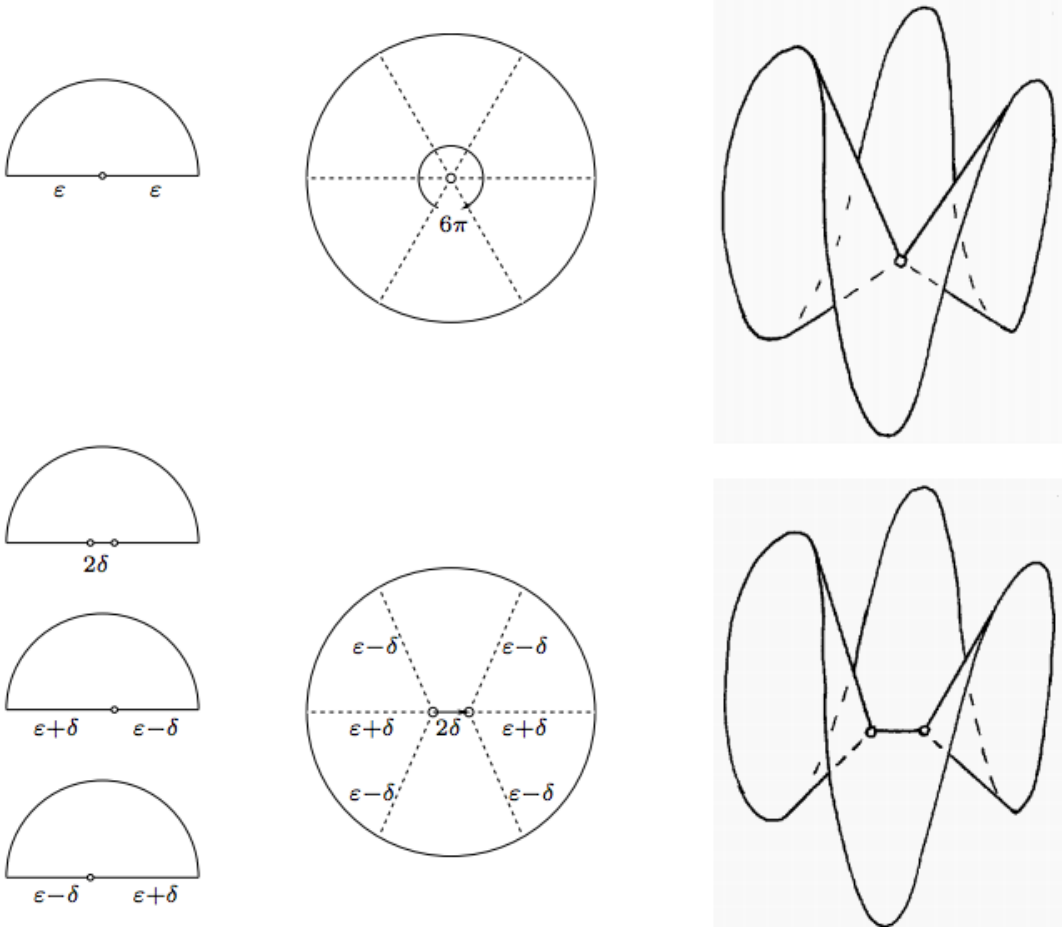

The operation of bubbling a handle allows to understand the adjacencies of strata. For example, we claim that if is a connected component of , then there exists a connected component such that we can bubble a handle on every translation surface in in order to obtain a translation surface in (compare with [44, Lemma 14]).
In fact, Lemma 20 in [44] says that contains a translation surface given by the suspension of an interval exchange transformation associated to a good standard permutation , i.e., a permutation of the form such that the permutation derived from by erasing the letters and is irreducible. Concretely, the irreducibility of means that we can use it to build (through suspension) a translation surface belonging to (in this context). See Figure 19 for an illustration of together with a “copy” of inside it.
Denote by the connected component of containing . Observe that, by definition, is obtained from by bubbling a square handle. Since the operation of bubbling a handle can be performed in a continuous way (cf. [44, Lemma 10]), we obtain the desired claim that one can bubble a (square) handle in any to obtain a translation surface in .
By exploiting this relation between and through the operation of bubbling a square handle, one can complete the proof of the proposition along the following lines (cf. Propositions 5.5 and 5.6 in [51]). Suppose that every has symplectically orthogonal Hodge-Teichmüller planes. Given , let us bubble a square handle to obtain . By degenerating the square handle (i.e., by letting the length of the sizes of the square tend to zero) in to reach , we have4949 49 Here, the fact that the angles of the torus do not degenerate (because it is always a square) is crucial. that converges to a stable nodal curve5050 50 I.e., a point in the boundary of Deligne-Mumford compactification of the moduli space of curves. of the form depicted in Figure 20.
In this process, one of the Hodge-Teichmüller planes of might be “lost” (in case it converges to the plane associated to the degenerating square handle), but at least Hodge-Teichmüller planes of will converge to (symplectically orthogonal) Hodge-Teichmüller planes of . This completes our sketch of proof of the proposition. ∎
At this point, Theorem 49 is a simple consequence of the following argument: by contradiction, suppose that is a connected component of stratum of the moduli space of translation surfaces of genus such that every has symplectically orthogonal Hodge-Teichmüller planes. By Proposition 55, there would be a connected component of such that every would also possess symplectically orthogonal Hodge-Teichmüller planes. By applying times Proposition 56, we would find a connected component of such that every would have Hodge-Teichmüller planes, a contradiction with Proposition 54.
Closing this subsection, let us give an elementary5151 51 Here, by “elementary” we mean that, instead of proving the existence of by indirect methods (including the use of Deligne-Mumford compactification), we will build directly for certain ’s. proof of the following particular5252 52 Our discussion of these particular cases follows an argument described in a blog post entitled “Hodge-Teichmüller planes and finiteness results for Teichmüller curves” in my mathematical blog [17]. cases of Theorem 49:
Proposition 57.
For each odd, there exists a translation surface in the odd connected component of the minimal stratum which does not possess symplectically orthogonal Hodge-Teichmüller planes.
Proof.
We affirm that a square-tiled surface of genus covering the square-tiled surface constructed in the proof of Proposition 54 can not have symplectically orthogonal Hodge-Teichmüller planes. In fact, if we denote by the translation covering defining the translation structure of , then where consists of all cycles projecting to zero under and is the symplectic orthogonal of . By appplying an argument similar to the proof of Proposition 53, one can check that if had symplectically orthogonal Hodge-Teichmüller planes, then two of them would be contained in and, a fortiori, would have two Hodge-Teichmüller planes, a contradiction with Proposition 54.
In view of the discussion in the previous paragraph, the proof of the proposition will be complete once we construct a degree branched cover of .
For technical reasons, it is desirable to “simplify” the geometry of before studying its covers. In this direction, let us replace by the square-tiled surface associated to the permutations , : there is no harm in doing so because belongs to the -orbit of (indeed, where and ).
Given an odd integer, let be the square-tiled surface5353 53 The “shape” of the covering was “guessed” with the help of the computer program Sage. In fact, I tried a few simple-minded finite coverings of (including for ) and I asked Sage to determine their connected components. Then, once we got the “correct” connected components (in minimal strata), I looked at the permutations corresponding to these square-tiled surfaces and I found the “partner” leading to the expressions for the permutations and . associated to the pair of permutations
By definition, is a degree cover of belonging to the stratum . Therefore, it remains only to verify that in order to complete the proof of the proposition.
Since is not hyperelliptic, we have that if and only if , where the parity of the spin structure of is defined as follows (see [44] for more details). Let (where ) be a canonical symplectic basis of . Then,
where satisfies the following properties:
- —
whenever is a simple smooth closed curve in not passing through singular points whose Gauss map has degree ;
- —
is a quadratic form representing the intersection form in the sense that .
In other words, we need to build a canonical symplectic basis of in order to compute . For this sake, we begin by fixing a basis of . We think of it as horizontal cylinders determined by the permutation whose top and bottom boundaries are glued accordingly to the permutation . Using this geometrical representation, we define the following cycles in (see Figure 22).
- —
for each , let , , and be the homology classes of the vertical cycles within the horizontal cylinders connecting the middle of the bottom side of the squares , , and (resp.) to the top side of the squares , , and (resp.);
- —
for each , , let be the homology classes of the vertical cycles within the horizontal cylinders connecting the middles of the bottom side of the square to the top side of the squares ;
- —
let be the homology class of the concatenation of the vertical cycles within the horizontal cylinders connecting the middles of the bottom side of the square to the top side of the square for , the bottom side of the square to the left side of the square , and the right side of the square to the top side of the square ;
- —
is the horizontal cycle connecting the left vertical side of the square to the right vertical side of the square , and, for , , is the horizontal cycle connecting the left vertical side of the square to the right vertical side of the square .
It is not hard to check that these cycles form a basis of . From this basis, we can produce a canonical basis of homology cycles of using the orthogonalization procedure5454 54 A Gram-Schmidt orthogonalization process to produce canonical basis of homology modulo . described in [72, Appendix C]. More precisely, we start with the cycles and . Then, by induction, we use the cycles , to successively render the cycles
into a canonical basis (where ).
Using these cycles, we are ready to compute inductively. More concretely, we affirm that for each odd. Indeed, we note that the cycles
of do not intersect the other cycles of defined above except for , and, moreover, they have trivial intersection with the cycle
satisfying . Thus, by replacing by and by applying the orthogonalization procedure to these two sets of and cycles in an independent way, we deduce that differs from by a term of the form
where , is an orthogonalization of the cycles
On the other hand, by a direct computation, one can check that
- —
, ,
- —
, ,
- —
, ,
- —
, ,
- —
,
is an orthogonalization of the cycles
Moreover, for , and for . Hence,
as it was claimed. Therefore, . ∎
5. Simplicity of Lyapunov exponents of arithmetic Teichmüller curves
The circle of ideas developed for the study of Lyapunov exponents of the Kontsevich-Zorich cocycle over the -action on moduli spaces of translation surfaces was fruitfully used in many contexts:
- —
- —
Avila and Forni [2] used the positivity of the second largest Lyapunov exponent of the KZ cocycle with respect to Masur-Veech measures to establish the weak mixing property for typical interval exchange transformations (not of rotation type) and translation flows (on higher genus surfaces);
- —
Delecroix, Hubert and Lelièvre [14] exploited the precise values of the Lyapunov exponents of the KZ cocycle over a certain closed -invariant locus of translation surfaces of genus five to confirm a conjecture of Hardy and Weber on the abnormal rate of diffusion of typical trajectories in -periodic Ehrenfest wind-tree models of Lorenz gases;
- —
Kappes and Möller [42] employed some invariants (inspired of the Lyapunov exponents of the KZ cocycle) the exact number (nine) of commensurability classes of the non-arithmetic lattices of constructed by Deligne and Mostow.
5.1. Kontsevich-Zorich conjecture and Veech’s question
In some applications of the Lyapunov exponents of the KZ cocycles, it is important to know whether they have a qualitative property called simplicity, that is, if all of them appear with multiplicity one. For instance, the most complete picture for the deviations of ergodic averages of typical interval exchange transformations and translation flows depends on the simplicity of the Lyapunov exponents of the KZ cocycle with respect to Masur-Veech measures (see [70] and [28]).
In the case of Masur-Veech measures, the simplicity of the Lyapunov exponents of the KZ cocycle was conjectured by Kontsevich and Zorich after several numerical experiments. This conjecture was fully confirmed in a celebrated work of Avila and Viana [6] after an important partial result of Forni [28].
In the case of other -invariant probability measures on moduli spaces of translation surfaces, Veech asked5555 55 Veech knew that the analog of his question for arbitrary Teichmüller flow invariant probability measures was false: for example, theKZ cocycle might have zero Lyapunov exponents along certain periodic orbits of the Teichmüller flow in (see [31, Appendix B]). if the Lyapunov exponents of the KZ cocycle are always non-zero and/or simple. This question was negatively answered by Forni and the author with two examples called Eierlegende Wollmilchsau and Ornithorynque (see, e.g., [31]): loosely speaking, these are examples of arithmetic Teichmüller curves such that the KZ cocycle over them has many zero Lyapunov exponents.
Of course, this answer to Veech’s question motivates the problem of finding criteria for the simplicity of the Lyapunov exponents of the KZ cocycle with respect to -invariant probability measures in moduli spaces of translation surfaces.
In the remainder of this section, we shall offer an answer to this problem in the context of the KZ cocycle over Teichmüller curves.
5.2. Lyapunov exponents of Teichmüller curves and random products of matrices
In this subsection, we will show that the Lyapunov exponents of the KZ cocycle with respect to -invariant probability measures supported on Teichmüller curves can be computed via random products of matrices. The relevance of this fact for our purposes is explained by the vast literature (cf. Furstenberg [34], Guivarc’h-Raugi [37], [38], Goldsheid-Margulis [36], Avila-Viana [6], etc.) on the simplicity of Lyapunov exponents of random products of matrices.
Remark 58.
The analog of this statement for Masur-Veech measures is discussed in Avila-Viana paper [6] in their reduction of the Kontsevich-Zorich conjecture to the study of “random” products of matrices in Rauzy-Veech monoids.
More concretely, let be a translation surface whose -orbit is closed in the moduli space of translation surfaces. Recall that, by a result of Smillie (see, e.g., [62]), is closed if and only if is a Veech surface, i.e., the stabilizer of is a lattice of .
We have a short exact sequence where is the group of automorphisms of and is the group of affine homeomorphisms of .
For the sake of exposition, we will assume that the group of automorphisms of is trivial: . In this case, the groups and are isomorphic.
Since the KZ cocycle over the Teichmüller flow is the quotient of the trivial cocycle
by the diagonal action of the mapping class group and the stabilizer of in the mapping class group is precisely , we have that the KZ cocycle is given by the actions on homology of the elements of appearing5656 56 I.e., the elements used to bring close to . along the orbits of .
In this setting, Eskin and the author [21] proved that the Lyapunov exponents of the KZ cocycle are seen by random products of the matrices of actions on homology of affine homeomorphisms:
Theorem 59.
Let be a Veech surface of genus . Denote by
the Lyapunov exponents of the KZ cocycle with respect to the unique -invariant probability measure on .
Then, there exists a probability measure on (the countable group) assigning non-zero mass to every element and a constant such that the Lyapunov exponents of random products of matrices in with respect to the law where is the representation induced by the action of affine homeomorphisms on are precisely
Proof.
Before discussing Lyapunov exponents, we need to “replace” the typical orbits of the geodesic flow on the hyperbolic plane by certain random walks in .
In general, the random walk on with a law of full support on is tracked by a geodesic ray in up to a sublinear error: for some and for -almost all sequences , there exists a unit-speed geodesic ray such that
as . Indeed, this is a direct consequence of Oseledets theorem saying that the random product in is “close” to the matrix , where is the top Lyapunov exponent associated to and is an angle depending on . See, e.g., Lemma 4.1 of [12] for more details.
The distribution of the angles depend on . In particular, it is far from obvious that one can choose in such a way that a typical geodesic rays in are tracked by random walks with law up to sublinear error: in concrete terms, this basically amounts to choose so that the distribution of angles is given by the Lebesgue measure.
Fortunately, a profound theorem of Furstenberg [35] ensures the existence of a probability measure on the lattice with full support and the desired (Lebesgue) distribution of angles5757 57 Actually, Furstenberg proves that the so-called Poisson boundary of is .
Once we know that a typical orbit of the geodesic flow is tracked by a random walk with sublinear error, let us come back to the discussion of Lyapunov exponents. Consider a typical geodesic ray tracked by a random walk with sublinear error.
Forni [28, §2] proved that the following general growth estimate for the KZ cocycle:
for all translation surface , where denotes the Hodge norm. From this estimate, we deduce:
Hence,
for any vector . By definition of Lyapunov exponents, this equality means that
where , resp. , is the Lyapunov exponent of with respect to random products of matrices in with law , resp. KZ cocycle . This proves the theorem. ∎
This theorem together with Avila-Viana criterion [6] for the simplicity of Lyapunov exponents of random products of matrices yield the following statement (cf. [21, Theorem 1]):
Corollary 60.
Let be a Veech surface of genus . Suppose that contains two elements and whose actions on the annihilator of the tautological plane
are given by two matrices and (in ) such that:
- (i)
is pinching, i.e., all eigenvalues of are real, simple and their moduli are distinct;
- (ii)
is twisting with respect to , i.e., for any , any isotropic -invariant -plane and any coisotropic -invariant -plane , we have .
Then, the Lyapunov exponents of the KZ cocycle with respect to the Lebesgue measure on are simple, i.e., the Lyapunov spectrum has the form
Proof.
By Theorem 59, our task is equivalent to establish the simplicity of the Lyapunov spectra of the random products with law of matrices in , where is the natural representation.
By the simplicity criterion5858 58 See also Theorem 2.17 in [50]. of Avila-Viana [6], a random product with law of matrices in has simple Lyapunov spectrum whenever the support of contains pinching and twisting matrices (in the sense of items (i) and (ii) above).
Since gives positive mass to and (because assigns positive masses to and ), the proof of the corollary is complete. ∎
Remark 61.
Theorem 59, Corollary 60 and its variants were applied by Eskin and the author to study the Lyapunov spectra of certain Teichmüller curves in genus four (of Prym type) and certain variations of Hodge structures of weight three associated to families of Calabi-Yau threefolds (including mirror quintics). See Sections 3 and 4 of [21] for more explanations.
5.3. Galois-theoretical criterion for simplicity of exponents of origamis
From the practical point of view, Corollary 60 is not quite easy to apply. Indeed, the verification of the pinching and twisting properties might be tricky: for example, Avila-Viana [6] performed a somewhat long inductive procedure in order to establish the pinching and twisting properties in their context (of Rauzy-Veech monoids).
As it turns out, Möller, Yoccoz and the author [50] found an effective version of Corollary 60 in the case of square-tiled surfaces thanks to some combinatorial arguments involving Galois theory.
In the sequel, we will state and prove a Galois-theoretical simplicity criteria and we will discuss its applications to square-tiled surfaces of genus three.
5.3.1. Galois-pinching matrices
Let be a symplectic matrix. The characteristic polynomial of is a monic reciprocal polynomial of degree . Denote by the set of roots of and let where .
We say that a matrix is Galois-pinching if its characteristic polynomial is irreducible over , its eigenvalues are real (), and the Galois group of is the largest possible, i.e., acts by the full permutation group on and the subgroup fixing pointwise acts by independent transpositions of each of the pairs .
For each , let us choose an eigenvector of associated to with coordinates in the field in such a way that for all .
The nomenclature “Galois-pinching” is justified by the following proposition:
Proposition 62.
A Galois-pinching matrix is pinching.
Proof.
By definition, all eigenvalues of a Galois-pinching matrix are real and simple. Hence, our task is to show these eigenvalues have distinct moduli.
Suppose that and are eigenvalues of . An element of the Galois group fixing must also fix , a contradiction with the fact that is the largest possible. ∎
An important point about Galois-pinching matrices is the fact that they can be detected in an effective way.
In order to illustrate this, let us consider the prototype of characteristic polynomial of a matrix in , i.e., is a monic reciprocal integral polynomial of degree four.
The following elementary proposition characterizes the polynomials with real, simple and positive roots (and, a fortiori, of distinct moduli).
Proposition 63.
The polynomial has real, simple and positive roots if and only if
Proof.
A simple calculation shows that is a root of if and only if is a root of the quadratic polynomial
of discriminant .
Since the roots of are real, simple and positive if and only if the roots of have the same properties, the desired proposition follows. ∎
The next two propositions provide a criterion for the irreducibility of over .
Proposition 64.
The polynomial is a product of two reciprocal quadratic rational polynomials if and only if .
Proof.
The quadratic polynomial with roots related to the roots of via the formula is reducible over if and only if . ∎
Proposition 65.
Let be a monic reciprocal integral polynomial of degree four. Suppose that is not a square (i.e., ) and is reducible over . Then,
is a square, i.e., .
Proof.
Since is not a square, has no rational root. Because is reducible over (by assumption), the previous proposition implies that where are monic irreducible quadratic polynomials which are not reciprocal. Thus, we can relabel the roots of in such a way that
Note that implies that and, a fortiori, . Therefore,
It follows that is a square. ∎
Furthermore, it is not hard to decide whether an irreducible monic reciprocal integral polynomial of degree four has the largest possible Galois group:
Proposition 66.
Let be irreducible over . The Galois group of is the largest possible (i.e., has order eight) if and only if
(where and ).
Moreover, in this case we have that the splitting field of contains exactly three quadratic subfields, namely, , , .
Proof.
The solution of this elementary exercise in Galois theory is explained in Lemmas 6.12 and 6.13 of [50]. For the sake of completeness, let us sketch the proof of this proposition.
Since is irreducible, acts transitively on the roots of . Thus, if can permute and independently for , then has order eight and, a fortiori, is the largest possible.
This reduces our task to show that if can not permute and independently for , then either or is an integer.
For this sake, we observe that if if doesn’t permute and independently for , then permutes simultaneously and . In this case, there are two possibilities:
- (a)
either is generated by the permutations and ,
- (b)
or is generated by the four cycle .
These cases can be distinguished as follows. The expression is invariant in case (a) (i.e., is a Klein group) but not in case (b) (i.e., is a cyclic group). Similarly, the expression is invariant in case (b) but not in case (a). Therefore:
- —
(a) occurs if and only if ;
- —
(b) occurs if and only if .
Since and , we conclude that
- —
(a) occurs if and only if ;
- —
(b) occurs if and only if .
In any case, we show that either or is an integer when can not permute and independently for . This completes our sketch of proof. ∎
In summary, the previous four propositions allow us to test whether a matrix is Galois-pinching by studying three discriminants , and naturally attached to its characteristic polynomial.
5.3.2. Twisting with respect to Galois-pinching matrices I: statements of results
After discussing the Galois-pinching property, let us study the twisting property with respect to Galois-pinching matrices. Our main result in this direction is:
Theorem 67.
Let be a Galois-pinching matrix. Suppose that has the property that and share no common proper invariant subspace. Then, there exists and, for any , there are integers , , such that the product
is twisting with respect to , i.e., for all , for any -invariant isotropic subspace of dimension and for any -invariant coisotropic subspace of dimension , we have .
This theorem constitutes the main ingredient in the simplicity criteria in [50]. Before starting its somewhat long proof, let us make some comments on its statement and applicability.
First, we observe that Theorem 67 becomes false if is replaced by in the hypothesis “ and share no common proper invariant subspace”: for example, is Galois-pinching, has no invariant subspaces, but is never twisting with respect to (because permutes the eigenspaces of ).5959 59 Logically, there is no contradiction to Theorem 67 here: and don’t fit the assumptions of this theorem since and share two common proper invariant subspaces, namely, the eigenspaces of .
Second, the condition “ and have no common proper invariant subspace” might not be easy to check in general. For this reason, the following two propositions (cf. Proposition 4.7, Lemma 5.1 and Lemma 5.5 in [50]) are useful in certain applications of Theorem 67.
Proposition 68.
Let be a Galois-pinching matrix. Suppose that is unipotent and . If and share a common proper invariant subspace, then is a Lagrangian subspace of .
Proof.
We begin by noticing that our assumptions imply that any subspace which is invariant under for some is also invariant under . Indeed, if we write and , then the binomial formula says that is nilpotent whenever is nilpotent. Hence, can be calculated by truncating the binomial series6060 60 I.e., since is nilpotent, the formal binomial series (where and ) can be interpreted as a polynomial function of . and, therefore, is a polynomial function of . In particular, any subspace invariant under is also invariant under .
In particular, our assumption that and share a common proper invariant subspace imply (in our current setting) that and share a common proper invariant subspace.
Since is Galois-pinching, any -invariant subspace is spanned by eigenvectors. Denote by the characteristic polynomial of , let and, for each , take an eigenvector of with eigenvalue whose coordinates belong to in such a way that for all in the Galois group of .
Next, let us fix a proper subset of minimal cardinality such that the subspace spanned by the vectors is -invariant. Because has integral entries, for all the subspaces are also -invariant. Thus, the minimality of the cardinality of implies that, for each , either or . This property together with the fact that is the largest possible is a severe constraint on the proper subset :
- —
either has cardinality one,
- —
or has the form
The first possibility does not occur in our context: if , then (because is unipotent); hence, using the action of , we would deduce that fixes all eigenvectors of , so that , a contradiction.
Therefore, preserves some subspace of the form . Using again the action of , we deduce that preserves all subspaces , , and the restrictions of to such planes are Galois-conjugates. As is unipotent, is an one-dimensional subspace of for all . Since the planes are mutually symplectically orthogonal, it follows that is a Lagrangian subspace. ∎
Proposition 69.
Let be a Galois-pinching matrix. Suppose that has minimal polynomial of degree with no irreducible factor of even degree and a splitting field disjoint from the splitting field of the characteristic polynomial of . Then, and do not share a common proper invariant subspace.
Proof.
We affirm that a -invariant subspace is also -invariant. In fact, and have the same characteristic subspaces because and can’t be both eigenvalues of (thanks to our assumption that the minimal polynomial of has no irreducible factor of even degree). Since an invariant subspace is the sum of its intersections with characteristic subspaces, it suffices to check that a -invariant subspace contained in a characteristic subspace of is also -invariant. Since is unipotent up to scalar factors in its characteristic subspaces, the desired fact follows from the argument used in the beginning of the proof of Proposition 68.
Let us now assume by contradiction that and share a common proper invariant subspace. From the discussion of the previous paragraph, this means that and share a common proper invariant subspace. By repeating the analysis in the proof of Proposition 68, we have that all planes , , are invariant under and .
Observe that is defined over and the trace and determinant of . From our hypothesis of disjointness of the splitting fields of and , the trace and determinant of are rational. Thus, the minimal polynomial of has degree , a contradiction with our hypotheses. ∎
After these comments on the statement of Theorem 67, let us now prove this result.
5.3.3. Twisting with respect to Galois-pinching matrices II: proof of Theorem 67
Consider the Galois-pinching matrix and denote by the set of its eigenvalues. For each , we select eigenvectors of associated to with coordinates in the field behaving coherently with respect to the Galois group of the characteristic polynomial of , i.e., for all .
The twisting propertyfor a matrix with respect to can be translated in terms of combinatorial properties of certain graphs naturally attached to its exterior powers .
More concretely, for each , let be the collection of all subsets of with cardinality . Note that, for each , we can associated a multivector . By definition, the set is a basis of diagonalizing : indeed, where .
In this setting, the -invariant isotropic subspaces are easy to characterize. If and is the collection of such that is injective, then the subspace generated by is isotropic if and only if . Using this fact and an elementary (linear algebra) computation (cf. [50, Lemma 4.8]), it is not hard to check that:
Lemma 70.
A matrix is twisting with respect to if and only if for every the coefficients of the matrix in the basis satisfy the condition
| (5.1) |
In other words, if is oriented graph with set of vertices and set of arrows , then is twisting with respect to if and only if is a complete graph for each .
In general, it is not easy to apply this lemma because the verification of the completeness of might be tricky. For this reason, we introduce the following (classical) notion:
Definition 71.
The graph is mixing if there exists such that for all we can find an oriented path in of length going from to .
Remark 72.
In this definition, it is important to connect two arbitrary vertices by a path of length exactly (and not only of length ). For instance, the graph in Figure 23 is not mixing because all paths connecting to have odd length while all paths connecting to have even length.
The relevance of this notion is explained by the following proposition (saying that if is mixing, then is complete for certain products of the matrices and ).
Proposition 73.
Let us assume that the graph is mixing with respect to an integer . Then there exists a finite family of hyperplanes of such that the following holds. For any , the graph associated to the matrix
is complete for all sufficiently large .
Proof.
Let us denote . By definition,
Consider the linear forms:
Our assumption on ensures that there are coefficients such that
We want to prove that . Since is a sum of exponentials with non-vanishing coefficients, our task is to show that can be taken so that potential cancelations among these terms can be avoided.
Here, the key idea is to prove that, for , the linear forms and are distinct. Indeed, suppose that this is the case and let us define . By hypothesis, each is a hyperplane. Since there are only finitely many paths of length on , the collection of corresponds to a finite family of hyperplanes . Hence, if we take , then
for sufficiently large (because the coefficients are mutually distinct).
Let us now complete the proof of the proposition by showing that for . Given and , , we claim that the following coefficients of and differ:
In fact, an equality between these coefficients would imply a relation
On the other hand, if then (since ). So, if we take and with and otherwise, then
Thus, or , a contradiction in any case (because Galois-pinching implies that ). ∎
This proposition suggests the following strategy of proof of Theorem 67:
- —
Step 0: Show that the graphs are always non-trivial, i.e., there is at least one arrow starting at each of its vertices.
- —
- —
Let us now consider the cases of Theorem 67. Unfortunately, there is no “unified” argument to deal with all cases and we are obliged to separate the case from .
- —
Step 2: In the case , we will show that (with as in Step 1) is mixing for all . By Proposition 73, there is a product of powers of and such that is complete for all . Using this information, we will prove that is mixing. By Proposition 73, a certain product of powers of and is twisting with respect to , so that this completes the argument in this case.
- —
Step 3: In the special case , we will show that either or a closely related graph is mixing and we will see that this is sufficient to construct such that is complete.
During the implementation of this strategy, the following easy remarks will be repeatedly used:
Remark 74.
If , then is invariant under the action of Galois group on the set (parametrizing all possible arrows of ). In particular, since the Galois group is the largest possible, whenever an arrow belongs to , the inverse arrow also belongs to . Consequently, always contains loop of even length.
Remark 75.
A connected graph is not mixing if and only if there exists an integer such that the lengths of all of its loops are multiples of .
The next lemma deals with Step 0 of the strategy of proof of Theorem 67:
Lemma 76.
Let . Then, each is the start of at least one arrow of .
Remark 77.
The symplecticity of is really used in this lemma: the analogous statement for general invertible (i.e., ) matrices is false.
Proof.
Every -dimensional subspace is isotropic. Hence, and the lemma follows in the case from the invertibility of .
So, we can assume that . The invertibility of ensures that, for each , there exists with . If , we are done. If , i.e., , our task is to “convert” into some with . For this sake, it suffices to prove that if and , then there exists with and .
Keeping this goal in mind, note that if , then we can write with . Also, if and only if the minor of associated to and is invertible.
Hence, we can choose bases to convert invertible minors of into the identity matrix: if , then we can find such that and
Denote by the symplectic form. Observe that because and belong to the span (an isotropic subspace as ). Thus, the simplecticity of implies that
Since (as ), it follows that and for some .
This allows us to define . Note that and the minor of associated to and is obtained from the minor by replacing the line associated to with the line associated to . In the basis , the minor differs from the identity minor precisely by the replacement of the line associated to by the line associated to , that is, one of the entries of was replaced by the coefficient . Thus, the determinant of the the minor is
Therefore, has the desired properties. This completes the proof of the lemma. ∎
Let us now discuss Step 1 in the strategy of proof of Theorem 67.
Lemma 78.
Let be a Galois-pinching matrix. Suppose that has the property that and share no common proper invariant subspace. Then, is mixing.
Proof.
In the sequel, our figures are drawn with the convention that two points inside the same ellipse represent a pair of eigenvalues of of the form , .
For , the set consists of exactly one pair . Hence, all possible Galois invariant graphs are described in Figure 24.
In the first situation, by definition, we have that (and ). Thus, and share a common invariant subspace, a contradiction with our assumptions.
In the second situation, by definition, we have that and . So, and thus and share a common invariant subspace, a contradiction with our standing hypothesis.
In the third situation, we have that the graph is complete, and, a fortiori, mixing.
This establishes the case of the lemma. After this “warm up”, let us investigate the general case .
First, let us assume that all arrows in have the form . Then, , and, since6161 61 Of course, this arguments breaks up for and this is why we had a separate argument for this case. , the subspace is non-trivial. Thus, in this case, and share a common non-trivial subspace, a contradiction with our assumptions.
Therefore, we can assume (without loss of generality) that contains an arrow with . By Remarks 74 and 75, this implies that all arrows of this type belong to and, moreover, is mixing whenever it contains a loop of odd length. Hence, our task is reduced to exhibit loops of odd length in .
It is not hard to construct a loop of length in when : indeed, this follows immediately from the presence of all arrows with in (cf. Figure 25).
On the other hand, for , we need a different argument. If were the non-mixing graph Galois-invariant depicted in Figure 26, we would have and . So, and would share a common invariant subspace, a contradiction with our hypothesis.
Thus, must contain the graph of Figure 26 and an extra arrow. In this situation, it is not hard to build up loops of lenght .
In any case, we proved that, under our assumptions, contains a loop of length whenever . This completes the proof of the lemma. ∎
We are now ready to implement Step 2 of the strategy of proof of Theorem 67. The first part of this step is implemented by the following lemma:
Lemma 79.
Let be a Galois-pinching matrix. Suppose that and is a matrix such that is complete. Then, is mixing for all .
Proof.
Since is invariant under the Galois group (see Remark 74), it consists of a certain number of orbits of the action of on .
As it turns out, it is not hard to check that all -orbits on have the form
where and . In particular, the -orbits on are naturally parametrized by the set
It follows that for some , where is the graph whose vertices are and whose arrows are
We affirm that is not mixing if and only if
- —
either and ,
- —
or and .
Indeed, suppose that for or for . Then, since , one can show that is not mixing simply because it is not connected! For the reciprocal statement, one proceeds as follows (cf. [50, Proposition 4.19] for more details): first, one converts pairs into a single point , so that becomes a new graph ; second, one proves that is connected whenever ; from the connectedness of one can prove that is connected; since the connectedness of allows us to construct loops of odd length, one obtains (from Remarks 74 and 75) that is mixing whenever and this concludes the argument.
Once we dispose of this characterization of the mixing property for , we can complete the proof of the lemma as follows. Suppose that is complete but is not mixing for some (where ). The discussion of the previous paragraph implies that
for some for or for . For the sake of concreteness, we shall discuss only6262 62 The particular case when is left as an exercise to the reader (see also [50]). the case . In this situation, there is an arrow of with . This means that , and hence we can find such that and
In other words, as we also did in Step 0 (cf. the proof of Lemma 76), we can use to “convert” the minor of associated to into the identity.
We claim that if , then for all . Indeed, the same arguments with minors and replacement of lines yield that if this were not true, say , then there would be an arrow from to . Since , we would have , and, thus, for some , a contradiction (proving the claim).
This claim permits to complete the proof of the lemma: in fact, it implies that is a linear combination of , , a contradiction with the completeness hypothesis on . ∎
The second part of Step 2 of the strategy of proof of Theorem 67 is the following lemma:
Lemma 80.
Let be a Galois-pinching matrix. Suppose that and is a matrix such that is complete for all . Then, is mixing.
Proof.
Recall that the -orbits on are
with and .
Hence, in the case , these orbits are parametrized by the set . For the sake of simplicity, let us denote the -orbits on by
and let us write
where .
It is possible to show6363 63 Again by the arguments with “minors” described above. that if is complete for each , then contains two consecutive integers, say and (see [50] for more details).
Thus, our task is reduced to prove that is mixing when .
In this direction, we establish first the connectedness of . For this sake, note that it suffices6464 64 The general case of two general vertices and follows by producing a series of vertices , , , with for . to connect two vertices and with . Given such and , let us select with , and let us consider obtained from by replacing the elements of by their inverses. Since , we have and . From our assumption , we infer the presence of the arrows and in . This proves the connectedness of .
Next, we show that is mixing. The Galois invariance of guarantees that it contains loops of length (see Remark 74). So, it suffices to exhibit some loop of odd length in (see Remark 75). For this sake, let us fix an arrow of . The construction “ for ” performed in the previous paragraph allows us to connect to by a path of length in . In this way, we get a loop (based on ) in of length . This proves the lemma. ∎
Finally, let us comment on Step 3 of the strategy of proof of Theorem 67, i.e, the special case of this theorem. Consider a symplectic form . Since has dimension and is non-degenerate, has dimension .
By denoting by the eigenvalues of a Galois-pinching matrix , we have the following basis of
- —
, , , ;
- —
where .
In general, given , we can use to construct a graph whose vertices are and , and whose arrows connect vertices associated to non-zero entries of .
Remark 81.
By definition, , so that is an eigenvalue of . In principle, this poses a problem to derive the analog of Proposition 73 with replaced by . But, as it turns out, the simplicity of the eigenvalue of can be exploited to rework the proof of Proposition 73 to check that if is mixing, then there are adequate products of and powers of such that is complete (cf. Proposition 4.26 in [50]).
In this setting, the third step of our strategy of proof of Theorem 67 amounts to show that:
Lemma 82.
Let be a Galois-pinching matrix. Suppose that is a matrix such that is complete. Then, either or is mixing.
Proof.
We write with . If contains two consecutive integers, then the arguments from the proof of Lemma 80 can be used to show that is mixing.
Hence, we can assume (without loss of generality) that does not contain two consecutive integers. Since (see Lemma 76, i.e., Step 0), this means that , or . As it turns out, the cases are “symmetric”, as well as the cases .
For the sake of exposition, we will deal only6565 65 The “symmetric” cases are left as an exercise for the reader. with the cases and . We will show that is impossible, while implies that is mixing.
We begin by . This means that we have an arrow with . So, we can find with and
Since , the arrows , , and do not belong . Thus, . On the other hand, because is symplectic, (with ). It follows that for all , that is, preserves the -invariant subspace . By exploiting this fact6666 66 As explained in the proof of Proposition 4.27 in [50]., one reaches a contradiction with our assumption of completeness of . Thus, is impossible.
Suppose now that and let us show that is mixing. For this sake, we claim that, in this situation, it suffices to construct arrows from the vertex to and6767 67 Notice that the action of the Galois group can not be used to revert arrows of involving the vertex , so that the two previous statements are independent. vice-versa. Assuming the claim, we can use the Galois action to see that once contains some arrows from and some arrows to , it contains all such arrows. In other words, if the claim is true, we have the situation depicted in Figure 27.
Thus, we have loops of length (in ), and also loops of length (based on ), so that is mixing (cf. Remark 75). Hence, it remains only to show the claim.
The existence of arrows from to follows from the same kind of arguments involving “minors” above (i.e., selecting as above, etc.) and we will not repeat it here.
Instead, we focus on showing that there are arrows from to . The proof is by contradiction: otherwise, one would have .
We want to use this information to determine the image of under . Here, the following elementary (linear algebra) fact is useful. Given is a symplectic -plane on equipped with the standard symplectic form , let where is a basis of and is a basis of the symplectic orthogonal such that . Then, is well-defined (independently on the choices) and is collinear to if and only if or . (See, e.g., [50, Proposition 4.28] for a proof of this fact.)
Since , the fact stated above says that if , then
Once again, an argument using “minors” says that this is a contradiction with our assumption that is complete. This completes the proof of the lemma. ∎
At this point, the proof of Theorem 67 is complete (compare with Steps 0, 1, 2 and 3 of the strategy of proof outlined above). Indeed, the case follows from Lemma 78 and Proposition 73. The generic case follows from Lemmas 78, 79, 80 and Proposition 73. Finally, the special case follows from Lemmas 78, 82, Proposition 73 and Remark 81.
5.3.4. Two simplicity criteria for the Lyapunov exponents of origamis
We are now in position to discuss the simplicity of Lyapunov exponents of square-tiled surfaces.
Let be a reduced6868 68 This means that the group of relative periods of is . square-tiled surface of genus with a trivial group of automorphisms. In this case, the group of affine homeomorphisms of is naturally isomorphic to a finite-index subgroup of , namely, the Veech group of (i.e., the stabilizer of in ).
The action of on respects the decomposition
where is the annihilator of and is the symplectic orthogonal of . Note that this decomposition is defined over (because is a square-tiled surface) and, hence, the elements of act on via symplectic matrices in .
Our discussion of the Galois-pinching and twisting properties give the following two simplicity criteria for the Lyapunov exponents of square-tiled surfaces (cf. Theorems 1.1 and 5.4 in [50]).
Theorem 83.
Let be a reduced square-tiled surface of genus with trivial group of automorphisms. Suppose that and are affine homeomorphisms of whose actions on are given by matrices and in such that:
- —
is Galois-pinching, and
- —
is unipotent and is not a Lagrangian subspace.
Then, the Lyapunov exponents of the KZ cocycle with respect to the unique -invariant probability measure support on are simple.
Proof.
Theorem 84.
Let be a reduced square-tiled surface of genus with trivial group of automorphisms. Suppose that and are affine homeomorphisms of whose actions on are given by matrices and in such that:
- —
is Galois-pinching, and
- —
the minimal polynomial of has degree with no irreducible factor of even degree and a splitting field disjoint from the splitting field of the characteristic polynomial of .
Then, the Lyapunov exponents of the KZ cocycle with respect to the unique -invariant probability measure support on are simple.
From the practical point of view, it is sometimes more convenient to apply the following corollary of Theorem 83.
Corollary 85.
Let be a reduced square-tiled surface of genus with trivial group of automorphisms. Suppose that acts on by a Galois-pinching matrix in and there exists a rational direction such that decomposes into a finite union of cylinders whose waist curves generate a subspace of of dimension .
Then, the Lyapunov exponents of the KZ cocycle with respect to the unique -invariant probability measure support on are simple.
Proof.
In view of Theorem 83, it suffices to construct acting on by an unipotent matrix such that is not Lagrangian.
We may assume that decomposes into a collection of horizontal cylinders whose waist curves generate an isotropic subspace of of dimension . Note that the image of under is one-dimensiona (because is isotropic), so that
Let be an integer such that and the affine homeomorphism with linear part fixes all horizontal separatrices at all points of the set of conical singularities of .
We affirm that is the desired affine homeomorphism. Indeed, for each horizontal cylinder of , let us fix a relative cycle crossing upwards. By definition, the matrix of the action of on satisfies
for some . Since fixes each , we have that is a nilpotent operator of degree two on . The image of under is contained in , so that
In particular, is not Lagrangian.
It remains only to prove that . For this sake, consider the oriented graph whose vertices are the connected components of and whose edges , , go from the component of containing the bottom boundary of to the component of containing the top boundary of .
Note that, for each vertex of , we have the relation
because these are the homology classes of the two components of a small neighborhood of in .
The orbit of the vertical flow on through a generic point of provides a way to construct a simple oriented loop in containing the edge .
On the other hand, contains two distinct simple oriented loops at least: otherwise, would consist of a single loop, so that the previous relations would say that all classes are equal, a contradiction with our assumption that the span of the classes has dimension .
Let us fix two distinct simple oriented loops and in . By definition, there is an edge of not contained in for . Consider a loop on obtained by concatenation of with and some horizontal saddle connections. Observe that
because fixes horizontal saddle connections.
Denote by the homological intersection between and . By definition,
Since for all and we can find edges in not contained in for , we get that
Thus, intersects non-trivially some for all .
In particular, if we choose and such that , then we obtain a cycle whose image under is not zero6969 69 Because intersects some in a non-trivial way.. Hence, .
This completes the proof of the corollary. ∎
The simplicity criteria in Corollary 85 was originally applied in our joint paper [50] with Möller and Yoccoz to study the Lyapunov exponents of square-tiled surfaces in the minimal stratum of the moduli space of translation surfaces of genus .
More precisely, we exhibited many infinite families of square-tiled surfaces in both connected components of fitting the assumptions of Corollary 85 (cf. Theorem 1.3 in [50]), and, conditionally on a conjecture of Delecroix and Lelièvre on the classification of -orbits of square-tiled surfaces in , we showed that all but finitely many square-tiled surfaces in have simple Lyapunov spectrum.
In a nutshell, the idea of the proof of these facts goes as follows. Given a family , , of square-tiled surfaces and a family of affine homeomorphisms , let be the matrices of and denote by the characteristic polynomial of . In our paper [50], we identify several7070 70 If the conjecture of Delecroix-Lelièvre is true, then the families described in [50] include all but finitely many -orbits of square-tiled surfaces in . such families with the property that is irreducible and the discriminants , and introduced in Proposition 66 are polynomial functions of high “reduced” degree of the parameter . By Siegel’s theorem (on integral points in algebraic curves of positive genus), we have that the discriminants , and are not squares for all sufficiently large, i.e., for all where is an effective (but doubly exponential) function of the coefficients of , and . By Proposition 66, it follows that is Galois-pinching for all . Since these families are built in such a way that the cylinders in some rational direction span a subspace of dimension two in homology, we can conclude thanks to Corollary 85.
Remark 86.
After the publication of [50], Bonatti, Eskin and Wilkinson announced an unconditional proof of the simplicity of the Lyapunov exponents of all but finitely many square-tiled surfaces in . Their arguments are based on the continuity of the Lyapunov spectra of -invariant probability measures in moduli spaces of translation surfaces (and, for this reason, the conclusions of Bonatti, Eskin and Wilkinson are not effective in the sense explained above).
5.4. A counterexample to an informal conjecture of Forni
In his paper [30], Forni obtained a geometrical criterion for the non-uniform hyperbolicity of the KZ cocycle with respect to a given -invariant probability measure on the moduli space of translation surfaces. In particular, Forni showed that if the support of contains a translation surface decomposing completely into parallel cylinders whose waist curves generate a Lagrangian subspace of , then all Lyapunov exponents of the KZ cocycle with respect to are non-zero.
During some informal conversations with the author, Forni conjectured that the converse statement to his theorem could be true: if the Lyapunov exponents of the KZ cocycle with respect to are all non-zero, then the support of contains a translation surface completely decomposing into parallel cylinders whose waist curves generate a Lagrangian subspace in homology.
In our joint work [15] with Delecroix, we found two counterexamples to this informal conjecture. For the sake of exposition, we present only one of them.
Theorem 87.
The -orbit of the square-tiled surface of genus associated to the pair of permutations and supports an unique -invariant probability measure such that all Lyapunov exponents of the KZ cocycle with respect to are non-zero but the subspaces generated by complete decompositions in parallel cylinders of surfaces in are never Lagrangian.
Proof.
An elementary calculation shows that -orbit of has exactly three square-tiled surfaces , and (cf. Proposition 2.3 of [15]). A direct inspection of these square-tiled surfaces reveals that the subspace generated by the waists curves of the horizontal cylinders of has dimension for all (cf. Proposition 1.2 of [15]). In particular, this means that the subspaces generated by complete decompositions in parallel cylinders of surfaces in are never Lagrangian (because has genus ).
Therefore, the proof of the theorem will be complete once we show that the Lyapunov exponents of the KZ cocycle with respect to are all non-zero. In this direction, we will actually use Corollary 85 to prove a stronger property, namely, the simplicity of these Lyapunov exponents. More concretely, the discussion of the previous paragraph (about the subspaces generated by waist curves of cylinders) says that we can apply Corollary 85 once we exhibit an affine homeomorphism acting on through a Galois-pinching matrix. Fortunately, this goal is not hard to accomplish: first, one shows that the affine homeomorphisms and of with linear parts and act on (equipped with a certain basis) via the matrices
(cf. Lemma 2.4 in [15]). A straightforward computation reveals that the affine homeomorphism acts on via a matrix with characteristic polynomial
In particular, is Galois-pinching: indeed, this is a consequence of Proposition 66 because is an irreducible polynomial such that the discriminants
and are not perfect squares.
This proves the desired theorem. ∎
6. An example of quaternionic Kontsevich-Zorich monodromy group
The features of the -action on the moduli spaces of translation surfaces (and its applications to the study of interval exchange transformations, translation flows and billiards) are intimately related to the properties of the so-called Kontsevich-Zorich (KZ) cocycle.
In particular, it is not surprising that the KZ cocycle is one of the main actors in the recent groundbreaking work of Eskin and Mirzakhani [22] towards the classification of -invariant measures on moduli spaces of translation surfaces.
Partly motivated by this scenario, some authors decided to investigate the possible monodromies of the KZ cocycle, i.e., the potential Zariski closures of the corresponding groups of matrices.
6.1. Filip’s classification of Kontsevich-Zorich monodromy groups
By extending a previous work of Möller [57] on the KZ cocycle over Teichmüller curves, Filip [25] showed that a version of the so-called Deligne’s semisimplicity theorem holds for the KZ cocycle in general.
In plain terms, this means that the KZ cocycle can be completely decomposed into -irreducible pieces, and, furthermore, each piece respects the Hodge structure coming from the Hodge bundle. Equivalently, the Kontsevich-Zorich cocycle is always diagonalizable by blocks and its restriction to each block is related to a variation of Hodge structures of weight .
The previous paragraph seems abstract at first sight, but, as it turns out, it gives geometrical constraints on the possible groups of matrices obtained from the KZ cocycle.
More precisely, by exploiting the known tables7171 71 See [26, §3.2]. for monodromy representations coming from variations of Hodge structures of weight over quasiprojective varieties, Filip [26] classified (up to compact and finite-index factors) the possible Zariski closures of the groups of matrices associated to restrictions of the KZ cocycle to an irreducible piece. In particular, there are at most five types of possible Zariski closures for blocks of the KZ cocycle (cf. Theorems 1.1 and 1.2 in [26]):
- (i)
the symplectic group in its standard representation;
- (ii)
the (generalized) unitary group in its standard representation;
- (iii)
in an exterior power representation;
- (iv)
the quaternionic orthogonal group (sometimes called , or ) of matrices on respecting a quaternionic structure and an Hermitian (complex) form of signature in its standard representation7272 72 In concrete terms, is the group of matrices with coefficients in the quaternions H such that where is the transpose of and is a reversion on H.;
- (v)
the indefinite orthogonal group in a spin representation.
Moreover, it is not hard to check that each of these items can be realized as an abstract variation of Hodge structures of weight over abstract curves and/or Abelian varieties.
6.2. Realizability problem for Kontsevich-Zorich monodromy groups
It is worth to stress out that Filip’s classification of the possible blocks of the KZ cocycle comes from a general study of variations of Hodge structures of weight .
Thus, it is not clear whether all items above can actually be realized as a block of the KZ cocycle over the closure of some -orbit in the moduli spaces of translations surfaces.
In fact, it was previously known in the literature that (all groups listed in) items (i) and (ii) appear as blocks of the KZ cocycle over closures of -orbits of translation surfaces given by certain cyclic cover constructions.
On the other hand, it is not obvious that the other 3 items occur in the context of the KZ cocycle: indeed, this realizability question was explicitly posed by Filip in [26, Question 5.5] (see also §B.2 in Appendix B of Delecroix-Zorich paper [16]).
Filip, Forni and myself [27] gave a partial answer to this question by showing that the case of item (iv) is realizable as a block of the KZ cocycle:
Theorem 89.
There exists a square-tiled surface of genus 11 such that the restriction of the KZ cocycle over to a certain -irreducible piece acts through a Zariski dense subgroup of in its standard representation (modulo finite-index subgroups).
Remark 90.
Thanks to an exceptional isomorphism between the real Lie algebra in its standard representation and the second exterior power representation of the real Lie algebra , this theorem also says that the case of of item (iii) is realized.
Remark 91.
The examples constructed by Yoccoz, Zmiaikou and myself [53] of regular origamis associated to the groups of Lie type might lead to the realizability of all groups in item (iv). In fact, what prevents us to show that this is the case is the absence of a systematic method to prove that the natural candidates to blocks of the KZ cocycle over these examples are actually irreducible pieces.
Remark 92.
The realizability of some and/or all groups in items (iii) and (v) might be a delicate problem: indeed, contrary to our previous remark about the realization of all groups in item (iv), we are not aware of examples of translation surfaces which could solve this question.
The remainder of this section is dedicated to the proof of Theorem 89.
6.3. A quaternionic cover of a L-shaped orgami
The starting point of the square-tiled surface in Theorem 89 is the following observation. The group is related to quaternionic structures on vector spaces. In particular, it is natural to look for translation surfaces possessing an automorphism group admitting representations of quaternionic type.
Note that automorphism groups of translation surfaces (of genus ) are always finite7373 73 E.g., by Hurwitz’s theorem saying that a Riemann surface of genus has automorphisms at most. and the simplest finite group with representations of quaternionic type is the quaternion group
where , , and .
This indicates that we should look for translation surfaces whose group of automorphisms is isomorphic to . A concrete way of building such translation surfaces is to consider ramified covers of “simple” translation surfaces such that the group of deck transformations of is isomorphic to .
The first natural attempt is to take the flat torus, and define as the translation surface obtained as follows. We let , , be copies of the flat torus . Then, we glue by translation the rightmost vertical, resp. topmost horizontal side, of with the leftmost vertical, resp. bottommost horizontal side, of , resp. for each . In this way, we obtain a translation surface tiled by eight squares , , such that the natural projection is a ramified cover (branched only at the origin of ) whose group of automorphisms is isomorphic to (namely, an element acts by translating to for all ).
The translation surface constructed above is a well-known square-tiled surface: it is the so-called Eierlegende Wollmilchsau in the literature (see e.g. [29] and [40]).
Unfortunately, the Eierlegende Wollmilchsau is not a good example for our current purposes. Indeed, it is known that the KZ cocycle over the -orbit of the Eierlegende Wollmilchsau acts through a finite group of matrices: see, e.g., the work [52] of Yoccoz and the author. In particular, this provides no meaningful information towards realizing monodromy groups because in Filip’s list one always ignores compact and/or finite-index factors.
After this frustrated attempt, we are led to look at other translation surfaces distinct from the flat torus. In this direction, it is natural to consider the simplest L-shaped square-tiled surface in genus described in Figure 2 above.
Next, we build a ramified cover of in a similar way to the construction of the Eierlegende Wollmilchsau: we take copies , , of this L-shaped square-tiled surface, and we glue by translations the corresponding vertical, resp. horizontal, sides of and , resp. . Equivalently, we label the sides of as indicated in Figure 28
and we glue by translations the pairs of sides with the same labels.
The natural projection is a ramified cover branched only at the unique conical singularity of . Also, the automorphism group of is isomorphic to and each acts on by translating each to for all .
A direct inspection reveals that has four conical singularities (at the points labelled , , and in Figure 28) whose cone angles are . In particular, is a genus surface.
In this setting, the KZ cocycle over is simply the action on of the group of affine homeomorphisms of .
6.4. Block decomposition of the KZ cocycle over
Similarly to the so-called wind-tree models studied by Delecroix, Hubert and Lelièvre [REF], the translation surface has a rich group of symmetries allowing us to decompose the KZ cocycle into blocks.
More precisely, by taking the quotient of by the center of its automorphism group , we obtain a translation surface of genus with four conical singularities whose cone angles are . Moreover, by taking the quotient of by the subgroups , and of its automorphism group , we obtain three genus surfaces , and each having two conical singularities whose cone angles are . In summary, we have intermediate covers and for such that and .
These intermediate covers lead us towards a natural candidate for blocks of the KZ cocycle over . More concretely, a translation cover induces a decomposition
where is the symplectic orthogonal of the vector space of cycles on projecting to zero under . Thus, if we take an adequate finite-index subgroup of whose elements commute7474 74 I.e., up to finite-index, the KZ cocycle commutes with the action of on . with the automorphisms of , then we obtain that the action of can be virtually diagonalized by (symplectically orthogonal) blocks
where:
- —
is the subspace generated by and ,
- —
is induced by the cover ,
- —
is induced by the cover for each , and
- —
is the symplectic orthogonal of the direct sum of the other subspaces.
See Subsection 5.3 of [27] for more details.
These subspaces have the structure of -modules, and, by a quick comparison with the character table of , one can show that , , , and (resp.) are the isotypical components of the trivial, -kernel, -kernel, -kernel and the unique four-dimensional faithful irreducible representation of (resp.): for example, is the isotypical component of because acts as on and the sole character of to take a negative value at is precisely .
Furthermore, is -dimensional because and have genera and (so that and have dimensions and ), and is the symplectic orthogonal of the symplectic subspace . Hence, as a -module.
6.5. Some constraints on Kontsevich-Zorich monodromy group of
Note that acts via symplectic automorphisms of the -module (because the actions of and the automorphism group on commute), and carries a quaternionic structure. In particular, we are almost in position to apply Filip’s classification results to determine the group of matrices through which acts on .
Indeed, if we have that acts irreducibly on , then Filip’s list of possible monodromy groups says that acts through a (virtually Zariski dense) subgroup of (because preserves a quaternionic structure on ).
However, there is no reason for the action of the affine homeomorphisms on an isotypical component of the automorphism group to be irreducible in general (as far as we know). Nevertheless, the semi-simplicity theorems of Möller [57] and Filip [25] mentioned above tells us that can split into irreducible pieces in one of the following three ways:
- (a)
is irreducible, i.e., it does not decompose further;
- (b)
where and are irreducible pieces;
- (c)
where , , are irreducible pieces isomorphic to .
By applying Filip’s classification to each of these items, we find that (up to compact and finite-index factors) there are just three possibilities:
- (a’)
if is -irreducible, then acts through a Zariski-dense subgroup of ;
- (b’)
if with and irreducible pieces, then acts through a subgroup of ;
- (c’)
if with , , irreducible pieces isomorphic to , then acts through a subgroup of .
At this point, we reduced the proof of Theorem 89 to show that we are in situation (a’) or, equivalently, the situations (b’) and (c’) can’t occur.
In the next two subsections, we shall rule out (c’) and (b’) respectively.
6.6. Ruling out monodromy on
Suppose that acts on as described in item (c’). In this situation, the nature7575 75 A product of three copies of the compact group . of would force all Lyapunov exponents of the restriction of the KZ cocycle to to vanish. Therefore, we can rule out this situation by showing the following proposition:
Proposition 93.
Some Lyapunov exponents of KZ cocycle on are not zero.
The proof of this proposition relies crucially on the formulas of Bainbridge [7], Chen and Möller [13], and Eskin-Kontsevich-Zorich [19] for the sum of non-negative Lyapunov exponents for the square-tiled surfaces. More concretely, we can derive this proposition as follows.
First, since , Bainbridge work [7] ensures that the non-negative Lyapunov exponents associated to are and .
Secondly, since , , the work of Chen and Möller [13] says that the sum of non-negative Lyapunov exponents associated to is . Since we already know that the non-negative Lyapunov exponents of are and , we conclude that the non-negative Lyapunov exponents associated to
are with multiplicity one and with multiplicity four.
Thirdly, the fact that has quaternionic nature forces each of its Lyapunov exponent to appear with multiplicity four (at least). Since is -dimensional, the Lyapunov exponents associated to have the form
It follows that the sum of the non-negative Lyapunov exponents of is
At this point, we will prove that is not zero by using Eskin-Kontsevich-Zorich formula [19] saying that the sum of the non-negative Lyapunov exponents of a square-tiled surface of genus is given by the following expression:
where is a pair of permutations associated to .
In our case, and its contains twelve square-tiled surfaces whose flat geometries are explicitely described in [27, Subsection 5.4]. From this, we can show that
This means that , and, thus, the proof of Proposition 93 is complete.
Remark 94.
We have just proved that we are in situation (a’) or (b’). Hence, we already know that the KZ cocycle over acts on a irreducible piece through a Zariski dense subgroup of or (modulo compact and/or finite-index factors). Of course, this suffices to deduce that we can realize a non-trivial case ( or ) of item (iv) in Filip’s list, but, for the sake of completeness, we will show in the next subsection how to rule out the situation (b’).
6.7. Ruling out monodromy on
Suppose that acts on as described in item (b’), i.e., we have a -invariant decomposition with and .
In this case, the sole possibility for the subspace is to be the central subspace of any matrix of any element of acting on with ‘‘simple spectrum’’ in the quaternionic sense7676 76 I.e., the matrix has an unstable (modulus ) eigenvalue, a central (modulus ) eigenvalue, and an stable (modulus ) eigenvalue, all of them with multiplicity four.
Therefore, we can contradict the existence of by exhibiting two matrices of the action of on with “simple spectrum” whose central spaces are distinct.
Unfortunately, we do not have an abstract method to produce two matrices with the properties above (compare with Remark 91 above). Thus, we are obliged to compute by hands the action of some elements of .
In this direction, we observe that acts on via . From this, it is not hard to check that a basis of is given by the following twelve (absolute) cycles
where , , , , and , , and are the (relative) cycles in Figure 28.
Next, we consider the affine homeomorphisms with linear parts
and fixing (pointwise) the conical singularities of . Geometrically, are Dehn multitwists of along the cylinders in directions .
A straightforward calculation shows that the actions of on with respect to the basis are given by the following matrices :
and
See Subsections 6.2, 6.3 and 6.4 of [27] for more details.
From these formulas, we can exhibit two elements of acting on through matrices with “simple spectrum” and distinct central subspaces. In fact, let us fix such that and belong to : this is possible because has finite-index in . Note that these elements act on by matrices with “simple spectrum”: indeed, a computation reveals that and have characteristic polynomials
and
In particular, has three eigenvalues (each of them with multiplicity four), namely, , and , and has three eigenvalues (each of them with multiplicity four), namely, , and , so that and have “simple spectrum”.
Furthermore, it is not hard to see that the central eigenspace of (associated to the eigenvalue ) is spanned by the following four vectors:
and the central eigenspace of (associated to the eigenvalue ) is spanned by the following four vectors:
Thus, and are distinct7777 77 Actually, span a -dimensional vector space. Since , resp. , is also the central space of , resp. , this means that we are not in situation (b’), so that the proof of Theorem 89 is complete.
References
- [1] P. Apisa, Orbit Closures in Hyperelliptic Components of Strata, available at arXiv:1508.05438. Preprint (2015).
- [2] A. Avila and G. Forni, Weak mixing for interval exchange transformations and translations flows, Annals of Math. 165 (2007), 637–664.
- [3] A. Avila and S. Gouëzel, Small eigenvalues of the Laplacian for algebraic measures in moduli space, and mixing properties of the Teichmüller flow, Ann. of Math. (2) 178 (2013), 385–442.
- [4] A. Avila, S. Gouezel and J.-C. Yoccoz, Exponential mixing for the Teichmüller flow, Pub. Math. IHES, 104 (2006), 143–211.
- [5] A. Avila, C. Matheus and J.-C. Yoccoz, -invariant probability measures on the moduli spaces of translation surfaces are regular, Geom. Funct. Anal. 23 (2013), 1705–1729.
- [6] A. Avila and M. Viana, Simplicity of Lyapunov spectra: proof of Zorich-Kontsevich conjecture, Acta Math. 198 (2007), 1–56.
- [7] M. Bainbridge, Euler characteristics of Teichmüller curves in genus two, Geom. Topol. 11 (2007), 1887–2073.
- [8] M. Bainbridge and M. Möller, The Deligne-Mumford compactification of the real multiplication locus and Teichmüller curves in genus 3, Acta Math. 208 (2012), 1–92.
- [9] M. Bainbridge, P. Habegger and M. Möller, Teichmüller curves in genus three and just likely intersections in , available at arXiv:1410.6835, to appear in Publ. Math. Inst. Hautes Études Sci. (2016).
- [10] P. Buser, A note on the isoperimetric constant, Ann. Sci. École Norm. Sup. (4) 15 (1982), 213–230.
- [11] K. Calta, Veech surfaces and complete periodicity in genus two, J. Amer. Math. Soc. 17 (2004), 871–908.
- [12] J. Chaika and A. Eskin, Every flat surface is Birkhoff and Oseledets generic in almost every direction, J. Mod. Dyn. 9 (2015), 1–23.
- [13] D. Chen and M. Möller, Nonvarying sums of Lyapunov exponents of Abelian differentials in low genus, Geom. Topol. 16 (2012), 2427–2479.
- [14] V. Delecroix, P. Hubert and S. Lelièvre, Diffusion for the periodic wind-tree model, Ann. Sci. Éc. Norm. Supér. (4) 47 (2014), 1085–1110.
- [15] V. Delecroix and C. Matheus, Un contre-exemple à la réciproque du critère de Forni pour la positivité des exposants de Lyapunov du cocycle de Kontsevich-Zorich, Math. Res. Lett. 22 (2015), 1667–1678.
- [16] V. Delecroix and A. Zorich, Cries and whispers in wind-tree forests, available at arXiv:1502.06405, Preprint 2015.
- [17] Disquisitiones Mathematicae, http://matheuscmss.wordpress.com/
- [18] J. Ellenberg and D. B. McReynolds, Arithmetic Veech sublattices of , Duke Math. J. 161 (2012), 415–429.
- [19] A. Eskin, M. Kontsevich and A. Zorich, Sum of Lyapunov exponents of the Hodge bundle with respect to the Teichmüller geodesic flow, Publ. Math. Inst. Hautes Études Sci. 120 (2014), 207–333.
- [20] A. Eskin and H. Masur, Asymptotic formulas on flat surfaces, Ergodic Theory Dynam. Systems 21 (2001), 443–478.
- [21] A. Eskin and C. Matheus, A coding-free simplicity criterion for the Lyapunov exponents of Teichmüller curves, Geom. Dedicata 179 (2015), 45–67.
- [22] A. Eskin and M. Mirzakhani, Invariant and stationary measures for the action on moduli space, available at arXiv:1302.3320, Preprint 2013.
- [23] A. Eskin, M. Mirzakhani and A. Mohammadi, Isolation, equidistribution, and orbit closures for the action on moduli space, Ann. of Math. (2) 182 (2015), 673–721.
- [24] S. Filip, Splitting mixed Hodge structures over affine invariant manifolds, Ann. of Math. (2) 183 (2016), 681–713.
- [25] S. Filip, Semisimplicity and rigidity of the Kontsevich-Zorich cocycle, Invent. Math. 205 (2016), 617–670.
- [26] S. Filip, Zero Lyapunov exponents and monodromy of the Kontsevich-Zorich cocycle, available at arXiv:1410.2129, to appear in Duke Math. J. (2016)
- [27] S. Filip, G. Forni and C. Matheus, Quaternionic covers and monodromy of the Kontsevich-Zorich cocycle in orthogonal groups, available at arXiv:1502.07202, to appear in J. Eur. Math. Soc. (JEMS) (2015).
- [28] G. Forni, Deviations of ergodic averages for area-preserving flows on surfaces of higher genus Annals of Math. 155 (2002), 1–103.
- [29] G. Forni, On the Lyapunov exponents of the Kontsevich-Zorich cocycle, Handbook of dynamical systems. Vol. 1B, 549–580, Elsevier B. V., Amsterdam, 2006.
- [30] G. Forni, A geometric criterion for the nonuniform hyperbolicity of the Kontsevich-Zorich cocycle, With an appendix by Carlos Matheus. J. Mod. Dyn. 5 (2011), 355–395.
- [31] G. Forni and C. Matheus, Introduction to Teichmüller theory and its applications to dynamics of interval exchange transformations, flows on surfaces and billiards, J. Mod. Dyn. 8 (2014), no. 3-4, 271–436.
- [32] G. Forni, C. Matheus and A. Zorich, Lyapunov spectrum of invariant subbundles of the Hodge bundle, Ergodic Theory Dynam. Systems 34 (2014), 353–408.
- [33] G. Forni, C. Matheus and A. Zorich, Zero Lyapunov exponents of the Hodge bundle, Comment. Math. Helv. 89 (2014), 489–535.
- [34] H. Furstenberg, Noncommuting random products, Trans. Amer. Math. Soc. 108 (1963), 377–428.
- [35] H. Furstenberg, Random walks and discrete subgroups of Lie groups, Advances in Probability and Related Topics, Vol. 1 (1971) pp. 1–63 Dekker, New York.
- [36] I. Goldsheid and G. Margulis, Lyapunov exponents of a product of random matrices, Uspekhi Mat. Nauk, 44:5 (1989), 13–60 (Russian); English translation in Russian Math. Surveys, 44:5 (1989), 11–71.
- [37] Y. Guivarch and A. Raugi, Products of random matrices: convergence theorems, in Random Matrices and their Applications (Brunswick, ME, 1984), Contemp. Math., 50, pp. 31–54. Amer. Math. Soc., Providence, RI, 1986.
- [38] Y. Guivarch and A. Raugi, Propriétés de contraction d’un semi-groupe de matrices inversibles. Coefficients de Liapunoff d’un produit de matrices aléatoires indépendantes, Israel J. Math. 65 (1989), 165–196.
- [39] E. Gutkin and C. Judge, Affine mappings of translation surfaces: geometry and arithmetic, Duke Math. J. 103 (2000), 191–213.
- [40] F. Herrlich and G. Schmithüsen, An extraordinary origami curve, Math. Nachr. 281 (2008), 219–237.
- [41] P. Hubert and S. Lelièvre, Prime arithmetic Teichmüller discs in , Israel J. Math. 151 (2006), 281–321.
- [42] A. Kappes and M. Möller, Lyapunov spectrum of ball quotients with applications to commensurability questions, Duke Math. J. 165 (2016), 1–66.
- [43] M. Kontsevich, Lyapunov exponents and Hodge theory, The Mathematical Beauty of Physics (Saclay, 1996), Adv. Ser. Math. Phys., 24, 318–322, World Sci. Publ., River Edge, NJ, 1997.
- [44] M. Kontsevich and A. Zorich, Connected components of the moduli spaces of Abelian differentials, Inventiones Math. 153 (2003), 631–678.
- [45] A. Lubotzky, Discrete groups, expanding graphs and invariant measures, With an appendix by Jonathan D. Rogawski. Progress in Mathematics, 125. Birkhäuser Verlag, Basel, 1994. xii+195 pp. ISBN: 3-7643-5075-X
- [46] H. Masur, Interval exchange transformations and measured foliations, Annals of Math. 115 (1982), 169–200.
- [47] H. Masur, The growth rate of trajectories of a quadratic differential, Ergodic Theory Dynam. Systems 10 (1990), 151–176.
- [48] C. Matheus, Some quantitative versions of Ratner’s mixing estimates, Bull. Braz. Math. Soc. (N.S.) 44 (2013), 469–488.
- [49] C. Matheus and G. Weitze-Schmithüsen, Explicit Teichmüller curves with complementary series, Bull. Soc. Math. France 141 (2013), 557–602.
- [50] C. Matheus, M. Möller and J.-C. Yoccoz, A criterion for the simplicity of the Lyapunov spectrum of square-tiled surfaces, Invent. Math. 202 (2015), 333–425.
- [51] C. Matheus and A. Wright, Hodge-Teichmüller planes and finiteness results for Teichmüller curves, Duke Math. J. 164 (2015), 1041–1077.
- [52] C. Matheus and J. C. Yoccoz, The action of the affine diffeomorphisms on the relative homology group of certain exceptionally symmetric origamis, J. Mod. Dyn. 4 (2010), 453–486.
- [53] C. Matheus, J. C. Yoccoz and D. Zmiaikou, Homology of origamis with symmetries, Ann. Inst. Fourier (Grenoble) 64 (2014), 1131–1176.
- [54] C. McMullen, Billiards and Teichmüller curves on Hilbert modular surfaces, J. Amer. Math. Soc. 16 (2003), 857–885.
- [55] C. McMullen, Teichmüller curves in genus two: discriminant and spin, Math. Ann. 333 (2005), 87–130.
- [56] C. McMullen, Teichmüller curves in genus two: torsion divisors and ratios of sines, Invent. Math. 165 (2006), 651–672.
- [57] M. Möller, Variations of Hodge structures of a Teichmüller curve, J. Amer. Math. Soc. 19 (2006), 327–344.
- [58] M. Möller, Finiteness results for Teichmüller curves, Ann. Inst. Fourier (Grenoble) 58 (2008), 63–83.
- [59] M. Ratner, The rate of mixing for geodesic and horocycle flows, Ergodic Theory Dynam. Systems 7 (1987), 267–288.
- [60] G. Rauzy, Échanges d’intervalles et transformations induites, Acta Arith. 34 (1979), 315–328.
- [61] G. Schmithüsen, An algorithm for finding the Veech group of an origami, Experiment. Math. 13 (2004), 459–472.
- [62] J. Smillie and B. Weiss, Characterizations of lattice surfaces, Invent. Math. 180 (2010), 535–557.
- [63] W. Veech, Gauss measures for transformations on the space of interval exchange maps, Annals of Math. 115 (1982), 201–242.
- [64] W. Veech, Teichmüller geodesic flow, Annals of Math. 124 (1986), 441–530.
- [65] W. Veech, Moduli spaces of quadratic differentials, J. Anal. Math. 55 (1990), 117–171.
- [66] W. Veech, Siegel measures, Ann. of Math. (2) 148 (1998), 895–944.
- [67] C. Voisin, Théorie de Hodge et géométrie algébrique complexe, Cours Spécialisés, 10. Société Mathématique de France, Paris, 2002. viii+595 pp. ISBN: 2-85629-129-5
- [68] A. Wright, The field of definition of affine invariant submanifolds of the moduli space of abelian differentials, Geom. Topol. 18 (2014), 1323–1341.
- [69] J.-C. Yoccoz, Interval exchange maps and translation surfaces, Homogeneous flows, moduli spaces and arithmetic, Clay Math. Proc., 10 (2010), 1–69, Amer. Math. Soc., Providence, RI.
- [70] A. Zorich, Deviation for interval exchange transformations, Ergodic Theory Dynam. Systems 17 (1997), 1477–1499.
- [71] A. Zorich, Flat surfaces, Frontiers in number theory, physics, and geometry. I, 437–583, Springer, Berlin, 2006.
- [72] A. Zorich, Explicit Jenkins-Strebel representatives of all strata of abelian and quadratic differentials, J. Mod. Dyn. 2 (2008), 139–185.