Slope and curvature of the hadron vacuum polarization at vanishing virtuality from lattice QCD
Abstract
We compute the slope and curvature, at vanishing four-momentum transfer squared, of the leading order hadron vacuum polarization function, using lattice QCD. Calculations are performed with 2+1+1 flavors of staggered fermions directly at the physical values of the quark masses and in volumes of linear extent larger than . The continuum limit is carried out using six different lattice spacings. All connected and disconnected contributions are calculated, up to and including those of the charm.
Introduction.– The vacuum expectation value of the product of two electromagnetic currents plays an important role in physics. It describes how virtual particle fluctuations polarize the vacuum as it is traversed by a propagating photon. While the contributions associated with virtual leptons and weak bosons can be computed in perturbation theory, those of quarks require nonperturbative methods for small photon virtuality, because of the confinement of quarks within hadrons. Here we focus on the latter, known as the hadron vacuum polarization or HVP.
The low energy behavior of the HVP is the limiting uncertainty in the standard model (SM) prediction of a number of quantities. It limits the precision with which many electroweak observables are determined [1]. It also represents the leading hadronic uncertainty in the SM prediction for the anomalous magnetic moments of leptons, with [2, 3]. In fact, it is the limiting factor in the SM prediction [4, 5, 6, 2, 3] of the much debated anomalous magnetic moment of the muon that is currently measured to 0.54 ppm [7].
Today the HVP is best determined using dispersion relations and the cross section of to hadrons or the rate of hadronic decays [8, 4, 5, 6]. However, since the pioneering work of [9], lattice QCD calculations of the leading order (LO) HVP contributions, , to have made significant progress [10, 11, 12, 13, 14, 15, 16, 17, 18]. Moreover, in the long run, this approach is likely to represent the most cost-effective way to increase the precision of the HVP to the levels that will soon be required by the new round of measurements of [19, 20] and, more generally, by particle physics phenomenology.
Here we present a full lattice QCD calculation of the first two derivatives of the HVP function at zero, euclidean virtuality. The calculation includes all contributions from , , and quarks, both in their quark-connected and quark-disconnected configurations, in the isospin limit. As shown in [21, 22], the slope of the polarization function provides an upper bound on the HVP contribution to the anomalous magnetic moment of all three leptons. It also determines the whole of in the limit that the lepton mass, , vanishes [21]. Moreover, together with the curvature, the slope gives to within less than . This fraction, which is indicative only, derives from comparing the value of obtained from a simple phenomenological model to that obtained using a Padé approximant to describe the virtuality dependence of the HVP function. This approximant is constructed from the slope and curvature of the HVP function at vanishing virtuality, obtained in the same model. The model combines the experimental spectrum up to the that is compiled in [23], perturbative contributions above and dispersion relations. The use of Padé approximants for determining was first proposed in [24] and was first used for a lattice QCD evaluation in [14].
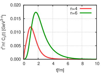
The main challenge in calculating, on the lattice, derivatives of the HVP function at zero virtuality is the fact that it requires determining, with high precision, the dominant, and notoriously noisy, and quark contributions to the electromagnetic current correlation function at large euclidean distances. This is particularly clear when these derivatives are obtained by computing moments, in euclidean spacetime, of the quark, electromagnetic two-point function, as described below, around Eq. (1). In Fig. 1 we plot the kernels of two such time-moments. They correspond to those needed for the first two derivatives of the HVP function at vanishing virtuality (the higher derivatives are obtained from higher moments). As the figure shows, the distances that need to be reached to reliably determine the slope and curvature are above and , respectively. Higher derivatives require even larger distances. Here we address this challenge by performing a high-precision calculation on lattices of spatial extent and of time extent , up to . This calculation yields a prediction of QCD for these quantities that can be compared to present [25] and future phenomenological determinations. We leave to a forthcoming paper the computation of the anomalous magnetic moment of the muon.
Simulations.– We employ a tree-level improved Symanzik gauge action [26] and a fermion action for four flavors of stout-smeared [27], staggered quarks. The up and down quark masses are treated as degenerate, their ratio to the strange quark mass is tuned to the vicinity of the physical point, which is defined from the Goldstone pion and kaon masses. The charm quark mass is fixed in units of the strange mass to [28]. More information on the action together with simulation and algorithmic details can be found in [29].
To set the physical mass point we use the isospin corrected pion and kaon masses, and , from [30]. To convert the lattice results into physical units, we use the pion decay constant [23] which is free of electromagnetic corrections and, to very good accuracy, equals to the decay constant in the limit [31]. This makes our definition of the physical point well defined in the isospin limit. In intermediate steps of the analysis we use the Wilson-flow-based [32] -scale [33]. For our finest lattice spacing the root mean squared pion mass is about 15% larger, than the Goldstone pion mass.
Table 1 lists the ensembles and the number of configurations used for quark-connected and disconnected measurements. A configuration corresponds to 10 unit length Rational Hybrid Monte Carlo (RHMC) [34] trajectories. The integration over the trajectory is improved with the gradient of the RHMC force [35, 36]. The topological charge undergoes sufficient number of tunnelings even on the finest lattices.
| #conf-conn | #conf-disc | |||
|---|---|---|---|---|
| 3.7000 | 0.134 | 1000 | 1000 | |
| 3.7500 | 0.118 | 1500 | 1500 | |
| 3.7753 | 0.111 | 1500 | 1500 | |
| 3.8400 | 0.095 | 2500 | 1500 | |
| 3.9200 | 0.078 | 3500 | 1000 | |
| 4.0126 | 0.064 | 450 | - |
Observables.– The hadron vacuum polarization is derived from the electromagnetic current , which is defined as , where is the unit of electromagnetic charge. From this we build the current-current correlator , in which we use the conserved lattice current at the source and sink. No renormalization is therefore necessary.
We split up the correlator in two different ways. First , where the first three terms contain the connected contractions for the light, strange and charm flavors, and the last contains the disconnected contractions. Flavor mixing terms arise only in the latter. We can also separate the correlator according to isospin symmetry, which is exact in our simulations: . Here the isospin singlet contribution is , whereas the isospin triplet one is . The lowest energy state contains three/two pions in the isospin singlet/triplet channel. This fact determines the behavior of the correlator for large separations.
We calculate the connected contributions to the correlators using point sources. We use the all-mode-averaging technique (AMA) of [37] and 768 random source positions on each configuration for the light quarks, 64 sources for the strange (except at where 128 were used) and 4 for the charm. To compute the quark-disconnected contributions, we apply AMA again, and exploit the approximate SU(3) flavor symmetry on around 6000 stochastic sources [38, 15]. We use random spatial wall sources, so only zero-momentum, time propagators are available. For the disconnected contribution of the charm we apply a hopping parameter expansion. The computer time required for this entire analysis is of the same order as the time needed for the generation of configurations.
The -th coefficient of a Taylor expansion of the vacuum polarization scalar, , around (i.e. ) can be written as , where each term is related to the respective, configuration-space correlator through moments [39, 14]
| (1) |
for , with and defined as and where is the size of the lattice in the -direction. In general the result depends on the choice of and . Three different averages, which are invariant under spatial cubic transformations, can be constructed: one which is an average over spatial moments, , of correlators of spatial currents, ; another, an average over spatial moments of correlators of timelike currents, ; a third, an average over time moments, , of correlators of spatial currents. We call these averages , and , respectively. In the disconnected case we only have the average. The averages and can be different, which is a consequence of the finite lattice size and the asymmetry .

In the case of the light and disconnected correlators the signal deteriorates quickly with increasing distance. In our analysis we consider the spatial moments, i.e. and , up to their full extent (ca. ). For the time-moment sums, , which can extend up to ca. , we introduce a cut in time. For times greater than we replace the correlator by an upper and a lower bound 11 1 We are grateful to Christoph Lehner for a discussion of this issue.. The connected light correlator is proportional to the isospin triplet one, whose lowest-energy contribution comes from a two-pion state. Therefore up to exponentially suppressed corrections in the correlator satisfies
| (2) |
where and is the energy of two pions, each with the smallest nonvanishing lattice momentum, for which we use . Typically the two bounds agree for , as seen for example on the top plot of Fig. 2. A similar conclusion is reached for the second derivative . In our analyses, we take on the light connected timelike correlators and average the two bounds to get the final result. Pion-pion interactions can change the smallest two-pion momentum from in that channel. Using the model of [40] and neglecting four-pion contributions, we determine the change in the momentum to be around 3%. We checked, that such a reduction of the momentum changes the result on by a small fraction of the statistical error.
The disconnected contribution alone can be constrained for large enough time separations, where the isospin singlet channel, dominated by three-pion states, can be neglected compared to the triplet, dominated by two-pion ones. Here we have
| (3) |
up to corrections exponentially suppressed in . This gives an upper and a lower bound on , which can be used to determine the time after which the two bounds agree within errors. At large , the connected strange and charm contributions in (3) are exponentially suppressed, and their presence does not make a difference when determining so we neglect them. In the bottom plot of Fig. 2 we show the upper and lower bounds on . In our analyses we average the two bounds for .
Results.– To obtain our final results in the continuum limit and at the physical point, we fit the lattice results to a function which depends on the pion and kaon masses and on the lattice spacing squared . Since the simulations were done around the physical point, a linear pion/kaon mass dependence is always sufficient. For the light, strange and disconnected contributions reasonable fit qualities can be achieved with a linear dependence.

| light | ||
|---|---|---|
| strange | ||
| charm | ||
| disconnected | ||
| total | ||
| I=1 FV corr. | ||
| total + FV |
We begin with the light quark contribution , paying special attention to the difference between the averages , and . Some ensemble show differences, but these are not significant statistically. If we assume no difference between the three averages and fit all ensembles and all three averages together in one fit, we get a reasonable fit quality . Also, if we include additional fit parameters describing the difference between the three averages, they come out zero within error bars. This remains true after dropping the coarser lattices from the fit, for which the two-pion, finite-volume effects are reduced by taste violations. Therefore we average over the combinations , and in this work and leave an investigation of differences for the future, when statistical errors are reduced. The upper panel of Fig. 3 shows the continuum extrapolation of . The coarsest lattice gives a value about 15% smaller than the continuum limit. The final central value and systematic error on the continuum limit are the mean and standard error of the Akaike-Information-Criterion-weighted distribution obtained by imposing four different cuts on lattice spacing (no cut, ) in the extended frequentist approach of [41, 42]. The results for the first and the second moments are given in Table 2.
The strange and charm quark contributions are plotted in the second and third panels of Fig. 3 and the respective continuum extrapolated values are given in Table 2. The strange channel has much smaller lattice artefacts than the light, since it is much less affected by taste violations. The difference between the continuum and the coarsest lattice is about 2%. For the charm the fit qualities are much worse, because the precision of the data is orders of magnitude better than for the lighter flavors. Here we fit only a random subset of 10 configurations, which increases the statistical error and leads to good fit qualities. Results on the coarsest lattice deviate by about 20% from the continuum limit.
The lattice spacing dependence of the disconnected is shown in the bottom panel of Fig. 3. We calculate the charm quark contribution to the disconnected term on the coarsest lattice: we find it to be of the total disconnected result, i.e. much smaller than the total disconnected statistical error. We therefore discard the charm from the disconnected term at all lattice spacings. has the largest lattice artefacts among the four contributions. Since we have one less lattice spacing available than in the connected cases, we apply only three cuts in . These extrapolations are also shown in Fig. 3.
The total result for is the sum of the four contributions. It has a combined error of about %. All of these results apply to a box size of and to the isospin symmetric case.
In the absence of a systematic study with simulations in a variety of volumes, only model estimates of finite-volume effects can be made. As argued in [43, 44], for large volumes those effects will be governed by pion contributions that can be computed in chiral perturbation theory (PT) [43]. Since the channel is dominated by three-pion exchange, the finite-size effects are expected to be smaller than those of the contribution, which are already small. Thus we consider only the latter. For all three index combinations, , and , we calculate the difference between the infinite and finite volume moments at one loop in PT. We then take the average of the maximum and the minimum differences as our central value, with an uncertainty given by the half distance between the maximum and minimum. We record these corrections for and in Table 2. For the first derivative the correction is on the level of , whereas on the second derivative it is of order . This correction increases rapidly with moment number, therefore we have chosen not to quote moments beyond the second one.
Concerning isospin breaking corrections, while little is known about how they modify the slope and curvature of the hadronic vacuum polarization function, more is known about their contribution to the anomalous magnetic moment of the muon. Compared to phenomenological determinations [8, 4, 5, 6], our calculation without QED is missing a number of effects 22 2 We are grateful to Maurice Benayoun and Fred Jegerlehner for very informative discussions on this subject.. Noting their contributions to in parentheses in units of , these effects are - ( from [45]) and - ( from [46, 47]) mixing, final state radiation ( from [2] with a 10% error added), and the ( from [4]) and ( from [4]) contributions. This leads to a correction of , i.e. 1.3% of the result for given in [4]. However, a competing effect enters. In our calculation without electromagnetism, the charged pion has a mass which is smaller than its physical value (see above). But a smaller charged-pion mass has the effect of enhancing the two-pion contribution to and thus leads to a correction whose sign is opposite to the correction associated with the sum of effects discussed above. Moreover, a phenomenological description based on data indicates that their magnitudes are very close [47]. Thus, we assume here that the total correction which has to be added to an isospin-limit determination of is , where we have taken the error to be of the typical size of the corrections themselves. Because of the dominant role which plays in determining , one expects a tantamount correction on that coefficient. Inferring the correction on is less direct, but we assume here that it is of the same size as for . Thus, we add of and to our results for these quantities, after they have been corrected for finite-volume effects.
Putting everything together we quote our final results for the first two moments in the last row of Table 2. Combining all four errors in quadrature, we obtain with a total uncertainty of and of .
Discussion.– It is interesting to compare these results with those in the literature. The only other lattice determination of on and , near the physical mass point, comes from a single, staggered simulation performed on a lattice with spacing [14, 48]. However, since the action used is different from ours and a comparison with our continuum limit results could be misleading, we choose not to exhibit such a comparison here.
The only phenomenological determination of the slope and derivative parameters, and , is the recent one of [25]. Taking their “data direct” results, which are obtained from an interpolation of data, and converting them to our conventions, we get and . These numbers can be compared to our final results, i.e. those given in the last row of Table 2. In absolute value, their result for is 0.3 combined standard deviations smaller than ours and for , 1.9 larger. The latter might be due to an underestimate of FV corrections in our determination of the second moment, or some problem with the experimental data used in the phenomenological analysis of [25].
Acknowledgments.– LL thanks M. Benayoun, C. Davies, F. Jegerlehner, C. Lehner, H. Leutwyler and E. de Rafael for very informative discussions. Computations were performed on JUQUEEN and JUROPA at Forschungszentrum Jülich, on Turing at the Institute for Development and Resources in Intensive Scientific Computing (IDRIS) in Orsay, on SuperMUC at Leibniz Supercomputing Centre in München, on Hermit at the High Performance Computing Center in Stuttgart. This project was supported by in part by the OCEVU Laboratoire d’excellence (ANR-11-LABX-0060) and the A*MIDEX Project (ANR-11-IDEX-0001-02), which are funded by the “Investissements d’Avenir” French government program and managed by the “Agence nationale de la recherche” (ANR), by the Gauss Centre for Supercomputing e.V and by the GENCI-IDRIS supercomputing grant No. 52275.
References
- [1] F. Jegerlehner, PHIPSI08, proceedings of the International Workshop on e+e- Collisions from phi to psi, Frascati (Rome) Italy, 7-10 April 2008, Nucl. Phys. Proc. Suppl. 181-182, 135 (2008), arXiv:0807.4206 [hep-ph] .
- [2] F. Jegerlehner and A. Nyffeler, Phys. Rept. 477, 1 (2009), arXiv:0902.3360 [hep-ph] .
- [3] J. P. Miller, E. de Rafael, B. L. Roberts, and D. Stöckinger, Ann. Rev. Nucl. Part. Sci. 62, 237 (2012).
- [4] M. Davier, A. Hoecker, B. Malaescu, and Z. Zhang, Eur. Phys. J. C71, 1515 (2011), [Erratum: Eur. Phys. J.C72,1874(2012)], arXiv:1010.4180 [hep-ph] .
- [5] K. Hagiwara, R. Liao, A. D. Martin, D. Nomura, and T. Teubner, J. Phys. G38, 085003 (2011), arXiv:1105.3149 [hep-ph] .
- [6] F. Jegerlehner, Proceedings, Workshop on Flavour changing and conserving processes 2015 (FCCP2015), EPJ Web Conf. 118, 01016 (2016), arXiv:1511.04473 [hep-ph] .
- [7] G. W. Bennett et al. (Muon g-2), Phys. Rev. D73, 072003 (2006), arXiv:hep-ex/0602035 [hep-ex] .
- [8] S. Eidelman and F. Jegerlehner, Z. Phys. C67, 585 (1995), arXiv:hep-ph/9502298 [hep-ph] .
- [9] T. Blum, Phys. Rev. Lett. 91, 052001 (2003), arXiv:hep-lat/0212018 [hep-lat] .
- [10] C. Aubin and T. Blum, Phys. Rev. D75, 114502 (2007), arXiv:hep-lat/0608011 [hep-lat] .
- [11] X. Feng, K. Jansen, M. Petschlies, and D. B. Renner, Phys. Rev. Lett. 107, 081802 (2011), arXiv:1103.4818 [hep-lat] .
- [12] M. Della Morte, B. Jager, A. Juttner, and H. Wittig, JHEP 03, 055 (2012), arXiv:1112.2894 [hep-lat] .
- [13] F. Burger, X. Feng, G. Hotzel, K. Jansen, M. Petschlies, and D. B. Renner (ETM), JHEP 02, 099 (2014), arXiv:1308.4327 [hep-lat] .
- [14] B. Chakraborty, C. T. H. Davies, G. C. Donald, R. J. Dowdall, J. Koponen, G. P. Lepage, and T. Teubner (HPQCD), Phys. Rev. D89, 114501 (2014), arXiv:1403.1778 [hep-lat] .
- [15] T. Blum, P. A. Boyle, T. Izubuchi, L. Jin, A. Jüttner, C. Lehner, K. Maltman, M. Marinkovic, A. Portelli, and M. Spraggs, Phys. Rev. Lett. 116, 232002 (2016a), arXiv:1512.09054 [hep-lat] .
- [16] B. Chakraborty, C. T. H. Davies, J. Koponen, G. P. Lepage, M. J. Peardon, and S. M. Ryan, Phys. Rev. D93, 074509 (2016a), arXiv:1512.03270 [hep-lat] .
- [17] T. Blum et al. (RBC/UKQCD), JHEP 04, 063 (2016b), arXiv:1602.01767 [hep-lat] .
- [18] T. Blum, M. Hayakawa, and T. Izubuchi, Proceedings, 30th International Symposium on Lattice Field Theory (Lattice 2012), PoS LATTICE2012, 022 (2012), arXiv:1301.2607 [hep-lat] .
- [19] F. Gray (New (g-2)), Nuclear physics. Proceedings, 25th International Conference, INPC 2010, Vancouver, Canada, July 4-9, 2010, J. Phys. Conf. Ser. 312, 102006 (2011), arXiv:1009.0799 [nucl-ex] .
- [20] M. Otani (E34), Proceedings, 2nd International Symposium on Science at J-PARC: Unlocking the Mysteries of Life, Matter and the Universe (J-PARC 2014): Tsukuba, Japan, July 12-15, 2014, JPS Conf. Proc. 8, 025008 (2015).
- [21] J. S. Bell and E. de Rafael, Nucl. Phys. B11, 611 (1969).
- [22] E. de Rafael, Phys. Lett. B736, 522 (2014), arXiv:1406.4671 [hep-lat] .
- [23] K. A. Olive et al. (Particle Data Group), Chin. Phys. C38, 090001 (2014).
- [24] C. Aubin, T. Blum, M. Golterman, and S. Peris, Phys. Rev. D86, 054509 (2012), arXiv:1205.3695 [hep-lat] .
- [25] M. Benayoun, P. David, L. DelBuono, and F. Jegerlehner, (2016), arXiv:1605.04474 [hep-ph] .
- [26] M. Luscher and P. Weisz, Commun. Math. Phys. 97, 59 (1985), [Erratum: Commun. Math. Phys.98,433(1985)].
- [27] C. Morningstar and M. J. Peardon, Phys. Rev. D69, 054501 (2004), arXiv:hep-lat/0311018 [hep-lat] .
- [28] C. T. H. Davies, C. McNeile, K. Y. Wong, E. Follana, R. Horgan, K. Hornbostel, G. P. Lepage, J. Shigemitsu, and H. Trottier, Phys. Rev. Lett. 104, 132003 (2010), arXiv:0910.3102 [hep-ph] .
- [29] R. Bellwied, S. Borsanyi, Z. Fodor, S. D. Katz, A. Pasztor, C. Ratti, and K. K. Szabo, Phys. Rev. D92, 114505 (2015), arXiv:1507.04627 [hep-lat] .
- [30] S. Aoki et al., (2016), arXiv:1607.00299 [hep-lat] .
- [31] J. Gasser and G. R. S. Zarnauskas, Phys. Lett. B693, 122 (2010), arXiv:1008.3479 [hep-ph] .
- [32] M. Lüscher, JHEP 08, 071 (2010), [Erratum: JHEP03,092(2014)], arXiv:1006.4518 [hep-lat] .
- [33] S. Borsanyi et al., JHEP 09, 010 (2012), arXiv:1203.4469 [hep-lat] .
- [34] M. A. Clark and A. D. Kennedy, Phys. Rev. Lett. 98, 051601 (2007), arXiv:hep-lat/0608015 [hep-lat] .
- [35] M. A. Clark, B. Joo, A. D. Kennedy, and P. J. Silva, Phys. Rev. D84, 071502 (2011), arXiv:1108.1828 [hep-lat] .
- [36] H. Yin and R. D. Mawhinney, Proceedings, 29th International Symposium on Lattice field theory (Lattice 2011), PoS LATTICE2011, 051 (2011), arXiv:1111.5059 [hep-lat] .
- [37] T. Blum, T. Izubuchi, and E. Shintani, Phys. Rev. D88, 094503 (2013), arXiv:1208.4349 [hep-lat] .
- [38] V. Gülpers, A. Francis, B. Jäger, H. Meyer, G. von Hippel, and H. Wittig, Proceedings, 32nd International Symposium on Lattice Field Theory (Lattice 2014): Brookhaven, NY, USA, June 23-28, 2014, PoS LATTICE2014, 128 (2014), arXiv:1411.7592 [hep-lat] .
- [39] X. Feng, S. Hashimoto, G. Hotzel, K. Jansen, M. Petschlies, and D. B. Renner, Phys. Rev. D88, 034505 (2013), arXiv:1305.5878 [hep-lat] .
- [40] M. Luscher, Nucl. Phys. B364, 237 (1991).
- [41] S. Durr et al. (Budapest-Marseille-Wuppertal), Science 322, 1224 (2008), arXiv:0906.3599 [hep-lat] .
- [42] S. Borsanyi et al. (Budapest-Marseille-Wuppertal), Science 347, 1452 (2015), arXiv:1406.4088 [hep-lat] .
- [43] C. Aubin, T. Blum, P. Chau, M. Golterman, S. Peris, and C. Tu, Phys. Rev. D93, 054508 (2016), arXiv:1512.07555 [hep-lat] .
- [44] A. Francis, B. Jaeger, H. B. Meyer, and H. Wittig, Phys. Rev. D88, 054502 (2013), arXiv:1306.2532 [hep-lat] .
- [45] M. Davier, A. Hoecker, G. Lopez Castro, B. Malaescu, X. H. Mo, G. Toledo Sanchez, P. Wang, C. Z. Yuan, and Z. Zhang, Eur. Phys. J. C66, 127 (2010), arXiv:0906.5443 [hep-ph] .
- [46] F. Jegerlehner and R. Szafron, Eur. Phys. J. C71, 1632 (2011), arXiv:1101.2872 [hep-ph] .
- [47] M. Benayoun and F. Jegerlehner, private communication, November 2016.
- [48] B. Chakraborty, C. T. H. Davies, P. G. de Oliviera, J. Koponen, and G. P. Lepage, (2016b), arXiv:1601.03071 [hep-lat] .