Neutrino-induced one-pion production revisited: the channel
Abstract
Understanding single pion production reactions on free nucleons is the first step towards a correct description of these processes in nuclei, which are important for signal and background contributions in current and near future accelerator neutrino oscillation experiments. In this work, we reanalyze our previous studies of neutrino-induced one-pion production on nucleons for outgoing invariant masses below 1.4 GeV. Our motivation is to get a better description of the cross section, for which current theoretical models give values significantly below data. This channel is very sensitive to the crossed contribution and thus to spin 1/2 components in the Rarita-Schwinger propagator. We show how these spin 1/2 components are nonpropagating and give rise to contact interactions. In this context, we point out that the discrepancy with experiment might be corrected by the addition of appropriate extra contact terms and argue that this procedure will provide a natural solution to the puzzle. To keep our model simple, in this work we propose to change the strength of the spin 1/2 components in the propagator and use the data to constraint its value. With this modification, we now find a good reproduction of the cross section without affecting the good results previously obtained for the other channels. We also explore how this change in the propagator affects our predictions for pion photoproduction and find also a better agreement with experiment than with the previous model.
pacs
25.30.Pt,13.15.+gI Introduction
New and more precise measurements of neutrino cross sections in the few GeV energy region have renewed interest in a better understanding of electroweak interactions on nucleons and nuclei. This interest comes from neutrino oscillation experiments and their need to reduce systematic errors to achieve the precision goals of the neutrino oscillation program, making new discoveries, like the CP violation in the leptonic sector, possible. Neutrinos are detected through their interactions with the nuclei that form part of the detectors. For nuclear physics, this represents a challenge because precise knowledge of neutrino oscillation parameters requires an accurate understanding of the detector responses, and it can only be achieved if nuclear effects are under control [1, 2, 3, 4, 5, 6]. Neutrino fluxes used in contemporary and near future long and short baseline experiments (T2K, NOA, MINERA, DUNE, …) are peaked in the 1–5 GeV energy domain, where weak pion production becomes one of the main reaction mechanisms [3]. Nuclear effects, arising from the fact that the reaction takes place inside of a nuclear medium, or from the final-state interactions (FSI) of the produced hadrons through their path across the nucleus will certainly need to be incorporated11 1 Weak pion production in dense matter is strongly affected by nuclear corrections, which might not be under control. As example of the theoretical difficulties faced, we refer the reader to the MiniBooNE flux-folded differential cross section data in mineral oil reported in Ref. [7], which cannot be described by the state of the art theoretical calculations of Refs. [8] and [9]. The latter approach is based in the chiral-inspired model of Ref. [10] for weak pion production reaction off nucleons, which will be updated in this work. MINERA pion production data for higher neutrino energies ( GeV) have recently become available [11, 12, 13] and show some appreciable inconsistencies, mostly in the magnitude of the cross sections, with MiniBooNE measurements. This is an open problem that deserves further discussion. Charged current pion production data from T2K will be an important check, since the neutrino energy range in this experiment is similar to that of MiniBooNE. .
Nevertheless, the first requirement to put neutrino induced pion production on nuclear targets on a firm ground is to have a realistic model at the nucleon level22 2 At this point, we should stress that the Rein-Sehgal model [14], used by almost all Monte Carlo generators, provides a really poor description of the pion electroproduction data on protons [15, 16]. Indeed, the model underestimates significantly the electron data, and it also reveals itself unsatisfactory in the axial sector at , where the divergence of the axial current can be related to the amplitude by PCAC (partial conservation of the axial current).. Data on neutrino pion production off nucleons all come from deuterium bubble chamber experiments carried out in the 1980’s at Argonne (ANL) [17] and Brookhaven (BNL) [18] national laboratories. The overall neutrino-flux normalizations of these measurements have been recently reanalyzed and corrected in Refs. [19, 20]. For antineutrinos, the measurements are of lower quality, and data on single nucleons are not available. Most of the models describe the pion production process by means of the weak excitation of the resonance followed by its strong decay into (pole mechanism depicted in the left-top diagram of Fig. 1), and in some occasions, incorporate background terms. The major part of the models includes also the weak excitation of higher resonances as intermediate states. Vector form factors are fixed from helicity amplitudes extracted in the analysis of pion electroproduction data, while the axial couplings are obtained from PCAC [4].
In this work, we pay a special attention to the cross section, for which current theoretical models give values significantly below data. Actually, this channel is certainly much worse described than the others, and , included in the ANL and BNL data sets. We reanalyze our previous study in Ref. [10] of neutrino-induced one-pion production on nucleons and show that this anomaly could be greatly improved by the addition of appropriate extra local terms. Such contributions are intimately related to the spin 1/2 degrees of freedom present in the Rarita-Schwinger (RS) propagator and greatly suppress the crossed mechanism (left-bottom diagram in Fig. 1). We find that the use of (almost) consistent couplings [21], which keep only the spin 3/2 contribution from the propagator, leads to an overall good description of the ANL and BNL data in all three available charge channels.
The work is organized as follows: After this introduction in Sec. II, we briefly review the most relevant ingredients of model of Ref. [10], updated in Refs. [9, 22], together with its predictions for the cross section for outgoing pion-nucleon invariant masses below 1.4 GeV. Next in Sec. III, we describe the propagator used in Ref. [10], and show that it is a Green function of the RS equation of motion. We also give its decomposition into a spin 3/2 part plus the rest. The latter is a nonpropagating spin 1/2 contribution that gives rise to contact interactions, at least in the limit of zero width. In Sec. IV, we describe the prescription of Ref. [21] to go from inconsistent to consistent couplings and show the effects of using consistent couplings in the evaluation of an amplitude where the appears as an intermediate state. The extension (modification) of our model is described in Sec. V, and the new results are presented in Sec. VI, where results for pion photoproduction are also given. The amplitude for this latter process derives from the vector part of our model for weak pion production, and it is described in the Appendix. Finally, in Sec. VII we summarize the main conclusions of this work.
II The model of Refs. [9, 10, 22]: Off diagonal Goldberger-Treiman relation, Watson’s theorem and the cross section
In Ref. [10], we developed a model for neutrino-induced one-pion production off the nucleon at low energies where, besides the dominant mechanism, we included also nonresonant contributions required by chiral symmetry. These chiral background terms were evaluated using a nonlinear SU(2) chiral Lagrangian and we supplemented them with well-known phenomenological form factors introduced in a way that respected both CVC (conservation of the vector current) and PCAC. As for the dominant contribution, the weak transition matrix element can be parametrized in terms of four vector form factors and four axial ones. is exactly zero from CVC, while the rest of the vector form factors were determined from pion electroproduction, and for them, we adopted the values in Ref. [23]. Axial form factors are mostly unknown. In fact, one uses the weak pion production process as a tool to extract information on the axial nucleon to resonance transition form factors. The term proportional to is the dominant one. Assuming the pion pole dominance of the pseudoscalar form factor, PCAC gives its value in terms of as , where is the lepton transfer four momentum and () the nucleon (pion) mass. We further adopted Adler’s model [24] in which one has , . We fitted to data assuming a modified dipole parametrization. The experimental data set consisted of the flux-averaged -differential cross section measured at ANL [17], which incorporated a kinematical cut GeV on the invariant mass of the final nucleon-pion pair. This was appropriate since our model ignored the contribution from higher mass resonances. From the fit we obtained . This result was at variance with the value derived from the off diagonal Goldberger-Treiman relation (GTR) that predicts –.
The disagreement with the GTR value got reduced in Ref. [25] where, following the work of Ref. [26], we included in our fit total cross sections measured at BNL [18], and we fully evaluated deuteron effects, the latter relevant since ANL and BNL data were actually obtained using a deuterium target. We had already noticed in Ref. [10] that the correct description of BNL cross sections required larger values. Our preference at the time for ANL data was due to the fact that they provided absolute -differential cross sections (as opposed to BNL, where only the shape was given) evaluated with a kinematical cut appropriate for our model. BNL cross section values are larger and they seemed to be incompatible with ANL ones. As it has recently been demonstrated in Ref. [19], where a reanalysis of both ANL and BNL data has been conducted, the discrepancies between the two data sets stem from their respective uncertainties in the neutrino flux normalization. In Ref. [25], in addition to the ANL flux-averaged -differential cross section, we included in the fit the three lowest neutrino energy total cross sections from BNL, and we considered the uncertainties on the neutrino flux normalizations as fully correlated systematic errors. Deuteron effects turned out to reduce the cross section by some 10% which agreed with previous estimates in Refs. [26, 27]. To compensate this reduction in the cross section, a roughly 5% larger value was needed. However, it was the consideration in the fit of BNL cross sections what was responsible for the larger change in . Assuming a simpler pure dipole form for , we obtained , a value closer to the GTR one33 3 In some fits carried out in [25], we unsuccessfully relaxed Adler’s constraints exploring the possibility of extracting some direct information on . We showed there that, the available low-energy data cannot effectively disentangle the different form-factor contributions..
In Ref. [9], and in order to extend the model to higher neutrino energies (up to 2 GeV), we added the contribution from the spin 3/2 nucleon resonance. This is the only resonance, apart from the , that gives a significant contribution in that energy region [28]. The corresponding vector and axial form factors for the transition current were taken, respectively, from fits to results in Refs. [29] and [30], respectively. A full account of the contribution can be found in the Appendix of Ref. [9].
Finally, in Ref. [22], we partially unitarized our model by imposing Watson’s theorem. This theorem is a result of unitarity and time-reversal invariance, and it implies that the phase of the electro or weak pion production amplitude is fully determined by the strong interaction elastic phase shifts . Imposing Watson restrictions in general is a difficult task, and thus in [22], we only paid attention to the dominant spin-3/2 isospin-3/2 positive-parity amplitude, where the direct excitation of the resonance occurs. Following the procedure suggested by M.G. Olsson in Ref. [31], we introduced independent vector and axial phases (two-dimensional functions of and ) to correct the interference between the dominant direct term and the nonresonant background. These extra phases were fixed by requiring that the total (resonance plus background contributions) amplitude in this dominant channel had the correct phase . Since this was not possible in a consistent way for all different terms that contribute to the amplitude in the multipolar expansion, we unitarized only the dominant vector and axial multipoles. Within this scheme, we performed two different fits in Ref. [22]. For fit A, we used the same input data as in Ref. [25] and described above. As a consequence of imposing Watson’s theorem the interference between the dominant direct contribution (left-top diagram of Fig. 1) and the background terms changed, and as a result, a larger value () for , in agreement now with the GTR prediction, was obtained. For fit B we used the results of Ref. [19]. As already mentioned, the authors of Ref. [19] reanalyzed ANL and BNL experiments producing data on the ratio between the and the charged current quasielastic (CCQE) cross sections measured in deuterium. In this way, the flux uncertainties present in the experiments cancel. They found a good agreement between the two experiments for these ratios. Then, by multiplying the cross section ratio by the theoretical CCQE cross section on the deuteron44 4 For that purpose, they used the prediction from GENIE 2.9 [32]., which is well under control, flux normalization independent pion production cross sections were extracted. We took advantage of these developments, and for fit B in Ref. [22], we considered the new data points. Since no cut in was imposed on this new data, we only used total cross sections for neutrino energies below 1 GeV. Besides, to constrain the dependence of the form factor, we also fitted the shape of the original ANL flux-folded distribution, where a GeV cut was implemented. For this fit, we obtained , similar to the result from fit A. The quality of the fit, the predictions for cross sections in other channels, as well as the values of the Olsson phases needed to satisfy Watson’s theorem were very similar in fits A and B.
The agreement of the theoretical predictions with data was also good for the total cross sections in other channels with one notable exception, the reaction shown in the right panel of Fig. 1, where theoretical predictions lie below experimental points. This is a common problem to other models [33, 34, 35, 36]55 5 Note that in Ref. [36], the theoretical predictions are below data when the cut GeV is implemented. Indeed, this work uses the SU(2) chiral model derived in Ref. [10], imposing GTR and including smaller contributions from other resonances different to the and the .. A special mention deserves the dynamical model of photo-, electro- and weak pion production initially derived in Ref. [33], and that has been recently further refined and extended to incorporate resonances and a larger number of meson-baryon states [34, 35]. Despite its theoretical and phenomenological robust support, satisfying unitary constrains and fulfilling thus Watson’s theorem, this model provides a description of the channel, only slightly better [37] to that shown here in the right panel of Fig. 1.


As can be deduced from the explicit expressions given in Ref. [10], the reaction gets a large contribution from the crossed mechanism (left-bottom diagram in Fig. 1), and thus it is very sensitive to the spin 1/2 components present in the RS covariant propagator. Indeed, besides the propagator, the numerical factors of the (direct crossed) mechanisms are ( ), (), and () for the , , and channels, respectively66 6 Note that the coefficients quoted in a similar discussion in Ref. [22] were wrong by an overall factor.. Thus, isospin invariance implies that the largest (smallest) contribution of the crossed mechanism occurs in the () channel, while the largest (smallest) contribution of the direct mechanism in contrast is found in the () amplitude.
The RS covariant propagator, with its lower spin components, is considered to be incorrect in Ref. [38], where the authors advocate the use of the pure spin 3/2 propagator of Behrends and Fronsdal [39]. The opposite view is adopted in Ref. [40], where the pure spin 3/2 propagator is considered incorrect since it does not satisfy the appropriate Green function equation. In Ref. [41], it is argued that off shell terms of lower spin can naturally appear in the construction of propagators, and such terms explain, for instance, the decay of a spinless pion through an intermediate vector meson, without violating the conservation law of angular momentum. It is only because the vector propagator has an off shell spin 0 part that the charged pion can decay [41, 40, 42]. What is also true is that those lower spin terms are always nonpropagating giving rise to pure contact interactions. In Refs. [43, 44, 21], the approach is somewhat different. There, the authors arrive at a pure spin 3/2 contribution from the propagator by selecting consistent couplings. These are derivative couplings that preserve the gauge invariance of the free massless spin 3/2 Lagrangian. In Ref. [21], it is shown how to obtain consistent couplings from inconsistent ones by just a redefinition of the spin 3/2 field. The difference amount to contact terms that in this approach are responsible for the contribution of the extra lower-spin degrees of freedom. However, as already acknowledged in Ref. [43], and very recently reanalyzed in Ref. [45], consistent couplings cannot be kept in the presence of electromagnetic interactions. This is so since any derivative on the field gives rise through minimal substitution to a new nonderivative term.
Our approach to this problem is conceptually different, based on the perspective of an effective field theory, and it is motivated by the discussion in Ref. [21]. In this latter reference, it is argued that i) the use of consistent or inconsistent couplings will provide the same physical predictions as far as all relevant contact terms allowed by the underlying symmetries are included in both cases, and ii) the strength of the contact terms will have to be fitted to experiment. According to this, in this work, we propose a minimal modification of our model, in which the contact terms that derive from the spin 1/2 part of the propagator are multiplied by an extra parameter (low energy constant), that will be fitted to data.
III Rarita-Schwinger propagator
The RS Lagrangian of the free massive spin 3/2 reads [21] [we particularize for the resonance case],
| (1) |
where represents the RS field for the and
| (2) |
with and . The Lagrangian in Eq. (1) corresponds to the parameter in the discussion of Eq. (2) of Ref. [40] (note that the physical properties of the free field are independent of this parameter). The Euler-Lagrange equation reads
| (3) |
which leads to the set of equations
| (4) |
The corresponding RS propagator is
| (5) |
| (6) |
In the zero width limit (, i.e., when dealing with a stable particle), the above propagator gives the Green function of the RS equation of motion
| (7) |
with the Fourier’s transform of . This result follows trivially from
| (8) |
which can be obtained after a little of Dirac algebra.
The operator can be rewritten as [44]
| (9) |
with
| (10) |
satisfies the relations
| (11) |
from where one concludes that is the spin-3/2 projection operator.
Finally, we would like to stress that Eq. (9) shows that in the RS propagator of Eq. (5), only the spin-3/2 degrees of freedom propagate, while the controversial spin-1/2 contributions give rise to contact background terms. (This is strictly true in the zero width limit where the factor in Eq. (9) cancels the denominator of the propagator.) As we will discuss below, the total strength of the contact terms is undetermined in an effective chiral expansion, and it needs to be determined from experiment.
IV Consistent interactions: the prescription of Ref. [21]
The kinetic term of the free RS Lagrangian in Eq. (1) is invariant under the gauge transformation
| (12) |
with a spinor. It is argued in Refs. [43, 44] that any interaction term that respects this symmetry does not change the degrees of freedom content of the free theory, where the constraints on guarantee that it indeed describes spin 3/2 particles. Couplings respecting this symmetry are called consistent ones. In the case of linear couplings of the form
| (13) |
where is any current coupled to , the invariance of the Lagrangian under the gauge transformation requires the current to be conserved. If that is not the case, the coupling is called inconsistent. The transformation of this latter coupling into a consistent one can be achieved via a redefinition of the field
| (14) |
This transformation modifies the linear coupling
| (15) |
and gives rise to an additional contact interaction Lagrangian, , independent of the RS field (see Ref. [21] for details on ). By selecting
| (16) |
where
| (17) |
one has that the new total current coupled to the is
| (18) |
which is indeed conserved.
Apart from a total divergence of no consequence, Eq. (15) can be rewritten as
| (19) |
This is the prescription described in Ref. [21] to transform an inconsistent coupling into a consistent one. The description in terms of the original or the modified Lagrangians is equivalent at the level of the matrix.
It is further argued in Ref. [21] that, within chiral perturbation theory (ChPT), any linear spin-3/2 coupling is acceptable. This is so since the additional contact terms, which provide the equivalence between inconsistent and consistent couplings, have to be included in both situations with arbitrary coefficients that have to be fitted to some experimental input. Thus, it is only the value of the coefficients of the contact terms that change. In this respect, the spin-1/2 contributions in the RS propagator, that give rise to pure contact terms, can be totally eliminated and their effects reabsorbed into the values of some of the low-energy constants of the additional zero-range couplings. According to Ref. [21], it is preferable to use consistent interaction terms, supplemented with the adequate contact interactions, in the analysis of the separate contributions due to spin 3/2 degrees of freedom versus the rest.
To see the effect of the use of consistent interactions, let us consider a process driven by the excitation of the and its subsequent decay into some final particles. This mechanism is depicted in the left panel of Fig. 2, and it is determined by the currents and that couple the to the initial and final particles, respectively, and that we assume to be of the inconsistent type.
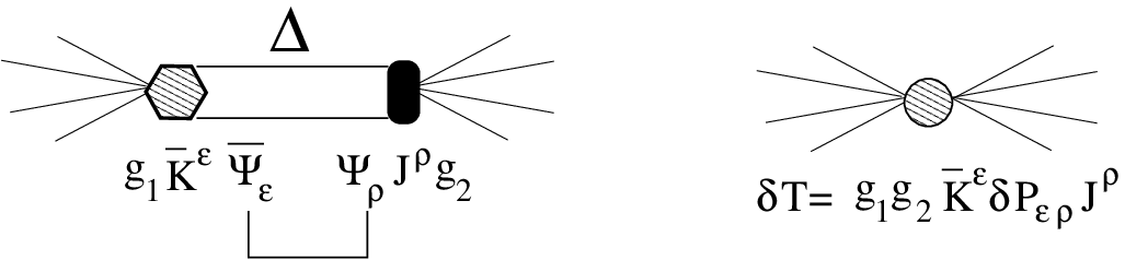
In the zero width limit, the amplitude for the process would be
| (20) |
while using the consistent currents and , one would get
| (21) | |||||
| (22) | |||||
| (23) |
This result follows from the antisymmetry of the tensor that guaranties that,
| (24) | |||||
and some further Dirac algebra77 7 In Eq. (24), the tensor in gives the final result, , while the part produces an antisymmetric tensor in the and indices whose contribution vanishes when contracted with the symmetric term..
By comparing Eqs. (20) and (23), we see that the use of consistent couplings induces the replacement
| (25) |
in the Feynman amplitudes. Note that the factor in front of corrects for the ill-defined infrared behaviour of the latter operator. From Eq. (9) we see that and differ in terms that vanish on shell (),
| (26) | |||||
| (27) |
and thus, the amplitudes and differ in a contact (nonpropagating) term ,
| (28) |
The discussion above amounts to admit that the actual size of a contact term like is in fact undetermined, since the contact terms that appear in the effective chiral expansion are not fixed, and need to be fitted to experiment. Hence the use of consistent or inconsistent couplings should not produce any difference, as long as the needed contact terms are phenomenologically determined.
IV.0.1 The coupling
For the case of the coupling, in Ref. [10] we took
| (29) |
with the strong coupling constant, the pion mass, and the nucleon and pion fields88 8 In our convention, creates a from the vacuum or annihilates a , whereas the field creates or annihilates a ., and the isospin transition operator defined such that its Wigner-Eckart reduced matrix element is equal to one. The width that results from the above vertex, assuming an onshell at rest and with mass , i.e., , is given by99 9 In the expression of Eq. (45) of Ref. [10], the factor was approximated by .,
| (30) |
where and are the mass and energy of the final nucleon and the final pion momentum, respectively in the rest frame. Using isospin averaged masses and the value MeV [48] we obtain to be compared to the value 2.14 that we have been using so far. The use of a consistent coupling would lead to the inclusion of an additional multiplicative factor .
To end this section, we would like to devote a few words to the use of a more general interaction of the form [40]
| (31) |
In diagrams with an intermediate , and because = 0, the term will always give rise to contact contributions which, as argued above, need to be phenomenologically determined. Hence, without lost of generality, one can ignore these off shell terms as far as all relevant contact interactions are taken into account1010 10 In this context, the inconsistency between the free propagator and the Lagrangian referred to in Refs. [42, 46] would no longer be relevant..
V Extension of the model of Refs. [10, 9, 22]
Aiming at improving the description of the channel, we open the possibility of supplementing the model of Refs. [10, 9, 22] with some additional contact terms. To keep the model simple, we introduce just one undetermined low energy constant (LEC), , that enters in a modification of the propagator compatible with ChPT,
| (32) |
with the operator defined in Eq. (27). The introduction of this LEC induces two new terms in the model that come from the direct () and crossed pole () amplitudes. [Note that there no exists an unequivocal relation between the LEC and the parameter introduced in Eq. (31), and thus effects produced by the latter cannot be completely accounted by the inclusion of these two new terms.]
So far, the values and would correspond to the use of inconsistent and consistent couplings. We now reintroduce in the denominator of the propagator in Eq. (32) the imaginary part , where for we use Eq.(30) with the new value. Note that the width is zero for the term, while we expect the direct contribution to be largely dominated by the resonant propagator, being there the influence of the term quite small. However, we foresee that the contribution of this latter term could be relevant in the amplitude, because in that case the is largely off shell.
It is worth stressing that the nondiagonal GTR is not affected by the changes and it predicts
| (33) |
that for MeV and the isospin averaged value that we use
results in .
In principle one could also modify the terms included in
our model (see Ref. [9]) along the lines
described above and introduce an extra parameter. However, since the
exchange contributions play a minor
role, the effect of these latter modifications would
be much less important, and we shall ignore them.
With the modification in the contributions, we repeat the fit B carried out in Ref. [22]. There is a total of four best fit parameters: the LEC , , and , that determine the axial form factor for which we assume a dipole form
| (34) |
and the normalization parameter of the ANL differential cross section introduced in Ref. [22]. In addition and to increase the sensitivity on the new parameter, we now also include in the fit data for the reaction. We thus minimize the following
| (35) | |||||
where . The differential cross section values are the flux averaged measurements carried out at [17] (ANL) and they contain a GeV cut in the final pion-nucleon invariant mass. This data set serves the purpose of constraining the dependence of the axial form factor. The role played by the parameter is to allow fitting only the shape of this distribution. The total ANL and BNL cross sections included in the fit are collected in Table II of Ref. [22]. They have been taken from the reanalysis of Ref. [19], where flux uncertainties in the original ANL and BNL data have been eliminated. Since they do not include a cut in , we only consider cross sections for neutrino energies GeV. Finally, for the total cross section, we take also the results of the reanalysis of the ANL data conducted in Ref. [20] and shown in Table 1. In this latter case, the data do contain a GeV cut.
| (GeV) | Expt. | ||
|---|---|---|---|
| 0.400 | 0.010 | 0.006 | ANL |
| 0.625 | 0.070 | 0.014 | ANL |
| 0.875 | 0.121 | 0.022 | ANL |
| 1.125 | 0.110 | 0.024 | ANL |
| 1.375 | 0.122 | 0.033 | ANL |
VI Results
VI.1 Pion production by neutrinos
The best fit parameters resulting from the new fit are
| (36) |
The new is dominated by the reaction that gives rise to about of the total. is now larger by 3.5% than that found in Ref. [22], and it is in excellent agreement with the GTR value. The parameter is a measure of the neutrino flux uncertainty in the ANL experiment. Its value is in agreement with the 20% uncertainty assumed for our fit A in Ref. [22] and the fits in Refs. [26, 25].
In Fig. 3, we compare the fitted data and the new theoretical results. For comparison we also show the results from fit B carried out in Ref. [22]. The shape for the flux averaged differential cross section is shown in the upper left panel. Both fits give almost identical results, as it is also the case for the total cross section, depicted in the upper right panel, where some minor differences can be only seen for the larger neutrino energies.


In the lower panel, we show the cross section. The new theoretical results are very different from the ones obtained from fit B in Ref. [22], and they are now in a much better global agreement with experimental data. The modifications introduced in the contributions, that amount to the introduction of new contact terms controlled by the fitted LEC , are crucial for this. Without those, one can not reproduce the cross sections without worsening the agreement with data in other channels.
Results for the total and cross sections are given in Fig. 4. We find a good global agreement with data and only very minor differences with the results obtained from fit B carried out in Ref. [22].
The brown and gray theoretical bands in Figs. 3 and 4 show the sensitivity of the predicted cross sections to the errors on the the best-fit parameters and the LEC , respectively. In this latter case, only the channel is strongly affected when varying . This was not unexpected, since the cross section has a large contribution form the CP amplitude, and thus, it is very sensitive to the spin 1/2 part of the propagator, which strength is now controlled by the parameter .
The Olsson phases needed to satisfy Watson’s theorem are presented in Fig. 5. We have selected the scales in order to allow a direct comparison with those obtained in Ref. [22], which are shown in Fig. 3 of that reference. We now find much smaller values, always below 20o, and at the peak (left panel in Fig. 5) axial (vector) phases remain quite small and below 5o (10o) for the whole range GeV of values shown in the plot. This means that the present model without the phases is closer to satisfying unitarity than the one in Ref. [22].


Finally, we pay attention to the best-fit value quoted in Eq. (36) for the LEC . It is compatible with , within errors, but however we should point out that does not correspond exactly to a consistent coupling. This is because of the width, and thus even for , we have
| (37) | |||||
The first term in Eq. (37) corresponds to the prescription for consistent interactions advocated in Refs. [43, 44, 21]. The second one, that vanishes for the CP amplitude, provides complex corrections to the direct contribution, which induce changes in the Olsson phases. Indeed, we have checked that if the second term in Eq. (37) is neglected, one finds also an improved description of the data, as compared to the case, and just a bit worse than that presented here in Fig. 3. However, the needed Olsson phases turn out to be larger than those depicted in Fig. 5, being only slightly different to the ones found in Ref. [22], where the LEC was set to zero. Note that the factor, in front of the first term of Eq. (37), drastically suppresses the CP contribution, because in this mechanism the is largely off shell, with much smaller (in modulus) than .
If one looks in more detail at the results for the cross section shown in the lower panel of Fig. 3, one sees that, though we obtain a global good agreement, the model underestimates the experimental (central) values below 0.9 GeV, while for higher energies it overestimates the data. This is also true, with some exceptions, for the and channels depicted in Fig. 4. In fact, the model fails to provide a reasonable description of the central values below 1 GeV for those channels, using realistic values of the fitted parameters as we will see later. This is the reason why to better determine the parameter , we included data above 1 GeV, and then we had to implement the cut in . The situation is different for the case, where we provide a good reproduction of the data for neutrino energies below 1 GeV. One might, however, look at the predictions of the model for the cross sections, with the GeV cut, at higher energies. The comparison of the model results with data, up to GeV for the neutrino energy, is now shown in Fig. 6.

We find an overall reasonable description of the reanalyzed ANL and BNL cross sections, though the model also overestimates the central values for neutrino energies in the range – GeV, as it occurred in the other channels.
Part of this discrepancy could be perhaps accounted for by including a phenomenological form factor to regularize the possible unphysical behavior of the tree-level amplitudes in the kinematic regions far from the peak of the resonance [49]. The effects of such form factor, with the form and parameters used in [49], on the GeV cross sections could be seen in Fig. 18 of this latter reference, and they would certainly improve the description exhibited in Fig. 6. This would also improve our reproduction of the and data at energies above 1 GeV. Results below 1 GeV will be affected to a much lesser extend, while the effects on the flux-folded differential cross section could be mostly reabsorbed into the flux parameter. This is certainly a topic that is worth analyzing in future work, paying also an special attention to its possible interference/interplay with the partial unitarization implemented in our model through the Olsson phases [22]. When considering higher neutrino energies, it would be also advisable to study the effects produced by the assumption of the Adler’s constrains on the axial and form factors. The contributions driven by these latter form factors are not relevant at the low values accessible when the neutrino energy is below 1 GeV [25], but they might need to be considered more carefully, especially in the channel, when higher neutrino energies are examined.
Nevertheless, we have also carried out a best fit taking into account the GeV cross sections depicted in Fig. 6 instead of those below 1 GeV, shown in the upper right panel of Fig. 3. The new best fit parameters differ from those quoted in Eq. (36) in one (, ) or two () sigmas1111 11 The largest changes occur for and . The first of these parameters now takes values of around 1.07 leading to smaller cross sections. This needs to be compensated by a change of 15% in the normalization parameter , which is now around , to avoid spoiling the description of the flux averaged differential cross section included in the fit.. The new fit is, in our view, somehow unsatisfactory, because the resulting model appreciably underestimates the cross section data obtained at 0.7 and 0.9 GeV when no cut on is imposed. It is, however, precisely at these low energies where the model, inspired in a chiral expansion, should perform best. A word of caution must be said here. For neutrino energies below 1 GeV, the GeV cut does not lead to appreciable effects on the cross sections obtained within our model. This is in accordance with the data shown in Table III of Ref. [17] (ANL), where up to 1 GeV, there is almost no difference between data reported with and without the cut. This should be expected, since below 1 GeV there is little phase space available for GeV. However, as seen in Fig. 6, both ANL and BNL reanalyzed data for 0.9 GeV are significantly smaller when the cut GeV is taken into account. Thus, it seems to be a certain degree of inconsistency between the two data sets (with or without the GeV cut) below 1 GeV. As a result, we can fit the parameters in our model to reproduce one or the other set of cross sections, but not both at the same time. We preferred to use the reanalyzed data without the GeV cut since their extraction seem to suffer from less uncertainties1212 12 As stated in Ref. [20], to get the reanalyzed GeV cross sections, the ratio of reanalyzed to published cross sections obtained without the cut is used..
Finally, we have also explored the possibility of fitting only data below 1 GeV and with no GeV cut applied. To that end, we have included in the fit , and data in this neutrino energy range taken from Ref. [20]. In this new fit, the parameter significantly departs from (propagation of only spin 3/2 degrees of freedom in the CP term) and becomes closer to , while is about 1.23, now even above the GTR prediction. However the normalization parameter turns out to be 1.35, a value too large to be accommodated within the ANL flux uncertainties. Besides, one obtains , which is much worse than for our preferred fit in Eq. (36).
Thus, we consider the fit of Eq. (36) a sensible option, given the somehow uncertain situation, and that it leads to a remarkable description of the pion photoproduction data off the nucleon, as we will discuss next.
VI.2 Pion photoproduction
Since in Ref. [22], we showed results for pion photoproduction, it is relevant to see also for this case the effect of the modification introduced in the propagator. Amplitudes for pion photoproduction derive directly from the vector part of our model for weak pion production by neutrinos and they are extensively discussed in the Appendix. As for the case of neutrino production, the model is also partially unitarized by imposing Watson’s theorem on the dominant vector multipole, now evaluated at . What we will show are pure predictions of the model without any readjustment of parameters or vector form factors. In Fig. 7 we present results for total cross sections that we compare to data taken from the George Washington University SAID database [51]. On the theoretical side, we compare the predictions obtained with the present model (red solid lines) with the results obtained without the modification of the spin 1/2 component of the propagator (black dashed lines), the latter corresponding to setting . The description of the data is better in the current modified case, with close to . The theoretical bands show the sensitivity of the results with respect to the parameter, when it is varied within the errors quoted in Eq. (36). To get a better reproduction of the cross sections above the resonance region, the model would have to be enlarged by the addition of extra resonance contributions relevant for the case of electro- or photoproduction.


VII Summary and conclusions
We have improved our model of Refs. [10, 9, 22] by including two extra contact terms1313 13 The correction in the propagator of Eq. (32) induces contact interactions both for the and amplitudes in the original model of Refs. [10, 22].. This has been motivated by the failure of present theoretical approaches to describe the total cross section data. As shown in Ref. [10], this channel has a large contribution from the CP mechanism and it is thus very sensitive to the spin 1/2 components in the propagator. This spin 1/2 part is nonpropagating and it gives rise to contact terms. Contact terms appear naturally within effective field theories, and in particular in ChPT, as counterterms with unknown strengths. Indeed, the coefficients of the contact terms have to be ultimately fitted to experiment. Aiming at keeping our model simple, we have just introduced only one new parameter, , that controls the strength of the contact terms generated by the spin 1/2 part of the propagator. To constraint its value, we have also included cross section data in the fit. The description of this channel considerably improves, without affecting the good results we had already obtained in Refs. [10, 22] for the other channels. Since the fitted value of is compatible with , we find that the crossed pole amplitude is substantially suppressed and that consistent couplings [43, 44, 21] are preferred. Besides, the new Olsson phases needed to satisfy Watson’s theorem are now much smaller than those obtained in Ref. [22] for the case, indicating that the present version without the phases is closer to satisfying unitarity. Yet, the is now larger by 3.5% than that found in Ref. [22], and it is in remarkable agreement with the GTR prediction.
We have also explored how this change in the propagator affects our predictions for pion photoproduction. We also find now a better agreement with experiment compared to the case where the LEC was set to zero.
Finally, we should mention that FSI effects on single pion production off the deuteron might induce corrections on the nucleon spectator approximation. This approximation is used to extract the pion production cross sections on the nucleon from the data on the deuteron. These effects have not been addressed in this work. However, it has been argued [52, 53] that they might be of special relevance precisely in the channel, and that the ANL and BNL data on the deuterium target might need a more careful analysis with the FSI’s taken into account. For such a reanalysis to be meaningful, it will be mandatory to incorporate the kinematical cuts implemented in the old experiments to properly separate the three reaction channels (, and ), since these cuts were designed to minimize the corrections to the spectator hypothesis. Nevertheless, the existence of some FSI effects will not exclude the solution to the puzzle offered here, and based on the possibility of adding phenomenological contact terms. It is certainly natural within the context of effective field theories.
Acknowledgements.
We acknowledge discussions with A. Mariano and A. Pich. This research has been supported by the Spanish Ministerio de Economía y Competitividad and European FEDER funds under Contracts No. FPA2013-47443-C2-2-P, No. FIS2014-51948-C2-1-P, No. FIS2014-57026-REDT. and No. SEV-2014-0398, and by Generalitat Valenciana under Contract No. PROMETEOII/2014/0068.Appendix A Model for pion photo- and electroproduction off the nucleon
Our model for pion photo or electroproduction off the nucleon derives directly from the vector part of that constructed for weak pion production by neutrinos. Thus, it includes all the contributions depicted in Fig. 8: the resonant direct and crossed pole terms (P and CP, respectively) and the background terms required by chiral symmetry. The latter ones include direct and crossed nucleon pole (labeled as NP and CNP), contact (CT) and pion-in-flight (PF) terms. Besides we also consider the direct and crossed pole terms (DP and CDP, respectively).

In the notation of Ref. [10], the quark level electromagnetic current is given by1414 14 We ignore the contribution from heavy quarks.
| (38) |
This can be written as the sum of an isoscalar and an isovector pieces
| (39) | |||||
| (40) |
with and , where are the three Pauli matrices.
In the same notation the vector part of the charged weak current reads
| (41) |
with . We could relate the matrix elements of the isovector part of the electromagnetic current with those of . To that end, we express the physical nucleon-pion states in terms of states with well-defined total isospin,
| (42) |
and then we can obtain1515 15 For a tensor operator , we use the Wigner-Eckart theorem with the convention (43) with a Clebsch-Gordan coefficient and the reduced matrix element.
| (44) | |||||
from where
| (45) |
These two reduced matrix elements determine all matrix elements of the isovector part of the electromagnetic current. As an example, we evaluate1616 16 Note the factor difference in the definition of and .
| (46) | |||||
Similarly,
| (47) |
Since the exchange contributions of Fig 8 are purely isovector, and denoting by the matrix elements of the electromagnetic current, we thus get1717 17 The Feynman amplitude will be proportional to , with the photon polarization vector and , the dimensionless proton electric charge, with .
where , , , and are the incoming photon and nucleon and the outgoing pion and nucleon four momenta.
To compute the nonresonant amplitudes, we pay attention to the electromagnetic current associated to the Lagrangian of the SU(2) nonlinear model derived in Ref. [10]. It reads,
| (59) |
with , MeV, and the nucleon and pion fields already introduced in Sec. IV.0.1. We have only kept those terms contributing to one pion production in the absence of chiral loop corrections. Thus, within our framework, and besides the excitation of the and the , the model for the reaction would consist of direct and crossed nucleon pole, contact and pion-in-flight terms, as shown diagrammatically in Fig. 8. We see that neither the pion-in-flight nor the contact terms contribute for photoproduction, which implies in turn that they are purely isovector. Thus, we get for these two contributions
For the proton and neutron Dirac electromagnetic form factors, we use the parametrization of Galster et al. [50], as we did in Ref. [10] for weak pion production.
To account for direct and crossed nucleon pole contributions, we need to consider, in addition to the isovector part, the isoscalar part of the electromagnetic current. For the isoscalar part of the electromagnetic current we have from Eq. (42)
| (66) |
Using the current of Eq. (59), supplemented by including i) the dependence induced by the Dirac form factors and ii) the magnetic contribution in the vertex [with the corresponding magnetic form factors , for which we also use the Galster parametrization], we find [10]
| (68) | |||||
with
| (69) |
where we have made use of the cancellation of the isovector contributions in the difference .
Taking also into account the isovector contributions, we get the following direct and crossed nucleon pole amplitudes:
with
| (88) |
One can check that CVC is preserved by the nonresonant amplitudes.
Finally, we give the expressions for the DP and CDP terms. The isovector parts are determined, as for the case of the , in terms of the matrix elements of the weak vector current that appear in the Appendix of Ref. [9]. They are given by
with MeV, and
| (100) | |||||
The corresponding vector form factors are given in Ref. [9] and they are
obtained from a fit to results in Ref. [28].
The value of the strong coupling is determined from the partial decay width to be GeV-1. This partial decay width is given, for , by
| (102) |
with . For we took 61% of 115 MeV. For the total width we use
| (103) |
where for we assumed an wave decay and took
| (104) |
with and
.
As for the matrix elements of the isoscalar part of the electromagnetic current associated to the , we make use of the relations given in Eq. (66) and the expression for given in Ref. [9]. Thus, we obtain
with
| (115) |
The isoscalar form factors are given in Ref. [9]. For them we use the same functional form as for the while their values at have been taken from Ref. [29].
Finally, the differential cross section in the laboratory (LAB) frame for real photons is obtained from the amplitudes as
| (116) |
The energy conservation Dirac delta fixes the pion polar angle in the LAB frame as
| (117) |
In addition, the average and sum over the initial and final nucleon spins in Eq. (116) is readily done thanks to
| (118) |
where the spin dependence of the Dirac’s spinors is understood and is a matrix in the Dirac’s space for each value of the Lorentz index .
References
- [1] H. Gallagher, G. Garvey and G. P. Zeller, Ann. Rev. Nucl. Part. Sci. 61 (2011) 355.
- [2] J. G. Morfin, J. Nieves and J. T. Sobczyk, Adv. High Energy Phys. 2012 (2012) 934597.
- [3] J. A. Formaggio and G. P. Zeller, Rev. Mod. Phys. 84 (2012) 1307.
- [4] L. Alvarez-Ruso, Y. Hayato and J. Nieves, New J. Phys. 16 (2014) 075015.
- [5] U. Mosel, Ann. Rev. Nucl. Part. Sci. 66 (2016) 171.
- [6] T. Katori and M. Martini, arXiv:1611.07770 [hep-ph].
- [7] A. A. Aguilar-Arevalo et al. [MiniBooNE Collaboration], Phys. Rev. D 83 (2011) 052009.
- [8] O. Lalakulich and U. Mosel, Phys. Rev. C 87 (2013) 014602.
- [9] E. Hernández, J. Nieves and M. J. V. Vacas, Phys. Rev. D 87 (2013) 113009.
- [10] E. Hernández, J. Nieves and M. Valverde, Phys. Rev. D 76 (2007) 033005.
- [11] B. Eberly et al. [MINERvA Collaboration], Phys. Rev. D 92 (2015) 092008.
- [12] T. Le et al. [MINERvA Collaboration], Phys. Lett. B 749 (2015) 130.
- [13] C. L. McGivern et al. [MINERvA Collaboration], Phys. Rev. D 94 (2016) no.5, 052005 doi:10.1103/PhysRevD.94.052005.
- [14] D. Rein and L. M. Sehgal, Annals Phys. 133 (1981) 79.
- [15] K. M. Graczyk and J. T. Sobczyk, Phys. Rev. D 77 (2008) 053001.
- [16] T. Leitner, O. Buss, U. Mosel and L. Alvarez-Ruso, PoS NUFACT 08 (2008) 009.
- [17] G. M. Radecky et al., Phys. Rev. D 25 (1982) 1161; Erratum: [Phys. Rev. D 26 (1982) 3297].
- [18] T. Kitagaki et al., Phys. Rev. D 34 (1986) 2554.
- [19] C. Wilkinson, P. Rodrigues, S. Cartwright, L. Thompson and K. McFarland, Phys. Rev. D 90 (2014) 112017.
- [20] P. Rodrigues, C. Wilkinson and K. McFarland, Eur. Phys. J. C 76, 474 (2016).
- [21] V. Pascalutsa, Phys. Lett. B 503 (2001) 85.
- [22] L. Alvarez-Ruso, E. Hernández, J. Nieves and M. J. V. Vacas, Phys. Rev. D 93 (2016) 014016.
- [23] O. Lalakulich and E. A. Paschos, Phys. Rev. D 71 (2005) 074003.
- [24] S. L. Adler, Annals Phys. 50 (1968) 189.
- [25] E. Hernández, J. Nieves, M. Valverde and M. J. Vicente Vacas, Phys. Rev. D 81 (2010) 085046.
- [26] K. M. Graczyk, D. Kielczewska, P. Przewlocki and J. T. Sobczyk, Phys. Rev. D 80 (2009) 093001.
- [27] L. Alvarez-Ruso, S. K. Singh and M. J. Vicente Vacas, Phys. Rev. C 57 (1998) 2693.
- [28] T. Leitner, O. Buss, U. Mosel and L. Alvarez-Ruso, Phys. Rev. C 79 (2009) 038501.
- [29] T. J. Leitner, “Neutrino-nucleus interactions in a coupled-channel hadronic transport model”. Ph.D thesis, University of Giessen, 2009. A copy can be retrieved from the webpage https://www.uni-giessen.de/fbz/fb07/fachgebiete/physik/einrichtungen/theorie/inst/theses/dissertation/neutrino-nucleus-interactions-in-a- coupled-channel-hadronic-transport-model.
- [30] O. Lalakulich, E. A. Paschos and G. Piranishvili, Phys. Rev. D 74 (2006) 014009.
- [31] M. G. Olsson, Nucl. Phys. B 78 (1974) 55.
- [32] C. Andreopoulos et al., Nucl. Instrum. Meth. A 614 (2010) 87.
- [33] T. Sato, D. Uno and T. S. H. Lee, Phys. Rev. C 67 (2003) 065201.
- [34] H. Kamano, S. X. Nakamura, T.-S. H. Lee and T. Sato, Phys. Rev. D 86 (2012) 097503.
- [35] S. X. Nakamura, H. Kamano and T. Sato, Phys. Rev. D 92 (2015) 074024.
- [36] M. R. Alam, M. S. Athar, S. Chauhan and S. K. Singh, Int. J. Mod. Phys. E 25 (2016) 1650010.
- [37] T. Sato (private communication).
- [38] H. T. Williams, Phys. Rev. C 31 (1985) 2297. doi:10.1103/PhysRevC.31.2297
- [39] R.E. Behrends and C. Fronsdal, Phys. Rev. 106 (1957) 345.
- [40] M. Benmerrouche, R. M. Davidson and N. C. Mukhopadhyay, Phys. Rev. C 39 (1989) 2339.
- [41] A. Aurilia and H. Umezawa, Phys. Rev. 182 (1969) 1682.
- [42] A. Mariano, C. Barbero and D. Badagnani, J. Phys. G 39 (2012) 035005.
- [43] V. Pascalutsa, Phys. Rev. D 58 (1998) 096002 doi:10.1103/PhysRevD.58.096002 [hep-ph/9802288].
- [44] V. Pascalutsa and R. Timmermans, Phys. Rev. C 60 (1999) 042201.
- [45] D. Badagnani, C. Barbero and A. Mariano, J. Phys. G 42 (2015) 125001.
- [46] C. Barbero, G. Lopez Castro and A. Mariano, Phys. Lett. B 728 (2014) 282.
- [47] M. Derrick et al., Phys. Lett. B 92 (1980) 363 Erratum: [Phys. Lett. B 95 (1980) 461].
- [48] K.A. Olive et al. (Particle Data Group), Chin. Phys. C 38 (2014) 090001.
- [49] R. González-Jiménez, N. Jachowicz, J. Nys, V. Pandey, T. Van Cuyck and N. Van Dessel, arXiv:1612.05511 [nucl-th].
- [50] S. Galster, H. Klein, J. Moritz, K. H. Schmidt, D. Wegener and J. Bleckwenn, Nucl. Phys. B 32 (1971) 221.
- [51] VPI analysis. Source SAID website, http://gwdac.phys.gwu.edu.
- [52] J. J. Wu, T. Sato and T.-S. H. Lee, Phys. Rev. C 91 (2015) no.3, 035203.
- [53] S. X. Nakamura et al., arXiv:1610.01464 [nucl-th].