Diffusion of charged particles in a stochastic force-free magnetic field

In this subsection we consider non-magnetized particles, i.e. particles with large Larmor radius $r_{L}>L_{0}$. In this case it is known that the diffusion coefficient is proportional to the Larmor radius squared, $\langle D\rangle\propto r_{L}^{2}$, see for example [1]. We briefly explain this result.

When a particle with a Larmor radius much greater than $L_{0}$ passes through one region with the size $\simeq L_{0}$, it slightly deviates from the straight line at a small angle $\delta\phi$. When the particle travels a large path $s\gg L_{0}$, its motion becomes diffusive. We define $\tau$ the time it takes a particle to deviate at an angle of about $\phi\simeq\pi$. Thus, $2D_{\phi}\tau=\pi^{2}$, where $D_{\phi}$ is the angular diffusion coefficient, $D_{\phi}=d\langle\delta\phi^{2}\rangle/dt/2$. And we have for the spatial diffusion coefficient

We define the deviation angle as $(\delta\phi)^{2}=\delta v_{i}^{2}/v_{0}^{2}$. To find the angular diffusion coefficient we use the equations of particle motion (3). We write

Hence

We assume that the particle velocity slightly deviates from the initial velocity, $v_{i}\approx v_{0i}$, and use the relation $\langle v_{k}v_{m}\rangle=v_{0}^{2}\delta_{km}/3$. As a result we get

Using the magnetic pair correlation function (2) we have

where $r_{L}$ is a Larmor radius in large-scale magnetic field, $r_{L}=v_{0}/\omega_{c}$ for $B_{0}=B_{LS}$. Now the spatial diffusion coefficient is calculated from (5). Thus, if the random magnetic field is a superposition of regions with the same correlation length $L_{0}$ and the same magnitude of large-scale magnetic field $B_{LS}$, we have for the particle with $r_{L}>L_{0}/2\pi$

It is known that the electric current in a plasma is created by electrons. Then, in the absence of an electric field, the Ampere force acting on the electrons must be zero due to the low mass of the electrons, ${\bf j}\times{\bf B}=0$. In this case the magnetic field is force-free, $\mathrm{curl}\,{\bf B}=\alpha{\bf B}$. Due to $\nabla\,\mathrm{curl}\,{\bf B}=0$, we have

so value of $\alpha({\bf r})$ is constant along the magnetic field line, and the magnetic field is orthogonal to the vector $\nabla\alpha$. We choose the $z$ axis along the direction $\nabla\alpha$, then $B_{z}=0$. Magnetic field lies in the plane $(x,y)$, which is orthogonal to the axis $z$ and have components $B_{x},\,B_{y}$. From the equation $\mathrm{curl}\,{\bf B}=\alpha{\bf B}$ we obtain relations $\partial B_{x}/\partial z=\alpha B_{y}$ and $\partial B_{y}/\partial z=-\alpha B_{x}$. It follows that $B_{x}^{2}+B_{y}^{2}=B_{0}^{2}=\text{const}(z)$. The local magnetic field then has the following configuration

This configuration is reproduced when $z$ increased by $z^{\star}$, such that $\int_{0}^{z^{\star}}\alpha(z^{\prime})dz^{\prime}=2\pi$. Therefore, it is sufficient to consider the motion of charged particles in the region $0<z<z^{\star}$ only. Such a small region we call a magnetic cell in the following. In one cell the magnetic field lies in the $(x,y)$ plane, but its direction changes with $z$. We assume that the magnetic field in the whole system is a superposition of individual magnetic cells. But different cells have different sizes $z^{*}$ (so different values of $\alpha$), various directions of $\nabla\alpha$ and different values of the magnetic field magnitude $B_{0}$. First we determine the motion of the charged particle in one magnetic cell. In the next subsection we will average over cells with various parameters and orientations.

The advantage of this approach is that one cell is a trap for charged particles in the $z$-direction. In order to show this we assume that on the interval $(0,z^{\star})$ the function $\alpha(z)$ does not change strongly $\Delta\alpha/\alpha<1/\pi$. Then, introducing the mean value ${\bar{\alpha}}=2\pi/z^{\star}$, we replace $\int^{z}\alpha(z^{\prime})dz^{\prime}$ by ${\bar{\alpha}}z$. Since we will produce averaging over ${\bar{\alpha}}z$, we omit the bar symbol above $\alpha$ in what follows.

The function of $\alpha(\bf r)$ can depend on the transverse coordinates $(x,y)$ also. We define $r_{\perp}=\sqrt{x^{2}+y^{2}}$ and choose the origin $x=y=0$ at the point where $B_{z}=0$. Since $\nabla_{\perp}\alpha=0$ at $r_{\perp}=0$, one can represent $\alpha=\alpha_{0}[1\pm(r_{\perp}/l_{\perp})^{2}]$ near the origin. Here $l_{\perp}$ is the characteristic scale of variation of $\alpha$ in the transverse direction. Substituting this expression into equations $\mathrm{curl}{\bf B}=\alpha{\bf B}$ and $\nabla{\bf B}=0$, we obtain formulas for $B_{z}$ and $\delta B_{\perp}$:

We see that the longitudinal magnetic field grows as $B_{z}\propto r_{\perp}^{3}$. It prevents particles from moving in the transverse direction far from $r_{\perp}=0$, so $r_{\perp}\simeq(v_{0}/\omega_{c})|B_{0}/B_{z}|$. Thus, we obtain the following estimate for the longitudinal magnetic field in one cell,

Here we express $l_{\perp}$ through $\nabla_{\perp}\alpha$. If the transverse gradient of the longitudinal scale is not very large,

then the longitudinal magnetic field $B_{z}$ is less than transverse one $B_{0}$. Actually, for magnetized particles, the right-hand side of the last inequality is greater than unity.

Thus, for not very large gradients of $\alpha$, one can assume that $B_{z}=0$. In the following we consider the particle motion in the magnetic field

We substitute the magnetic field (12) in the equations of motion (3) and we have

The first two equations can be easily integrated

So the system is reduced to one equation for $z(t)$,

where we introduce the notations $C=(C_{1}^{2}+C_{2}^{2})^{1/2}$ and $\theta_{0}$, defined by the equations $C_{1}/C=\sin\theta_{0}$, $C_{2}/C=\cos\theta_{0}$. Introducing the new variable

we reduce (7) to the equation of the mathematical pendulum

Integrating this equation we obtain the energy conservation law

We define the new notation $\kappa^{2}=2C\omega_{c}/(\alpha W+C\omega_{c})$ and we obtain

In this expression $\mathrm{sign}(v_{z})=1$ at $v_{z}>0$ and $\mathrm{sign}(v_{z})=-1$ at $v_{z}<0$. We see that charged particles in a force-free field are divided into two classes: trapped in the $z$-direction (particles with $\kappa>1$) and untrapped in the $z$-direction (particles with $\kappa<1$). The trapped particles oscillate between points $\psi=\pm 2\arcsin(1/\kappa)$. The characteristic amplitude of velocity oscillations in the $z$-direction is $\delta v_{z}\simeq 2(\omega_{c}|v_{\parallel}|/\alpha)^{1/2}$. Here $v_{\parallel}$ is the velocity of the particle in the plane $(x,y)$, where the magnetic field lines lie. The characteristic amplitude of longitudinal velocity oscillations is $\delta v_{\parallel}\simeq\omega_{c}/\alpha$. In the strong magnetic field, $\omega_{c}>\alpha v_{0}$, fluctuations of velocity component $v_{z}$ of trapped particles are small, $\delta v_{z}<\omega_{c}/\alpha$. It means that the Larmor radius $\delta v_{z}/\omega_{c}<1/\alpha$ is less than the characteristic scale of the magnetic field inhomogeneity $1/\alpha$. Therefore, if the magnetic field is large enough trapped particles undergo ordinary cyclotron rotation.

In an inhomogeneous magnetic field not all particles undergo a finite motion, some of them have a nonzero mean velocity in $z$-direction. The period of particle motion is not equal to the period of the cyclotron rotation, $2\pi/\omega_{c}$, though the magnetic field magnitude $B_{0}$ is constant. For example for particles on the separatrix $\kappa=1$, the period is infinite. So the inhomogeneity of the magnetic field affects the particle motion.

To calculate the diffusion coefficient according to (4) we need to find a product $\overline{r_{i}v_{i}}=\overline{xv_{x}+yv_{y}+zv_{z}}$, and average it over large number of particles, i.e. over the initial conditions ${\bf r}(t_{0}),{\bf v}(t_{0})$. We assume that different initial conditions are equally probable. Here and below bar means averaging over initial conditions of the particle. It is different from and independent of the averaging $\langle\dots\rangle$ over the random magnetic field realizations, which we will carry out in the next subsection. We write

These expressions contain initial coordinate $x_{0}$ and initial velocity $v_{x_{0}}$ of the particle. Because the $\overline{x_{0}}=0$, the first term does not contribute to the expression for $\overline{r_{i}v_{i}}$. However, as we will see below, the time for particle to travel a certain distance $z$ correlates with its initial position, so the second term must be taken into account. We have

After calculating the integral, the right-hand side should be averaged over the initial velocities of the particle. In the first term, we express the final time $t$ as

where $\psi^{\prime}=\alpha z(t^{\prime})-\theta_{0}$. In the second and the last terms we also pass to integration over $\psi^{\prime}$. We introduce new notations

so $a$ is the ratio of the particle Larmor radius $v_{0}/\omega_{c}$ to the characteristic scale of the magnetic field inhomogeneity $1/\alpha$. As a result, we get

One can take the integrals in elliptic functions

The force-free magnetic field configuration (12) is periodic with respect to coordinate $z$ with the period $2\pi/\alpha$. We assume that a random force-free magnetic field is a random superposition of such magnetic cells with a size $2\pi/\alpha$, a random orientation and a random value of $\alpha$. Therefore, if the particle passes through one cell we have $\psi-\psi_{0}=2\pi\cdot\mathrm{sign}(v_{z})$. Substituting these limits into the previous integrals, and taking into account that

where $K(\kappa)$ and $E(\kappa)$ are complete elliptic integrals of the first and second kind respectively, we obtain

We note that $\mathrm{sign}(v_{z})$ does not enter in the answer explicitly, because for $v_{z}<0$ we change the integration limits. Expression (17) is valid for untrapped particles, $\kappa^{2}<1$. For trapped particles, $\kappa^{2}>1$, we should analytically continue the expression (17) into the region $\kappa^{2}>1$. The analytical continuation corresponds to integration over $\psi$ between turning points $\sin(\psi/2)=\pm 1/\kappa$. We recall that particles are trapped only in the $z$ direction, but freely move in directions $x$ and $y$. As a result, we get

where

To calculate $zv_{z}$, we consider trapped particles. Since the particle velocity at the turning points is zero, we have $zv_{z}=0$. Alternatively, for the pendulum we have

We should analytically continue this result onto untrapped particles, and finally we obtain for arbitrary $\kappa$

where we introduce

To proceed, we perform the averaging over the direction of initial velocity. We consider that the velocity magnitude is constant, $|{\bf v}|=v_{0}$. Suppose that at the initial moment $t_{0}$ the coordinate $z(t_{0})=z_{0}$ and the particle velocity is

We introduce the notation $\tilde{z_{0}}=\alpha z_{0}-\delta$, and express the values $u,\psi_{0},\kappa$ through $\varphi,\delta$ and $\tilde{z_{0}}$,

We also see that $F(a)$ does not depend on $\alpha$ except through $a$. We average $F(a)$ over $\varphi,\delta$ with uniform distribution of initial velocities on the sphere and over $z_{0}$ with a uniform distribution on the interval $0<z_{0}<2\pi/\alpha$,

Since the parameters $u,\psi_{0},\kappa$ depend only on $\cos\tilde{z_{0}}$ and do not depend on $z_{0}$ and $\delta$ separately, and the function $\cos\tilde{z_{0}}$ is periodic, we take the integral over $\delta$ and get

We calculate this integral numerically, the results are presented in Figures 1, 2. We mention that in the limit $a\to 0$ the integral (22) can be calculated analytically. We have

From Figure 1 we see that the asymptotics (23) gives a good approximation for the function $\overline{F}(a)$ for $a<1$. For large values of $a$, $a>3$, the function $\overline{F}(a)$ can be approximated by power law

with high accuracy, see Figure 2.

After averaging over the direction of initial velocity we have the expression for the diffusion coefficient which depends only on the parameters $\alpha$ and $B_{0}$ of the magnetic field:

where, we remind, $\omega_{c}=qB_{0}/mc\gamma$, $a=\alpha v_{0}/\omega_{c}$. Next we average $D$ over the realizations of the random magnetic field, i.e. over the spectrum of magnetic fluctuations $B_{0}(r)$. The spectrum must be consistent with the pair correlation function (2), so we choose it to be a power law

Actually expression (25) describes the root mean square of magnetic field fluctuations of scale $r$. Here $B_{LS}$ is the magnitude of large-scale magnetic field and $L_{0}$ is the correlation length. For the Kolmogorov spectrum $\beta=1/3$. To average $D$ over the spectrum we use the following model. We suppose that the scale $r$ of magnetic field variation is equal to the size of the magnetic cell, so we choose $\alpha=2\pi/r$ and have a consistent formula

Here and below, the angle brackets $\langle...\rangle$ mean averaging over the spectrum. We introduce the notations

for the cyclotron frequency $\omega_{0}$ and the Larmor radius $r_{L}$ in the large-scale magnetic field $B_{LS}$. We also introduce the parameter

Then, the averaging over the spectrum is given by

For the choosen spectrum (25) $\omega_{c}(r)=\omega_{0}(r/L_{0})^{\beta}$, $a(r)=A(r/L_{0})^{-\beta-1}$, and we have

Changing the variable in the integral we finally obtain

where the index is $\xi=2/(\beta+1)$. For the fixed value of $\beta$ the result depends only on the parameter $A$.

Using the asymptotics (23) we treat this integral analitically for $A\ll 1$ and get

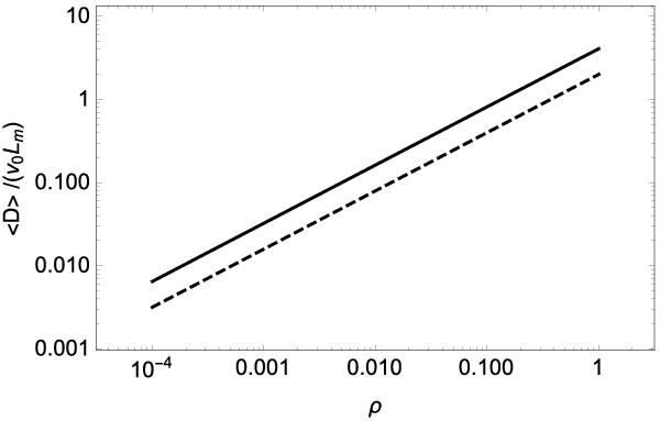
We also calculated the integral (28) numerically for different values of $\beta$, using the previously calculated function $\overline{F}(a)$. The result is shown in Figure 3. We see that the average diffusion coefficient weakly depends on $\beta$. So we consider only the Kolmogorov spectrum $\beta=1/3$ in what follows. From Figure 4 one can see that $\langle D\rangle\propto A$ for $A<1$. This is consistent with the analytical result (29) and gives the Bohm diffusion coefficient, $D\propto v_{0}r_{L}$.

For $A>1$, Figure 3 shows a slow growth of $\langle D(A)\rangle$. But as was shown in previous section, the diffusion coefficient for particles with $r_{L}>L_{0}$ increases proportionally to the square of the Larmor radius, i.e. $\langle D\rangle\propto A^{2}$.

The reason for the discrepancy is the following. For correct description of diffusion of particles with $r_{L}>L_{0}$, it is necessary to consider the particle motion on the scale much larger than $L_{0}$, which contradicts the expression (25). Hence the results calculated from (28) are applicable only for particles with $r_{L}<L_{0}$.

Adopting for the case $A>1$ the result (10), we approximately represent the diffusion coefficient for the Kolmogorov spectrum $\beta=1/3$ as

We note that two cases practically coincide at the point $A=1$. One can rewrite this formula in terms of $r_{L}$:

We see that diffusion of particles is primarily determined by their motion in a large-scale magnetic field and weakly depends on the spectrum of magnetic fluctuations. The index $\beta$ of the spectrum (25) enters only in the common factor in the function $\langle D(r_{L})\rangle$. Since the Larmor radius of the particle is proportional to its rigidity ${\cal R}$, $r_{L}={\cal R}/B_{LS}$, then for small rigidities the diffusion coefficient is proportional to the rigidity (energy), $D\propto{\cal R}$, and for large rigidities it proportional to the square of the rigidity, $D\propto{\cal R}^{2}$. The result (31) has a simple physical interpretation. The diffusion coefficient of particles is determined by their motion in a large-scale field (its amplitude is maximal for the spectral index $\beta>0$) and it is the increasing function of the Larmor radius.

References

- [1] Plotnikov I., Pelletier G., Lemoine M., Astron. Astrophys. 532, A68 (2011)
- [2] Jokipii J.R., ApJ 146, 480 (1966)
- [3] Shalchi A., Skoda T., Tautz R. C., Schlickeiser R., Astron. Astrophys. 507, 589 (2009)
- [4] Matthaeus W. H., Qin G., Bieber J. W., Zank G. P., ApJ 590, L53 (2003)
- [5] Dogiel V.A., Gurevich A.V., Istomin Ya.N., Zybin K.P., MNRAS 228, 843 (1987)
- [6] Zirakashvili V.N., Ptuskin V.S., Astropart. Phys. 39, 12 (2012)
- [7] Bohm D., Burhop E., The characteristics of electric discharges in magnetic fields, McGraw-Hill, New York (1949)
- [8] Casse F., Lemoine M., Pelletier G., Phys. Rev. D 65, 023002 (2002)
- [9] Snodin A.P., Shukurov A., Sarson G.R., Bushby P.J., Rodrigues L.F.S., MNRAS 457, 3975 (2016)
- [10] Hussein M., Shalchi A., ApJ 785, 31 (2014)
- [11] Beresnyak A., Yan H., Lazarian A., ApJ 728, 60 (2011)
- [12] Cohet R., Marcowith A., Astron. Astrophys. 588, A73 (2016)
- [13] Shukurov A.; Snodin A.P., Seta A., Bushby P.J.; Wood T.S., ApJ 839, L16 (2017)
- [14] Schekochihin A.A., Boldyrev S.A., Kulsrud R. M., ApJ 567, 828 (2002)
- [15] Istomin Ya.N., Kiselev A., MNRAS 436, 2774 (2013)
- [16] Berezinskii V. S., Bulanov S. V., Dogiel V. A., Ptuskin V. S., Astrophysics of cosmic rays, Edited by Ginzburg V.L., North-Holland, Amsterdam (1990)
- [17] Harrison E.R., Phys. Rev. D 1, 2726 (1970)
- [18] Zel’dovich Ya.B., MNRAS, 160, 1 (1972)