Error mitigation for short-depth quantum circuits
Abstract
Two schemes are presented that mitigate the effect of errors and decoherence in short-depth quantum circuits. The size of the circuits for which these techniques can be applied is limited by the rate at which the errors in the computation are introduced. Near-term applications of early quantum devices, such as quantum simulations, rely on accurate estimates of expectation values to become relevant. Decoherence and gate errors lead to wrong estimates of the expectation values of observables used to evaluate the noisy circuit. The two schemes we discuss are deliberately simple and don’t require additional qubit resources, so to be as practically relevant in current experiments as possible. The first method, extrapolation to the zero noise limit, subsequently cancels powers of the noise perturbations by an application of Richardson’s deferred approach to the limit. The second method cancels errors by resampling randomized circuits according to a quasi-probability distribution.
From the time quantum computation generated wide spread interest, the strongest objection to its viability was the sensitivity to errors and noise. In an early paper, William Unruh [1] found that the coupling to the environment sets an ultimate time and size limit for any quantum computation. This initially curbed the hopes that the full advantage of quantum computing could be harnessed, since it set limits on the scalability of any algorithm. This problem was, at least in theory, remedied with the advent of quantum error correction [2, 3, 4]. It was proven that if both the decoherence and the imprecision of gates could be reduced below a finite threshold value, then quantum computation could be performed indefinitely [5, 6]. Although it is the ultimate goal to reach this threshold in an experiment that is scalable to larger sizes, the overhead that is needed to implement a fully fault-tolerant gate set with current codes [7] seems prohibitively large [8, 9]. In turn, it is expected that in the near term the progress in quantum experiments will lead to devices with dynamics, which are beyond what can be simulated with a conventional computer. This leads to the question: what computational tasks could be accomplished with only limited, or no error correction?
The suggestions of near-term applications in such quantum devices mostly center around quantum simulations with short-depth circuit [10, 11, 12] and approximate optimization algorithms [13]. Furthermore, certain problems in material simulation may be tackled by hybrid quantum-classical algorithms [14]. In most such applications, the task can be abstracted to applying a short-depth quantum circuits to some simple initial state and then estimating the expectation value of some observable after the circuit has been applied. This estimation must be accurate enough to achieve a simulation precision comparable or exceeding that of classical algorithms. Yet, although the quantum system evolves coherently for the most part of the short-depth circuit, the effects of decoherence already become apparent as an error in the estimate of the observable. For the simulation to be of value, the effect of this error needs to be mitigated.
In this paper we introduce two techniques for quantum error mitigation that increase the quality of any such short-depth quantum simulations. We find that the accuracy of the expectation value can be increased significantly in the presence of noise. We are looking for error mitigation techniques that are as simple as possible and don’t require additional quantum resources. Both techniques require that some noise parameter taken together with system size and circuit depth can be considered a small number. The first scheme does not make any assumption about the noise model other than it being weak and constant in time. In comparison, the second scheme can tolerate stronger noise; however, it requires detailed knowledge of the noise model.
Extrapolation to the zero noise limit: It is our goal to estimate the expectation value of some quantum observable with respect to an evolved state after time that is subject to noise characterized by the parameter in the limit where . To achieve this, we apply Richardson’s deferred approach to the limit to cancel increasingly higher orders of [15].
Although gates are typically used to describe quantum circuits, for our analysis it is more convenient to consider the time-dependent Hamiltonian dynamics implementing the circuit. The time-dependent multi-qubit Hamiltonian is denoted by . It can be expanded into - qubit Pauli operators , where acts as a single-qubit Pauli matrix on site and trivially elsewhere. We allow for time-dependent coupling coefficients . The circuit is encoded as . The total evolution of the open system with initial state will be described by an equation of the following form:
| (1) |
for time . We do not specify the exact form of the generator but only require that it is invariant under time rescaling and independent from the parameters in . The noise term could be given as a Lindblad operator, or it could correspond to a Hamiltonian that couples to a bath to model non-Markovian dynamics. We ask that there is a parameter that indicates a weak action of the noise and that we can bound , where at most . The map is short-hand notation for the transformation of into the interaction frame generated by .
The expectation value of the observable is obtained from the final state as . The function can be expressed as a series in where the contribution with corresponds to the noise-free evolution. This can be seen by transforming the evolution into the interaction frame w.r.t and expanding the Born series, c.f. supp. mat. sec I. Starting from the noise-free expectation value , the expansion is given by
| (2) |
The are model-specific constants typically growing like . Here is the remainder of the expansion and can be bounded by by standard arguments. Since we assumed an extensive scaling of , such an expansion is only meaningful whenever is small. We are of course interested in ; however, we are faced with a small but finite parameter . Since we only have access to , our estimate of will be off by .
This estimate can be improved by Richardson’s deferred approach to the limit [15, 16]. To explain the idea, let us assume we can run the quantum circuit at different noise rates , with and obtain experimental estimates . Here the are appropriately rescaled values of the experimental noise rate . The estimate deviates from the actual expectation value due to experimental inaccuracies and finite sampling errors by an error . The estimate of can be significantly improved by considering the approximation , which is written as the linear combination
| (3) |
Here we require the coefficients to satisfy the linear system of equations [16].
| (4) |
The linear combination Eq. (3) will be an approximation to up to an error of order .
To obtain estimates at different noise rates , we use a rescaling trick. We run the same circuit times with rescaled parameters in . We follow the protocol:
- 1.
For
- (a)
choose a rescaling coefficient () and evolve with rescaled Hamiltonian , where
(5) for time .
- (b)
Estimate observable to obtain .
- (a)
- 2.
A rescaling of the equations shows that the state , which evolves under for time , satisfies , c.f. supp. mat. sec. II. Hence the estimates can be obtained from the runs rescaled according to the protocol.
If the protocol is performed for steps, the error between the exact expectation value and the estimator can be bounded by
| (6) |
Here and is the largest experimental error.
This follows from repeated application of the triangle inequality, c.f. supp. mat. sec. III. The equations (4) can be solved, and one finds that the coefficients , so that the constant can be evaluated. In the literature [16], several choices for progression of are common. The two most frequent series are exponential decrease (Bulirsch - Stoer) and harmonic decay. In our experiments we are actually increasing the noise rate starting from the optimal value, wheres it is common in the numerical literature to improve the small parameter. The result is, of course, the same.
Examples : To demonstrate this method we will consider three numerical examples. In all the examples the time evolution is given by a Hamiltonian that encodes a control problem. For a single drift step we evolve with a Hamiltonian , where the single qubit product unitary is chosen Haar-random, and the drift Hamiltonian is chosen with respect to a random graph and Gaussian distributed couplings .
The evolution is subject to three different noise models: first Fig 1(a), we evolve in the presence of depolarizing noise described by the sum of single qubit generators acting on all qubits. Second, Fig 1(b), we consider dephasing and amplitude damping noise on every qubit, where we have chosen a ratio of with a generator and . Third, Fig 1(c), we consider a highly non-Markovian setting, where each of the qubits is coupled to its own single-qubit bath via the Hamiltonian and the bath is prepared in the initial state . Then, after the evolution of each noisy circuit we measure a randomly chosen multi-qubit Pauli operator .
The graphs in Fig 1 show that with modest effort very high precisions can be obtained. In the low noise range the relative error can be reduced to . The precision is then essentially determined by the sampling error , which we have neglected in the plots.
Probabilistic error cancellation: Here we discuss a noise reduction scheme for quantum circuits subject to a Markovian noise. First let us state our assumptions on the noise model. A noisy -qubit device will be described by a basis set of noisy operations that can be implemented on this device. Each operation is a trace-preserving completely positive (TPCP) map on qubits that acts non-trivially only on a small subset of qubits, say at most two. For example, could be a noisy unitary gate applied to a specified pair of qubits or a noisy qubit initialization. We assume that noise in the system can be fully characterized such that the map is known for each . A circuit of length in the basis is a sequence of operations from . Let be a set of all length- circuits in the basis . A circuit implements a map . The expectation value of an observable on the final state produced by a noisy circuit is
For simplicity, we ignore errors in the initial state preparation and in the final measurement. Such errors can be accounted for by adding dummy noisy operations before each measurement and after each qubit initialization. Furthermore, we shall assume that is diagonal in the -basis and .
Below we show that under certain conditions the task of simulating an ideal quantum circuit can be reduced to estimating the expectation value for a suitable random ensemble of noisy quantum circuits . Moreover, the ideal and the noisy circuits act on the same number of qubits and have the same depth.
Let be a fixed basis set of ideal gates. Each gate is described by a unitary TPCP map on qubits that acts non-trivially on a small subset of qubits. An ideal length- circuit in the basis is a sequence of gates from . A circuit implements a map . Define an ideal expectation value
We consider a simulation task where the goal is to estimate with a specified precision .
The key idea of our scheme is to represent the ideal circuit as a quasi-probabilistic mixture of noisy ones. Let us say that a noisy basis simulates an ideal circuit with the overhead if there exists a probability distribution on the set of noisy circuits such that
| (7) |
for some coefficients . We also require that the distribution is sufficiently simple so that one can efficiently sample from . The coefficients must be efficiently computable. We shall refer to Eq. (41) as a quasi-probability representation (QPR) of the ideal circuit . Note that because and are trace-preserving. Quasi-probability distributions have been previously used to construct classical algorithms for simulation of quantum circuits [17, 18]. Our work can be viewed as an application of these methods to the problem of simulating ideal quantum circuits by noisy ones.
Substituting Eq. (41) into the definition of gives
| (8) |
Let be a random variable drawn from and be the final readout of the noisy circuit obtained by measuring each qubit of the final state in the -basis. Note that is an unbiased estimator of with the variance . Thus from Eq. (42) one infers that is an unbiased estimator of the ideal expectation value with the variance . We can now estimate with any desired precision by the Monte Carlo method. Define
| (9) |
and generate samples drawn from . By Hoeffding’s inequality, is approximated within error w.h.p. by a random variable
| (10) |
where is the final string of the noisy circuit . Computing the estimator requires runs of the noisy circuits, with each run producing a single readout string . Estimating with a precision in the absence of noise by Monte Carlo method would require approximately runs. Thus the quantity determines the simulation overhead (see Eq. (9)).
A systematic method of constructing QPRs with a small overhead is given in supp. mat. sec. IV. Here we illustrate the method using toy noise models usually studied in the quantum fault-tolerance theory: the depolarizing noise and the amplitude damping noise. For concreteness, we choose the ideal gate set as the standard Clifford+ basis.
Let be the depolarizing noise on qubits that returns the maximally mixed state with probability and does nothing with probability . Define a noisy version of a -qubit unitary gate as . The noisy basis is obtained by multiplying ideal gates on the left by arbitrary Pauli operators and adding the depolarizing noise. Thus is a set of operations , where is a -qubit ideal gate and is a Pauli TPCP map. The random ensemble of noisy circuits that simulates an ideal circuit is constructed in three steps: (1) Start from the ideal circuit, . (2) Modify by adding a Pauli after each single-qubit gate with probability . The gate is unchanged with probability . (3) Modify by adding a Pauli after each CNOT with probability . The CNOT is unchanged with probability . The resulting circuit is then implemented on a noisy device (which adds the depolarizing noise after each gate) and the final readout string is recorded. By generating samples of one can estimate from Eq. (10). The sign function is equal to , where is the number of Pauli operators added to the ideal circuit . As shown in supp. mat. sec. IV, the above defines a QPR of the ideal circuit with the overhead , where is the number of single-qubit gates and is the number of CNOTs in the ideal circuit. The method has been tested numerically for random noisy Clifford+ circuits, see Fig. 2.
A more interesting example is the noise described by the amplitude-damping channel that resets every qubit to its ground state with probability . A noisy version of a -qubit unitary gate is defined as . In contrast to the previous example, noisy unitary gates alone cannot simulate any ideal unitary gate since is not a unital map. To overcome this, we extend the noisy basis by adding noisy versions of single-qubit state preparations , where maps any input state to . Our scheme requires state preparations for single qubit states that can be performed at any time step (not only at the beginning). In supp. mat. sec. V we show how to construct a QPR of the ideal Clifford+ circuit with the overhead .
The examples considered above suggest that well-characterized noisy circuits can simulate ideal ones with overhead , where is the typical error rate and is a small constant. The value of can be determined by performing quantum process tomography [19] and finding the QPR for each ideal gate. Using Eq. (9), one can estimate the number of noisy circuit runs of length as . Assuming error rates in the range , it may be possible to simulate ideal circuits with gates.
Conclusions: Both error mitigation schemes require no additional quantum hardware such as ancilla or code qubits and work directly with the physical qubits. The zero-noise extrapolation requires sufficient control of the time evolution to implement the rescaled dynamics and hinges on the assumption of a large time-scale separation between the dominant noise and the controlled dynamics. For the probabilistic error cancellation a full characterization of the noisy computational operations is necessary. To obtain this to a precision of is challenging in practice. However, if one is willing to sacrifice optimality, a Pauli- or Clifford-twirling [20, 21] can be applied that converts any noise channel into a simple mixture of Pauli errors or depolarizing noise, making the characterization task much more manageable. A very recent independent paper by Li and Benjamin [22] discusses similar issues to those addressed here.
Acknowledgements: We thank Antonio Mezzacapo for insightful discussions, and we acknowledge support from the IBM Research Frontiers Institute
References
- [1] W. G. Unruh, Physical Review A 51, 992 (1995).
- [2] P. W. Shor, Physical review A 52, R2493 (1995).
- [3] A. M. Steane, Physical Review Letters 77, 793 (1996).
- [4] A. R. Calderbank and P. W. Shor, Physical Review A 54, 1098 (1996).
- [5] D. Aharonov and M. Ben-Or, in Proceedings of the twenty-ninth annual ACM symposium on Theory of computing (ACM, 1997) pp. 176–188.
- [6] A. Y. Kitaev, Russian Mathematical Surveys 52, 1191 (1997).
- [7] A. G. Fowler, M. Mariantoni, J. M. Martinis, and A. N. Cleland, Physical Review A 86, 032324 (2012).
- [8] N. C. Jones, R. Van Meter, A. G. Fowler, P. L. McMahon, J. Kim, T. D. Ladd, and Y. Yamamoto, Physical Review X 2, 031007 (2012).
- [9] S. J. Devitt, A. M. Stephens, W. J. Munro, and K. Nemoto, Nature communications 4 (2013).
- [10] A. Peruzzo, J. McClean, P. Shadbolt, M.-H. Yung, X.-Q. Zhou, P. J. Love, A. Aspuru-Guzik, and J. L. O?Brien, Nature communications 5 (2014).
- [11] J. R. McClean, J. Romero, R. Babbush, and A. Aspuru-Guzik, arXiv preprint arXiv:1509.04279 (2015).
- [12] D. Wecker, M. B. Hastings, and M. Troyer, Physical Review A 92, 042303 (2015).
- [13] E. Farhi, J. Goldstone, and S. Gutmann, arXiv preprint arXiv:1411.4028 (2014).
- [14] B. Bauer, D. Wecker, A. J. Millis, M. B. Hastings, and M. Troyer, arXiv preprint arXiv:1510.03859 (2015).
- [15] L. F. Richardson and J. A. Gaunt, Philosophical Transactions of the Royal Society of London. Series A, containing papers of a mathematical or physical character 226, 299 (1927).
- [16] A. Sidi, “Practical extrapolation methods: Theory and applications, volume 10 of cambridge monographs on applied and computational mathematics,” (2003).
- [17] H. Pashayan, J. J. Wallman, and S. D. Bartlett, Physical review letters 115, 070501 (2015).
- [18] N. Delfosse, P. A. Guerin, J. Bian, and R. Raussendorf, Physical Review X 5, 021003 (2015).
- [19] M. Mohseni, A. Rezakhani, and D. Lidar, Phys. Rev. A 77, 032322 (2008).
- [20] M. Silva, E. Magesan, D. W. Kribs, and J. Emerson, Physical Review A 78, 012347 (2008).
- [21] E. Magesan, J. M. Gambetta, and J. Emerson, Physical Review A 85, 042311 (2012).
- [22] Y. Li and S. C. Benjamin, arXiv preprint arXiv:1611.09301 (2016).
- [23] G. Lindblad, Communications in Mathematical Physics 48, 119 (1976).
- [24] H.-P. Breuer and F. Petruccione, The theory of open quantum systems (Oxford University Press on Demand, 2002).
- [25] C. Schneider, Numerische Mathematik 24, 177 (1975).
I Supplemental Material
Appendix A Reducing noise by Richardson extrapolation
In numerical analysis, Richardson extrapolation [15, 16] is a sequence acceleration method, used to improve the rate of convergence of a sequence. We use the same technique to extrapolate to the zero-noise limit in short-depth quantum circuits in the presence of noise. We assume that the noise process is constant in time and does not depend on the rescaling of the system Hamiltonian parameters. We consider various noise models in continuous time.
It is our goal to estimate the expectation value of some observable with respect to the evolved state . The actual computation is now encoded in the time-dependent Hamiltonian , and the full evolution is given by the equation
| (11) |
Here we have that
| (12) |
is some multi-qubit Pauli Hamiltonian with time-dependent coupling constant and Pauli operators . Starting from some initial state the system is evolved for some time . We consider different forms of noise . As the simplest form of noise, we assume a time-independent Lindblad operator [23] of the form
| (13) |
However, we can also imagine other forms of errors, such as
| (14) |
where is some Hamiltonian. This setting in useful when we want to consider more general, possibly non-Markovian noise models, or a noisy evolution derived from first principle [24]. One can make the assumption that the initial state is given by and give the most general form of an interaction Hamiltonian between system and bath, such as
| (15) |
Here we take the point of view that a small indicates a separation of time scales, and may be the initial state of the computation. We assume that , where the bath state is a steady state w.r.t the bath Hamiltonian . The observable we want to estimate is then only supported on the system degrees of freedom.
We assume that is the state we obtain after the noisy evolution for time . From this state we can estimate the expectation value of the observable by various methods. Typically we will sample the expectation value
| (16) |
so that an additional sampling error is introduced, and we obtain from out measurement the statistic . The error can assumed to be asymptotically Gaussian since one typically repeats the experiment times and the i.i.d hypothesis holds.
A.1 I Series expansion in the noise parameter
We now show that the function can be expressed as a series in where the contribution with corresponds to the noise-free evolution. We also provide a bound on the error term. To this end, we transform into the interaction picture of . We define , where defines the time order expansion. We define the interaction picture through
| (17) |
where now the generator has become time-dependent. The evolution equation in the interaction picture now reads
| (18) |
Recall that every first-order differential equation can be reformulated as an integral equation
| (19) |
This equation can be recursively solved to increasing order in so that
| (20) | |||||
Recall that . Furthermore, we can conjugate the full expression on both sides with the unitary . Let us for notational convenience define as the resulting state after evolution with noise rate . We observe that , whereas , so that we obtain the expression in the Schrödinger picture as
| (21) | |||||
The expectation value for the observable can immediately be expanded in a series with parameter of the form
| (22) |
where the constants and the remainder are obtained by pairing the integrals with the trace and corresponds to the noise-free evolution to which we seek to extrapolate. We read off that
| (23) |
as well as
| (24) |
We can bound by a simple application of Cauchy’s mean value theorem and Hölder’s inequality. We observe by first applying the midpoint Theorem that there exist so that
| (25) |
We can then of course immediately bound the inner product
| (26) |
by a direct application of Hölder’s inequality. Note that all Schatten norms are unitarily invariant, so when the map is bounded, we can apply the subsequent operator norm inequalities
| (27) |
It is safe to assume that a Lindblad operator acting on a finite dimensional system, such as a collection of qubits, is bounded. However, we also consider the case of a first-principle noise model that can even be non-Markvoian. In this setting the operator is expected to couple to an arbitrary large bath and may contain unbounded operators, such as bosonic operators. In such a setting an upper bound in terms of an operator norm of is a moot point. Yet, in this case we can transform the evolution into the Heisenberg picture , for the observable , and look at the equations for instead. The almost identical analysis as performed above can be carried through, but this time we can obtain a bound on
| (28) |
We obtain almost the same type of bound from Hölder’s inequality since for contractive evolutions, where the sole difference is now that only depends on the initial state. Since we now consider the action of the operators in on a well-behaved initial state , we can assume that is a reasonable bound. In either case, we will now write for the bound on from now on:
| (29) |
The coefficients can be bounded in a similar fashion. Note that, if we assume that noise acts locally on each qubit, such as for instance, when the dissipator corresponds to single-qubit depolarizing noise, so that . We have that is extensive in the system size. A similar argument holds for the case when the individual qubits couple to a bath. From this we can deduce that for local noise we typically find as mentioned in the main text, and that .
It is also worthwhile to point out the following observation. For different types of error terms it may happen that not all powers of are present in the expansion. It is conceivable that some system bath interactions could lead to an expansion in only even powers of . If this occurs, the Richardson extrapolation method is particularly efficient, since a higher order of precision can be obtained with fewer values of .
A.2 II Experimental rescaling of the noise parameter
In order to apply Richardson extrapolation, we have to be able to evaluate for different values of . In an actual experiment, we can’t directly control the parameter : however, we may control the evolution . To this end, we introduce a rescaling. We redefine
| (30) |
We claim that this rescaling maps if the noise operator does not depend on the Hamiltonian couplings and is constant in time. This rescaled density matrix then leads to a new evaluation of the expectation value. To see that the rescaling has the desired effect, we again make use of the integral representation of , for which we can write now in the Schrödinger picture
| (31) |
We can now choose a re-parametrization of the evolution and an increased runtime , and write
| (32) |
with . If we now substitute the integration variable according to , we have that , which leads to
| (33) | |||||
Hence, rescaling the evolution according to equation (30) leads to an effective rescaling of the dissipative rate . This can be done for any constant dissipator and allows the experimenter to evaluate for different values of so that we can apply the Richardson extrapolation procedure.
Note that for different experimental circumstances, other rescaling methods of the parameter may actually be easier to implement. For example, in an optical experiment that is plagued by photon loss, it may be suitable to consider different methods of directly changing the photon loss rate. The only requirement is that the modification of can be performed sufficiently accurately so the extrapolation can be performed.
A.3 III Error bounds on the noise-free estimator
Let us now show that the protocol leads to the desired error bound on the estimated expectation value as claimed in the main text. Recall that we first choose a set of rescaling parameters , to evolve with respect to the rescaled Hamiltonian for time . As discussed in the previous section, this evolution leads to a state , c.f. Eq. (33) as was discussed in section II. If we now measure the observable on these states we obtain for the estimates . Recall the set of equations for defined in [25] and given in the main text, which requires for the that
| (34) |
Now we observe that estimators can be expressed as
| (35) |
due to the expansion (22) discussed in section I. Recall now the definition of our improved estimator as given in the main text, , for which then
| (36) | |||||
Recall the equations for from which we can then infer after the application of the triangle inequality
| (37) |
After the application of the bound and the observation that , we can bound the difference with and obtain the final bound
| (38) |
with .
In the Richardson extrapolation literature [16], two types of sequences are considered frequently. In the Bulirsch - Stoer series the rescalings are chosen so that constitutes an exponential series, which is typically chosen at base ; but harmonic series have also been frequently applied, e.g. for parameters one can choose . Note that in our experiments we are actually increasing the noise rate starting from the optimal value, whereas it is common in the numerical literature to improve the small parameter, so that . The result here is of course the same, and just corresponds to a reordering of the labels when is finite. For both of the aforementioned cases, a bound on has been derived. One is mostly interested in the asymptotic behavior of as in order to analyze the numerical stability of the method. In current experiments we only expect to go to third or forth order, making the stability analysis less relevant.
Appendix B Probabilistic error cancellation by resampling
The key idea of our scheme is to represent the ideal circuit as a quasi-probabilistic mixture of noisy ones. Central to this approach is the quasi probability representation (QPR) of the noise-free circuit . We note that quasi-probability distributions have been previously used to construct classical algorithms for simulation of quantum circuits [17, 18]. Our work can be viewed as an application of these methods to the problem of simulating ideal quantum circuits by noisy ones.
The general approach to constructing a QPR for a quantum circuit is the following: Suppose you are given a set of noisy operations that can be implemented on a noisy -qubit device. We assume that we can perform gate tomography [19] to specify the gates with an accuracy that is comparable to the desired accuracy of the ideal circuit. These noisy operations are noisy versions of ideal quantum gates and are assumed to form a full basis of TPCP operations, i.e. an element is always of the form
| (39) |
A crucial condition is that the set of noisy operators constitutes a basis in the space of TPCP operations that is sufficiently large, so that any ideal, unitary gate can be expressed as a linear combination of noisy gates in . Hence, there have to be coefficients , and noisy operations in so that we can write for any ideal gate in the circuit
| (40) |
This linear expansion of can then be cast into the form of a quasi-probability representation.
On real quantum devices we can only apply the noisy operations . We say that a circuit of length in the basis is a sequence of operations from . Such a circuit, c.f. Fig 3(b), indexed by implements a noisy map .
The expectation value of an observable on the final state produced by a noisy circuit is
For simplicity, we ignore errors in the initial state preparation and in the final measurement. Such errors can be accounted for by adding dummy noisy operations before each measurement and after each qubit initialization. Furthermore, we shall assume that is diagonal in the -basis and .
The task of simulating an ideal quantum circuit , c.f. Fig. 3(a), of ideal gates , can be reduced to estimating the expectation values for a suitable random ensemble of noisy quantum circuits . That is, we can obtain estimates for the ideal expectation values
after the application of the circuit by estimating noisy circuit outputs. Moreover, the ideal and the noisy circuits act on the same number of qubits and have the same length.
We say that the noisy basis simulates an ideal circuit if there exists a probability distribution on the set of noisy circuits such that
| (41) |
for some coefficients . We require that the distribution is sufficiently simple so that one can efficiently sample from . The coefficients must be efficiently computable.
We can see that the estimates of the noisy circuit are related to the ideal circuit probability by substituting Eq. (41) into the definition of . This gives
| (42) |
The construction of QPRs with optimal overhead of general operation-dependent noise is an interesting open problem. A preliminary analysis shows that a noisy basis that includes noisy versions of all single-qubit and two-qubit Clifford gates, -gates, and noisy qubit initializations in the basis can simulate any ideal gate from the Clifford+ gate set with the overhead , provided that each noisy operation is -close to its ideal analogue. Unfortunately, the constant coefficient in this upper bound is far too large to have any practical implications.
Furthermore, the full Clifford group on two-qubits contains gates. It may not be feasible to perform process tomography for each of those gates. We shall see that for certain noise models, such as the amplitude damping noise, QPRs can be constructed only if the noisy basis includes some qubit initialization maps. In particular, noisy circuits that appear in Eq. (41) may apply qubit initializations at intermediate time steps, even though the ideal circuit initializes all the qubits at the very first step. All QPRs constructed below preserve the circuit depth. That is, if the ideal circuit has depth then all noisy circuits in Eq. (41) have depth at most .
B.1 IV Minimal overhead decomposition of noise free circuit
Let us discuss how to construct QPRs with a small overhead. For concreteness, we choose the ideal gate set as the Clifford+ basis. It includes the identity gate , the Hadamard gate , phase-shift gates and , and the CNOT. For technical reasons, we shall assume that each CNOT is followed by single-qubit gates (that could be identity gates). We shall consider toy noise models usually studied in the quantum fault-tolerance theory: the depolarizing noise and the amplitude damping noise.
First let us describe product QPRs that can be constructed independently for each gate in the ideal circuit. Consider a fixed ideal gate . Let be the list of all noisy operations whose support is contained in the support of . Consider the following linear program with real variables .
| (43) |
| (44) |
Suppose is the optimal solution of the program. Note that for all since otherwise the objective function can be decreased. Define , , and . Then
| (45) |
which is a gate-wise version of the QPR Eq. (41). We shall say that a noisy basis simulates a gate with the overhead if the linear program Eqs. (43,44) has a feasible solution with value . A product QPR of the ideal circuit is defined as a product of all gate-wise QPRs Eq. (45). It gives , and . The assumption that all noisy operations in Eq. (44) act non-trivially only within the support of allows one to restrict Eq. (44) to operations acting on at most two qubits. Such operations can be represented by real matrices of size by computing matrix elements of and in the Pauli basis. Thus the program Eqs. (43,44) can be solved in time . Since the ideal gate set has size , product QPRs can be computed in time . Furthermore, if two ideal gates have disjoint supports, then the gate-wise QPRs defined in Eq. (45) have disjoint supports. Thus product QPRs preserve the circuit depth.
B.2 V Depolarizing noise cancellation and numerical results
Let us illustrate the construction of product QPRs using the depolarizing noise as an example. Let be the -depolarizing channel on qubits that returns the maximally mixed state with probability and does nothing with probability . Define a noisy version of a -qubit unitary gate as . Define a noisy basis by multiplying ideal gates on the left by arbitrary Pauli operators and adding the depolarizing noise. Thus is a set of operations , where is a -qubit ideal gate and is a Pauli TPCP map. A Pauli map corresponding to a Pauli operator is defined by . Here . We claim that simulates ideal single-qubit gates with the overhead and simulates CNOTs with the overhead .
Indeed, suppose is a single-qubit gate. Let us look for a solution of Eq. (44) in the form , where . Then Eq. (44) is equivalent to
One can easily check that the optimal solution minimizing is and for . Therefore . The CNOT is simulated in a similar fashion by representing as a linear combination of two-qubit Pauli maps. The random ensemble of noisy circuits that simulates an ideal circuit is constructed in three steps:
- 1.
Start from the ideal circuit, .
- 2.
Modify by adding a Pauli after each single-qubit gate with probability . The gate is unchanged with probability .
- 3.
Modify by adding a Pauli after each CNOT with probability . The CNOT is unchanged with probability .
The resulting circuit is then implemented on a noisy device (which adds the depolarizing noise after each gate) and the final readout string is recorded. By generating samples of one can estimate using Eq. (10) of the main text. The sign function is equal to , where is the number of Pauli operators added to the ideal circuit to obtain .
B.2.1 Numerical simulations
The error cancellation method was tested numerically for small Clifford+ circuits subject to the depolarizing noise. We choose the ideal circuit as a composition of alternating layers of gates, with each layer being either a tensor product of single-qubit gates (for odd layers) or a tensor product of CNOTs (for even layers). The resulting circuit has depth . Simulations were performed for random circuits as above with the initial state . Each single-qubit gate was picked randomly from the set . Control and target qubits for each CNOT were picked at random.
For each ideal circuit we choose the observable as a projector onto the subset of basis states whose probability in the final state of is above the median value. In other words,
By construction, for any circuit . Furthermore, we observed that is well separated from for most of the circuits see Fig. 4.
Recall that we define a noisy version of a -qubit unitary gate as , where
is the depolarizing channel on qubits. Noise was added after all gates including the identity gates. In this case the total simulation overhead depends only on the number of qubits and the circuit depth, namely
Consider a fixed ideal circuit and let , be the random ensemble of noisy circuits obtained from by inserting random Pauli operators and adding noise as described in the main text. Instead of using the estimate Eq. (10) of the main text for the ideal output probability we opted for a slightly optimized estimate. It is defined by dividing the total budget of runs into groups such that the -th group contains runs
Define a random variable
| (46) |
where are independent samples drawn from the distribution and are readout strings obtained by measuring each qubit of the final state in the -basis. We prepare a fresh copy of the final state to generate each string . Thus computing requires runs of the noisy circuits with each run producing a single readout string. One can easily check that is an unbiased estimator of for any choice of . Our goal is to choose that minimize the variance of for a fixed . One can easily check that the optimal choice is
where . In order to choose optimal values of , one has to run each circuit at least a few times, which gives a rough estimate of and thus . Numerical simulations were performed for the following parameters:
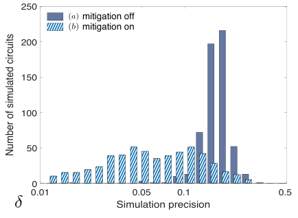
Our results are presented on the left panel of Figure 5. For each of ideal circuits generated at random we computed a simulation precision where is the estimate defined in Eq. (46). The plot on Figure 5, left, shows distribution of the ideal circuits according to their simulation precision . The median value of is approximately . This is consistent with the estimate
We also computed a simulation precision that one would obtain by running the circuit directly on a noisy device without error cancellation, see the right panel of Figure 5. It is defined as . For each circuit the output probability was estimated using circuit runs. Thus the simulations presented on the left and the right panels of Figure 5 have access to exactly the same resources. The median value of is approximately . We conclude that error cancellation significantly improves the simulation precision.
B.3 VI Quasi-probability representation for amplitude-damping noise
A more interesting example is the noise described by the amplitude-damping channel , where
A noisy version of a -qubit unitary gate is defined as . In contrast to the previous example, noisy unitary gates alone cannot simulate any ideal unitary gate. Indeed, assume the contrary. Suppose is a single-qubit gate that has a QPR Eq. (45) with for some unitary maps . Rewrite Eq. (45) as
Since the maps are unital, we infer that and are unital which is false. Thus Eq. (45) has no solutions.
To overcome this problem we shall extend the noisy basis by adding state preparations. Also we shall employ non-product QPRs. Given a single-qubit state , define a state preparation map
| (47) |
Let be the -gate considered as a TPCP map. Define a noisy basis that includes noisy state preparations with , noisy single-qubit gates , for each ideal single-qubit gate , and noisy two-qubit gates
where are the control and the target qubits of a CNOT gate . Here the subscripts indicate qubits acted upon by each map. We claim that this noisy basis simulates any ideal Clifford+ circuit with the overhead
| (48) |
where is the number of -qubit gates in . The corresponding QPR Eq. (41) preserves the circuit depth, although it does not have a simple product form as above.
Indeed, consider a single-qubit gate . Let us look for a solution of Eq. (44) with and
Note that since . Furthermore, since , one can rewrite Eq. (44) as
| (49) |
One can easily check that the optimal solution minimizing is
Therefore, simulates with the overhead , where is defined in Eq. (48).
Next consider the CNOT gate . Consider a decomposition of obtained by applying Eq. (49) twice. Multiplying this decomposition on the right by and on the left by one obtains
| (50) |
where is a valid noisy operation and is either identity or a state preparation map applied to the control and/or target qubits. Here we noted that . Although might not be a valid noisy operation from , we may merge with the next gate applied after the CNOT. Indeed, by assumption, each CNOT in the ideal circuit is followed by some single-qubit gates and applied to the control and the target qubits. The gates can be absorbed into since they act trivially on the state . The only non-trivial case is when is merged with the Hadamard gate. In this case the latter is replaced by the state preparation .
Since can now appear in the ideal circuit, we must be able to use noisy operations from to simulate . Let us look for a solution of Eq. (44) with in the form
| (51) |
Note that the righthand side of Eq. (51) contains only noisy operations from . One can rewrite Eq. (51) as
The optimal solution minimizing is
Therefore simulates the ideal state preparation with the overhead , where is defined in Eq. (48).
A QPR of the ideal circuit with the overhead Eq. (48) is constructed in two steps. First, one applies the decomposition Eq. (50) to each CNOT of and merges state preparation maps that appear in (if any) with the single-qubit gates of following the CNOT. Now all CNOT gates are replaced by noisy gates from . The rest of the circuit consists of single-qubit gates and state preparations . At the second step, each of these ideal operations is replaced by its QPR constructed above. Note that each CNOT contributes to the total overhead , see Eq. (50). Each single-qubit gate or a state preparation contributes at most to the total overhead. This proves Eq. (48).