Approximation by $C^{1}$ Splines on Piecewise Conic Domains

Spaces of piecewise polynomials defined on domains bounded by piecewise algebraic curves and vanishing on parts of the boundary can be used in the Finite Element Method as an alternative to the classical mapped curved elements [7, 11]. Since implicit algebraic curves and surfaces provide a well-known modeling tool in CAGD [1], these methods are inherently isogeometric in the sense of [14]. Moreover, this approach does not suffer from the usual difficulties of building a globally $C^{1}$ or smoother space of functions on curved domains (see (4, Section 4.7)) shared by the classical curved finite elements and the B-spline-based isogeometric analysis.

In particular, a space of $C^{1}$ piecewise polynomials on domains enclosed by piecewise conic sections has been studied in [11] and applied to the numerical solution of fully nonlinear elliptic equations. These piecewise polynomials are quintic on the interior triangles of a triangulation of the domain, and sextics on the boundary triangles (pie-shaped triangles with one side represented by a conic section as well as those triangles that share with them an interior edge with one endpoint on the boundary) and generalize the well-know Argyris finite element. Although local bases for these spaces have been constructed in [11] and numerical examples demonstrated the convergence orders expected from a piecewise quintic finite element, no error bounds have been provided.

In this paper we study the approximation properties of the spaces introduced in [11]. We define a Hermite-type interpolation operator and prove an error bound that shows the convergence order $\mathcal{O}(h^{6})$ of the residual in $L_{2}$-norm, and order $\mathcal{O}(h^{6-k})$ in Sobolev spaces $H^{k}(\Omega)$. This extends the techniques used in [7] for $C^{0}$ splines to Hermite interpolation.

The paper is organized as follows. We introduce in Section 2 the spaces $\mathbb{S}^{1,2}_{d,0}(\triangle)$ of $C^{1}$ piecewise polynomials on domains bounded by a number of conic sections, with homogeneous boundary conditions, define in Section 3 our interpolation operator in the case $d=5$, and investigate in Section 4 its approximation error for functions in Sobolev spaces $H^{m}(\Omega)$, $m=5,6$, vanishing on the boundary.

We make the same assumptions on the domain and its triangulation as in [7, 11], as outlined below.

Let $\Omega\subset\mathbb{R}^{2}$ be a bounded curvilinear polygonal domain with $\Gamma=\partial\Omega=\bigcup_{j=1}^{n}\overline{\Gamma}_{j}$, where each $\Gamma_{j}$ is an open arc of an algebraic curve of at most second order ( i.e., either a straight line or a conic). For simplicity we assume that $\Omega$ is simply connected, so that its boundary $\Gamma$ is a closed curve without self-intersections. Let $Z=\{z_{1},\ldots,z_{n}\}$ be the set of the endpoints of all arcs numbered counter-clockwise such that $z_{j},z_{j+1}$ are the endpoints of $\Gamma_{j}$, $j=1,\ldots,n$, with $z_{j+n}=z_{j}$. Furthermore, for each $j$ we denote by $\omega_{j}$ the internal angle between the tangents $\tau^{+}_{j}$ and $\tau^{-}_{j}$ to $\Gamma_{j}$ and $\Gamma_{j-1}$, respectively, at $z_{j}$. We assume that $\omega_{j}\in(0,2\pi)$ for all $j$. Hence $\Omega$ is a Lipschitz domain.

Let $\triangle$ be a triangulation of $\Omega$,  i.e., a subdivision of $\Omega$ into triangles, where each triangle $T\in\triangle$ has at most one edge replaced with a curved segment of the boundary $\partial\Omega$, and the intersection of any pair of the triangles is either a common vertex or a common (straight) edge if it is non-empty. The triangles with a curved edge are said to be pie-shaped. Any triangle $T\in\triangle$ that shares at least one edge with a pie-shaped triangle is called a buffer triangle, and the remaining triangles are ordinary. We denote by $\triangle_{0}$, $\triangle_{B}$ and $\triangle_{P}$ the sets of all ordinary, buffer and pie-shaped triangles of $\triangle$, respectively, such that $\triangle=\triangle_{0}\cup\triangle_{B}\cup\triangle_{P}$ is a disjoint union, see Figure 1. Let $V,E,V_{I},E_{I},V_{\partial},E_{\partial}$ denote the set of all vertices, all edges, interior vertices, interior edges, boundary vertices and boundary edges, respectively.

For each $j=1,\ldots,n$, let $q_{j}\in\mathbb{P}_{2}$ be a polynomial such that $\Gamma_{j}\subset\{x\in\mathbb{R}^{2}\,:\;q_{j}(x)=0\}$, where $\mathbb{P}_{d}$ denotes the space of all bivariate polynomials of total degree at most $d$. By changing the sign of $q_{j}$ if needed, we ensure that $q_{j}(x)$ is positive for points in $\Omega$ near the boundary segment $\Gamma_{j}$. For simplicity we assume in this paper that all boundary segments $\Gamma_{j}$ are curved. Hence each $q_{j}$ is an irreducible quadratic polynomial and

$$\nabla q_{j}(x)\neq 0\quad\text{if}\quad x\in\Gamma_{j}.$$

(1)

We assume that $\triangle$ satisfies the following conditions:

• (A)

  $Z=\{z_{1},\ldots,z_{n}\}\subset V_{\partial}$.

• (B)

  No interior edge has both endpoints on the boundary.

• (C)

  No pair of pie-shaped triangles shares an edge.

• (D)

  Every $T\in\triangle_{P}$ is star-shaped with respect to its interior vertex $v$.

• (E)

  For any $T\in\triangle_{P}$ with its curved side on $\Gamma_{j}$, $q_{j}(z)>0$ for all $z\in T\setminus\Gamma_{j}$.

• (F)

  No pair of buffer triangles shares an edge.

It can be easily seen that (B) and (C) are achievable by a slight modification of a given triangulation, while (D) and (E) hold for sufficiently fine triangulations. The assumption (F) is made for the sake of simplicity of the analysis. Note that the triangulation shown in Figure 1 does not satisfy (F).

For any $T\in\triangle$, let $h_{T}$ denote the diameter of $T$, and let $\rho_{T}$ be the radius of the disk $B_{T}$ inscribed in $T$ if $T\in\triangle_{0}\cup\triangle_{B}$ or in $T\cap T^{*}$ if $T\in\triangle_{P}$, where $T^{\ast}$ denotes the triangle obtained by joining the boundary vertices of $T$ by a straight line, see Figure 2. Note that every triangle $T\in\triangle$ is star-shaped with respect to $B_{T}$. In particular, for $T\in\triangle_{P}$ this follows from Condition (D) and the fact that the conics do not possess inflection points.

We define the shape regularity constant of $\triangle$ by

$$R=\max_{T\in\triangle}\frac{h_{T}}{\rho_{T}}.$$

(2)

For any $d\geq 1$ we set

	$\displaystyle\mathbb{S}^{1}_{d}(\triangle)$	$\displaystyle:=\{s\in C^{1}(\Omega)\,:\;s|_{T}\in\mathbb{P}_{d},\;T\in\triangle_{0},\;\text{and}\;s|_{T}\in\mathbb{P}_{d+1},\;T\in\triangle_{P}\cup\triangle_{B}\},$
	$\displaystyle\mathbb{S}^{1,2}_{d,I}(\triangle)$	$\displaystyle:=\{s\in\mathbb{S}^{1}_{d}(\triangle)\,:\;s\text{ is twice differentiable at any }v\in V_{I}\},$
	$\displaystyle\mathbb{S}^{1,2}_{d,0}(\triangle)$	$\displaystyle:=\{s\in\mathbb{S}^{1,2}_{d,I}(\triangle)\,:\;s|_{\Gamma}=0\}.$

We refer to [11] for the construction of a local basis for the space $\mathbb{S}^{1,2}_{5,0}(\triangle)$ and its applications in the Finite Element Method.

Our goal is to obtain an error bound for the approximation of functions vanishing on the boundary by splines in $\mathbb{S}^{1,2}_{5,0}(\triangle)$. This is done through the construction of an interpolation operator of Hermite type. Note that a method of stable splitting was employed in [6, 9, 10] to estimate the approximation power of $C^{1}$ splines vanishing on the boundary of a polygonal domain. $C^{1}$ finite element spaces with a stable splitting are also required in Böhmer’s proofs of the error bounds for his method of numerical solution of fully nonlinear elliptic equations [2]. A stable splitting of the space $\mathbb{S}^{1,2}_{5,I}(\triangle)$ will be obtained if a stable local basis for a stable complement of $\mathbb{S}^{1,2}_{5,0}(\triangle)$ in $\mathbb{S}^{1,2}_{5,I}(\triangle)$ is constructed, which we leave to a future work.

We denote by $\partial^{\alpha}f$, $\alpha\in\mathbb{Z}^{2}_{+}$, the partial derivatives of $f$ and consider the usual Sobolev spaces $H^{m}(\Omega)$ with the seminorm and norm defined by

$$|f|_{H^{m}(\Omega)}^{2}=\sum_{|\alpha|=m}\|\partial^{\alpha}f\|_{L^{2}(\Omega)}^{2},\quad\|f\|_{H^{m}(\Omega)}^{2}=\sum_{k=0}^{m}|f|_{H^{k}(\Omega)}^{2}\quad(H^{0}(\Omega)=L^{2}(\Omega)),$$

where $|\alpha|:=\alpha_{1}+\alpha_{2}$. We set $H^{1}_{0}(\Omega)=\{f\in H^{1}(\Omega):f|_{\partial\Omega}=0\}$.

In this section we construct an interpolation operator $I_{\triangle}:H^{5}(\Omega)\cap H^{1}_{0}(\Omega)\to\mathbb{S}^{1,2}_{5,0}(\triangle)$ and estimate its error for the functions in $H^{m}(\Omega)\cap H^{1}_{0}(\Omega)$, $m=5,6$, in the next section.

As in [7] we choose domains $\Omega_{j}\subset\Omega$, $j=1,\ldots,n$, with Lipschitz boundary such that

• (a)

  $\partial\Omega_{j}\cap\partial\Omega=\Gamma_{j}$,

• (b)

  $\partial\Omega_{j}\setminus\partial\Omega$ is composed of a finite number of straight line segments,

• (c)

  $q_{j}(x)>0$ for all $x\in\overline{\Omega}_{j}\setminus\Gamma_{j}$, and

• (d)

  $\Omega_{j}\cap\Omega_{k}=\emptyset$ for all $j\neq k$.

In addition we assume that the triangulation $\triangle$ is such that

• (e)

  $\overline{\Omega}_{j}$ contains every triangle $T\in\triangle_{P}$ whose curved edge is part of $\Gamma_{j}$,

and that $q_{j}$ satisfy (without loss of generality)

• (f)

  $\displaystyle\max_{x\in\overline{\Omega}_{j}}\|\nabla q_{j}(x)\|_{2}\leq 1\text{ and }\|\nabla^{2}q_{j}\|_{2}\leq 1,\;\text{for all }j=1,\ldots,n$,

where $\nabla^{2}q_{j}$ denotes the (constant) Hessian matrix of $q_{j}$.

Note that (e) will hold with the same set $\{\Omega_{j}:j=1,\ldots,n\}$ for any triangulations obtained by subdividing the triangles of $\triangle$.

The following lemma can be shown following the lines of the proof of (13, Theorem 6.1), see also (7, Theorem 3.1).

Given a a unit vector $\tau=(\tau_{x},\tau_{y})$ in the plane, we denote by $D_{\tau}$ the directional derivative operator in the direction of $\tau$ in the plane, so that

$$D_{\tau}f:=\tau_{x}D_{x}f+\tau_{y}D_{y}f,\quad D_{x}f:=\partial f/\partial x,\quad D_{y}f:=\partial{f}/\partial{y}.$$

Given $f\in C^{\alpha+\beta}(\triangle),~\alpha,\beta\geq 0$, any number

$$\eta f=D^{\alpha}_{\tau_{1}}D^{\beta}_{\tau_{2}}(f|_{T})(z),$$

where $T\in\triangle,~z\in T$, and $\tau_{1},\tau_{2}$ are some unit vectors in the plane, is said to be a nodal value of $f$, and the linear functional $\eta:C^{\alpha+\beta}(\triangle)\rightarrow\mathbb{R}$ is a nodal functional, with $d(\eta):=\alpha+\beta$ being the degree of $\eta$.

For some special choices of $z,\tau_{1},\tau_{2}$, we use the following notation:

• •

  If $v$ is a vertex of $\triangle$ and $e$ is an edge attached to $v$, we set

  $$D_{e}^{\alpha}f(v):=D_{\tau}^{\alpha}(f|_{T})(v),\quad\alpha\geq 1,$$

  where $\tau$ is the unit vector in the direction of $e$ away from $v$, and $T\in\triangle$ is one of the triangles with edge $e$.

• •

  If $v$ is a vertex of $\triangle$ and $e_{1},e_{2}$ are two consecutive edges attached to $v$, we set

  $$D^{\alpha}_{e_{1}}D^{\beta}_{e_{2}}f(v):=D^{\alpha}_{\tau_{1}}D^{\beta}_{\tau_{2}}(f|_{T})(v),\quad\alpha,\beta\geq 1,$$

  where $T\in\triangle$ is the triangle with vertex $v$ and edges $e_{1},e_{2}$, and $\tau_{i}$ is the unit vector in the $e_{i}$ direction away from $v$.

• •

  For every edge $e$ of the triangulation $\triangle$ we choose a unit vector $\tau^{\bot}$ (one of two possible) orthogonal to $e$ and set

  $$D^{\alpha}_{e^{\bot}}f(z):=D^{\alpha}_{\tau^{\bot}}f(z),\quad z\in e,\quad\alpha\geq 1,$$

  provided $f\in C^{\alpha}(z)$.

On every edge $e$ of $\triangle$, with vertices $v^{\prime}$ and $v^{\prime\prime}$, we define three points on $e$ by

$$z_{e}^{j}:=v^{\prime}+\frac{j}{4}(v^{\prime\prime}-v^{\prime}),\quad j=1,2,3.$$

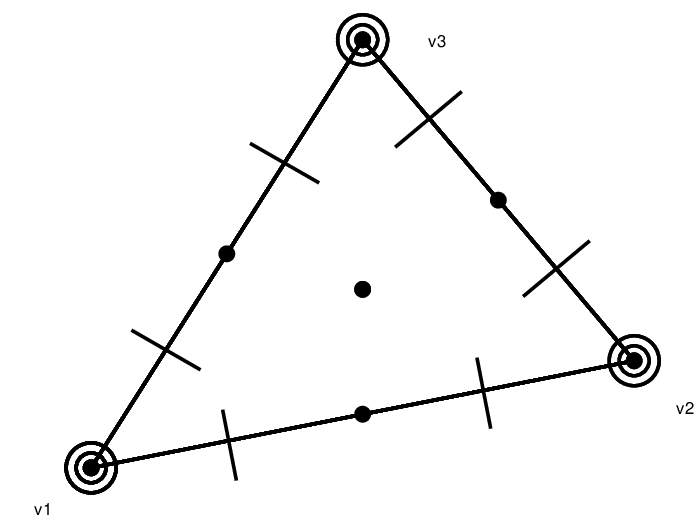
For every triangle $T\in\triangle_{0}$ with vertices $v_{1},v_{2},v_{3}$ and edges $e_{1},e_{2},e_{3}$, we define $\mathcal{N}_{T}^{0}$ to be the set of nodal functionals corresponding to the nodal values

$$D_{x}^{\alpha}D_{y}^{\beta}f(v_{i}),\quad 0\leq\alpha+\beta\leq 2,\quad i=1,2,3,$$

$$D_{e_{i}^{\bot}}f(z_{e_{i}}^{2}),\quad i=1,2,3,$$

see Figure 3 (left), where the nodal functionals are depicted in the usual way by dots, segments and circles as for example in [5].

Let $T\in\triangle_{P}$. We define $\mathcal{N}_{T}^{P}$ to be the set of nodal functionals corresponding to the nodal values

$$D_{x}^{\alpha}D_{y}^{\beta}f(v_{1}),\quad 0\leq\alpha+\beta\leq 2,$$

$$D^{\alpha}_{x}D^{\beta}_{y}f(v_{i}),\quad 0\leq\alpha+\beta\leq 1,\quad i=2,3,$$

$$D_{x}^{\alpha}D_{y}^{\beta}f(c_{T}),\quad 0\leq\alpha+\beta\leq 1,$$

where $v_{1}$ the interior vertex of $T$, $v_{2},v_{3}$ are boundary vertices, and $c_{T}$ is the center of the disk $B_{T}$, see Figure 4.

Let $T\in\triangle_{B}$ with vertices $v_{1},v_{2},v_{3}$. We define $\mathcal{N}_{T}^{B,1}$ to be the set of nodal functionals corresponding to the nodal value

$$f(c_{T}),\quad c_{T}:=(v_{1}+v_{2}+v_{3})/3.$$

Also we define $\mathcal{N}_{T}^{B,2}$ to be the set of nodal functionals corresponding to the nodal values

$$f(z_{e_{i}}^{2}),\quad i=1,2,3,$$

$$D_{x}^{\alpha}D_{y}^{\beta}f(v_{i}),\quad 0\leq\alpha+\beta\leq 2,\quad i=1,2,3,$$

$$D_{e_{i}^{\bot}}f(z_{e_{i}}^{j}),\quad j=1,3,\quad i=1,2,3,$$

where $v_{1}$ is the boundary vertex and $v_{2},v_{3}$ are the interior vertices of $T$. We set

$$\mathcal{N}_{T}^{B}:=\mathcal{N}_{T}^{B,1}\cup\mathcal{N}_{T}^{B,2},$$

see Figure 3 (right).

We define an operator $I_{\triangle}:H^{5}(\Omega)\cap H^{1}_{0}(\Omega)\to\mathbb{S}^{1,2}_{5,0}(\triangle)$ of interpolatory type. Let $u\in H^{5}(\Omega)\cap H^{1}_{0}(\Omega)$. By Sobolev embedding we assume without loss of generality that $u\in C^{3}(\overline{\Omega})$. For all $T\in\triangle_{0}\cup\triangle_{P}$ we set $I_{\triangle}u|_{T}=I_{T}(u|_{T})$, with the local operators $I_{T}$ defined as follows.

If $T\in\triangle_{0}$, then $p:=I_{T}u$ is the polynomial of degree $5$ that satisfies the following interpolation conditions:

$$\eta p=\eta u,\quad\textrm{ for all }\eta\in\mathcal{N}_{T}^{0}.$$

This is a well-known Argyris interpolation scheme, see e.g. (15, Section 6.1), which guarantees the existence and uniqueness of the polynomial $p$.

Let $T\in\triangle_{P}$ with the curved edge on $\Gamma_{j}$. Then $I_{T}u:=pq_{j}$, where $p\in\mathbb{P}_{4}$ satisfies the following interpolation condition:

$$\eta p=\eta(u/q_{j}),\quad\textrm{ for all }\eta\in\mathcal{N}_{T}^{P}.$$

(4)

The nodal functionals in $\mathcal{N}_{T}^{P}$ are well defined for $u/q_{j}$ even though the vertices $v_{2},v_{3}$ of $T$ lie on the boundary $\Gamma_{j}$ because $u/q_{j}\in H^{4}(\Omega_{j})$ by Lemma 1 and hence $u/q_{j}$ may be identified with a function $\tilde{u}\in C^{2}(\overline{\Omega}_{j})$ by Sobolev embedding. The interpolation scheme (4) defines a unique polynomial $p\in\mathbb{P}_{4}$, which will be justified in the proof of Lemma 3. In addition, we will need the following statement.

Finally, assume that $T\in\triangle_{B}$ with vertices $v_{1},v_{2},v_{3}$ where $v_{1}$ is a boundary vertex. Then $I_{T}u=p\in\mathbb{P}_{6}$ satisfies the following interpolation conditions:

$$\eta p=\eta u,\quad\textrm{ for all }\eta\in\mathcal{N}_{T}^{B,1},$$

and

$$\eta p=\eta I_{T_{i}}u,\quad\textrm{ for all }\eta\in\mathcal{N}_{i}\subset\mathcal{N}_{T}^{B,2},\quad i=1,2,3,$$

where $T_{1}$ is a triangle in $\triangle_{0}$ sharing an edge $e_{1}=\langle v_{2},v_{3}\rangle$ with $T$ and $\mathcal{N}_{1}$ corresponds to the nodal values

$$f(z_{e_{1}}^{2}),\quad D_{e_{1}^{\bot}}f(z_{e_{1}}^{i}),\quad i=1,3,$$

$$D_{x}^{\alpha}D_{y}^{\beta}f(v_{i}),\quad 0\leq\alpha+\beta\leq 2,\quad i=2,3;$$

$T_{2}$ is a triangle in $\triangle_{P}$ sharing an edge $e_{2}=\langle v_{1},v_{2}\rangle$ with $T$ and $\mathcal{N}_{2}$ corresponds to the nodal values

$$f(z_{e_{2}}^{2}),\quad D_{e_{2}^{\bot}}f(z_{e_{2}}^{i}),\quad i=1,3,$$

$$D^{\alpha}_{x}D^{\beta}_{y}f(v_{1}),\quad 0\leq\alpha+\beta\leq 2;$$

and $T_{3}$ is a triangle in $\triangle_{P}$ sharing an edge $e_{3}=\langle v_{1},v_{3}\rangle$ with $T$ and $\mathcal{N}_{3}$ corresponds to the nodal values

$$f(z_{e_{3}}^{2}),\quad D_{e_{3}^{\bot}}f(z_{e_{3}}^{i}),\quad i=1,3.$$

Since $\mathcal{N}_{T}^{B,2}=\mathcal{N}_{1}\cup\mathcal{N}_{2}\cup\mathcal{N}_{3}$ and $\mathcal{N}_{T}^{B}=\mathcal{N}_{T}^{B,1}\cup\mathcal{N}_{T}^{B,2}$ is a well posed interpolation scheme [16] for polynomials of degree 6, it follows that $p$ is uniquely defined by the above conditions.

To see that $I_{\triangle}u\in\mathbb{S}^{1,2}_{5,0}(\triangle)$ we thus need to show the $C^{1}$ continuity of $I_{\triangle}u$ across all interior edges of $\triangle$. If $e$ is a common edge of two triangles $T^{\prime},T^{{}^{\prime\prime}}\in\triangle_{0}$, then the $C^{1}$ continuity follows from the standard argument for $C^{1}$ Argyris finite element, see (4, Chapter 3) and (15, Section 6.1).

Next we will show the $C^{1}$ continuity of $I_{\triangle}u$ across edges shared by buffer triangles with either ordinary or pie-shaped triangles. Let $T\in\triangle_{B}$ and $T^{\prime}\in\triangle_{0}\cup\triangle_{P}$ with common edge $e^{\prime}=\langle v^{\prime},v^{\prime\prime}\rangle$, and let $p=I_{T}u$ and $s=I_{T^{\prime}}u$. Consider the univariate polynomials $p|_{e^{\prime}}$ and $s|_{e^{\prime}}$ and let $q=p|_{e^{\prime}}-s|_{e^{\prime}}$. Assuming that the edge $e^{\prime}$ is parameterized by $t\in[0,1]$, Then $q$ is a univariate polynomial of degree 6 with respect to the parameterization $v^{\prime}+t(v^{\prime\prime}-v^{\prime})$, $t\in[0,1]$. Similarly, we consider the orthogonal/normal derivatives $D_{e^{\prime\bot}}p|_{e^{\prime}}$ and $D_{e^{\prime\bot}}s|_{e^{\prime}}$ and let $r=D_{e^{\prime\bot}}p|_{e^{\prime}}-D_{e^{\prime\bot}}s|_{e^{\prime}}$, then $r$ is a univariate polynomial of degree 5 with respect to the same parameter $t$. The $C^{1}$ continuity will follow if we show that both $q$ and $r$ are zero functions.

If $T^{\prime}=T_{1}\in\triangle_{0}$, then using the interpolation conditions corresponding to $\mathcal{N}_{1}\subset\mathcal{N}_{T}^{B,2}$, we have

		$\displaystyle q(0)=q^{\prime}(0)=q^{\prime\prime}(0)=q(1/2)=q(1)=q^{\prime}(1)=q^{\prime\prime}(1)=0,$
		$\displaystyle r(0)=r^{\prime}(0)=r(1/4)=r(3/4)=r(1)=r^{\prime}(1)=0,$

which implies $q\equiv 0$ and $r\equiv 0$.

If $T^{\prime}=T_{2}\in\triangle_{P}$, then the interpolation conditions corresponding to $\mathcal{N}_{2}\subset\mathcal{N}_{T}^{B,2}$ imply

		$\displaystyle q(0)=q^{\prime}(0)=q^{\prime\prime}(0)=q(1/2)=0,$
		$\displaystyle r(0)=r^{\prime}(0)=r(1/4)=r(3/4)=0,$

In view of Lemma 2, we have

$$D^{\alpha}_{x}D^{\beta}_{y}s(v_{2})=D^{\alpha}_{x}D^{\beta}_{y}u(v_{2})=D^{\alpha}_{x}D^{\beta}_{y}p(v_{2}),\quad 0\leq\alpha+\beta\leq 2,$$

which implies

$$q(1)=q^{\prime}(1)=q^{\prime\prime}(1)=0,\quad r(1)=r^{\prime}(1)=0,$$

and hence $q\equiv 0$ and $r\equiv 0$.

If $T^{\prime}=T_{3}\in\triangle_{P}$, then the interpolation conditions corresponding to $\mathcal{N}_{3}\subset\mathcal{N}_{T}^{B,2}$ imply

$$q(1/2)=0,\quad r(1/4)=r(3/4)=0,$$

whereas Lemma 2 gives

		$\displaystyle q(0)=q^{\prime}(0)=q^{\prime\prime}(0)=0,\quad r(0)=r^{\prime}(0)=0,$
		$\displaystyle q(1)=q^{\prime}(1)=q^{\prime\prime}(1)=0,\quad r(1)=r^{\prime}(1)=0,$

which completes the proof.∎

In follows from Lemma 2 that $I_{\triangle}u$ is twice differentiable at the boundary vertices, and thus

$$I_{\triangle}u\in\{s\in\mathbb{S}^{1}_{5}(\triangle)\,:\;s\text{ is twice differentiable at any vertex and }s|_{\Gamma}=0\}.$$

Moreover, $I_{\triangle}u$ satisfies the following interpolation conditions:

$$D_{x}^{\alpha}D_{y}^{\beta}I_{\triangle}u(v)=D_{x}^{\alpha}D_{y}^{\beta}u(v),\quad 0\leq\alpha+\beta\leq 2,\quad\text{for all $v\in V$},$$

$$D_{e^{\bot}}I_{\triangle}u(z_{e}^{2})=D_{e^{\bot}}u(z_{e}^{2}),\quad\text{for all edges $e$ of $\triangle_{0}$},$$

$$D_{x}^{\alpha}D_{y}^{\beta}I_{\triangle}u(c_{T})=D_{x}^{\alpha}D_{y}^{\beta}u(c_{T}),\quad 0\leq\alpha+\beta\leq 1,\quad\text{for all $T\in\triangle_{P}$},$$

$$I_{\triangle}u(c_{T})=u(c_{T}),\quad\text{for all $T\in\triangle_{B}$},$$

where $c_{T}$ denotes the center of the disk $B_{T}$ inscribed into $T^{*}$ if $T$ is a pie-shaped triangle, and the barycenter of $T$ if $T$ is a buffer triangle. In view of (5), $I_{\triangle}u\in\mathbb{S}^{1,2}_{5,0}(\triangle)$ is uniquely defined by these conditions for any $u\in C^{2}(\overline{\Omega})$.

In this section we estimate the error $\|u-I_{\triangle}u\|_{H^{k}(\Omega)}$ for functions $u\in H^{m}(\Omega)\cap H^{1}_{0}(\Omega)$, $m=5,6$. Similar to (7, Section 3), we follow the standard finite element techniques involving the Bramble-Hilbert Lemma (see (4, Chapter 4)) on the ordinary triangles, and make use of the estimate (3) on the pie-shaped triangles. Since the spline $I_{\triangle}u$ on the buffer triangles is constructed in part by interpolation and in part by the smoothness conditions, the estimate of the error on such triangles relies in particular on the estimates of the interpolation error on the neighboring ordinary and buffer triangles.

Let $T^{*}=\langle v_{1},v_{2},v_{3}\rangle$, where $v_{1}$ is the interior vertex. Set $e_{1}:=\langle v_{1},v_{2}\rangle$, $e_{2}:=\langle v_{2},v_{3}\rangle$, $e_{3}:=\langle v_{3},v_{1}\rangle$, see Figure 4. The interpolation conditions along $e_{1},e_{3}$ imply that $s$ vanishes on these edges. After splitting out the linear polynomials factors which vanish along the edges $e_{1},e_{3}$ we obtain a valid interpolation scheme for quadratic polynomials with function values at the three vertices, and function and gradient values at the the barycenter $c$ of $B_{T}\subset T^{*}$. The validity of this scheme can be seen by looking at a straight line $\ell$ through $c$ and any one of the vertices of $T^{*}$. Along the line $\ell$, a function value is given at the vertex and a function value together with the first derivative are given at the point $c$, and this set of data is unisolvent for the univariate quadratic polynomials, which means $s$ must vanish along $\ell$. After factoring out the respective linear polynomial, we are left with function values at three non-collinear points, which defines a valid interpolation scheme for the remaining linear polynomial factor of $s$.

To show the estimate (7) for $T\in\triangle_{B}$, the proof is similar. We need to show the set of functionals $\mathcal{N}_{T}^{B}$ is $\mathbb{P}_{6}$-unisolvent but this follows from the standard scheme of [16] for polynomials of degree six.

We note that the argument of the proof of (8, Lemma 3.9) applies to affine invariant interpolation schemes, that is the schemes that use the edge derivatives. As our scheme relies on the standard derivatives in the direction of the $x,y$ axes, we need to express the edge derivatives as linear combinations of the $x,y$ derivatives as follows. Assume that $e_{1},e_{2}$ are two edges that emanate from a vertex $v$. Let $\tau_{i}=(\tau_{i1},\tau_{i2})$ be the unit vector in the direction of $e_{i}$ away from $v$, $i=1,2$. Then we can easily obtain the following identities

$$D_{e_{i}}f(v)=\tau_{i1}D_{x}f(v)+\tau_{i2}D_{y}f(v),$$

$$D^{2}_{e_{i}}f(v)=\tau_{i1}^{2}D^{2}_{x}f(v)+2\tau_{i1}\tau_{i2}D_{x}D_{y}f(v)+\tau_{i2}^{2}D^{2}_{y}f(v),$$

$$D_{e_{1}}D_{e_{2}}f(v)=\tau_{11}\tau_{21}D_{x}^{2}f(v)+(\tau_{11}\tau_{22}+\tau_{12}\tau_{21})D_{x}D_{y}f(v)+\tau_{12}\tau_{22}D_{y}^{2}f(v).\quad{\qed}$$

References

- (1) J. Bloomenthal et al, Introduction to Implicit Surfaces, Morgan-Kaufmann Publishers Inc., San Francisco, (1997).
- (2) K. Böhmer, On finite element methods for fully nonlinear elliptic equations of second order, SIAM J. Numer. Anal., 46 (2008), 1212–1249.
- (3) K. Böhmer, Numerical Methods for Nonlinear Elliptic Differential Equations: A Synopsis, Oxford University Press, Oxford, (2010).
- (4) S. C. Brenner, and L.R. Scott, The Mathematical Theory of Finite Element Methods, Springer, New York, (1994).
- (5) P. G. Ciarlet, The Finite Element Method for Elliptic Problems, North-Holland, Amsterdam, (1978).
- (6) O. Davydov, Smooth finite elements and stable splitting, Berichte “Reihe Mathematik” der Philipps-Universität Marburg, 2007-4 (2007). An adapted version has appeared as (3, Section 4.2.6).
- (7) O. Davydov, G. Kostin and A. Saeed, Polynomial finite element method for domains enclosed by piecewise conics, CAGD, 45, 48-72 (2016).
- (8) O. Davydov, G. Nürnberger, and F. Zeilfelder, Bivariate spline interpolation with optimal approximation order, Constr. Approx., 17, 181–208 (2001).
- (9) O. Davydov and A. Saeed, Stable splitting of bivariate spline spaces by Bernstein-Bézier methods, in “Curves and Surfaces - 7th International Conference, Avignon, France, June 24-30, 2010” (J.-D. Boissonnat et al, Eds.), LNCS 6920, Springer-Verlag, pp. 220–235 (2012).
- (10) O. Davydov and A. Saeed, Numerical solution of fully nonlinear elliptic equations by Böhmer’s method, J. Comput. Appl. Math., 254, 43–54 (2013).
- (11) O. Davydov and A. Saeed, quintic splines on domains enclosed by piecewise conics and numerical solution of fully nonlinear elliptic equations, Applied Numerical Mathematics, Available online 19 October 2016, http://dx.doi.org/10.1016/j.apnum.2016.10.002.
- (12) O. Davydov and W. P. Yeo, Macro-element hierarchical Riesz bases, in “Mathematical Methods for Curves and Surfaces: 8th International Conference, Oslo, 2012” (M. Floater et al, Eds.), pp.112–134, LNCS 8177, Springer-Verlag, (2014).
- (13) K. Höllig, U. Reif and J. Wipper, Weighted extended B-spline approximation of Dirichlet problem, SIAM J. Numer. Anal., 39 (2), 442-462 (2001).
- (14) T. J. R. Hughes, J. A. Cottrel, Y. Bazilevs, Isogeometric analysis: CAD, finite elements, NURBS, exact geometry and mesh refinement, Comput. Methods Appl. Mech. Engrg., 194, 4135-4195 (2005).
- (15) M. J. Lai and L. L. Schumaker, Spline Functions on Triangulations, Cambridge University Press, (2007).
- (16) L. L. Schumaker, On super splines and finite elements, SIAM J. Numer. Anal., 26 (4) ,997-1005 (1989).