OUTP-16-27P
FPAUO-16/16
SISSA 61/2016/FISI
Two-point Functions in a Holographic Kondo Model
Johanna Erdmengera,b,11 1 jke@mpp.mpg.de, Carlos Hoyosc,22 2 hoyoscarlos@uniovi.es, Andy O’Bannond,33 3 a.obannon@soton.ac.uk,
Ioannis Papadimitrioue,44 4 ioannis.papadimitriou@sissa.it, Jonas Probstf,55 5 Jonas.Probst@physics.ox.ac.uk, Jackson M. S. Wug66 6 jknw350@yahoo.com
aInstitut für Theoretische Physik und Astrophysik, Julius-Maximilians-Universität Würzburg,
Am Hubland, D-97074 Würzburg, Germany.
bMax-Planck-Institut für Physik (Werner-Heisenberg-Institut),
Föhringer Ring 6, D-80805 Munich,
Germany.
cDepartment of Physics, Universidad de Oviedo, Avda. Calvo Sotelo 18, 33007, Oviedo, Spain.
dSTAG Research Centre, Physics and Astronomy, University of Southampton,
Highfield, Southampton SO17 1BJ, United Kingdom.
e SISSA and INFN - Sezione di Trieste, Via Bonomea 265, I 34136
Trieste, Italy.
f Rudolf Peierls Centre for Theoretical Physics, University of Oxford,
1 Keble Road, Oxford OX1 3NP, United Kingdom.
gDepartment of Physics and Astronomy, University of Alabama,
Tuscaloosa, AL 35487, USA.
We develop the formalism of holographic renormalization to compute two-point functions in a holographic Kondo model. The model describes a -dimensional impurity spin of a gauged interacting with a -dimensional, large-, strongly-coupled Conformal Field Theory (CFT). We describe the impurity using Abrikosov pseudo-fermions, and define an -invariant scalar operator built from a pseudo-fermion and a CFT fermion. At large the Kondo interaction is of the form , which is marginally relevant, and generates a Renormalization Group (RG) flow at the impurity. A second-order mean-field phase transition occurs in which condenses below a critical temperature, leading to the Kondo effect, including screening of the impurity. Via holography, the phase transition is dual to holographic superconductivity in -dimensional Anti-de Sitter space. At all temperatures, spectral functions of exhibit a Fano resonance, characteristic of a continuum of states interacting with an isolated resonance. In contrast to Fano resonances observed for example in quantum dots, our continuum and resonance arise from a -dimensional UV fixed point and RG flow, respectively. In the low-temperature phase, the resonance comes from a pole in the Green’s function of the form , which is characteristic of a Kondo resonance.
1 Introduction and Summary
The Kondo model of a magnetic impurity interacting with a Fermi liquid of electrons, proposed by Jun Kondo in 1964 [1], has been seminal for both experimental and theoretical physics. In experimental physics, the Kondo model explains the thermodynamic and transport properties of many systems, including certain types of quantum dots [2, 3] and certain metals doped with magnetic impurities [1, 4, 5]. Most famously, for doped metals the Kondo model successfully describes the logarithmic rise of the electrical resistivity with decreasing temperature . In theoretical physics, the Kondo model provides perhaps the simplest example of a renormalization group (RG) flow exhibiting asymptotic freedom, the dynamical generation of a scale, namely the Kondo temperature, , and a non-trivial infra-red (IR) fixed point describing the screening of the impurity by the electrons. As a result, the Kondo model has played a central role in the development of many techniques in theoretical physics: Wilson’s numerical RG [6, 7, 8], integrability [9, 10, 11, 12, 13, 14, 15, 16], large- limits [17, 18, 19, 20, 21, 22], Conformal Field Theory (CFT) [23, 24, 25, 26, 27, 28], and more. For reviews of many of these, see for example refs. [29, 30].
Indeed, given the successes of these techniques, the single-impurity Kondo model is often called a “solved problem.” However, in reality many fundamental questions about the Kondo model remain unanswered, such as how to measure (or even define) the size of the Kondo screening cloud, how entanglement entropy (EE) depends on the size of a spatial subsystem, or how observables evolve after a (quantum) quench, i.e. after the Kondo model is “kicked” far from equilibrium.
Moreover, many generalizations of the original Kondo model remain impervious to the existing techniques. For example, what if we replace the electron Fermi liquid with (strongly) interacting degrees of freedom, such as a Luttinger liquid? What if multiple impurities interact not only with the electrons, but also with each other? Answers to these questions are urgently needed to understand important experimental systems. For example, a heavy fermion compound can be described as a dense lattice of impurities in which the competition between the Kondo and inter-impurity interactions leads to a quantum critical phase very similar to the “strange metal” phase of the cuprate superconductors. Understanding the strange metal phase may be the key to understanding the mechanism of high-temperature superconductivity. The Kondo lattice therefore remains a major unsolved problem.
Motivated by these questions, in a series of papers we have developed an alternative Kondo model, based on holographic duality [31, 32, 33, 34]. Holography equates certain strongly-interacting quantum field theories (QFTs) with weakly-coupled theories of gravity in one higher dimension. Holography is therefore a natural tool for studying impurities coupled to strongly-interacting degrees of freedom, and is particularly well-suited for studying EE and far-from-equilibrium evolution.
Our holographic model is based on the large- [17, 18, 19, 20, 35, 36, 21, 22] and CFT [20, 23, 24, 25, 26, 27, 28] approaches to Kondo physics. The large- approach involves replacing the spin symmetry with and then sending , keeping fixed. Following many previous large- Kondo models [13, 17, 20, 35, 36], we restrict to an impurity spin in a totally anti-symmetric representation of , whose Young tableau is a single column with boxes, and describe the impurity spin using Abrikosov pseudo-fermions, , constrained to obey . The Kondo coupling between the impurity spin and the electrons is then of the form , where is the Kondo coupling constant and , with an electron. At large , the screening of the impurity appears as the formation of the condensate below a critical temperature [13, 17, 35, 36]. We thus refer to the phases with and as “unscreened” and “screened,” respectively. Crucially, the logarithmic rise of with , which normally occurs when , is absent at large . However, the large- limit is useful at low temperatures, , where is large and hence conventional perturbation theory in breaks down. When , exhibits power-law scaling in , with a power determined by the dimension of the leading irrelevant operator about the IR fixed point [20, 27, 28].
The CFT approach to Kondo physics begins with the observation that the impurity couples only to the electron -wave spherical harmonic, so non-trivial physics only occurs in the radial direction about the impurity [23, 25, 28]. The low-energy physics is therefore effectively one-dimensional. Linearizing about the Fermi momentum then produces a relativistic electron dispersion relation, with the Fermi velocity playing the role of the speed of light. The low-energy effective theory thus consists of free, relativistic fermions in one dimension, interacting with the impurity at the origin. That theory is a boundary CFT, which has an infinite number of symmetry generators, namely those of a single Virasoro algebra, plus Kac-Moody algebras for charge, spin, and channel (or flavor) [23, 28]. These infinite accidental symmetries make the CFT approach very powerful. For example, together with the boundary conditions these symmetries determine the IR spectrum completely [23, 24, 25, 28]. The CFT approach also provides novel results for low- scaling exponents [23, 24, 25, 27, 28].
Our holographic model combines the large- and CFT approaches, and adds two more ingredients. First, we gauge the spin symmetry, so that the impurity spin becomes an Wilson line. Second, we make the ’t Hooft coupling large, so that the gauge degrees of freedom (adjoint fields) are strongly-interacting. These two ingredients are necessary to produce a tractable gravitational dual, with a small number of light fields in a classical limit. Indeed, all holographic quantum impurity models to date use these two ingredients, as reviewed in refs. [31, 32].
To be specific, our holographic model includes four fields. First is an asymptotically metric, with Einstein-Hilbert action with negative cosmological constant, which is dual to the stress-energy tensor. Second is a Chern-Simons gauge field, , dual to Kac-Moody currents, , representing our electrons . Third is a Maxwell gauge field, , restricted to a co-dimension one, asymptotically brane, localized in the field theory direction, and dual to the Abrikosov pseudo-fermion charge . Fourth is a complex scalar field, , also restricted to the brane, charged under both and , and dual to . In refs. [31, 32] we treated the matter fields as probes of a BTZ black brane.
Our model is a novel impurity RG flow in both holography and condensed matter physics. In holography, our model is novel as a holographic superconductor [37, 38] in an subspace of a higher-dimensional AdS space. Indeed, a general lesson of our model is that holographic superconductors in describe impurity screening. In condensed matter physics, our model describes a novel impurity RG flow between two strongly-interacting fixed points, unlike the original Kondo model, where the UV fixed point is trivial and the IR fixed point may or may not be trivial, depending on the number of channels [39, 24, 25, 28]. More specifically, our runs in the same way as the original Kondo model, but our model has a second coupling, the ’t Hooft coupling, which does not run, and is large. Our holographic model not only reproduces expected large- Kondo physics, such as condensation of , screening of the charge , power-law scaling of with at low [31], etc., but also exhibits novel phenomena due to the large ’t Hooft coupling, as described below.
Indeed, using our holographic model, we have begun to address some of the open questions about Kondo physics. For example, in ref. [32], we introduced a second impurity in our holographic model, as a first step towards building a holographic Kondo lattice. We found evidence that the competition between Kondo and inter-impurity (RKKY) interactions may lead to a quantum phase transition. In ref. [33] we calculated the impurity entropy in our holographic model, by calculating the change in EE due to the impurity, for an interval of length centered on the impurity. Calculating the EE holographically required calculating the back-reaction of the matter fields on the metric [33, 40]. The impurity screening reduced the impurity entropy, i.e. reduced the number of impurity degrees of freedom, consistent with the -theorem [26, 41]. On the gravity side, the reduction in degrees of freedom appeared as a reduction in the volume of the bulk spacetime around the brane, similar to the deficit angle around a cosmic string. Furthermore, at low the EE decayed exponentially in as increased. The decay rate provides one definition of the Kondo screening length, which made a particularly intuitive appearance in the gravity theory, as a distance the brane “bends.”
In this paper, we take a first step toward addressing another major open problem in Kondo physics: out-of-equilibrium evolution. In particular, we work in the probe limit, and compute response functions, namely the retarded Green’s functions involving , , and , in the regime of linear response to small, time-dependent perturbations. We then compute the spectral functions, i.e. the anti-Hermitian parts of the retarded Green’s functions. We also separately calculate the poles in the Green’s functions, dual to the quasi-normal modes (QNMs) of the fields in the BTZ black brane background. Generically, these poles give rise to peaks in the spectral functions.
We presented some of our results in a companion paper [42]. In this paper we will present full details of calculations and further results. In particular, we have three main results.
Our first main result is technical: we perform the holographic renormalization (holo-ren) [43, 44, 45, 46, 47, 48, 49, 50, 51, 52, 53] of our model. The main challenge here is the well-known fact that a YM field diverges near the asymptotically boundary, unlike YM fields in higher-dimensional AdS spaces. That divergence can alter the asymptotics of fields coupled to the YM field, and indeed alters the asymptotics of our field . The asymptotic region is dual to the UV of the field theory [54], so we learn that in our holographic model acts like an irrelevant operator, and in particular, changing the value of , which controls the impurity’s spin, changes the dimension of at the UV fixed point. Such behavior does not occur in non-holographic Kondo models, and so, by process of elimination, must be due to the strongly-interacting degrees of freedom we added. Strong-coupling effects can also appear in the IR, for example the leading irrelevant operator about the IR fixed point likely has non-integer dimension [31].
Our holo-ren draws from, and extends, several previous examples of holo-ren: for fields dual to irrelevant operators [55, 56], for our holographic two-impurity Kondo model [32], and for asymptotically conical (rather than asymptotically AdS) black holes [57]. The holo-ren provides covariant boundary counterterms, enabling us to compute renormalized correlators, including the thermodynamic free energy and two-point functions. The holo-ren also allows us to identify the Kondo coupling from a boundary condition on [31, 32, 33, 34].
As in many large- Kondo models, our holographic model exhibits a large-, second-order, mean-field phase transition [31, 32, 33, 34]. For all , one class of static solutions obeying the boundary conditions includes , dual to the unscreened phase, with . When , another class of solutions appears, with , dual to the screened phase, with . For all , the solution has lower free energy than the solution, so a phase transition occurs at , with mean-field exponent: for just below , [31].
In the unscreened phase, the holo-ren reveals that the only non-trivial retarded Green’s function in our model is , with all other one- and two-point functions completely determined by , the Ward identities for the currents and , and the particle-hole transformation . For example, can be obtained from by taking . We denote ’s Fourier transform as , which we compute as a function of complex frequency , and the associated spectral function as , which we compute for real . We are able to compute analytically, by obtaining an exact solution to ’s Klein-Gordon equation (with gauge covariant derivatives) in , with boundary condition involving the Kondo coupling .
The defect’s asymptotic isometry is dual to a -dimensional conformal symmetry. When , the only breaking of that conformal symmetry is through and the running of . For static solutions, we can approach the UV fixed point by sending , which also sends due to asymptotic freedom. When , ’s boundary condition reduces to Dirichlet [31, 32], guaranteeing that indeed takes the form required by -dimensional conformal symmetry [58, 59].
More generally, our model falls into one of the three known classes of models whose large- fixed points exhibit -dimensional conformal symmetry. The first are holographic models, such as our model. The second are large- quantum impurity models, including large- Kondo models (without holography) [20]. The third are so-called Sachdev-Ye-Kitaev (SYK) models, namely fermions on a lattice without kinetic terms and with long-range many-body interactions, in a large- limit [60, 61, 59, 62, 63, 64, 65, 66, 67, 68, 69, 70, 71, 72, 73]. For all three classes, -dimensional conformal symmetry completely determines any Green’s function, such as , in terms of scaling dimension and global symmetry charges [59, 67, 74].
However, in our model, as decreases and grows, -dimensional conformal symmetry is broken. As from above, in the complex -plane the lowest pole in , meaning the pole closest to the origin, which we denote , moves towards the origin. When , reaches the origin, and when , moves into the upper half of the complex plane, signaling the instability of the unscreened phase when , as expected [31]. In contrast, in the standard (non-holographic) Kondo model, at large and at leading order in perturbation theory in , the lowest pole sits exactly at the origin of the complex plane for all [75]. By process of elimination, our results for the movement of must arise from the additional degrees of freedom of our holographic model, and in particular must be a strong coupling effect, since we do not rely on perturbation theory in either or the ’t Hooft coupling.
A pole in a retarded Green’s function (for complex ) leads to a peak in the associated spectral function (for real ). Our second main result is for in the unscreened phase: produces the only significant feature in , namely a peak, and specifically a Fano resonance. Fano resonances occur when one or more resonance appears within a continuum of states (in energy). In such cases, scattering states have two options: they can either scatter off the isolated resonance(s) (resonant scattering), or they can bypass these resonances (non-resonant scattering). The classic example is light scattering off the excited states of an atom. In spectral functions, the interference between the two options leads to a Fano resonance, which generically is asymmetric, with a minimum and a maximum (see fig. 2 (a)), and is determined by three parameters: the position, the width, and the Fano or asymmetry parameter, , which controls the distance between the minimum and maximum. In physical terms, is proportional to the probability of resonant scattering over the probability of non-resonant scattering. For an introduction to Fano resonances, see for example ref. [76].
In our case, the continuum comes from the -dimensional fixed point dual to the subspace, where the scale invariance implies any spectral function must be power law in , i.e. a continuum. Our resonance arises from our relevant deformation, i.e. our Kondo coupling, which necessarily breaks scale invariance. Moreover, the asymmetry of our Fano resonances is possible because particle-hole symmetry is generically broken when .
We expect asymmetric Fano resonances in any system with the same three ingredients, namely an effectively -dimensional UV fixed point, resonances that appear when scale invariance is broken, and particle-hole symmetry breaking. In fact, Fano resonances have appeared in such systems, though they are often not identified as such. For example, Fano resonances appear in spectral functions of charged bosonic operators in the non-holographic large- Kondo model [20] and in holographic duals of extremal AdS-Reissner-Nordstrom black branes, whose near-horizon geometry is [58, 77, 59]. Indeed, we expect Fano resonances in models generically, such as Sachdev-Ye-Kitaev models [60, 61, 59, 62, 66, 73], if some deformation breaks scale invariance and produces a resonance. Specifically dimensions is special because any resonance must necessarily be immersed in a continuum, unlike higher dimensions, where the two may be separated in momentum and/or real space.
Fano resonances have been produced experimentally in side-coupled QDs [76, 78], that is, by coupling the discrete states in a QD to a continuum of states in a quantum wire. Crucially, however, in these cases -dimensional scale invariance apparently plays no role: before the coupling between QD and quantum wire, spectral functions on the QD would be a sum of Lorentzians, not a scale-invariant continuum. Our Fano resonances therefore have a different physical origin from those in QDs, and are more characterisitc of -dimensional fixed points, as explained above.
In the screened phase, the symmetry breaking condensate induces operator mixing, so that generically all two-point functions are non-trivial. However, the holo-ren shows that all four scalar correlators are equivalent: , so we will discuss only , which we compute numerically. Our third main result is: in the screened phase, the lowest pole in , , is purely imaginary, and moves down the imaginary axis as decreases. In fact, for just below . The spectral function then exhibits a Fano resonance symmetric under .
This result is consistent with expectations from the standard (non-holographic) Kondo model. At finite , an essential feature of the Kondo effect is the Kondo resonance, a peak in the spectral function of the conduction electrons, with five characteristic features. First, for all the peak is localized in energy exactly at the Fermi energy. Second, for all the peak is localized in real space at the impurity. Third, as approaches from above, the peak’s height rises logarithmically in . Fourth, when reaches , the peak’s height saturates and remains for all lower at a value fixed by the impurity’s representation (the Friedel sum rule). Fifth, as drops below and then continues to decrease, the peak narrows, and at has width . The Kondo resonance is a many-body effect (i.e. is not obvious from the Kondo Hamiltonian) signaling the emergence of the highly-entangled state in which the conduction electrons act collectively to screen the impurity. For more details about the Kondo resonance, see for example the textbooks refs. [29, 79, 75].
The features of the Kondo resonance change in the large- limit, as explained in ref. [75] and references therein. In particular, the Kondo resonance is absent in the unscreened phase (), and appears only in the screened phase (). If we introduce Abrikosov pseudo-fermions , then due to operator mixing induced by , the Kondo resonance can be transmitted from the electron spectral function to other spectral functions. In particular, in the Kondo resonance appears as a pole of the form . As mentioned above, for just below , we indeed find a pole in of precisely that form, providing compelling evidence for a Kondo resonance in our model.
This paper is organized as follows. In section 2 we review our holographic Kondo model. In section 3 we perform the holo-ren of our model. In section 4 we review Fano resonances. We present our results for the unscreened phase in section 5, and for the screened phase in section 6. We conclude in section 7 with discussion of our results and suggestions for future research.
2 Review: Holographic Kondo Model
As mentioned above, our holographic model combines the CFT and large- approaches to the Kondo effect. In this section we will review these briefly and then introduce the action and equations of motion of our holographic model, and the transition between the unscreened to screened phases. For more details on the CFT, large-, and holographic approaches to the Kondo effect, see refs. [31, 32, 33, 34].
The CFT approach to the Kondo effect [23, 24, 25, 26, 27, 28] begins with a -dimensional effective description: relativistic fermions that are free except for a Kondo interaction with the impurity at the boundary of space. In that description, left-moving fermions “bounce off” the boundary and become right-moving, interacting with the impurity in the process. By extending the half line to the entire real line, reflecting the right-movers to the “new” half of the real line, and re-labeling them as left-movers, we obtain a simpler description: left-movers alone, interacting with the impurity at the origin. The Hamiltonian (density) is then, in units where the Fermi velocity acting as speed of light is unity,
| (2.1) |
where creates a left-moving electron with spin , is the classically marginal Kondo coupling, are the generators of the spin symmetry () in the fundamental representation, and is the spin of the impurity, which is localized at , hence the . The left-moving fermions form a chiral CFT, invariant under a single Virasoro algebra as well as and Kac-Moody algebras, representing spin and charge, respectively (the acts by shifting ’s phase). With channels of fermions, the Kac-Moody algebra is enhanced to .
The one-loop beta function for is negative. As a result, a non-trivial RG flow occurs only for an anti-ferromagnetic Kondo coupling, . Due to asymptotic freedom, the UV fixed point is a trivial chiral CFT, namely free left-moving fermions and a decoupled impurity. The Virasoro and Kac-Moody symmetries and (trivial) boundary conditions then determine the spectrum of eigenstates completely [23, 24, 25, 28]. The IR fixed point will again be a chiral CFT, whose spectrum of eigenstates can be obtained from those in the UV by fusion with the impurity representation [24].
Our holographic Kondo model will also employ a large- limit [17, 18, 19, 20, 21, 22], which is based on replacing the spin symmetry with and then sending with fixed. In particular, we will employ the large- description of the Kondo effect as symmetry breaking at the impurity’s location [13, 17, 35, 36], which begins by writing in terms of Abrikosov pseudo-fermions,
| (2.2) |
where creates an Abrikosov pseudo-fermion. We construct a state in the impurity’s Hilbert space by acting on the vacuum with a number of the . Because the anti-commute, such a state will be a totally anti-symmetric tensor product of the fundamental representation of with rank . To obtain an irreducible representation, we must fix the rank by imposing a constraint,
| (2.3) |
Due to the anti-commutation, Abrikosov pseudo-fermions can only describe totally anti-symmetric representations of , so that . Following our earlier work [31, 32, 33, 34], we will only consider totally anti-symmetric impurity representations.
Plugging eq. (2.2) into the Kondo interaction term in eq. (2.1), and using ’s anti-commutation relations as well as the completeness relation satisfied by the fundamental-representation generators,
| (2.4) |
we can re-write the Kondo interaction as
| (2.5) |
where the scalar operator is -dimensional, i.e. is a function of time only, because cannot propagate away from the impurity’s location, . Clearly, is a singlet of the spin symmetry, is in the same representation as , and has the same auxiliary charge as . Classically has dimension and has dimension zero, so has dimension . The Kondo interaction eq. (2.5) is thus classically marginal, i.e. is classically dimensionless.
We can introduce Abrikosov pseudo-fermions for any , but let us now take the large- limit. In eq. (2.5) the and terms are then sub-leading in relative to the term, so the Kondo interaction reduces to . The solution of the large- saddle point equations reveals a second-order mean-field phase transition: below a critical temperature , on the order of but distinct from , [13, 17, 35, 36], spontaneously breaking the channel symmetry down to and the charge and auxiliary symmetry down to the diagonal . Of course, spontaneous symmetry breaking in dimensions is impossible for finite : the phase transition is an artifact of the large- limit. Corrections in change the phase transition to a smooth cross-over [13]. The large- limit describes many characteristic phenomena of the Kondo effect only when , where , including the screening of the impurity by the electrons, and a phase shift of the electrons.
As described in section 1, to obtain a classical Einstein-Hilbert holographic Kondo model, we want to combine the CFT and large- approaches and gauge the spin symmetry, which introduces the ’t Hooft coupling, which we want to be large. Of course, the symmetry is anomalous, and so should not be gauged. To suppress the anomaly, we work in the probe limit: when we hold fixed, so that , and then compute expectation values only to order . In the probe limit the anomaly does not appear [80, 31], so that in effect .
Each -invariant, single-trace, low-dimension (i.e. dimension of order ) operator is dual to a field in the gravity dual. The stress-energy tensor is dual to the metric. The currents are not -invariant, and hence have no dual fields. The Kac-Moody currents are dual to an Chern-Simons gauge field [81], which we call . The charge is dual to a gauge field, which we call , localized to . The complex scalar is bi-fundamental under and the with charge , and is dual to a complex scalar field, , also localized to , and bi-fundamental under and . For simplicity, following refs. [31, 32, 33, 34] we will take , so that the Kac-Moody symmetry reduces to . The Chern-Simons gauge field is then Abelian, with field strength . Similarly, has field strength .
To describe a -dimensional CFT with non-zero , we use the BTZ black brane metric (with asymptotic radius set to unity),
| (2.6) |
where is the radial coordinate, with the boundary at and horizon at , and are the CFT time and space directions, and . The CFT’s temperature is dual to the black brane’s Hawking temperature, . The fields and are localized to , i.e. to the submanifold spanned by and , whose induced metric is asymptotically ,
| (2.7) |
where . The determinant of the metric in eq. (2.7) is .
The classical action of the holographic Kondo model of refs. [31, 32, 33, 34] is the simplest action quadratic in the fields. We will split the bulk action into two terms, namely the Chern-Simons action for , , and the bulk terms for the fields in the asymptotically submanifold, ,
| (2.8a) | |||
| (2.8b) | |||
| (2.8c) |
where is a gauge-covariant derivative,
| (2.9) |
and is ’s mass-squared. We will discuss the value of , and the boundary terms that must be added to for holo-ren, in section 3. We will also discuss the equations of motion following from eq. (2.8), and their solutions, in detail in section 3. In the remainder of this section we will focus on features of the equations of motion and their solutions relevant for our model’s phase structure.
We split into a modulus and phase, . Furthermore, throughout this paper we work in a gauge with and . As shown in refs. [31, 32, 33, 34], a self-consistent gauge choice and ansatz that can describe a static state with and possibly includes , , and , with all other fields set to zero. The equations of motions for these fields are
| (2.10a) | |||
| (2.10b) | |||
| (2.10c) |
Crucially, does not appear in or ’s equation of motion, eqs. (2.10b) and (2.10c). As a result, the only way that and “know” they live on a defect in a higher-dimensional spacetime is through the blackening factor, . In particular, if then the defect’s metric is precisely that of . Moreover, has trivial dynamics (as expected for a Chern-Simons gauge field): we only need to solve for and , and then insert those solutions into eq. (2.10a) to obtain .
As mentioned in section 1, our holographic Kondo model exhibits a phase transition as decreases through a critical temperature , just like the standard (non-holographic) Kondo model at large . For any , eqs. (2.10b) and (2.10c) admit the solution and . These solutions are dual to states with . However, when a second branch of solutions exists that have . Given that is dual to , these solutions are dual to states with , which implies . We will therefore just refer to henceforth. To determine which state is thermodynamically preferred, we must determine which state has lower free energy , which we compute holographically from the on-shell Euclidean action: for details, see refs. [31, 32, 33, 34]. Fig. 1 (a) shows as a function of for , for the two branches of solutions. Clearly the solution with has lower , and hence is thermodynamically preferred, for all . Fig. 1 (b) shows our numerical results for as a function of for , where is our holographic Kondo coupling constant, defined in the boundary term eq. (3.61). Fig. 1 (b) also shows a numerical fit revealing second-order mean-field behavior: when . Clearly our model exhibits a second-order mean-field transition when drops through . In section 5 we will show , where the proportionality constant depends only on : see in particular fig. 6.

As mentioned above, at large the screening of the impurity, and other characteristic Kondo phenomena, such as a phase shift of the electrons, occurs only when , where . We will thus refer to states with as the unscreened phase and states with as the screened phase.
What does the screening look like on the gravity side of the correspondence? The flux of controls the “size” of the impurity’s representation, by controlling the number of boxes in the associated Young tableau. To see how, consider the ’s general asymptotic form, , where represents terms that vanish as . The parameter acts as a chemical potential for , and in particular a non-zero breaks particle-hole symmetry. The particle-hole symmetric value of the charge is , which thus corresponds to . In general the parameter depends monotonically on . For example, for the solution mentioned above, regularity of at the horizon, , requires . As a result, corresponds to , while corresponds to , and corresponds to . A totally anti-symmetric representation must have , which should translate to limits on . Our model is too crude to determine the exact relation between and , and includes nothing to impose limits on , although these features could potentially be incorporated, following similar models [82, 83, 84, 85]. They only feature we will need, however, is that is monotonically related to .
For any solution, the flux of at the boundary is . When , the flux of is constant from the boundary to the horizon. However, when , the flux of is transferred from to , because is bi-fundamental. Recalling that the holographic coordinate corresponds to energy scale, where the boundary corresponds to the UV and increasing corresponds to moving towards the IR [86, 87], solutions with thus describe an impurity whose size shrinks as we move towards the IR [31]. In other words, the impurity is screened, as advertised.
What does the phase shift look like on the gravity side of the correspondence? The phase shift is encoded in [31]. In particular, eq. (2.10a) shows that if and only if both and . If we imagine compactifying into a circle, then implies a non-zero Wilson loop around the direction, , which is dual to a phase shift for our strongly-coupled “electrons,” or more generally for any object charged under our channel symmetry. Non-zero means the phase shift grows as we move towards larger , i.e. as we move towards the IR, as expected.
In short, our holographic model captures some of the essential phenomena of the large- Kondo effect, namely impurity screening and a phase shift at , when . In the following we will show that our holographic model also captures another essential phenomenon: the Kondo resonance.
3 Holographic Renormalization and Two-point Functions
In this section we derive general expressions for the renormalized holographic two-point functions of the Kondo model described by the action in eq. (2.8), in both the unscreened and screened phases. Before we embark on the technical aspects of this calculation, it is instructive to outline the main steps involved, and to highlight several subtleties that this specific model presents.
A particularly economical way of computing holographic two-point functions is to read them off directly from the linearized fluctuation equations, bypassing the usual step of evaluating the on-shell action to quadratic order in the fluctuations. This is possible due to the holographic identification of the radial canonical momenta, which on-shell become functions of the induced fields, with the one-point functions of the dual operators in the theory with Dirichlet boundary conditions [51]. To obtain the two-point functions it suffices to expand the canonical momenta to linear order in the induced fields. As in standard linear response theory, the coefficients of the linear terms in this expansion are identified with the corresponding response functions, i.e. the unrenormalized two-point functions [88]. Inserting the covariant expansions of the canonical momenta to linear order in the fluctuations in the second order fluctuation equations results in a system of first order non-linear Riccati equations for the response functions [88, 89]. Like the system of second order linear equations for the fluctuations, the system of Riccati equations for the response functions is generically coupled, and can only be solved numerically. However, in contrast to the second order linear equations, the general solution of the Riccati equations contains only one integration constant per response function, since the arbitrary sources have already been eliminated, which is determined by imposing regularity in the bulk of the spacetime. Generically, the fact that the arbitrary sources have been eliminated from the Riccati equations renders them better suited for a numerical evaluation of the two-point functions.
Both the on-shell action and the response functions obtained from the Riccati equations are generically divergent and need to be evaluated with a radial cutoff near the AdS boundary. Moreover, local covariant boundary counterterms need to be determined in order to renormalize these quantities. However, two important subtleties arise in obtaining the correct boundary counterterms in our holographic Kondo model, both directly related to the special asymptotic behavior of the gauge field. In contrast to gauge fields in and above, in and the asymptotically leading mode of an abelian gauge field is the conserved charge , instead of the chemical potential, [90]. The same phenomenon is observed with higher rank antisymmetric -forms in higher dimensions [91]. In such cases, consistency of the boundary counterterms requires that they be a function of the canonical momentum conjugate to the gauge field, rather than the gauge field itself [57, 90].
Moreover, the requirement that the charge be kept fixed leads to an asymptotic second class constraint in phase space, which further complicates the computation of the boundary counterterms [90]. Relaxing the constraint, i.e. changing the value of in this case, changes the form of the asymptotic solutions for the scalar field. In order to have a well-defined space of asymptotic solutions, therefore, we must restrict the phase space asymptotically to the subspace defined by constant . However, if we want to compute correlation functions of the operator dual to , which as we will discuss later is not a local operator, then we must allow for infinitesimal deformations away from the asymptotic constraint surface. The boundary counterterms then take the form of a Taylor expansion in the infinitesimal deformation away from the constraint surface, with the coefficient of the -th power renormalizing the -point function of the operator dual to .
In our holographic Kondo model, a further complication arises due to the double-trace boundary conditions we need to impose on the scalar field in order to introduce the Kondo coupling. The response functions obtained directly from the Riccati equations correspond to the two-point functions in the theory defined by Dirichlet boundary conditions on the scalar field and Neumann boundary conditions on the gauge field, i.e. keeping fixed. In the large- limit, however, the renormalized two-point functions in the theory with double-trace boundary conditions on the scalar field are algebraically related to those in the theory with Dirichlet boundary conditions on the scalar field. The precise relation is obtained by identifying additional finite boundary terms required to impose the double-trace boundary condition on the scalar field, and then carefully examining the variational problem.
In this section we will address all the above subtleties as we go along. We start by reformulating the Kondo model in eq. (2.8) in radial Hamiltonian formalism, which allows us to introduce the radial canonical momenta, the linear response functions, and the Hamilton-Jacobi equation we must solve in order to determine the boundary counterterms. We then proceed to derive the Riccati equations for the linear response functions, determine their general asymptotic solutions in the UV (i.e. near the asymptotically AdS boundary), and determine the most general regular asymptotic solution in the IR (i.e. deep in the bulk). The arbitrary integration constants appearing in the UV expansions parameterize the renormalized two-point functions, and their value is determined by matching the solution, numerically, to the regular asymptotic solution in the IR. Subsequently we determine the boundary counterterms necessary to renormalize the free energy, as well as the one- and two-point functions in the theory with Dirichlet boundary conditions on the scalar field. Finally, the renormalized two-point functions with a non-zero Kondo coupling are obtained by adding further boundary terms that implement the double-trace boundary condition on the scalar field.
3.1 Radial Hamiltonian Formulation of the Kondo Model
To describe our holographic Kondo model in radial Hamiltonian language, we re-write the induced metric in eq. (2.7) in the form
| (3.1) |
where the radial coordinate of eq. (2.7) is related to the canonical radial coordinate of eq. (3.1) as
| (3.2) |
with , and , and asymptotically, as .
In these coordinates the action in eq. (2.8) may be written as
| (3.3) |
where , a dot denotes differentiation with respect to , , and . From eq. (3.3) we obtain the radial canonical momenta:
| (3.4) |
In terms of the modulus and phase, , the scalar field’s canonical momenta become
| (3.5) |
No radial derivatives of the components and appear in eq. (3.3), so they correspond to non-dynamical Lagrange multipliers. Moreover, the canonical momentum of the Chern-Simons field in eq. (3.4) amounts to a primary constraint, which implies that the canonical momentum and the gauge connection are not independent variables on phase space.
The Legendre transform of the action in eq. (3.3) gives the radial Hamiltonian,
| (3.6) | |||||
Hamilton’s equations for the non dynamical fields and result in the first class constraints
| (3.7) |
which reflect the gauge invariances associated with the and Chern-Simons gauge fields, respectively. We will see below that these constraints lead to Ward identities in the dual field theory.
Hamilton-Jacobi theory connects the canonical momenta with the regularized on-shell action through the relations11 1 The expression in eq. (3.4) for the Chern-Simons momentum implies that cannot be a local covariant functional of . This is consistent with the fact that parameterizes the full phase space, and only a particular component of , depending on the boundary conditions, will be identified with the source of the dual current operator.
| (3.8) |
or for the modulus and phase of the scalar field, and . The regularized on-shell action , also known as Hamilton’s principal function in this context, is identified via the holographic dictionary with the regularized generating function of connected correlation functions in the theory defined by Dirichlet boundary conditions on the scalar and Chern-Simons fields, and Neumann boundary conditions on the gauge field. The canonical momenta, therefore, correspond to the regularized one-point functions with arbitrary sources. The regularized two-point functions are thus obtained by differentiation of the canonical momenta with respect to the induced fields. As we will see in the next subsection, this property allows us to rewrite the fluctuation equations in terms of Riccati equations, which are first order, and whose solution gives directly the regularized two-point functions.
Since is identified with the regularized on-shell action as a function of the induced fields on a radial cutoff, its divergent asymptotic form determines the boundary counterterms that are required to renormalize the theory. The asymptotic form of can be determined in covariant form by solving the radial Hamilton-Jacobi equation
| (3.9) |
or more explicitly
| (3.10) |
together with the two constraints
| (3.11) |
which reflect the gauge invariances associated with the and Chern-Simons gauge fields, respectively.
3.2 Linear Response Functions from Riccati Equations
In this subsection we use the relation between the radial canonical momenta and the one-point functions in order to rewrite the second order fluctuation equations in the form of Riccati equations, which are first order. For convenience, we will work with the complex scalar field and its complex conjugate , rather than its modulus and phase. In the coordinates of eq. (3.1), and in the radial gauge , the equations of motion associated with the action in eq. (3.3) are
| (3.12a) | ||||
| (3.12b) | ||||
| (3.12c) | ||||
| (3.12d) | ||||
| (3.12e) | ||||
where we have defined a current associated with ,
| (3.13) |
We solve first for the Chern-Simons gauge field. Eliminating from eqs. (3.12a) and (3.12d) and from eqs. (3.12b) and (3.12c), results respectively in the two conditions
| (3.14a) | ||||
| (3.14b) | ||||
The general solution for the Chern-Simons gauge field thus takes the form
| (3.15) |
where is a flat connection on the boundary, i.e. . This implies that the two components are not both arbitrary sources, in contrast to what happens for a Maxwell gauge field. As we shall see below, in order to obtain a well-defined variational problem for the Chern-Simons gauge field, we must add the appropriate boundary term [81, 92, 93, 94, 95].
In our model, a key observation that will play a role in the choice of boundary conditions for the Chern-Simons gauge field is that the fields source only , while is independent of the radial coordinate. This implies that we can use a residual gauge transformation, i.e. preserving the radial gauge , to set to zero, so that the Chern-Simons gauge field decouples from the equations of motion for the fields. In that choice of gauge, the Chern-Simons gauge field takes the simple form
| (3.16) |
where is a function of only, but is otherwise arbitrary. However, when we discuss the variational problem for the Chern-Simons gauge field, we will reinstate .
We now solve for the fields. We want to find a real and static background solution, and then consider time-dependent fluctuations about that solution. The most generic real and static background solution includes and , whose equations of motion are
| (3.17a) | ||||
| (3.17b) | ||||
We have been able to solve these equations analytically (i.e. without numerics) only for . Solutions with were obtained numerically in refs. [31, 32].
We now introduce fluctuations , , and about the static background solution, linearize their equations of motion, and Fourier transform from time to frequency via , to obtain
| (3.18a) | ||||
| (3.18b) | ||||
| (3.18c) | ||||
We will consider these equations in the unscreened and screened phases separately.
3.2.1 Response Functions in the Unscreened Phase
In the unscreened phase, where , eq. (3.18a) becomes trivial, and eqs. (3.18b) and (3.18c) decouple. These second-order equations for the fluctuations and can be turned into first-order equations for the two-point functions as follows. The canonical momenta in eqs. (3.4) and (3.8) imply that on-shell the radial velocities become functions of the induced fields. To linear order in the fluctuations we thus have
| (3.19) |
where the response functions and depend only on the background and , as well as . Hermitian conjugation implies that . Inserting these expressions into the two decoupled fluctuation equations, eqs. (3.18b) and (3.18c), leads to the two Riccati equations [88, 89]
| (3.20a) | ||||
| (3.20b) | ||||
Using eq. (3.2) to change the radial coordinate from back to , and using the solution for the background gauge field these Riccati equations become
| (3.21a) | ||||
| (3.21b) | ||||
where primes denote , for example .
We want to solve eqs. (3.21) with in-going boundary conditions at the horizon. Eqs. (3.21) can be solved analytically, either directly, or by first transforming them into second-order linear homogeneous equations through the change of variables
| (3.22) |
where the functions satisfy the second order equations22 2 Eq. (3.23) is identical to the equation of motion in ref. [77] (after their eq. (5.20)), with the identifications , , .
| (3.23) |
where . The two linearly independent solutions of eq. (3.23) are and where
| (3.24) |
The linear combination of and that satisfies in-going boundary condition at the horizon is
| (3.25a) | ||||
| (3.25b) | ||||
The general in-going solutions of eqs. (3.21) are therefore
| (3.26) |
As explained in detail in refs. [31, 32, 33, 34], to guarantee that is dimension , and hence our Kondo coupling is classically marginal, we must choose , so that . In the limit , the solution in eq. (3.25) has the asymptotic behavior
| (3.27) |
where represents terms that vanish faster than those shown as , and
| (3.28) |
and denotes the th harmonic number. The response functions’ asymptotic expansions are then
| (3.29) |
One of our main tasks in the remainder of this section is to determine how the coefficients in the asymptotic expansion in eq. (3.29) can be translated into the two-point functions of and .
3.2.2 Response Functions in the Screened Phase
In the screened phase, where , eqs. (3.18) are three coupled equations for the three fluctuations. They can be turned into a system of coupled Riccati equations by introducing response functions as
| (3.30a) | ||||
| (3.30b) | ||||
We could similarly introduce response functions for , however eq. (3.18a) implies that they are completely determined by the response functions in eq. (3.30). Inserting eq. (3.30) into the fluctuation equations eqs. (3.18b) and (3.18c) leads to a system of six coupled Riccati equations.
Although the six response functions defined in eq. (3.30) will be useful for extracting the two-point functions in the following, we will now show that in fact they can be mapped to only four independent response functions. The in-going boundary condition then forces one of these four to vanish identically, leaving only three non-trivial, independent response functions.
We first re-express eq. (3.18) in terms of the fluctuations of the modulus and phase, and , respectively, which leads to two coupled second-order equations for the gauge invariant fluctuations, and :
| (3.31a) | ||||
| (3.31b) | ||||
Given a solution for , we can extract , and hence also , by re-writing eq. (3.18a) as
| (3.32) |
We can turn eq. (3.31) into a system of Riccati equations by introducing four response functions,
| (3.33) |
where, with the benefit of hindsight, we have parameterized so that will satisfy a homogeneous equation. Using the identities and , we can express the six response functions introduced in eq. (3.30) in terms of only four independent response functions, namely those in eq. (3.33), as advertised:
| (3.34a) | ||||
| (3.34b) | ||||
| (3.34c) | ||||
| (3.34d) | ||||
| (3.34e) | ||||
Inserting eq. (3.33) into eqs. (3.31) then leads to Riccati equations
| (3.35a) | ||||
| (3.35b) | ||||
| (3.35c) | ||||
| (3.35d) | ||||
We can solve eq. (3.35d) by direct integration,
| (3.36) |
where is an integration constant. In appendix A we show that the in-going boundary conditions for the fluctuations on the horizon require , and hence . We have thus shown that only three non-trivial, independent response functions remain, as advertised. Setting , and using eq. (3.2) to change the radial coordinate from to , eqs. (3.35) become
| (3.37a) | ||||
| (3.37b) | ||||
| (3.37c) | ||||
Using eqs. (3.37), we derive the near-horizon asymptotic expansions of , , and in appendix A, and the near-boundary asymptotic expansions in appendix B. Eqs. (3.37) are first-order, hence the solution for each response function has one integration constant, which we fix using the in-going boundary condition at the horizon (more specifically, by demanding that the near-horizon expansion coincides with that in eq. (A.11)).
In the screened phase we have been able to obtain the background solutions and only numerically. We have thus solved eqs. (3.37) only numerically, by integrating them from the horizon to the boundary, subject to the near-horizon behavior in eqs. (A.11). We then extract the two-point functions from the near-boundary asymptotic expansions of the solutions, as we discuss in the next subsection.
3.3 Holographic Renormalization
To extract the physical one- and two-point functions from the solutions for the background and the response functions, we must perform holographic renormalization (holo-ren) [43, 44, 45, 46, 47, 48, 49, 50, 51, 52]. For a recent review of holo-ren, see ref. [53]. Holo-ren consists of deriving the appropriate boundary counterterms that render the variational problem well posed for the desired boundary conditions, as well as determining the resulting holographic dictionary, relating physical observables to the solutions in the bulk.
As we mentioned in section 1 and at the beginning of this section, the holo-ren of our holographic Kondo model involves a number of subtleties, stemming from the unusual form of the Fefferman-Graham (FG) expansion of gauge fields in and the related second class constraint eq. (B.2), as well as the mixed boundary conditions we impose on the complex scalar to introduce the Kondo coupling. In the remainder of this section we will address these issues systematically.
We saw above that the functional defined through eq. (3.8) coincides with the regularized on-shell action, which we will denote as , and satisfies the Hamilton-Jacobi equation, eq (3.10). In particular, the divergent parts of and coincide, allowing us to determine the counterterms by solving the Hamilton-Jacobi equation. Since we are only interested in the divergent part of , we can simplify the Hamilton-Jacobi equation eq. (3.10) by dropping terms that affect only the finite parts of . Using the leading form of the asymptotic expansions (B.4) in appendix B, and the general solution for the Chern-Simons field in eq. (3.15), a simple power counting argument shows that we can ignore any terms that involve , , or the time derivatives of any fields, and moreover, we can take . To determine the counterterms, we can thus use the “reduced” Hamiltonian
| (3.38) |
and solve the simplified Hamilton-Jacobi equation
| (3.39) |
in order to determine the divergent part of in the form .
At this point we encounter the first subtlety in the holo-ren of our model, namely, the leading term of the gauge field’s FG expansion in eq. (B.4) is the charge term, , and not the chemical potential term, . This is a generic feature of gauge fields in and , as well as rank- antisymmetric tensor fields in with [91]. Following ref. [90], we will argue that in this case, consistency with the symplectic structure of the theory, as well as locality, requires the counterterms to be a local function of the canonical momentum , and not of the gauge potential . As a result, in practice we should determine not , but its Legendre transform,
| (3.40) |
by solving the Legendre transform’s Hamilton-Jacobi equation,
| (3.41) |
Our ansatz to solve eq. (3.41) is
| (3.42) |
so that we now need to solve for , where
| (3.43) |
By construction, agrees with the Legendre transform of , up to finite terms. Inserting our ansatz eq. (3.42) into eq. (3.41) gives us an equation for ,
| (3.44) |
where and . Solving eq. (3.44) asymptotically near the boundary, subject to the boundary conditions dictated by the FG expansions in appendix B, and specifically eq. (B.4), unambiguously determines the divergent part of the on-shell action, and hence the counterterms required to renormalize the theory.
Moreover, knowing allows us to renormalize not only the on-shell action, but also the canonical variables, and hence the response functions through the identities
| (3.45) |
Linearizing these, and comparing to the definitions of the response functions in eq. (3.30), gives
| (3.46) |
where the superscript on and the other response functions is merely a reminder that, by construction, they coincide with the exact response functions only asymptotically near the boundary.
A second subtlety in the holo-ren concerns the form of the solution of eq. (3.44) and is related once more to the asymptotic form of the gauge field. The near-boundary asymptotic expansions in appendix B imply that as , and hence . Although the equations of motion allow to be an arbitrary function of time, a well-defined space of asymptotic solutions exits only when the constraint eq. (B.2) holds, which implies that on the constraint surface. As a result, only Neumann boundary conditions are admissible for the gauge field , i.e. keeping the charge fixed.33 3 The two-impurity holographic Kondo model of ref. [32] involved a gauge field and a charged scalar in . Mixed boundary conditions were imposed on the gauge field, which required the scalar mass to change dynamically in order to preserve the scalar field’s asymptotic form, and hence obtain a well defined variational problem. In the present work we treat as a fixed parameter of the theory and so mixed boundary conditions on the gauge field are not allowed. We stress that these types of problems do not arise in the absence of charged matter. For example in the model of ref. [90], with a gauge field and dilatonic scalar in , but no charged matter, was a strictly conserved quantity, and both Neumann and Dirichlet boundary conditions were permitted for the gauge field. The solution of eq. (3.44) satisfying the boundary conditions dictated by the near-boundary asymptotics in eq. (B.4) thus admits an expansion of the form
| (3.47) |
Crucially, the series in eq. (3.47) need not be convergent, and should be understood as an asymptotic expansion only, truncated to a finite, but arbitrary, order.
Eq. (B.4) also implies that asymptotically near the boundary, , so can receive two different potential contributions: , which dominates if non-zero, and the mode . When , the order term in the expansion in eq. (3.47) encodes the near-boundary divergences of the -point function of the operator sourced by . These divergences enter two-point functions via the near-boundary asymptotic expansions of the response functions in eq. (B.10). If , however, then does not contribute to any such divergences, but also, no correlators of the operator sourced by can be computed. In the latter case, therefore, the counterterms come entirely from . In that case, the near-boundary expansions of the response functions appears in eq. (B.12), which encode the two-point functions of only and .
Inserting the expansion in eq. (3.47) into the equation for , eq. (3.44), leads to a tower of differential equations for the coefficients , the first three of which are
| (3.48a) | ||||
| (3.48b) | ||||
| (3.48c) | ||||
where primes denote . We will only need to solve these equations asymptotically near the boundary, and only keeping terms up to a certain order, since higher orders will not contribute to the divergences of an -point function with fixed . In particular, the near-boundary asymptotic expansions in eq. (B.4) allow us to parameterize and as
| (3.49) |
where and behave as times non-negative integer powers of as , as do and . We present the explicit small- expansions of , and in appendix C.
The near-boundary, or equivalently small-, asymptotic solutions for , and in appendix C present yet another subtlety of the holo-ren of our model: our choice of the scalar field’s mass, to guarantee that our Kondo coupling is classically marginal, leads to powers of in the small- expansions of , , and . However, such non-analytic in terms in the counterterms amount to subtracting a non-analytic function of the source of the dual scalar operator, and hence violate the locality of the counterterms. To restore locality, we are forced to sacrifice the radial covariance of the counterterms [47, 88], i.e. the counterterms will exhibit explicit dependence on the cutoff, which is the holographic manifestation of a conformal anomaly. This is manifest, for example, in the expressions for the counterterms in eq. (C.9) in appendix C.
Given a near-boundary asymptotic solution of eq. (3.44), the counterterms are defined as
| (3.50) |
and hence the renormalized action evaluated at the radial cutoff is
| (3.51) |
By construction, has the same divergences as , hence remains finite as we remove the cutoff. Varying gives then the renormalized canonical variables:
| (3.52) |
| (3.53) |
which are evaluated at the radial cutoff. As mentioned above, for the scalar field the canonical momentum is renormalized, while for the gauge field, itself is renormalized instead, due to the asymptotic behavior of gauge fields in and the fact that the counterterms are local functions of the canonical momentum [90].
We now want to plug the FG expansions of the fields into the renormalized canonical variables in eq. (3.53). Crucially, however, we show in appendix B that background solutions and fluctuations have different FG expansions, so we must treat them separately.
The FG expansions for background solutions appear in eq. (B.4), reproduced here for convenience:
| (3.54a) | ||||
| (3.54b) | ||||
| (3.54c) | ||||
where , , and are arbitrary functions of time, while gauge invariance implies both that is independent of time and . The represent terms that vanish as faster than those shown, and which are completely determined by those shown, via the equations of motion. Inserting eq. (3.54) into eq. (3.53) and using the counterterms in eq. (C.9) allows us to remove the radial cutoff, and hence obtain the renormalized canonical variables in terms of the FG coefficients:
| (3.55) |
We took in the expression for , because the above asymptotic solutions for the fields were obtained in the gauge of eq. (3.16), where . However, in order to identify the correct one-point functions, the general dependence on all the sources must be reinstated.44 4 can be reinstated by letting , recalling that is constant and enters equation of motion through the current , eq. (3.13), with gauge-covariant derivative in eq. (2.9). As we shall see, this contribution of is crucial for obtaining the two-point functions.
For the fluctuations, we determine the response functions by linearizing eq. (3.53) in the fields induced at the radial cutoff. The complete analysis leading to the full set of renormalized response functions is carried out in appendix C. As an illustration, we quote here the results for the renormalized scalar response functions only, which take the form
| (3.56) |
The FG expansions of the response functions appear in eq. (B.13), reproduced here for convenience:
| (3.57) |
where , , and are functions of frequency . The represent terms that vanish as faster than those shown, and which are completely determined by those shown, via the equations of motion. Inserting eq. (3.57) into eq. (3.56) and using the counterterms in eq. (C.9) allows us to remove the radial cutoff, and hence obtain the renormalized response functions:
| (3.58) |
Eq. (3.58) is valid in both the unscreened and screened phases, although the values for , , and are different in the two phases.
3.4 Boundary Conditions and the Renormalized Generating Function
The renormalized action cannot be identified with the generating function in the dual theory until we impose boundary conditions on the fields and add the corresponding finite boundary terms that impose these boundary conditions. The boundary conditions also dictate which combinations of the renormalized canonical variables in eq. (3.55) are identified with the sources in the dual field theory. In this subsection we will introduce the finite boundary terms of our model, and then identify the sources in the dual field theory. We will then determine the Ward identities of the dual field theory, and finally, determine the renormalized two-point functions of our model, in terms of coefficients in the FG expansion of the response functions, eq. (B.13) or equivalently eq. (3.57).
In our case, three finite boundary terms are required to have a well-posed variational problem that captures the desired physics. First, for the Chern-Simons gauge field alone, with no defect fields, a well-posed variational problem requires the boundary term55
5
Changing the sign of the boundary term in eq. (3.59) simply interchanges the role of and in the following.
[81, 92, 93, 94, 95]
| (3.59) |
where , and is the induced metric on a radial slice of . Second, because the general solution for the Chern-Simons gauge field in eq. (3.15) receives a contribution from the fields, to guarantee a well-posed variational principle for the Chern-Simons gauge field in the presence of the defect we must add the finite boundary term
| (3.60) |
which couples the Chern-Simons and fields. Third, in order to introduce our Kondo coupling, we must add the finite boundary term66
6
Instead of eq. (3.61), refs. [31, 32] used the boundary term , which agrees with eq. (3.61) for background solutions, but not for fluctuations. Unlike the boundary term used in refs. [31, 32], eq. (3.61) preserves the gauge invariance associated with the gauge field.
[31, 32]
| (3.61) |
Putting everything together, the generating functional of the dual theory is77 7 The free energy obtained from , that is with the Legendre transform in eq. (3.40) and the counterterms in eq. (3.50) with eq. (C.9), agrees with the free energy computed in refs. [31, 32].
| (3.62) |
To identify the sources in the dual field theory, we consider the variational principle for ,
| (3.63) |
where we have defined
| (3.64) |
A well-posed variational problem for requires that we keep fixed , , , and , hence we identify these as the sources of the dual operators. Keeping these fixed corresponds to a Neumann boundary condition for the gauge field, and a mixed (or Robin) boundary condition for the scalar field, in which [96, 31]. Our holographic Kondo coupling is , related to the Kondo coupling of the Kondo Hamiltonian in eq. (2.1) as . For more details about our holographic Kondo coupling and its RG running, see ref. [31] and especially section 4 of ref. [32].
The one-point functions of the dual operators are then defined via
| (3.65) |
and are functions of the sources. The scalar operator is defined as the conjugate to the real source . Using eq. (3.55), we can express these in terms of the FG expansion coefficients in eq. (B.4), or equivalently eq. (3.54),
| (3.66) |
In general, the Ward identities for the currents dual to the Chern-Simons and gauge fields depend on the choice of boundary conditions, since different boundary conditions may preserve different symmetries. Since the Kondo deformation in eq. (3.61) preserves the symmetry on the impurity, the constraints in eq. (3.7) translate to the Ward identities
| (3.67) |
where . The Ward identity for the Chern-Simons current is simply the condition , as in the absence of the defect. Eqs. (3.67) are operator identities, i.e. they hold with arbitrary sources. Differentiating the Ward identities in eqs. (3.67) with respect to the sources leads to relations among higher-point functions.
We are finally ready to compute the main result of this section, namely the two-point functions of our model. To write the two-point functions involving , we introduce chiral coordinates and their Fourier counterparts, the chiral momenta . Varying our result for in eq. (3.65), and using the Ward identity , we find
| (3.68) |
which is completely independent of the fields, i.e. eq. (3.68) is identical to the previous results for chiral currents in -dimensional CFTs in refs. [81, 92, 93]. All two-point functions between and the impurity operators are zero, except for one:
| (3.69) |
Since the two-point functions in eqs. (3.68) and (3.69) are completely insensitive to the transition between the unscreened and screened phases, we will ignore them henceforth.
In the unscreened phase, besides eqs. (3.68) and (3.69), the only non-trivial two-point function is the one between and . To derive this two-point function we use the following identities, derived in appendix C (in the unscreened phase the response functions and vanish, and so the infinitesimal source does not contribute to these expressions):
| (3.70) |
where , , and are the renormalized scalar response functions, which appear as coefficients in the FG expansions in eq. (3.57). The quantities in eq. (3.70) represent the renormalized one-point functions, which in the regime of linear response are linearly proportional to the sources, where the proportionality factor is the renormalized two-point function. We thus need to write eq. (3.70) in terms of the scalar sources. Using the scalar sources defined in eq. (3.64), we find
| (3.71) |
In the unscreened phase, in appendix B we find that and , indicating that and respectively. Using that result, and by combining the variations in eqs. (3.70) and (3.71) in the unscreened phase, we then find
| (3.72) |
from which we read off the two-point functions
| (3.73) |
We computed and in the unscreened phase in subsection 3.2.1, with the result in eq. (3.26) and asymptotic expansions in eq. (3.29). Indeed, comparing the asymptotic expansions in eq. (3.29) to the general FG expansions in eq. (3.57), we find
| (3.74) |
where is the near-boundary cutoff in . Plugging eq. (3.74) into eq. (3.73) then gives our main result for the unscreened phase, the renormalized two-point functions and as functions of the field theory parameters , , and . We explore the physics of these two-point functions in detail in section 5.
In the screened phase the variations of the renormalized one-point functions are
| (3.75a) | ||||
| (3.75b) | ||||
| (3.75c) | ||||
All response functions in these expressions are determined in appendix C, and their explicit forms in terms of the coefficients of the FG expansions are shown in eq. (C.17).
To evaluate the two-point functions involving the scalar operators we again need to determine the infinitesimal sources and in terms of the sources of the undeformed theory. From the definitions in eq. (3.64), and the expressions for the response functions in terms of the FG coefficients in the screened phase in eq. (C.17), we find
| (3.76) |
where is defined in eq. (C.10), and recall . However, linearizing the first Ward identity in eq. (3.67) around a screened phase background solution gives
| (3.77) |
so eq. (3.76) can be re-written as
| (3.78a) | ||||
| (3.78b) | ||||
Eqs. (3.78) can be inverted to obtain and in terms of , and :
| (3.79a) | ||||
| (3.79b) | ||||
Inserting eq. (3.79) into eq. (3.75) for the scalar one-point functions and making use of the linearized Ward identity eq. (3.77), we obtain
| (3.80) |
from which we read off the two-point functions,
| (3.81a) | ||||
| (3.81b) | ||||
Moreover, inserting eq. (3.79) in the gauge field one-point function in eq. (3.75) and using the expressions in eqs. (C.17) gives
| (3.82) | ||||
which reproduce the two-point functions in eqs, (3.69) and (3.81b), and from which we read off the two-point function
| (3.83) |
As mentioned at the end of subsection 3.2.2, in the screened phase we have been able to obtain the background solutions and only numerically, and hence have only solved eq. (3.37) for , and numerically. From those numerical solutions we then extract the FG expansion coefficients , and using the near boundary expansions in eqs. (B.10), and thus obtain the two-point function via eqs. (3.81) and (3.83). We present our numerical results for the scalar two-point functions in the screened phase in section 6.
4 Review: Fano Resonances
A spectral function is defined as the anti-Hermitian part of a retarded Green’s function, :
| (4.1) |
In our system, we are interested in
| (4.2) |
and the associated spectral function . Given the anti-Hermitian part of a Green’s function, a Kramers-Kroning relation completely determines the Hermitian part. The latter therefore contains no additional information, so we will compute only the former, i.e. spectral functions. In general, for real , when the spectral function is proportional to the probability amplitude to excite a particle, whereas when the spectral function is proportional to (minus) the probability amplitude to excite an anti-particle (hole). Unitarity implies the positivity property for real , so that when and when .
Spectral functions exhibit Fano resonances when a continuum (in energy) of states scatter off a resonant state, or discrete set of resonant states, with energy somewhere in the continuum. The resonant states are always localized in energy, and usually (but not always) localized in real space, i.e. they are often associated with some “impurity”. Numerous examples of Fano resonances appear throughout physics, but a classic example is the scattering of light (the continuum) off the excited states of an atom (the resonant states). As mentioned in section 1, Fano resonances have also been observed in quantum impurity models in one spatial dimension, including side-coupled QDs [76, 78]. For a brief review of Fano resonances, see for example ref. [76].
The Fano spectral function is
| (4.3) |
where fixes the position of the Fano resonance, fixes the width, is called the “Fano” or “asymmetry” parameter, and we have fixed the normalization so that . The in eq. (4.3) can be re-written in an illuminating way:
| (4.4) |
where on the right-hand-side, the first term in the sum (the ) represents the continuum, the second term is a Lorentzian representing the resonant state, and the third term is the “mixing” or “interference” term arising from the interaction between the two. Indeed, the essential physics of Fano resonances is that the incoming scattering states, from the continuum, have two paths through the system: they can either scatter off the resonant state (“resonant scattering”) or they can bypass the resonant state (“non-resonant scattering”). The interference between the two paths generically produces an asymmetric resonance, the Fano resonance. The Fano parameter characterizes the amount of mixing or interference. More precisely, is proportional to a ratio of probabilities: the probability of resonant scattering over the probability of non-resonant scattering.
Fig. 2 shows for some representative values of . Fig. 2 (a) shows for generic , with a characteristic asymmetric Fano resonance. In these cases, has a minimum and maximum:
| minimum: | at | ||
| maximum: | at | . |
At , which is between the minimum and maximum, . Taking simply reflects the Fano resonance described above about the axis, so we will restrict to henceforth.
For the special values , , and , the Fano resonance becomes symmetric. Fig. 2 (b) shows for , meaning purely non-resonant scattering. In this case, the maximum moves to while the minimum moves to , leaving only a symmetric dip called an anti-resonance. Fig. 2 (c) shows for , meaning equal probabilities of resonant and non-resonant scattering. In this case, the minimum and maximum are symmetric about . Fig. 2 (d) shows for , meaning purely resonant scattering. In this case, the minimum moves to and the maximum moves to , leaving the Lorentzian peak of the resonant state itself.
Near a simple pole at in the complex plane, the retarded Green’s function is , with residue . As is well-known, a real-valued leads to a Lorentzian resonance in (where the latter is restricted to real ). However, a complex-valued residue, with , leads to a Fano resonance:
| (4.5) |
where in the final equality we added and subtracted , and used the form of in eq. (4.4), with the identifications and and
| (4.6) |
The ratio of these two equations leads to . Unitarity requires , in which case the solutions for are
| (4.7) |
or equivalently, using ,
| (4.8) |
We can obtain the solution with the minus (lower) sign from the solution with the plus (upper) sign by shifting , so we will restrict to the upper (plus) sign and to the interval , where . Fig. 3 shows as a function of , and the table below shows how various limits of lead to the symmetric Fano resonances in fig. 2.
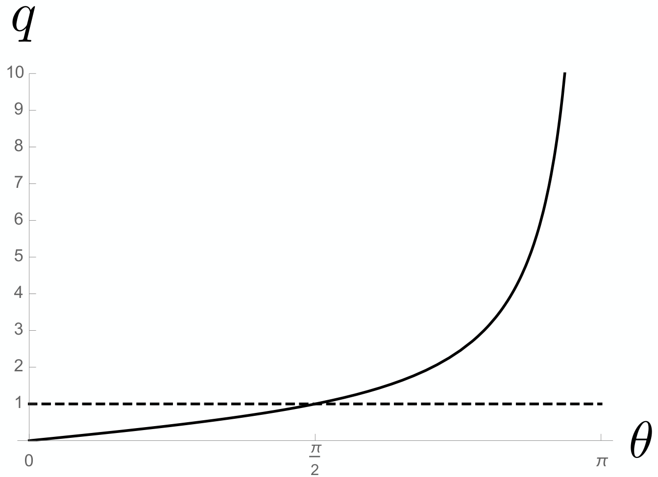
| Fig. 2 | ||||
|---|---|---|---|---|
| (b) | ||||
| (c) | ||||
| (d) |
In sections 5 and 6 we will see that generically the spectral functions of and exhibit Fano resonances, in both the unscreened and screened phases, with various . In our case, the continuum arises from the -dimensional scale invariance associated with the subspace, inherited from the -dimensional scale invariance associated with , and which forces any spectral function to be a power law in , i.e. a continuum. Resonances can then only occur if scale invariance is broken, which we achieve via our marginally relevant Kondo coupling. In our model, the asymmetry is related to particle-hole symmetry breaking, that is, will depend on .
5 Unscreened Phase
In this section we use the results of sections 2 and 3 to determine the excitation spectrum of our system in the unscreened phase, by locating the poles of and in the plane of complex frequency (subsection 5.1), and the corresponding peaks in and for real (subsection 5.2).
Some results for the poles appear already in refs. [31], in the unscreened phase and at small . Indeed, a key result of ref. [31] was that in the unscreened phase, and for any (including ), as a pole moves towards the origin of the complex plane, reaching the origin at precisely . If we then take but remain in the unscreened phase, then the pole moves into the upper half of the complex plane, , signaling the instability towards the screened phase.
Further results appeared in ref. [42], including in particular our central result, the analytic (i.e. non-numerical) result for . In ref. [42], we discussed the movement of poles in as , presented an analytic formula for in terms of and , showed that generically has Fano resonances, derived an analytic form for the pole producing the Fano resonance for just above , and showed that as , producing symmetric Fano resonances (Lorentzians).
In this section we will not only reproduce these results, but also extend them, in particular by exploring in far greater detail the and dependence of the poles in and peaks in . Moreover, we will present analytic results for poles in the limit, which demonstrate conclusively the appearance of Fano resonances in when .
As derived in section 3, we have and , and from eq. (3.73)
| (5.1) |
where from eq. (3.74) we have
| (5.2) |
where denotes the harmonic number.
We can write eqs. (5.1) and (5.2) in terms of field theory quantities using and by replacing with the Kondo temperature , following refs. [31, 32], as follows. In the metric of eq. (2.6), we re-scale to produce dimensionless coordinates,
| (5.3) |
which leaves the metric in eq. (2.6) invariant, except for , so the boundary remains at but the horizon is now at . We also re-scale , which is then dimensionless. After the re-scaling, ’s asymptotic expansion is
| (5.4) |
where represents terms that vanish faster than those shown when , and are completely determined by the terms shown, via the equations of motion. The boundary condition discussed below eq. (3.64) is now , with , and where
| (5.5) |
is our running holographic Kondo coupling, with UV cutoff . If , then if increases, meaning , then exhibits asymptotic freedom, . We thus identify as an anti-ferromagnetic holographic Kondo coupling. If and decreases, so increases, then diverges by definition at the Kondo temperature,
| (5.6) |
Using eq. (5.6) in eq. (5.2) to replace with , we thus find
| (5.7) |
The form of is the same as , but with .
5.1 Unscreened Phase: Poles in the Green’s Function
Clearly in eq. (5.7) has a pole whenever
| (5.8) |
Given values for and , we can thus find the poles of by solving eq. (5.8) for .
Because the form of is the same as , but with , if is a pole of , then will be a pole of . In other words, the poles of and come in pairs mirrored about the imaginary axis in the -plane.
Fig. 4 shows our numerical results for the positions of poles of (black dots) and (gray diamonds) in the complex plane, for the representative value , for five temperatures: . Fig. 4 shows that each of and has a sequence of poles descending down into the complex plane, i.e. with decreasing imaginary part, spaced apart from one another by an amount , and with as .
As decreases, the most significant change in fig. 4 occurs in the position of the “lowest” poles, meaning the poles nearest the origin at (fig. 4 (a). As decreases, the lowest poles move towards the origin (fig. 4 (b)), reach the origin at the critical temperature (fig. 4 (c)), and then move into the upper half of the complex plane (fig. 4 (d) and (e)), signaling an instability. For any other non-zero , the plots of the pole positions are qualitatively similar to those in fig. 4. In particular, as decreases the lowest poles always pass through the origin and into the upper half of the complex plane, signaling an instability.
However, is slightly different. When , so that is real-valued, the only imaginary term in eq. (5.8) is in the argument of the harmonic number, which is . As a result, solutions of eq. (5.8) must have . Clearly, when the particle-hole symmetry is restored. Fig. 5 shows our numerical results for the positions of poles of (black dots) and (gray diamonds) in the complex plane for , for the temperatures , , and . All the poles are now on the imaginary axis, but otherwise we observe similar behavior to the cases: as decreases, the lowest poles in fig. 5 (a) pass through the origin, now at a critical temperature in fig. 5 (b), and then cross into the upper half of the complex plane in fig. 5 (c).
Since the instability always appears as poles passing through the origin and into the upper half of the complex plane, we can determine the critical temperature easily, as the temperature where the poles reach the origin: in eq. (5.8) we set and then solve for , with the result
| (5.9) |
Fig. 6 shows as a function of , which has a maximum at , decreases monotonically as increases, and goes to zero as .
As mentioned in section 1, our results for the movement of differ dramatically from those of the standard (non-holographic) Kondo model, at large and at leading order in perturbation theory in [75]. In that model, the poles are determined by a condition identical to eq. (5.8), but without the term. As a result, the lowest pole sits exactly at for all . The term is thus repsonsible for the non-trivial movement of , relative to the standard Kondo model. Indeed, the term in eq. (5.8) can be viewed as arising from the renormalization of , i.e. as a strong coupling effect arising from working non-perturbatively in both and the ’t Hooft coupling.
We have been able to compute the position and residue of the poles analytically (without numerics) in two limits: and just above (). In each case, we find a residue with non-zero imaginary part, indicating that will exhibit Fano resonances, as we will confirm in subsection 5.2.
In terms of (instead of ), takes a particularly simple form: using eq. (5.9) to re-write eq. (5.7), we find
| (5.10) |
If , or equivalently , then must also be large for to have a pole. The Harmonic numbers grow large either when with , where , or when approaches a negative integer, as apparent from the series representation
| (5.11) |
We are interested in poles near the origin of the complex -plane, rather than poles at large , since the former have a larger effect on the spectral function, so we will only consider the poles where has argument equal to a negative integer. Explicitly, in the in eq. (5.10), near such a pole we use eq. (5.11) to take
| (5.12) |
with . In that approximation, and with , the in eq. (5.10) becomes
| (5.13) |
The pole’s position and residue are then given by
| (5.14) |
where the lowest pole has , and the higher poles have . The residue in eq. (5.14) is purely imaginary, , so (recalling the table in section 4) we expect will have a symmetric Fano resonance.
Eq. (5.10) makes obvious the pole at when . For just above , , we can obtain this pole’s position and residue by expanding eq. (5.10) in around and simultaneously in around . For the expansion in we use
| (5.15) |
where denotes the first derivative of the digamma function . The pole’s position and residue are then given by
| (5.16) |
as derived in ref. [42]. As , both and vanish linearly, i.e. as , with slopes determined by alone. Fig. 7 shows these slopes as functions of . In particular, fig. 7 (b) shows that the magnitude of ’s slope is largest when and decreases monotonically as increases.

The residue in eq. (5.16) is in general complex-valued, so when , the lowest pole in will produce a Fano resonance in . Plugging the in eq. (5.16) into eq. (4.7) gives us the Fano/asymmetry parameter as a function of , shown in fig. 8. Symmetric Fano resonances will occur when , , , where , , and , respectively, corresponding to a Fano anti-resonance, symmetric Fano resonance, and Lorentzian resonance (figs. 2 (b), (c), and (d)), respectively.

5.2 Unscreened Phase: Spectral Function
The spectral function in the unscreened phase is trivial to compute from in eq. (5.10):
| (5.17) |
where we now restrict to real-valued . In our case, vanishes when or , in the latter case vanishing as , ultimately because the Harmonic numbers are asymptotically logarithmic, as mentioned above. Such behavior means our cannot be exactly in eq. (4.3), since involves only powers of , with no logarithms. Nevertheless, we have shown in subsection 5.1 that the lowest pole in generically has residue with non-zero imaginary part, so we expect Fano resonances in at near the real part of the lowest pole’s position, .
Fig. 9 shows as a function of for the representative value and in the regime, namely from (fig. 9 (a)) down to (fig. 9 (b)). From the results in eqs. (5.13) and (5.14), we expect to have a symmetric Fano resonance when equals the real part of the lowest pole’s position, , which is when . Sure enough, for sufficiently high , as in fig. 9 (a), has an approximately symmetric Fano resonance at . As decreases through twelve orders of magnitude, the asymmetry of the resonance appears to increase, although the position changes by only : when , while when . We have confirmed numerically that as decreases through the values in fig. 9, the peak value of the resonance grows as , consistent with the results for and in eq. (5.14). Crucially, the resonance in fig. 9 is not at the particle-hole symmetric value , and so is not the Kondo resonance—as expected, since the Kondo resonance is generically absent at large- in the unscreened phase.

Fig. 10 shows as a function of for from (fig. 10 (a)) down to (fig. 10 (b)), including , corresponding to (fig. 4 (a)), and , corresponding to (fig. 4 (b)). In fig. 10, as decreases, we see four changes in the resonance. First, the peak of the resonance moves towards , following the position of the lowest pole in . For example, compare the position of the peak in at or in fig. 10 (b) (dot-dashed or solid curve, respectively) to the position of the lowest pole in in fig. 4 (a) or (b), respectively. Second, the resonance grows taller, by about an order of magnitude for the values of in fig. 10. Third, the peak grows narrower, also by about an order of magnitude for the values of in fig. 10. Fourth, the Fano/asymmetry parameter increases. For example, for (fig. 10 (a)) and for (fig. 10 (b)).

Fig. 11 shows as a function of for and in the regime, namely for (fig. 11 (a)) down to (fig. 11 (b)). The four trends observed in fig. 10 appear again in fig. 11. First, the resonance moves towards , following the real part of the position of the lowest pole in in the regime, given by in eq. (5.16), which in particular has . Second, the resonance grows taller. Indeed, plugging the results for and of eq. (5.16) into eq. (4.5) reveals that the peak of the resonance increases as . Such power-law growth, rather than logarithmic growth, again indicates that the resonance is not a Kondo resonance. Third, the resonance grows narrower, with a width proportional to the imaginary part of the lowest pole in in the regime, which from eq. (5.16) has . Fourth, the Fano/asymmetry parameter increases. For example, for (fig. 10 (a)) and for (fig. 10 (b)).

In the regime, we expect symmetric Fano resonances when , , , as discussed below eq. (5.16) and in fig. 8. We indeed find such behavior, already at relatively small values of . Fig. 12 shows as a function of for and (a) , (b) , and (c) . We clearly see symmetric Fano (anti-)resonances with (a) , (b) , and (c) , respectively, all consistent with eq. (5.16) and fig. 8.

For the special value nothing breaks the particle-hole symmetry , and all poles of have vanishing real part, as shown for example in fig. 5. When we thus expect a symmetric Fano resonance at for all . Fig. 13 shows as a function of for and from down to (fig. 13 (a)) and from down to (fig. 13 (b)). We indeed find symmetric Fano resonances at for all .

We can also consider in the unscreened phase when , bearing in mind that the unscreened phase is unstable when because has a pole with , as discussed above. Fig. 14 (a) shows , as a function of for and for , namely for and , corresponding to and , respectively (figs. 4 (d) and (e), respectively). We find a mirror version of the four trends observed for in figs. 10 and 11. First, the resonance moves away from , with peak position at . Second, the resonance grows shorter. Third, the resonance grows wider. Fourth, the value of decreases. In particular, for and for . Fig. 14 (b) shows , as a function of for and and . In that case, as expected we find a symmetric Fano resonance at whose height decreases as decreases. All of these behaviors are consistent with the motion of the lowest pole in in the complex plane described in subsection 5.1.

In summary, we have learned two key lessons from the poles in and corresponding resonances in in the unscreened phase. First, we do not see a Kondo resonance, consistent with the expectations of large- Kondo models, where the Kondo effect (screening, phase shift, etc.) occurs only in the screened phase. Second, the resonances we find are all Fano resonances, consistent with our interpretation that -dimensional scale invariance implies a continuum, and our Kondo coupling then breaks scale invariance and produces a resonance that is necessarily immersed the continuum.
6 Screened Phase
In this section we use the results of sections 2 and 3 to determine the excitation spectrum of our system in the screened phase by locating the poles in in the plane of complex (subsection 6.1), and the corresponding peaks in for real (subsection 6.2).
The main results of this section appeared in ref. [42], namely that for just below (), a pole of the form appears in , giving rise to a symmetric Fano resonance in , which is a signature of a Kondo resonance at large . In this section we will present some additional details about these results. Moreover, in appendix D we show, without using numerics, that , but only for , although our methods should easily generalize to any .
As derived in eq. (3.81), in the screened phase
| (6.1) |
and , so we will henceforth discuss only . In the unscreened phase we had the analytic (i.e. non-numerical) result for in eq. (5.2), however, in this section our solutions for will be numerical.
6.1 Screened Phase: Poles in the Green’s Function
Clearly in eq. (6.1) has a pole whenever . (Via eq. (3.81), several other two-point functions have the same poles as well, namely , , , and .) Given values of and , we can thus find the poles in by solving the equation for , which we have done numerically. Our numerical results for the positions of the poles appear in fig. 15, for and with in fig. 15 (a), (b), (c), and (d). When , the poles’ positions agree with those we found in the unscreened phase in subsection 5.1, including in particular the lowest pole, , sitting at the origin of the complex plane. As decreases the most significant change occurs in , which moves straight down the imaginary axis. For any other non-zero , the plots of the pole positions are qualitatively similar to those in fig. 15, except for , where all the higher poles are on the imaginary axis. In particular, for all , including , as decreases the most significant change occurs in , which moves straight down the imaginary axis.
For just below , , we find that is determined by . More specifically, fig. 16 shows that when . In appendix D, for the case we show analytically (i.e. without numerics) that for . Given the mean-field scaling discussed in sec. 2, when , we thus have when .


As mentioned in section 1, a pole in of the form is precisely the manifestation of the Kondo resonance that we expect at large [75]. In other words, in addition to the dynamically generated scale , impurity screening, a phase shift, and so forth, our holographic Kondo model also correctly captures an essential spectral feature of the Kondo effect, namely the Kondo resonance.
6.2 Screened Phase: Spectral Function
Knowing the result of subsection 5.2, that our spectral function generically exhibits a Fano resonance associated with the lowest pole in , and knowing the result of subsection 6.1, that in the screened phase is purely imaginary and simply moves down the imaginary axis as decreases, we can anticipate how will behave in the screened phase. Given that is purely imaginary, and hence does not break particle-hole symmetry , we expect to exhibit a symmetric Fano resonance at . Moreover, given that moves straight down the imaginary axis as decreases, we expect the Fano resonance’s width to increase as decreases.
Our numerical results for in the screened phase confirm these expectations. Fig. 17 shows our numerical results for in the screened phase as a function of real-valued for and , , and . We indeed find only symmetric Fano resonances whose width increases as decreases. We also find that the resonance’s height decreases rapidly as decreases: in fig. 17, decreases by only about , from down to , but the height of the peak drops by roughly two orders of magnitude. As decreases further (not shown in fig. 17), continues to flatten, and indeed, as approaches zero, appears to approach zero for all . All of these features of appear for other values of as well, including .
In the standard (non-holographic) large- Kondo model with Abrikosov pseudo-fermions, the Kondo resonance has width [75]. For , the mean-field behavior then implies the width is . When , reaches a finite value at the minimum of its wine-bottle effective potential. The Kondo resonance then has width , similarly to finite .
Our model also exhibits mean-field behavior, and hence a width when . However, in our screened phase, as decreases our manifestation of the Kondo resonance, i.e. the symmetric Fano resonance in , flattens out, and ultimately disappears, so that at apparently is featureless. What accounts for the difference? In our model, ’s effective potential is apparently unbounded: we found numerically that grows without bound as decreases, because grows without bound. Indeed, as decreases, eventually the solutions for and violate the probe limit: the stress-energy tensor grows without bound, and eventually cannot be neglected in Einstein’s equation. That is unsurprising, given that in our bulk action eq. (2.8), ’s potential is unbounded, being only a mass term, . Presumably, stabilizing ’s potential, for example with a term, would stabilize , and hence stabilize the width of our resonance.
7 Discussion and Outlook
We studied the poles in retarded Green’s functions and the associated peaks in spectral functions in the holographic Kondo model of refs. [31, 32, 33, 34]. We had three main results. First was the holo-ren of our model, which provided the covariant counterterms required to compute the renormalized free energy and one- and two-point functions in our model. Second, at all , we found that generically the poles in our Green’s functions have residue with non-zero imaginary part, giving rise to Fano resonances in spectral functions. Fano resonances occur when a resonance appears in a continuum (in energy) of states. Our continuum comes from -dimensional scale invariance, inherited from -dimensional scale invariance of our holographic CFT. Our resonances are possible because we break scale invariance via our marginally-relevant Kondo coupling. Third, in the screened phase, where , and with just below , we found a pole in of the form , precisely as expected for the Kondo resonance at large [75]. In contrast, in the unscreened phase passed through the origin as decreased through , which was clearly a strong coupling effect: in the standard (non-holographic) Kondo model at large and at leading order in perturbation theory in , in the unscreened phase sits at the origin of the complex plane for all [75].
For the future, some obvious, immediate tasks involve improvements to our model. For example, giving our bulk scalar a quartic self-interaction could not only prevent from diverging at low , and hence maintain the validity of the probe limit at low , but could also prevent our Kondo resonance from disappearing as decreases, as we discussed in subsection 6.2. Indeed, adding a quartic term would introduce an additional dimensionful parameter in our model, which could presumably be fixed by demanding that our Kondo resonance has width when .
However, as discussed in refs. [31, 32], all holographic quantum impurity models to date, including ours, have a fundamentally worrying issue: the spin symmetry group is the gauge group, . Holography provides direct access only to gauge-invariant quantities. As a result, many important quantities that are not spin singlets, such as the magnetization and spin susceptibility, are prohibitively difficult if not impossible to calculate using holography. The obvious route to address this issue is to develop holographic quantum impurity models in which spin is a global symmetry.
We have seen that even a minimal holographic quantum impurity model can produce Fano resonances. Indeed, Fano resonances require simple, common ingredients, and thus are very generic. We therefore expect Fano resonances in practically any holographic quantum impurity model, under the key condition that conformal symmetry is broken at the impurity. (Otherwise, all two-point functions at the impurity are determined by the conformal symmetry, as we mentioned in the section 1.) In fact, more generally we expect asymmetric Fano resonances in practically any holographic system with a UV fixed point, breaking of scale invariance, and breaking of particle-hole symmetry.
Most importantly, we expect our holographic Kondo model, other similar holographic quantum impurity models, and variations of SYK models, to be useful in addressing many of the open questions mentioned in section 1, about EE, quantum quenches, etc. We expect Fano resonances in particular to play a crucial role in developing a precise “dictionary” between theoretical models and experiments.
Acknowledgments
We thank Ian Affleck, Natan Andrei, Piers Coleman, Mario Flory, Antal Jevicki, Henrik Johannesson, Andrew Mitchell, Max Newrzella, and Philip Phillips for helpful conversations and correspondence. A. O’B. is a Royal Society University Research Fellow. J. P. is supported by the Clarendon Fund and St John’s College, Oxford, and by the European Research Council under the European Union’s Seventh Framework Programme (ERC Grant agreement 307955). C.H. is supported by the Ramon y Cajal fellowship RYC-2012-10370, the Asturian grant FC-15-GRUPIN14-108 and the Spanish national grant MINECO-16-FPA2015-63667-P.
Appendices
Appendix A Near-Horizon Expansions in the Screened Phase
In this appendix we determine the near-horizon expansions of the response functions , , , and defined in eq. (3.34) in the screened phase. We use these expansions to fix in-going boundary conditions at the horizon when we solve eq. (3.37) numerically for the response functions.
In this appendix we will switch from the holographic radial coordinate in eq. (2.6) to the coordinate , so that near the horizon, and using eq. (3.2) to translate from to of eq. (3.1),
| (A.1) |
Near the horizon, eqs. (3.17) for the background fields and thus become
| (A.2) |
with regular solutions
| (A.3) |
with integration constants and , which we determine in our numerical solutions by matching with the integration constants in the near-boundary expansions.
Using the above, we can determine the near-horizon expansions of the fluctuations , , and in eq. (3.18). Near the horizon, the constraint eq. (3.18a) becomes
| (A.4) |
with solutions
| (A.5) |
with integration constants and . Inserting eq. (A.5) into eqs. (3.18b) and (3.18c) gives us
| (A.6a) | ||||
| (A.6b) | ||||
to leading order, with the linearly-independent solutions
| (A.7a) | ||||
| (A.7b) | ||||
| (A.7c) | ||||
| (A.7d) | ||||
The most general in-going solution is a linear combination of the solutions with
| (A.8) |
Near the horizon, the definitions of the response functions in eq. (3.33) become
| (A.9a) | ||||
| (A.9b) | ||||
| (A.9c) | ||||
Inserting the two linearly-independent in-going solutions of eq. (A.7) into eq. (A.9) leads to four algebraic equations for the leading near-horizon behavior of the response functions,
| (A.10a) | ||||
| (A.10b) | ||||
| (A.10c) | ||||
| (A.10d) | ||||
with solutions
| (A.11a) | ||||
| (A.11b) | ||||
| (A.11c) | ||||
which are the main results of this appendix. Inserting eq. (A.11) into the general solution for in eq. (3.36) then gives us
| (A.12) |
and hence in-going boundary conditions require that and thus , as advertised in subsection 3.2.2. As a result, the Riccati equations in eq. (3.35) simplify to those in eq. (3.37).
Appendix B Near-Boundary Expansions
In this appendix we determine the general Fefferman-Graham (FG) asymptotic expansions of the fields in our model. As mentioned at the beginning of section 3 these FG expansions involve a number of subtleties, related to the special form of the FG expansion of gauge fields in . In particular, the leading asymptotic mode of the gauge field is the charge instead of the chemical potential , unlike gauge fields in higher-dimensional AdS spacetimes, and moreover the value of affects the FG expansion of the scalar field . As a result, a well-defined space of asymptotic solutions requires keeping fixed, which corresponds to an asymptotic second class constraint on the space of solutions. Such a constraint is unusual, compared to many holographic systems, although the constraint required for Lifshitz asymptotics in Einstein-Proca theory [97, 98] is analogous.
A direct result of the constraint is that, if we allow fluctuations about a background solution to have non-zero variation of , then the background and fluctuations need not have the same FG expansions. Indeed, in that case, higher order fluctuations are increasingly dominant asymptotically, relative to both the background solutions and to the lower order fluctuations. As a result, the small fluctuation approximation breaks down asymptotically, and we are forced to work with a cut-off near the boundary, until fluctuations proportional to are set to zero. In addition, generically no well-defined asymptotic solutions to the full non-linear equations of motion exist, so we must consider the FG expansions of the background and of the fluctuations separately. Below we determine the FG expansions both for the background and the fluctuations, discussing separately fluctuations with and .
Note about Notation:
In this appendix and in appendix C, denotes a quantity that asymptotes to zero like as , with a non-negative integer.
B.1 Expansions of the Background and the Second Class Constraint
Upon choosing a gauge with , the equations of motion for , , and , eqs. (3.12), become
| (B.1a) | ||||
| (B.1b) | ||||
| (B.1c) | ||||
| (B.1d) | ||||
Given the asymptotic form of the metric, as , as long as asymptotically (i.e. the dual operator is relevant), then the gauge field’s leading asymptotic behavior is , with an arbitrary function of time . Moreover, enters ’s equation as a mass term, so that has an “effective mass” , hence affects the FG expansion of . A well-defined space of asymptotic solutions thus requires the (second class) constraint that is fixed. The charge is not automatically conserved by the equations of motion, due to the coupling to the charged scalar field. Charge conservation, therefore, can only be imposed as a boundary condition.
As in ref. [31], we fix such that has dimension , so that our Kondo coupling is classically marginal. The scalar’s effective mass must thus saturate the Breitenlohner-Freedman bound:
| (B.2) |
We want to determine the FG expansions with satisfying the constraint eq. (B.2). Crucially, in the first three equations in (B.1), terms containing time derivatives affect only sub-leading orders in the FG expansion: for the leading non-normalizable and normalizable orders, we can thus ignore all time derivatives in eqs. (B.1). For similar reasons, we can take for the purpose of determining the FG expansions. With these simplifications, eqs. (B.1) become
| (B.3a) | ||||
| (B.3b) | ||||
| (B.3c) | ||||
and hence the FG expansions of the fields are
| (B.4a) | ||||
| (B.4b) | ||||
| (B.4c) | ||||
where , , and are arbitrary functions of time, and represent terms that vanish as faster than those shown, and are completely determined by those shown, via the equations of motion. Inserting eqs. (B.4) into eq. (B.1d), which is the constraint imposed by the gauge invariance, and using eq. (B.2), we find and . The FG expansions are thus parameterized by the arbitrary functions , , and . Moreover, is defined only up to a gauge transformation, . We will refer to eqs. (B.4) as “background FG expansions,” because is required to satisfy eq. (B.2). Fluctuations are allowed to violate eq. (B.2), which leads to different FG expansions, as we will see.
B.2 Expansions of the Response Functions
In the unscreened phase, we want to find the FG expansions of the response functions and , using the Riccati equations in eq. (3.20). As above, to do so we may ignore terms involving time derivatives, i.e. frequency , and we may set , in eq. (3.20), leading to
| (B.5) |
and hence the FG expansions of and are
| (B.6a) | ||||
| (B.6b) | ||||
where and are functions of , and represent terms that vanish as faster than those shown, and are completely determined by those shown, via eq. (3.20).
In the screened phase, we instead need to solve instead the Riccati equations eqs. (3.35), with , as required by in-going boundary conditions at the horizon, as shown in appendix A. Again ignoring terms involving time derivatives, and setting , eqs. (3.35) become
| (B.7a) | ||||
| (B.7b) | ||||
| (B.7c) | ||||
These equations admit two distinct classes of asymptotic solutions, depending on whether or . We present both of these solutions in turn.
For fluctuations with , the defining relations in eqs. (3.33) and the asymptotic solution for in eq. (B.4) imply that asymptotically . Eqs. (B.7) then determine the leading asymptotic behavior of the response functions: , , . In eq. (B.7c), the term is exponentially subleading relative to the other terms, and hence can be ignored. The resulting equation for then admits an exact solution, with asymptotic expansion
| (B.8) |
where is an undetermined function of . Eqs. (B.7a) and (B.7b) then determine
| (B.9a) | ||||
| (B.9b) | ||||
Expanding these then leads to the FG expansions
| (B.10a) | ||||
| (B.10b) | ||||
| (B.10c) | ||||
where , and are undetermined functions of the frequency . If we plug eqs. (B.10) into the defining relations eqs. (3.33), then these asymptotic expansions lead to linear fluctuations that are asymptotically more divergent that the background solutions in eqs. (B.4)—an effect of the asymptotic second class constraint eq. (B.2), which is violated infinitesimally by the linear fluctuations with . The second class constraint also causes the integration constant to enter the asymptotic expansions of and before their corresponding integration constants and . We must therefore determine the asymptotic expansions of and beyond the order where and appear linearly, since these terms enter in the expansions of and .
While fluctuations with have three integration constants, , and , fluctuations with have only one, as we will now show. For fluctuations with , the three response functions have the leading order behavior , , and . Eq. (B.7) then implies that is again given by eq. (B.8), while
| (B.11a) | ||||
| (B.11b) | ||||
Expanding eq. (B.11) using eq. (B.4) then gives the FG expansions
| (B.12a) | ||||
| (B.12b) | ||||
| (B.12c) | ||||
Inserting the expansions for , and for either or into eqs. (3.34), then gives
| (B.13) |
which is of the same form as the unscreened case, eq. (B.6), but now with the constraints
| (B.14) |
where comes from the background solution for the scalar, as discussed below eq. (3.64).
Appendix C Further Details of Holographic Renormalization
In this appendix we summarize some technical results related to the holo-ren in subsection 3.3. In particular, we determine asymptotically the functions , , and , defined in eq. (3.47), up to the relevant order for renormalizing the two-point functions, and we obtain explicit expressions for the renormalized response functions that enter in the two-point functions.
C.1 Determining the Boundary Counterterms
We write and as in eq. (3.49): and . Plugging these into eq. (3.48) and expanding in , and using the fact that , , and are all as , we find
| (C.1) |
where primes denote (see appendix B for the definition of ). A simple power-counting argument using the near-boundary asymptotic expansion of the scalar field in eq. (B.4) suffices to show that in general only terms up to order can potentially contribute to near-boundary divergences, so we can neglect all the right-hand-sides in eqs. (C.1). The resulting equations can then be solved exactly.
The most general solution for can be expressed implicitly in the form
| (C.2) |
where is an integration constant. Expanding this solution for small , we obtain
| (C.3) |
where . The equations for and are linear, with general solutions
| (C.4) |
where is a dummy integration variable, and and are integration constants. Expanding these solutions at small gives us
| (C.5a) | ||||
| (C.5b) | ||||
| (C.5c) | ||||
The integration constants , , correspond respectively to the constants , and in the near-boundary expansions of the response functions in eq. (B.10). This can be deduced as follows. Combining (3.34) and (3.46), and using the expansion in eq. (3.47) and eqs. (C.1), we obtain
| (C.6a) | ||||
| (C.6b) | ||||
| (C.6c) | ||||
where the last equality in eq. (C.6c) follows from the first in eq. (C.1). As in eq. (3.46), the superscript indicates that these response functions are obtained from eq. (3.42), not the full on-shell action. Moreover, taking (see eq. (3.45)) with the in eq. (3.5) gives
| (C.7) |
Eqs. (C.6) and (C.7), together with eqs. (C.1), suffice to show that , and satisfy the corresponding eqs. (B.7), with the important caveat that in eqs. (B.7) is replaced by , i.e. the solution that satisfies the first order eq. (C.7). Since and have the same asymptotic behavior, apart from the values of the coefficients and , , and have near-boundary expansions of the same form as those of , and , and hence they should have the same integration constants. This implies that , and are related to , and , respectively, although the explicit map between these integration constants is rather complicated.
However, the fact that , and satisfy eqs. (B.7) with replaced by , does have implications for the boundary counterterms. We have just argued that the near boundary expansion of is of the same form as that of in eq. (B.10), but with some integration constant that is related to . Since , eq. (C.7) implies that has a near-boundary expansion of the form in (B.4) with
| (C.8) |
If we want to use , and as counterterms to renormalize , and , respectively, we must set and , since these are the values appearing in the near boundary expansions in eq. (B.10). However, eq. (C.8) then forces us to set . This poses no problem for renormalizing , but as we pointed out earlier, an unusual feature of the asymptotic expansions in eq. (B.10) is that and contain divergences that involve , which is a dynamical quantity determined by the near-horizon conditions. Setting will thus not renormalize and . This is similar to cases where a source for an irrelevant operator is turned on perturbatively, much like our , and additional multi-trace counterterms are required [55]. In our case this means and should be considered functions of as well, i.e. and , where should evaluated on the background. These functions can be determined by demanding they satisfy exactly the same equations as and , eq. (B.7).
As discussed in section 3, an additional complication arises due to the logarithmic dependence of the functions , , and on , which forces us to introduce explicit cutoff dependence in the counterterms, to ensure they are local functions of the scalar source. For example, keeping only terms that contribute to the near-boundary divergences we set
| (C.9) |
which suffices to renormalize the on-shell action (evaluated with ), as well as .
We will not give the explicit expressions for the counterterms and here, but they can be constructed as outlined above, and they allow us to obtain the renormalized quantities
| (C.10a) | ||||
| (C.10b) | ||||
| (C.10c) | ||||
where and are determined by the specific choice for the counterterm functions.
C.2 Renormalized Response Functions
To determine the renormalized response functions, and hence the corresponding two-point functions, we need to consider the variation of the one-point functions. Moreover, if we want to allow , then the variations of the one-point functions must be considered at a radial cutoff, and the cutoff should be removed only in the end.
A general variation of the gauge field momentum at a radial cutoff yields
| (C.11) |
where we have used the definitions in eqs. (3.53) and introduced the renormalized response functions
| (C.12) |
Using the fact that for solutions that satisfy ingoing boundary conditions at the horizon, we easily find that the response functions , and are related to those introduced in eqs. (3.30) and (3.33) as , , .
However, since the one-point function associated with the gauge field is given by , we need to express in terms of the variations of the other variables. Namely,
| (C.13) |
where
| (C.14a) | ||||
| (C.14b) | ||||
| (C.14c) | ||||
and we have used that . These renormalized response functions at the radial cutoff are directly related with the physical two-point functions in section 3.
Similarly, the generic variation of the renormalized scalar canonical momenta at the radial cutoff gives
| (C.15a) | ||||
| (C.15b) | ||||
where
| (C.16) | ||||||
These renormalized response functions at the radial cutoff are also directly related with the physical two-point functions in section 3.
Finally using eq. (3.34) and the limits in eq. (C.10), we can remove the radial cutoff to obtain the renormalized response functions
| (C.17a) | ||||
| (C.17b) | ||||
| (C.17c) | ||||
| (C.17d) | ||||
| (C.17e) | ||||
| (C.17f) | ||||
| (C.17g) | ||||
| (C.17h) | ||||
| (C.17i) | ||||
where and are defined in eq. (C.10). Eqs. (C.17) are valid for the screened phase only. In the unscreened phase, the scalar’s response functions and are integration constants determined by imposing boundary conditions on the horizon, while all other response functions vanish.
Appendix D Analytic Derivation of the Lowest Pole in the Screened Phase
In this appendix we present an analytic (i.e. non-numerical) derivation of the behavior of the lowest pole in the screened phase, for .
In this appendix we use the metric in eq. (2.6), but with the re-scaling in eq. (D.1) to produce dimensionless coordinates,
| (D.1) |
which leaves the metric in eq. (2.6) invariant, except for , so the boundary remains at but the horizon is now at . We also re-scale , which is then dimensionless. After the re-scaling, ’s asymptotic expansion is that of eq. (5.4),
| (D.2) |
where here and below represents terms that vanish faster than those shown when , and the boundary condition becomes . We additionally re-scale to produce a dimensionless frequency: . Moreover, in this appendix we exclusively use .
We introduce fluctuations of the defect fields, for example , where is the background solution and is the fluctuation, and similarly , and . In the screened phase, and . In this appendix we will assume the background solution is real, . Next we Fourier transform using , and use the same notation for the Fourier transforms of the fluctuations, for example . Linearizing the equations of motion about in the fluctuations then gives the fluctuation equations (the equivalent of eq. (3.18), but in the coordinates of eq. (D.1)),
| (D.3a) | |||||
| (D.3b) | |||||
| (D.3c) | |||||
| (D.3d) | |||||
where prime denotes , for example .
We want the QNMs, that is, solutions for the fluctuations that are normalizable at the boundary and in-going at the horizon , which exist only for particular [99, 100]. The asymptotic expansions of the fluctuations are
| (D.4) |
To guarantee normalizability, and specifically to guarantee that the asymptotic expansions of the fluctuations do not have terms more divergent than the asymptotic expansions of the background solutions, we must impose , which requires , with the same value of as the background solution .
We parameterize the solutions of eq. (D.3) as
| (D.5) |
where the powers of are determined by the in-going boundary condition at the horizon, is the background solution with , so that asymptotically
| (D.6) |
and now we must solve for , , and , which must be regular at both the boundary and the horizon .
We want the QNM solutions for near , where the condensate is small, or equivalently is negligible. We thus treat as a small correction to the solution in the unscreened phase, that is, we use the background solution with and , where
| (D.7) |
and then determine by solving the equation of motion for the scalar, linearized about the solution with and eq. (D.7), which gives
| (D.8) |
where is a Legendre function of the first kind.
When , we know from subsection 6.1 that the lowest QNM frequency is near the origin of the complex plane, and hence is also small. We thus expand , , and in both and also ,
| (D.9) |
so that now we must solve for the coefficients , , and . For and ,
| (D.10) |
and obeys the same equation as . The only solutions regular at both the boundary and the horizon are , , and . For higher values of and , the equations for the coefficients are inhomogeneous,
| (D.11) |
where obeys the same equation as , but with source . The sources and depend only on solutions at lower order in and . For example, , which implies , which in turn implies . Furthermore, so that . Determining the sources , , and is straightforward but unilluminating, so we will not present explicit results for them. However, the most singular behavior possible at the horizon is , and similarly for and . As a result, solutions regular at the horizon have the form
| (D.12) |
where is a dummy variable, and obeys the same equation as , but with . Regularity of at the boundary requires
| (D.13) |
and a second condition, identical to eq. (D.13), but with and . Regularity of at the boundary requires
| (D.14) |
while regularity of at the boundary requires a condition identical to eq. (D.14), but with , , and . However, using , as mentioned above, and the second regularity condition for , we can show that the regularity condition for is equivalent to that for in eq. (D.14). We are thus left with only eq. (D.14), which will be satisfied only for certain values of . In particular, in our regime of interest, with small and , the solution of eq. (D.14) gives the lowest QNM frequency,
| (D.15) |
Performing the integrals in eq. (D.15) numerically, we find . Given , we have thus shown that for , and in the regime of the screened phase, , as advertised in subsection 6.1.
References
- [1] J. Kondo, “Resistance Minimum in Dilute Magnetic Alloys,” Prog. Theo. Phys. 32 no. 1, (1964) 37–49. http://ptp.ipap.jp/link?PTP/32/37/.
- [2] D. Goldhaber-Gordon, H. Shtrikman, D. Mahalu, D. Abusch-Magder, U. Meirav, and M. A. Kastner, “Kondo Effect in a Single-electron Transistor,” Nature 391 (1998) 156–159.
- [3] S. Cronenwett, T. Oosterkamp, and L. Kouwenhoven, “A Tunable Kondo Effect in Quantum Dots,” Science 281 no. 5376, (1998) 540–544.
- [4] C. Rizzuto, “Formation of Localized Moments in Metals: Experimental Bulk Properties,” Rep. Prog. Phys. 37 no. 2, (1974) 147.
- [5] G. Grüner and A. Zawadowski, “Low Temperature Properties of Kondo Alloys,” in Progress in Low Temperature Physics, D. Brewer, ed., vol. 7, Part B, pp. 591 – 647. Elsevier, 1978.
- [6] K. G. Wilson, “The Renormalization Group: Critical Phenomena and the Kondo Problem,” Rev.Mod.Phys. 47 (1975) 773.
- [7] H. R. Krishna-murthy, J. W. Wilkins, and K. G. Wilson, “Renormalization-group approach to the anderson model of dilute magnetic alloys. i. static properties for the symmetric case,” Phys. Rev. B 21 (Feb, 1980) 1003–1043. http://link.aps.org/doi/10.1103/PhysRevB.21.1003.
- [8] H. R. Krishna-murthy, J. W. Wilkins, and K. G. Wilson, “Renormalization-group approach to the anderson model of dilute magnetic alloys. ii. static properties for the asymmetric case,” Phys. Rev. B 21 (Feb, 1980) 1044–1083. http://link.aps.org/doi/10.1103/PhysRevB.21.1044.
- [9] N. Andrei, “Diagonalization of the Kondo Hamiltonian,” Phys. Rev. Lett. 45 (Aug, 1980) 379–382. http://link.aps.org/doi/10.1103/PhysRevLett.45.379.
- [10] P. Wiegmann, “Exact Solution of s-d Exchange Model at T=0,” Sov. Phys. JETP Lett. 31 (1980) 364.
- [11] N. Andrei, K. Furuya, and J. H. Lowenstein, “Solution of the Kondo problem,” Rev. Mod. Phys. 55 (Apr, 1983) 331–402. http://link.aps.org/doi/10.1103/RevModPhys.55.331.
- [12] A. Tsvelick and P. Wiegmann, “Exact Results in the Theory of Magnetic Alloys,” Advances in Physics 32 no. 4, (1983) 453–713.
- [13] P. Coleman and N. Andrei, “Diagonalisation of the Generalised Anderson Model,” Jour. Phys. C19 (1986) 3211–3233.
- [14] N. Andrei, “Integrble Models in Condensed Matter Physics,” eprint arXiv:cond-mat/9408101 (Aug., 1994) , cond-mat/9408101.
- [15] P. Zinn-Justin and N. Andrei, “The Generalized Multi-channel Kondo Model: Thermodynamics and Fusion Equations,” Nucl. Phys. B528 (1998) 648–682, arXiv:cond-mat/9801158 [cond-mat].
- [16] A. Jerez, N. Andrei, and G. Zaránd, “Solution of the Multichannel Coqblin-Schrieffer Impurity Model and Application to Multilevel Systems,” Phys. Rev. B58 (1998) 3814–3841, arXiv:cond-mat/9803137 [cond-mat].
- [17] P. Coleman, “Mixed Valence as an Almost Broken Symmetry,” Phys. Rev. B35 (Apr, 1987) 5072–5116. http://link.aps.org/doi/10.1103/PhysRevB.35.5072.
- [18] Bickers, N., “Review of Techniques in the Large-N Expansion for Dilute Magnetic Alloys,” Rev. Mod. Phys. 59 (Oct, 1987) 845–939. http://link.aps.org/doi/10.1103/RevModPhys.59.845.
- [19] O. Parcollet and A. Georges, “Transition from Overscreening to Underscreening in the Multichannel Kondo Model: Exact Solution at Large N,” Phys. Rev. Lett. 79 (1997) 4665–4668, arXiv:cond-mat/9707337 [cond-mat].
- [20] O. Parcollet, A. Georges, G. Kotliar, and A. Sengupta, “Overscreened Multi-channel SU(N) Kondo Model: Large-N Solution and Conformal Field Theory,” Phys. Rev. B58 (Aug., 1998) 3794–3813, arXiv:cond-mat/9711192.
- [21] P. Coleman, “Heavy Fermions: Electrons at the Edge of Magnetism,” in Handbook of Magnetism and Advanced Magnetic Materials: Fundamentals and Theory, Kronmuller and Parkin, eds., vol. 1, pp. 95–148. John Wiley and Sons, 2007. [arxiv:cond-mat/0612006].
- [22] P. Coleman, “Heavy Fermions and the Kondo Lattice: a 21st Century Perspective,” ArXiv e-prints (Sept., 2015) , arXiv:1509.05769 [cond-mat.str-el].
- [23] I. Affleck, “A Current Algebra Approach To The Kondo Effect,” Nucl. Phys. B336 (1990) 517.
- [24] I. Affleck and A. Ludwig, “The Kondo Effect, Conformal Field Theory and Fusion Rules,” Nucl.Phys. B352 (1991) 849–862.
- [25] I. Affleck and A. Ludwig, “Critical Theory of Overscreened Kondo Fixed Points,” Nucl.Phys. B360 (1991) 641–696.
- [26] I. Affleck and A. Ludwig, “Universal Non-integer ’Ground State Degeneracy’ in Critical Quantum Systems,” Phys.Rev.Lett. 67 (1991) 161–164.
- [27] I. Affleck and A. Ludwig, “Exact Conformal-field-theory Results on the Multichannel Kondo Effect: Single-fermion Green’s function, Self-energy, and Resistivity,” Phys.Rev. B48 (1993) 7297–7321.
- [28] I. Affleck, “Conformal Field Theory Approach to the Kondo Effect,” Acta Phys. Polon. B26 (1995) 1869–1932, arXiv:cond-mat/9512099.
- [29] A. Hewson, “The Kondo Model to Heavy Fermions,” Cambridge University Press (1993) .
- [30] D. L. Cox and A. Zawadowski, “Exotic Kondo Effects in Metals: Magnetic Ions in a Crystalline Electric Field and Tunnelling Centres,” Advances in Physics 47 no. 5, (1998) 599–942, arxiv:cond-mat/9704103. {}.
- [31] J. Erdmenger, C. Hoyos, A. O’Bannon, and J. Wu, “A Holographic Model of the Kondo Effect,” JHEP 12 (2013) 086, arXiv:1310.3271 [hep-th].
- [32] A. O’Bannon, I. Papadimitriou, and J. Probst, “A Holographic Two-Impurity Kondo Model,” JHEP 01 (2016) 103, arXiv:1510.08123 [hep-th].
- [33] J. Erdmenger, M. Flory, C. Hoyos, M.-N. Newrzella, and J. M. S. Wu, “Entanglement Entropy in a Holographic Kondo Model,” Fortsch. Phys. 64 (2016) 109–130, arXiv:1511.03666 [hep-th].
- [34] J. Erdmenger, M. Flory, C. Hoyos, M.-N. Newrzella, A. O’Bannon, and J. Wu, “Holographic impurities and Kondo effect,” in The String Theory Universe, 21st European String Workshop and 3rd COST MP1210 Meeting Leuven, Belgium, September 7-11, 2015. 2015. arXiv:1511.09362 [hep-th]. https://inspirehep.net/record/1407205/files/arXiv:1511.09362.pdf.
- [35] T. Senthil, S. Sachdev, and M. Vojta, “Fractionalized Fermi Liquids,” Phys. Rev. Lett. 90 no. 21, (May, 2003) 216403, arXiv:cond-mat/0209144.
- [36] T. Senthil, M. Vojta, and S. Sachdev, “Weak Magnetism and Non-Fermi liquids Near Heavy-fermion Critical Points,” Phys. Rev. B69 no. 3, (Jan., 2004) 035111, arxiv:cond-mat/0305193.
- [37] S. A. Hartnoll, C. P. Herzog, and G. T. Horowitz, “Building a Holographic Superconductor,” Phys. Rev. Lett. 101 (2008) 031601, arXiv:0803.3295 [hep-th].
- [38] S. A. Hartnoll, C. P. Herzog, and G. T. Horowitz, “Holographic Superconductors,” JHEP 12 (2008) 015, arXiv:0810.1563 [hep-th].
- [39] P. Nozières and A. Blandin, “Kondo Effect in Real Metals,” J. Phys. France 41 no. 3, (1980) 193–211.
- [40] J. Erdmenger, M. Flory, and M.-N. Newrzella, “Bending branes for DCFT in two dimensions,” JHEP 01 (2015) 058, arXiv:1410.7811 [hep-th].
- [41] D. Friedan and A. Konechny, “On the boundary entropy of one-dimensional quantum systems at low temperature,” Phys. Rev. Lett. 93 (2004) 030402, arXiv:hep-th/0312197 [hep-th].
- [42] J. Erdmenger, C. Hoyos, A. O’Bannon, I. Papadimitriou, J. Probst, and J. M. S. Wu, “Holographic Kondo and Fano Resonances,” arXiv:1611.09368 [hep-th].
- [43] M. Henningson and K. Skenderis, “The Holographic Weyl anomaly,” JHEP 07 (1998) 023, arXiv:hep-th/9806087 [hep-th].
- [44] V. Balasubramanian and P. Kraus, “A stress tensor for anti-de Sitter grvity,” Commun. Math. Phys. 208 (1999) 413–428, arXiv:hep-th/9902121.
- [45] J. de Boer, E. P. Verlinde, and H. L. Verlinde, “On the holographic renormalization group,” JHEP 08 (2000) 003, arXiv:hep-th/9912012 [hep-th].
- [46] S. de Haro, S. N. Solodukhin, and K. Skenderis, “Holographic reconstruction of space-time and renormalization in the AdS / CFT correspondence,” Commun. Math. Phys. 217 (2001) 595–622, arXiv:hep-th/0002230 [hep-th].
- [47] M. Bianchi, D. Z. Freedman, and K. Skenderis, “How to go with an RG flow,” JHEP 08 (2001) 041, arXiv:hep-th/0105276 [hep-th].
- [48] M. Bianchi, D. Z. Freedman, and K. Skenderis, “Holographic renormalization,” Nucl. Phys. B631 (2002) 159–194, arXiv:hep-th/0112119 [hep-th].
- [49] D. Martelli and W. Mueck, “Holographic renormalization and Ward identities with the Hamilton-Jacobi method,” Nucl. Phys. B654 (2003) 248–276, arXiv:hep-th/0205061 [hep-th].
- [50] K. Skenderis, “Lecture notes on holographic renormalization,” Class. Quant. Grav. 19 (2002) 5849–5876, arXiv:hep-th/0209067.
- [51] I. Papadimitriou and K. Skenderis, “AdS / CFT correspondence and geometry,” IRMA Lect. Math. Theor. Phys. 8 (2005) 73–101, arXiv:hep-th/0404176 [hep-th].
- [52] I. Papadimitriou, “Holographic renormalization as a canonical transformation,” JHEP 1011 (2010) 014, arXiv:1007.4592 [hep-th].
- [53] I. Papadimitriou, “Lectures on Holographic Renormalization,” Springer Proc. Phys. 176 (2016) 131–181.
- [54] O. Aharony, S. S. Gubser, J. M. Maldacena, H. Ooguri, and Y. Oz, “Large N field theories, string theory and gravity,” Phys. Rept. 323 (2000) 183–386, arXiv:hep-th/9905111 [hep-th].
- [55] B. C. van Rees, “Holographic renormalization for irrelevant operators and multi-trace counterterms,” JHEP 1108 (2011) 093, arXiv:1102.2239 [hep-th].
- [56] B. C. van Rees, “Irrelevant deformations and the holographic Callan-Symanzik equation,” JHEP 10 (2011) 067, arXiv:1105.5396 [hep-th].
- [57] O. S. An, M. Cvetič, and I. Papadimitriou, “Black hole thermodynamics from a variational principle: Asymptotically conical backgrounds,” JHEP 03 (2016) 086, arXiv:1602.01508 [hep-th].
- [58] T. Faulkner, H. Liu, J. McGreevy, and D. Vegh, “Emergent quantum criticality, Fermi surfaces, and AdS2,” arXiv:0907.2694 [hep-th].
- [59] S. Sachdev, “Bekenstein-Hawking Entropy and Strange Metals,” Phys. Rev. X5 no. 4, (2015) 041025, arXiv:1506.05111 [hep-th].
- [60] S. Sachdev and J.-W. Ye, “Gapless spin fluid ground state in a random, quantum Heisenberg magnet,” Phys. Rev. Lett. 70 (1993) 3339, arXiv:cond-mat/9212030 [cond-mat].
- [61] A. Kitaev, “A simple model of quantum holography,” 2015. http://online.kitp.ucsb.edu/online/entangled15/. Talks for the KITP Strings seminar and Entanglement 2015 program, Feb. 12, Apr. 7, and May 27, 2015.
- [62] J. Polchinski and V. Rosenhaus, “The Spectrum in the Sachdev-Ye-Kitaev Model,” arXiv:1601.06768 [hep-th].
- [63] Y.-Z. You, A. W. W. Ludwig, and C. Xu, “Sachdev-Ye-Kitaev Model and Thermalization on the Boundary of Many-Body Localized Fermionic Symmetry Protected Topological States,” arXiv:1602.06964 [cond-mat.str-el].
- [64] W. Fu and S. Sachdev, “Numerical study of fermion and boson models with infinite-range random interactions,” arXiv:1603.05246 [cond-mat.str-el].
- [65] A. Jevicki, K. Suzuki, and J. Yoon, “Bi-Local Holography in the SYK Model,” JHEP 07 (2016) 007, arXiv:1603.06246 [hep-th].
- [66] J. Maldacena and D. Stanford, “Comments on the Sachdev-Ye-Kitaev model,” arXiv:1604.07818 [hep-th].
- [67] K. Jensen, “Chaos and hydrodynamics near AdS2,” arXiv:1605.06098 [hep-th].
- [68] A. Jevicki and K. Suzuki, “Bi-Local Holography in the SYK Model: Perturbations,” JHEP 11 (2016) 046, arXiv:1608.07567 [hep-th].
- [69] Y. Gu, X.-L. Qi, and D. Stanford, “Local criticality, diffusion and chaos in generalized Sachdev-Ye-Kitaev models,” arXiv:1609.07832 [hep-th].
- [70] D. J. Gross and V. Rosenhaus, “A Generalization of Sachdev-Ye-Kitaev,” arXiv:1610.01569 [hep-th].
- [71] M. Berkooz, P. Narayan, M. Rozali, and J. Sim�n, “Higher Dimensional Generalizations of the SYK Model,” arXiv:1610.02422 [hep-th].
- [72] W. Fu, D. Gaiotto, J. Maldacena, and S. Sachdev, “Supersymmetric SYK models,” arXiv:1610.08917 [hep-th].
- [73] E. Witten, “An SYK-Like Model Without Disorder,” arXiv:1610.09758 [hep-th].
- [74] R. A. Davison, W. Fu, A. Georges, Y. Gu, K. Jensen, and S. Sachdev, “Thermoelectric transport in disordered metals without quasiparticles: the SYK models and holography,” arXiv:1612.00849 [cond-mat.str-el].
- [75] P. Coleman, “Introduction to Many-Body Physics,” Cambridge University Press (2015) .
- [76] A. E. Miroshnichenko, S. Flach, and Y. S. Kivshar, “Fano resonances in nanoscale structures,” Rev. Mod. Phys. 82 (Aug, 2010) 2257–2298.
- [77] T. Faulkner, N. Iqbal, H. Liu, J. McGreevy, and D. Vegh, “Holographic non-Fermi liquid fixed points,” Phil. Trans. Roy. Soc. A 369 (2011) 1640, arXiv:1101.0597 [hep-th].
- [78] J. Göres, D. Goldhaber-Gordon, S. Heemeyer, M. A. Kastner, H. Shtrikman, D. Mahalu, and U. Meirav, “Fano resonances in electronic transport through a single-electron transistor,” Phys. Rev. B 62 (July, 2000) 2188–2194, cond-mat/9912419.
- [79] P. Phillips, “Advanced Solid State Physics,” Cambridge University Press (2012) .
- [80] E. I. Buchbinder, J. Gomis, and F. Passerini, “Holographic Gauge Theories in Background Fields and Surface Operators,” JHEP 12 (2007) 101, arXiv:0710.5170 [hep-th].
- [81] P. Kraus, “Lectures on Black Holes and the AdS(3)/CFT(2) Correspondence,” Lect. Notes Phys. 755 (2008) 193–247, arXiv:hep-th/0609074.
- [82] J. Camino, A. Paredes, and A. Ramallo, “Stable Wrapped Branes,” JHEP 05 (2001) 011, arXiv:hep-th/0104082.
- [83] J. Gomis and F. Passerini, “Holographic Wilson Loops,” JHEP 08 (2006) 074, arXiv:hep-th/0604007.
- [84] S. Kachru, A. Karch, and S. Yaida, “Holographic Lattices, Dimers, and Glasses,” Phys.Rev. D81 (2010) 026007, arXiv:0909.2639 [hep-th].
- [85] S. Harrison, S. Kachru, and G. Torroba, “A Maximally Supersymmetric Kondo Model,” Class.Quant.Grav. 29 (2012) 194005, arXiv:1110.5325 [hep-th].
- [86] L. Susskind and E. Witten, “The Holographic Bound in Anti-de Sitter Space,” arXiv:hep-th/9805114 [hep-th].
- [87] A. Peet and J. Polchinski, “UV / IR Relations in AdS Dynamics,” Phys.Rev. D59 (1999) 065011, arXiv:hep-th/9809022 [hep-th].
- [88] I. Papadimitriou and K. Skenderis, “Correlation functions in holographic RG flows,” JHEP 10 (2004) 075, arXiv:hep-th/0407071 [hep-th].
- [89] I. Papadimitriou and A. Taliotis, “Riccati equations for holographic 2-point functions,” JHEP 04 (2014) 194, arXiv:1312.7876 [hep-th].
- [90] M. Cvetič and I. Papadimitriou, “AdS2 Holographic Dictionary,” arXiv:1608.07018 [hep-th].
- [91] I. Papadimitriou and K. Skenderis, in preparation.
- [92] E. Kiritsis and V. Niarchos, “Large-N limits of 2d CFTs, Quivers and duals,” JHEP 04 (2011) 113, arXiv:1011.5900 [hep-th].
- [93] K. Jensen, “Chiral Anomalies and AdS/CMT in Two Dimensions,” JHEP 1101 (2011) 109, arXiv:1012.4831 [hep-th].
- [94] T. Andrade, J. Jottar, and R. Leigh, “Boundary Conditions and Unitarity: the Maxwell-Chern-Simons System in ,” JHEP 1205 (2012) 071, arXiv:1111.5054 [hep-th].
- [95] H.-C. Chang, M. Fujita, and M. Kaminski, “From Maxwell-Chern-Simons theory in towards hydrodynamics in dimensions,” JHEP 10 (2014) 118, arXiv:1403.5263 [hep-th].
- [96] I. R. Klebanov and E. Witten, “AdS/CFT correspondence and symmetry breaking,” Nucl. Phys. B556 (1999) 89–114, arXiv:hep-th/9905104.
- [97] W. Chemissany and I. Papadimitriou, “Generalized dilatation operator method for non-relativistic holography,” Phys. Lett. B737 (2014) 272–276, arXiv:1405.3965 [hep-th].
- [98] W. Chemissany and I. Papadimitriou, “Lifshitz holography: The whole shebang,” JHEP 1501 (2015) 052, arXiv:1408.0795 [hep-th].
- [99] D. Birmingham, I. Sachs, and S. N. Solodukhin, “Conformal field theory interpretation of black hole quasi- normal modes,” Phys. Rev. Lett. 88 (2002) 151301, arXiv:hep-th/0112055.
- [100] P. K. Kovtun and A. O. Starinets, “Quasinormal Modes and Holography,” Phys. Rev. D72 (2005) 086009, arXiv:hep-th/0506184.