Nonparametric Bayesian label prediction on a graph
Abstract
An implementation of a nonparametric Bayesian approach to solving binary classification problems on graphs is described. A hierarchical Bayesian approach with a randomly scaled Gaussian prior is considered. The prior uses the graph Laplacian to take into account the underlying geometry of the graph. A method based on a theoretically optimal prior and a more flexible variant using partial conjugacy are proposed. Two simulated data examples and two examples using real data are used in order to illustrate the proposed methods.
Keywords:
Binary classification; graph; Bayesian nonparametrics1 Introduction
In this article we consider prediction problems that can be seen as classification problems on graphs. These arise in several applied settings, for instance in the prediction of the biological function of a protein in a protein-protein interaction graph (e.g. Kolaczyk [2009], Nariai et al. [2007], Sharan et al. [2007]), or in graph-based semi-supervised learning (e.g. Belkin et al. [2004], Sindhwani et al. [2007]). We have problems in mind in which the graph is given by the application context and the graph has vertices of different types, coded by vertex labels that can have two possible values, say. The available data are noisy observations of some of the labels. The goal of the statistical procedure is to classify the vertices correctly, including those for which there is no observation available. The idea is that typically, the location of a given vertex in the graph, in combination with (noisy) information about the labels of vertices close to it, should have predictive power for the label of the vertex of interest. Hence, successful prediction of labels should be possible to some degree.
Several approaches for graph-based prediction have been considered in the literature. In this paper we investigate a nonparametric full Bayes procedure that was recently considered in Kirichenko and van Zanten [2017] and that has so far only been studied theoretically. Concretely, we consider a connected, simple graph , with vertices which we denote simply by . We formalize the notion of nonparametric prediction in this setting by postulating the existence of a soft label function
that determines the hard labels that we (partly) observe. The label corresponding to vertex is a Bernoulli random variable with and the ’s are assumed to be independent. The underlying idea is that the “real”, hard labels of the vertices are obtained by thresholding the soft labels at level , i.e. . The are noisy versions of the real hard labels , in the sense that they can be wrong with some positive probability. Specifically, it holds in this setup that . The Bayesian approach proposed in Kirichenko and van Zanten [2017] consists in endowing the soft label function with a prior distribution and determining the corresponding posterior. The priors we consider are described in detail in the next section.
The posterior distribution for that results from a Bayesian analysis can be used for instance for prediction. For the priors we consider, the computation of the posterior mode is closely related to the computation of a kernel-based regression estimate with a kernel based on the Laplacian matrix associated with the graph (e.g. Ando and Zhang [2007], Belkin et al. [2004], Kolaczyk [2009], Smola and Kondor [2003], Zhu and Hastie [2005]). In that sense the method we consider is close to those used in the cited papers. A benefit of the full Bayesian framework is that the spread of the posterior may be used to produce a quantification of the uncertainty in the predictions. Moreover, we specifically consider a full, hierarchical Bayes procedure because of its capability, when properly designed at least, to automatically let the data determine the appropriate value of crucial tuning parameters.
As is well known, the choice of bandwidths, smoothness, or regularization parameters in nonparametric methods is a delicate issue in general. The graph context is no exception in this regard and it is recognized that it would be beneficial to have a better understanding of how to choose the regularization parameters (e.g. Belkin et al. [2006]). The theoretical results in Kirichenko and van Zanten [2017] indicate how the performance of nonparametric Bayesian prediction on graphs depends on both the geometry of the underlying graph and on the “smoothness” of the (unobserved) soft label function . Moreover, for a certain family of Gaussian process priors Kirichenko and van Zanten [2017] gives guidelines for choosing the hyperparameters in such a way that asymptotically optimal performance is obtained.
The aim of the present paper is to provide an implementation of nonparametric Bayesian prediction on graphs using Gaussian priors based on the Laplacian on the graph. Moreover, we investigate numerically the influence of the geometry of the graph and the smoothness of the soft label function, motivated by the asymptotics given in Kirichenko and van Zanten [2017]. In this manner we arrive at recommended choices for tuning parameters and hyper priors that are in line with the theoretical guarantees and that are also computationally convenient.
The rest of this paper is organized as follows. In the next section a more precise description of the problem setting and of the priors we consider are given. Algorithms to sample from the posterior are given in Section 3 and computational aspects are discussed in Section 4. In Section 5 we present numerical experiments. We first apply and test the procedure on two simulated datasets, one involving the path graph and one a small-world graph, respectively. Next we study the performance on real data, considering the problems of predicting the function of a protein in a protein-protein interaction graph, and classifying hand-written digits using a nearest-neighbour graph. Concluding remarks are given in Section 6.
2 Observation model and priors
2.1 Observation model
Again, we start with a connected, simple undirected graph , with vertices denoted by . Associated to every vertex is a noisy hard label . We assume the ’s are independent Bernoulli variables, with
where is an unobserved function on the vertices of the graph, the so-called soft label function. We observe only a subset of all the noisy labels. This can be a random subset of all the , generated in an arbitrary way, but independent of the values of the labels. Note that in this setup we either observe the label of a vertex or not, so multiple observations of the same vertex are not possible.
2.2 Prior on the soft label function
Our prediction method consists in first inferring the soft label function from and subsequently predicting the hard labels by thresholding. We take a Bayesian approach which is nonparametric, in the sense that we do not assume that belongs to some low-dimensional, for instance generalized linear family of functions.
2.2.1 Prior on
To put a prior on we first use the probit link (i.e. the cdf of the standard normal distribution) to write for some function and then put a prior on . To achieve a form of Laplacian regularization, which takes the geometry of the graph into account (e.g. Belkin et al. [2004], Kirichenko and van Zanten [2017], Kolaczyk [2009]) we employ a Gaussian prior with a covariance structure that is based on the Laplacian of the graph . Recall that this is the matrix defined as , where is the diagonal matrix of vertex degrees and is the adjacency matrix of the graph. (See for instance Cvetkovic et al. [2010] for background information.)
We want to consider a Gaussian prior on with a fixed power of the Laplacian matrix as precision (inverse covariance) matrix. As the Laplacian matrix has eigenvalue however, it is not invertible. Therefore we add a small number to all eigenvalues of to overcome this problem. By Theorem 4.2 of Mohar et al. [1991], we know that the smallest positive eigenvalue of satisfies , which motivates this choice. To make the prior flexible enough we add a multiplicative scale parameter as well. Together, this results in a Gaussian prior for with zero mean and precision matrix , where . We then have
To make the connection with kernel-based learning we note that in the corresponding regularized kernel-based regression model, the matrix corresponds to the kernel and the scale parameter to the regularization parameter controlling the trade-off between fitting the observed data and the “smoothness” of the function estimate, as measured by the squared “smoothness” norm .
2.2.2 Prior on
As with all nonparametric methods, the performance of our procedure will depend crucially on the choice of the hyperparameters and , which control the bias-variance trade-off. The “correct” choices of these parameters depends in principle on properties of the unobserved function (or equivalently, the function ). Theoretical considerations in Kirichenko and van Zanten [2017] have shown that good performance can be obtained across a range of regularities of by fixing at an appropriate level, and putting a prior on the hyperparameter , so that we obtain a hierarchical Bayes procedure. The choices for the prior on and for that were shown to work well in Kirichenko and van Zanten [2017] depend on the geometry of the graph . A main goal of the present paper is to investigate numerically whether this dependence is indeed visible when the method is implemented and to investigate choices for and that yield good performance and are computationally convenient as well.
The geometry of the graph enters through the eigenvalues of the Laplacian, which we denote by . (See, e.g., Chapter 7 of Cvetkovic et al. [2010] for the main properties of the spectrum of .) In Kirichenko and van Zanten [2017] the theoretical performance of nonparametric Bayes methods on graphs is studied under the assumption that for some parameter , there exist , and such that for all large enough,
| (1) |
This condition can be verified numerically for a given graph (as is done for instance for certain propotein-protein interaction and small world graphs in Kirichenko and van Zanten [2017]) and can be shown to hold theoretically for instance for graphs that look like regular grids or tori of arbitrary dimensions.
In our notation, the hyper prior for the scaling parameter that was shown to have good theoretical properties in Kirichenko and van Zanten [2017] (under the geometry condition (1)) is the prior with density given by
| (2) |
If the true (unknown) soft label function has regularity , defined in an appropriate, Sobolev-type sense, then this choice for guarantees that the posterior contracts around the truth at the optimal rate, provided the hyper parameter has been chosen such that . Below we investigate the effect of choosing or too high or too low relative to these “optimal” choices.
To understand better how crucial it is to use the prior (2) and to set its hyperparameters just right, we compare it to a slightly simpler choice that is natural here, which is a gamma prior on with density
| (3) |
for certain . This choice is computationally convenient due to the usual normal-inverse gamma partial conjugacy (see e.g. Choudhuri et al. [2007], Liang et al. [2007] in the context of our setting). It introduces two more hyperparameters and . The authors of Choudhuri et al. [2007] and Liang et al. [2007] mention , corresponding to Jeffreys prior, which is improper, but does not result in any computational restrictions. We will see in the numerical experiments that this choice is a reasonable one in our setting as well.
To distinguish between the two priors (2) and (3) in the paper we always call (3) the ordinary gamma prior for , and (2) the generalized gamma prior for .
We remark that since we are considering two competing priors on , we could in principle consider some form of (Bayesian) model selection. We will however see in the numerical experiments that the ordinary gamma prior generally performs better than the generalized gamma. Since the ordinary gamma prior is also preferable from the computational perspective, we would recommend to use the ordinary gamma instead of a combined method.
2.3 Latent variables and missing labels
Combining what we have so far, we obtain a hierarchical model that can be described as follows:
As is well known (cf. Albert and Chib [1993]) an equivalent formulation using an additional layer of latent variables is given by
This is a more convenient representation which we will use in our computations.
We consider the situation in which we do not observe all the labels , but only a certain subset . The labels that we observe, are only observed once. The precise mechanism that determines which ’s we observe and which ones are missing is not important for the algorithm we propose. We only assume that it is independent of the other elements of the model. Specifically, we assume that for some arbitrary distribution on the collection of subsets vertices, a set of vertices is drawn and that we see which vertices were selected and what the corresponding noisy labels are. In other words, the observed data is .
All in all, the full hierarchical scheme we will work with is the following:
| (4) |
Our goal is to compute the posterior and to use it to predict the unobserved labels.
3 Sampling scheme
We use the latent variable approach as in Albert and Chib [1993], Choudhuri et al. [2007], for instance, and implement a Gibbs sampler to sample from the posterior in the setup (4). This involves sampling repeatedly from the conditionals , and . We detail these three steps in the following subsections.
3.1 Sampling from
By construction, we have given that the latent variables , corresponding to the missing observations are independent of those corresponding to the observed labels. We simply have that given and , the variables , , are independent -variables.
As for the latent variables corresponding to the observed labels, we have by (4) that the are independent given and and
where we say that matches if . For , this describes the -distribution, conditioned to be positive. We denote this distribution by . For it corresponds to the -distribution, conditioned to be negative. We denote this distribution by .
Put together, we see that given , and , the are independent and
We note that generating normal random variables conditioned to be positive or negative can for example be done by a simple rejection algorithm or inversion (e.g. Devroye [1986]).
3.2 Sampling from
Since given we know all the ’s, and is independent of all other elements of the model, we have . Next, we have
By plugging in what we know from (4) we get
Completing the square, it follows that
| (5) |
3.3 Sampling from
Again we use that given we know all the ’s, and that is independent of everything else, which gives . Since given , is independent of , we have
| (6) |
Now the method for (approximate) sampling from depends on the choice of the prior for .
3.3.1 Ordinary gamma prior for
If the prior density for is the ordinary gamma density given by (3) we have the usual Gaussian-inverse gamma conjugacy. Indeed, then we have
In other words, in this case we have
3.3.2 Generalized gamma prior for
If the prior density for is the generalized gamma density given by (2) we do not have conjugacy and we replace drawing from the exact conditional , as done in the preceding subsection, by a Metropolis-Hastings step. To this end we choose a proposal density . To generate a new draw for we follow the usual steps:
- 1.
draw a proposal ;
- 2.
draw an independent uniform variable on ;
- 3.
if
where
then accept the proposal as new draw, else retain the old draw .
Note that is indeed proportional to , as required (cf. (6)).
We have considered different proposal distributions in our experiments. Our experiments indicate that a random walk proposal works well.
3.4 Overview of the sampling schemes
For convenience we summarize our sampling scheme, which depends on the prior for that we use.
For the generalised gamma prior (2) we have the following:
For the ordinary gamma prior (3) the algorithm looks as follows:
4 Computational aspects
4.1 Using the eigendecomposition of the Laplacian
In every iteration of either Algorithm 1 or 2 the matrix has to be inverted. Doing this naively can in general be computationally demanding, taking computations, in particular if is not very sparse, i.e. if is a dense graph with many vertices with relatively large degree. To relax the computational burden it can be advantageous to change coordinates and to work relative to a basis of eigenvectors of the graph Laplacian .
To make this concrete, suppose we have the eigendecomposition of the Laplacian matrix , where is the diagonal matrix of eigenvalues of and is an orthogonal matrix of eigenvectors. Computing this decomposition costs us one time computations. We can then parametrise the model by the vector instead of . The corresponding equivalent formulation of (4) is given by
| (7) |
Making the appropriate, straightforward adaptations in the posterior computations, the sampling schemes take the following form in this parametrisation:
For the ordinary gamma prior (3) the algorithm looks as follows:
We note that in this approach we need to invest once in the computation of the spectral decomposition of the Laplacian . This removes the matrix inversions in each iteration of the algorithms. We do remark however that there is a matrix multiplication in line 2 of the algorithms. This is in principle an operation, which is the most expensive operation in each iteration. Moreover, Algorithms 3 and 4 produce samples of , that is, we obtain the posterior samples as vectors of coordinates relative to the eigenbasis of the Laplacian. If we want the samples in the original basis, which is what we need for prediction, we need to multiply all these vectors by .
4.2 A strategy for sparse graphs
Instead of sampling the Gaussian distribution in at once as in (5), it can be advantageous to sample this vector one coordinate at the time.
Denoting by the vector with coordinate removed, standard Gaussian computations show that for every coordinate ,
where
and
This method for sampling from the conditional does not require the eigendecomposition of . In case the power of the Laplacian matrix is an integer, the computations for a fixed only involve the -step neighbors of vertex , which might be computationally attractive in graphs where the number of -step neighbors of each vertex is low. For example, if the number of -step neighbors is bounded by , the complexity of each iteration is .
5 Numerical experiments
5.1 Path graph
To explore some of the issues involved in implementing Bayesian prediction prediction on graphs we first consider the basic example of simulated data on the path graph with vertices. In this case, it is known that the Laplacian eigenvalues are for , with corresponding eigenvectors
This graph satisfies the geometry condition (1) with . To simulate data we construct a function on the graph by setting
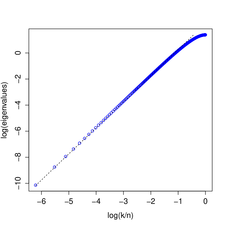
where we choose for . This function has Sobolev-type smoothness , as defined precisely in Kirichenko and van Zanten [2017]. We simulate noisy labels on the graph vertices satisfiying , where is the standard normal cdf. Finally we remove of the labels at random to generate the set of observed labels . The left panel of Figure 1 shows the soft label function and simulated noisy hard labels on the path graph with vertices. In the right panel is plotted against to illustrate that for this graph the geometry condition indeed holds with .

In Figure 2 we visualise the posterior for the soft label function for various graph sizes . Here we used the generalised gamma prior on with , and . These values are suggested by the theory in Kirichenko and van Zanten [2017]. The blue line is the posterior mean and the gray area depicts point-wise credible intervals.


At a first glance it appears that the procedure might be slightly oversmoothing, which could be due to the fact that the posterior for is concentrated at too large values. To get more insight into this issue we compare to posteriors computed with a fixed tuning parameter , set at the “oracle value” which minimises the MSE of the posterior mean, which we determined numerically. The results are given in Figure 3. The posteriors have slightly better coverage than those in Figure 2.



Posterior histograms of the tuning parameter show if we use the generalised gamma prior for , the posterior indeed favours too high values of , compared to the oracle choice. This results in the oversmoothing we observe in Figure 2. See the first two rows of Figure 4.
When instead of the theoretically optimal generalised gamma prior on we use the ordinary gamma prior, we can use the hyper parameters and to ensure that the posterior for assigns more mass close to the oracle tuning parameter. In practice, we do not know the true underlying function, so it is natural to spread the prior mass as much as possible. We can for example choose , corresponding to an improper prior (as in Choudhuri et al. [2007]), or and such that . In Figure 5 we plot the ordinary gamma prior density corresponding to (blue dashed line) and the generalised gamma prior densities for various (black lines). Since the ordinary gamma assigns more mass to smaller values of , we might hope that if we use that prior on , we get a posterior closer to the oracle and hence reduce the oversmoothing problem.


Figure 6 visualises the posteriors that we get for the soft label function when using the ordinary gamma prior with . We see that indeed we get better posterior coverage than in Figure 2. The third row in Figure 4 confirms that when using the ordinary gamma prior on , the posterior for puts more mass around the optimal value.
5.1.1 Impact of prior smoothness
In the paper Kirichenko and van Zanten [2017] it was suggested to take the power of the Laplacian equal to , where is the number appearing in the geometry condition (1) and is a tuning parameter that quantifies the smoothness of the prior in some sense. It was proved that when combining this with the generalised gamma prior (2) on , we get good convergence rates if the Sobolev-type smoothness of the true soft-label function is less than . This might suggest that it is advantageous to set high, since then the theory says that we get good rates across a large range of regularities of the true function. On the other hand, setting higher means we favour smooth functions more. This could potentially lead to oversmoothing and hence to poor posterior coverage. In this section we investigate this issue numerically.
In Figure 7 we use the generalised gamma prior on . We plot the posterior for , varying from left to right and from top to bottom. In the top row . Since this is less than , the theory suggests that we are undersmoothing too much and will get sub-optimal convergence rates. The figure seems to confirms this. In the middle row we have . This means the prior smoothness matches the true smoothness, which is asymptotically a good choice according to the theory. This is the same picture as in Figure 2. In the bottom row . In this case the prior smoothness is larger than the true smoothness . However, the theory says that we should still get a good convergence rates, because to compensate for the smoothness mismatch the posterior for will automatically charge smaller values of more. In the simulations we see that the result is indeed not dramatic, but that the procedure is in actual fact oversmoothing somewhat, resulting in worse posterior coverage.
Figure 8 gives the same plots when using the ordinary gamma prior on , with . We see essentially the same effects, but the effect of choosing too small is a bit more pronounced. In terms of posterior coverage the ordinary gamma prior does a bit better, although it gives too conservative credible sets when is set too low.


5.2 Small-world graph
In this section we consider simulated data on a small-world graph obtained as a realization of the Watts-Strogatz model (Watts and Strogatz [1998]). The graph is obtained by first considering a ring graph of nodes. Then we loop through the nodes and uniformly rewire each edge with probability . We keep the largest connected component and delete multiple edges and loops resulting in the graph in Figure 9 with nodes.


We numerically determine the eigenvalues and eigenfunctions of the graph Laplacian and define a function on the graph by
where we choose for to have Sobolev-type smoothness (cf. Kirichenko and van Zanten [2017]). As before we assign labels to the graph according to probabilities , where is the distribution function of the standard normal distribution. We remove the label of of the nodes. The aim is to predict these using the observed labels.
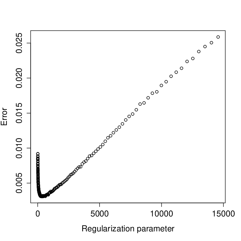
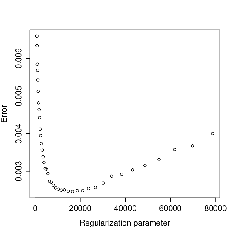
In this case it is hard to visualise smooth functions on the graph and hence to visualise the entire posterior distribution of the soft label function. Instead we analyse the quality of the procedure by plotting credible intervals for the soft label function at randomly selected vertices of which we have not observed the noisy labels. Figure 10 gives these plots for the procedure with the generalised gamma prior on (left), the ordinary gamma prior on with (middle), and the fixed oracle choice of (right). At the bottom left and middle the posteriors for are shown. The bottom right is a plot of the MSE of the posterior mean corresponding to a fixed as a function of that . The point where it is minimal is the oracle choice of .


Also in this example we observe that with the theoretically optimal generalised gamma prior on we are shrinking a bit too much, resulting in particular in credible intervals not containing the true soft label. When using the ordinary gamma prior the performance is closer to the oracle procedure. The bottom row of Figure 10 confirms that with the ordinary gamma prior the posterior for is closer to the oracle choice.
5.2.1 Impact of hyper parameters
We have determined numerically that the graph under consideration satisfies the geometry condition (1) with , see the right panel of Figure 9. The results of Kirichenko and van Zanten [2017] thus suggest to use as prior on the Laplacian to the power for parameter that determines the prior smoothness. Also for this example we have investigated the impact of different choices.
In Figure 11 illustrate what happens if is chosen too low. On the left we see that the procedure with the generalised gamma prior on oversmooths quite dramatically. The bottom row of the figure shows that the posterior for puts too little mass around the oracle in that case. The plots in the middle corresponds to ordinary gamma prior on with . This performs much better, close to procedure with oracle choice of shown on the right. In Figure 12 the parameter is chosen too high. Here all three procedures have comparable performance. All oversmoothing a bit too much due to the fact that the power of the Laplacian becomes too large. This is in line with what we saw for the path graph.


If we choose the parameter correctly, i.e. is this case, and only choose different values for the hyper parameter we only change the prior smoothness of , without changing the prior on . Figures 13 and 14 illustrate the effect. In the first we set , which is too low relative to the smoothness of the true soft label function, in the second one , which is too high. We clearly see the effect on the width of the credible intervals. The effect on coverage is not very large.


5.2.2 Impact of missing observations
To assess the impact of the percentage of missing observations we increase the level from to , and . We observe in Figures 15, 16 and 17 that as the percentage of missing observations increases, the posterior of is more spread out and there is more uncertainty in the function estimates, as is to be expected. In the most extreme case of missing labels we observe that the generalised gamma prior on results in quite severe oversmoothing. In the histogram we see that the posterior for puts too little mass around the oracle choice of in that case. The inverse gamma prior has a much better performance, and remains comparable to the oracle choice.


5.3 Function prediction in a protein-protein interaction graph
To test the nonparametric Bayes procedure on real data we adapt the case study from Kolaczyk [2009], Section 8.5. The example is about the prediction of protein function from a network of interactions among proteins that are responsible for cell communication in yeast. For more information about the background of the experiment set-up, see Kolaczyk [2009].
The protein interaction graph is shown on the left in Figure 18. A vertex in the graph is labelled according to whether or not the corresponding protein is involved in so-called intracellular signaling cascades (ICSC), which is a specific form of communication. We have randomly removed of the labels and we apply our Bayesian prediction procedure to try and recover them from the observed labels.


In view of the findings in the preceding sections we apply the procedure with the ordinary gamma prior on with . Numerical computation of the Laplacian eigenvalues shows that in this case the geometry condition is fulfilled with , see the right panel of Figure 18. We use this value in the procedure. The parameter that determines the prior smoothness of is set to . This is a conservative choice, in order to avoid oversmoothing. We now run our algorithm to produce credible intervals for the soft label function at the vertices of which we did not observe the labels.

Figure 19 shows the results, together with the true labels that we removed. We see that if we predict the missing labels by thresholding the posterior means at , we have a misclassification rate of . If we repeat the procedure times, every time removing different labels at random, we obtain an average misclassification rate of . To assess this, we also computed -nearest neighbour (-NN) predictions for various . We found average missclassification rates of for one -NN, for -NN and for -NN. Hence in terms of prediction performance our procedure is comparable to -NN with the oracle choice of . This illustrates that in line with the theory, our procedure succeeds in automatically tuning the appropriate degree of smoothing. Moreover, the Bayes procedure has the advantage that in addition to predictions, we obtain credible intervals as an indication of the uncertainty in the predictions.
5.4 MNIST digit prediction
So far we have considered examples with graphs that satisfy the geometry condition (1). For such graph we have theoretical results that provide some guidelines for the construction of the prior and choices of the hyper parameters. In principle however, we can also apply our procedure to graphs that do not satisfy (1) for some . It is intuitively clear that a condition like (1) should not always be necessary for good performance. If we use the ordinary gamma prior on and set at a conservative (not too high) value, we can just apply our procedure and should still get reasonable results if the graph geometry and the distribution of the labels are sufficiently related. In this section we briefly investigate such as case.
The MNIST dataset of handwritten digits has a training set of thousand examples and a test set of thousand. The digits are size-normalized and centered in a fixed-size image. The dataset is publicly available at http://yann.lecun.com/exbd/mnist. We have randomly selected a subsample of consisting of only the digits and of which in are the training set and are from the test set. Our goal is to classify the images from the test set. To turn this into a label prediction problem on a graph we construct a graph with nodes, corresponding to the images. For each image we determined the closest images in terms of pixel-distance and connected the corresponding nodes in the graph by an edge. The resulting graph is shown in Figure 20. The eigenvalue plot suggests that the graph does not satisfy the geometry condition to the extent that the preceding graphs did.


The picture indicates that predicting the missing labels in this graph is not a very hard problem. And indeed, our procedure performs well in this case. We classify all missing labels correctly, with very high certainties. See Figure 21.


6 Concluding remarks
We have described a nonparametric Bayes procedure to perform binary classification on graphs. We have considered a hierarchical Bayesian approach with a randomly scaled Gaussian prior as in the theoretical framework in Kirichenko and van Zanten [2017]. We have implemented the procedure with the theoretically optimal prior from Kirichenko and van Zanten [2017] and a variant with a different prior on the scale, which exploits partial conjugacy and has some more flexibility.
Our numerical experiments suggest that good results are obtained when using Algorithm 2, i.e. using the ordinary gamma prior on the scale. Suggested choices for the hyper parameters are and . Here is the geometry parameter appearing in the geometry condition (1) and can be determined numerically from the spectrum of the graph Laplacian. The parameter reflects prior smoothness and should not be set too high (e.g. or ), to avoid oversmoothing.
In view of computational complexity it might be more advantageous to consider other methods to adaptively find the tuning parameter, such as empirical Bayes methods. Also, it might be sensible to modify the prior by truncating the -dimensional Gaussian prior on to a lower dimensional one by writing a series expansion for and truncating the sum at a random point, similar to the approach in Liang et al. [2007] for instance. It is conceivable that in this way the procedure becomes both more flexible in terms of adaptation to smoothness and will also computationally scale better to large sample size . We intend to investigate this in future work.
References
- Albert and Chib [1993] Albert, J.H., Chib, S., 1993. Bayesian analysis of binary and polychotomous response data. Journal of the American statistical Association 88, 669–679.
- Ando and Zhang [2007] Ando, R.K., Zhang, T., 2007. Learning on graph with laplacian regularization. Advances in neural information processing systems 19, 25.
- Belkin et al. [2004] Belkin, M., Matveeva, I., Niyogi, P., 2004. Regularization and semi-supervised learning on large graphs, in: International Conference on Computational Learning Theory, Springer. pp. 624–638.
- Belkin et al. [2006] Belkin, M., Niyogi, P., Sindhwani, V., 2006. Manifold regularization: A geometric framework for learning from labeled and unlabeled examples. Journal of machine learning research 7, 2399–2434.
- Choudhuri et al. [2007] Choudhuri, N., Ghosal, S., Roy, A., 2007. Nonparametric binary regression using a gaussian process prior. Statistical Methodology 4, 227–243.
- Cvetkovic et al. [2010] Cvetkovic, D.M., Rowlinson, P., Simic, S., 2010. An introduction to the theory of graph spectra. Cambridge University Press New York.
- Devroye [1986] Devroye, L., 1986. Non-uniform random variate generation. Springer-Verlag New York.
- Kirichenko and van Zanten [2017] Kirichenko, A., van Zanten, H., 2017. Estimating a smooth function on a large graph by bayesian laplacian regularisation. Electronic Journal of Statistics 11, 891–915.
- Kolaczyk [2009] Kolaczyk, E.D., 2009. Statistical analysis of network data. Springer.
- Liang et al. [2007] Liang, F., Mao, K., Liao, M., Mukherjee, S., West, M., 2007. Nonparametric bayesian kernel models. Department of Statistical Science, Duke University, Discussion Paper , 07–10.
- Mohar et al. [1991] Mohar, B., Alavi, Y., Chartrand, G., Oellermann, O., 1991. The laplacian spectrum of graphs. Graph theory, combinatorics, and applications 2, 12.
- Nariai et al. [2007] Nariai, N., Kolaczyk, E.D., Kasif, S., 2007. Probabilistic protein function prediction from heterogeneous genome-wide data. PLoS One 2, e337.
- Sharan et al. [2007] Sharan, R., Ulitsky, I., Shamir, R., 2007. Network-based prediction of protein function. Molecular systems biology 3, 88.
- Sindhwani et al. [2007] Sindhwani, V., Chu, W., Keerthi, S.S., 2007. Semi-supervised gaussian process classifiers., in: IJCAI, pp. 1059–1064.
- Smola and Kondor [2003] Smola, A.J., Kondor, R., 2003. Kernels and regularization on graphs, in: Learning theory and kernel machines. Springer, pp. 144–158.
- Watts and Strogatz [1998] Watts, D.J., Strogatz, S.H., 1998. Collective dynamics of ‘small-world’networks. nature 393, 440–442.
- Zhu and Hastie [2005] Zhu, J., Hastie, T., 2005. Kernel logistic regression and the import vector machine. Journal of Computational and Graphical Statistics 14, 185–205.