Light-hole Exciton in Nanowire Quantum Dot
Abstract
Quantum dots inserted inside semiconductor nanowires are extremely promising candidates as building blocks for solid-state based quantum computation and communication. They provide very high crystalline and optical properties and offer a convenient geometry for electrical contacting. Having a complete determination and full control of their emission properties is one of the key goals of nanoscience researchers. Here we use strain as a tool to create in a single magnetic nanowire quantum dot a light-hole exciton, an optically active quasiparticle formed from a single electron bound to a single light hole. In this frame, we provide a general description of the mixing within the hole quadruplet induced by strain or confinement. A multi-instrumental combination of cathodoluminescence, polarisation-resolved Fourier imaging and magneto-optical spectroscopy, allow us to fully characterize the hole ground state, including its valence band mixing with heavy hole states.
pacs
78.67.Uh,78.55.Et,42.30.KqI Introduction
Semiconductor quantum dots are seen as important elements for integrated quantum simulation and communication.[1, 2, 3] They can act as static qubits, encoding information either onto their orbital or spin state. They can also serve as a deterministic source of flying qubits using single[4, 5] or entangled photons.[6, 7, 8] In this perspective, hole spins are particularly interesting because of their weak hyperfine coupling to surrounding spin bath compared to electrons.[9, 10] Furthermore working with light-holes pave the way to new information technology protocols like direct manipulation of the hole spin state with RF fields,[11] efficient control of a magnetic impurity spin coupled to a quantum dot,[12] or spin state tomography of the electron inside the dot.[13] However most of the previous studies have concerned so far heavy-hole states, because they are energetically favored for a majority of quantum dot heterostructures for which confinement and strain lift the degeneracy of the valence band.[14, 15] Hence a way to address light-holes is to promote them as the valence band ground state by engineering the strain inside the dot. For epitaxially grown dots this requires technologically intensive methods, such as the fabrication of deformable membranes containing the dots.[16] Another very promising strategy is to embed the dot inside a nanowire.[17] This bottom-up approach produces high quality heterostructures. It offers a way to control both the carriers confinement through the geometrical shape of the dot, and its internal strain by adding a shell of a different material around the nanowire core.[18, 19] To be short, in most nanostructures the low-gap material has a larger lattice parameter. In a flat quantum dot as resulting from Stranski-Krastanow growth, it is well known that the hole ground state has a main heavy-hole character. The most frequent case is that of InAs dots in GaAs, but this is true also for CdTe dots in ZnTe.[20] This is due to the stronger effect of confinement along the growth axis, and to the strongest component of the mismatch strain which is compressive in the plane. In a core-shell nanowire made of the same materials, the confinement is stronger in the plane, and the strongest component of the mismatch strain is compressive along the axis. As a result, both confinement and mismatch strain conspire to make the ground state a light-hole state.[19] When increasing the height of a quantum dot in a nanowire, a crossing is expected, from the heavy-hole ground state in a flat quantum dot to a light-hole ground state in an elongated quantum dot.[18] Note that nanowire structures are very flexible, and a heavy-hole ground state can be found also in a core-shell nanowire if the lattice mismatch induces a tensile strain in the core.[19] An additional important property of a semiconductor nanowire is that it acts as a dielectric antenna, modulating the coupling of the different exciton transitions to light modes which changes their radiation pattern. [21, 5, 22, 23, 24]
Here we provide a complete study of a light-hole quantum dot (QD) in a core-shell nanowire. The dot contains a large fraction of magnetic dopants in order to enhance the Zeeman shift for spintronics applications. This prevents a direct spectroscopic evidence of its light-hole character by measuring its fine structure.[16] We show nevertheless that the detailed observation of the polarisation state of the QD far field radiation pattern is enough to prove its light-hole nature and provides a wealth of information about its mixing with heavy-hole states. Our results are in agreement with numerical simulations of the QD emission within the full nanowire structure. It is confirmed by studying the giant Zeeman shift and the polarisation of the excitonic transition under an external magnetic field. The magneto-optical spectroscopy reveals a heavy-hole excited state at high field, thus providing an order of magnitude for the valence band splitting. Our method is simple, and requires no extra processing of the sample[25, 16] as far as the nanowire is isolated from its neighbours.
II Light-hole and heavy-hole properties and anisotropy

The distinction between light- and heavy-hole arises when the top of the valence band fourfold degeneracy of zinc-blende semiconductors is lifted by, for instance, strain or confinement. Generally, a relevant axis of symmetry appears, such as the growth axis for self-assembled quantum dots or a nanowire. Eigenstates are then Kramers doublets, characterized by the projection of their total spin onto for the electron (), the light-hole (LH, ) and the heavy-hole (HH, ). The HH has a strong magnetic anisotropy, with its spin along but a vanishing Landé factor in the normal -plane. It exhibits also a strong optical anisotropy, with dipolar electric transitions matrix elements towards electron states in the -plane (called transitions hereafter), see Fig. 1(a). By contrast, the LH has a finite Landé factor in the -plane and a smaller one along . Optically, it presents both and polarised transition matrix elements.
We use the hole formalism to describe the top of the valence band: this is more convenient if one has in mind the optical manipulation of holes in a quantum dot [16] or carrier induced magnetic interactions in a dilute magnetic semiconductor.[26] As a result, the hole ground state is at lower energy, and the light-hole/heavy-hole splitting is negative if the ground state is a light hole. implies a LH ground state. However, in real life quantum dot, confinement potential and strain (uniform and inhomogeneous) create additional anisotropy components which break the circular symmetry around and hence mix the light- and heavy-hole states. This mixing is usually described by two additional complex numbers and .[27] In appendix B, we show in details that the resulting Hamiltonian, with one real number and two complex numbers and , is the most general spin Hamiltonian describing an isolated spin quadruplet and respecting time reversal symmetry. All three terms have various origins, including uniform and inhomogeneous strain, and confinement. As a consequence of the mixing the true QD hole eigenstates are linear combinations of the pure heavy- and light-hole states defined by , and the resulting dipole transitions and spin properties are changed accordingly.
The spin Hamiltonian takes a much simpler form in the frame which diagonalizes the anisotropy tensor (see appendix B). It then depends only on two real parameters: which describes the LH/HH splitting along the principal anisotropy axis and which describes the transverse anisotropy in the plane. Three Euler angles , and are necessary to characterize the transformation from the laboratory frame to the anisotropy frame. If , and are the spherical coordinates of axis . characterizes the direction of transverse anisotropy. The parameter measured in the laboratory axes does not really represent a mixing, but the result of the tilt between and . We stress this physical interpretation of the two "mixing parameters" measured in the laboratory frame, because it has direct practical consequences: describes a real mixing, which requires that a shear strain be applied in order to compensate for it.[16] On the other hand the effect of (which can also be due to strain and confinement anisotropy) can be compensated by an appropriate tilt of the optical axis.
In our setup we collect the nanowire light by placing a microscope objective (numerical aperture NA=0.72) on the axis [Fig. 1(b)]. A set of additional optical elements allows to image onto a CCD camera the intensity emitted in a direction .[23, 24] Figures 1(c-d) represent the theoretical colormaps of for a and transition respectively, assuming that the QD is surrounded by an infinite medium made of ZnTe for illustration purpose first. The radial coordinate is equal to and the polar angle is equal to . The two radiation patterns differ dramatically, and could be enough to discriminate light- and heavy-hole emission. Nevertheless, they are significantly affected by the nanowire geometry and by the imperfection of the collection objective. Note that while the dipole emission does not radiate along the optical axis, it does generate light towards larger angles within our experimental numerical aperture, which is collected by our objective [see Fig. 1(d)]. A more precise description of the radiated field comes from the polarisation of the light emitted in a given direction. It is projected by the objective onto a state of polarisation in the plane, represented in Fig. 1(c-d) by the green curves which follow the electric field vector over one optical period. It results in an ellipse whose aspect ratio changes from a perfect circle for a pure to a single line for a pure linear polarisation state. Here again, striking differences exist between and transitions. One important message of our work is that this polarisation analysis for a large set of emission directions provides unambiguous, quantitative informations about the hole character and the valence band mixing.
III Experimental setup and results
III.1 Sample fabrication

Our system is a single (Cd,Mn)Te QD inserted along a <111> ZnTe/(Zn,Mg)Te core/shell nanowire grown by molecular beam epitaxy (see Supplemental Material [28]). [29, 30] The dot is largely doped with Mn atoms (Mn concentration 10%), making it a dilute magnetic semiconductor structure. Due to the nature of the growth, the axial core growth after the quantum dot insertion leads to the formation of a ZnTe shell. A final (Zn,Mg)Te shell is further grown on the resulting tapered-shape nanowire. The wire is standing perpendicular to the substrate in a region of low nanowire density, allowing its study by micro-photoluminescence (µPL) without exciting its neighbours. The PL spectrum at 5K [Fig. 2(a)] exhibits an emission peak centered at , which is related to the exciton recombination in the ZnTe core,[29, 19, 31] and a second one at , which is attributed to the quantum dot luminescence. The presence of the Mn atoms significantly broadens the emission from the QD because of the magnetization fluctuations randomly shifting the exciton line in time through the giant Zeeman effect. The nanowire is also studied by low-temperature cathodoluminescence (CL). The electron beam is along axis . The standard SEM image [Fig. 2(b)] gives access to the geometrical parameters of the wire. The CL signal [Fig. 2(c-d)] provides information about the regions from where light is emitted. Most of the ZnTe luminescence comes from a large region at the base of the nanowire, while the signal attributed to the quantum dot is well localized at a height of from the nanowire base. We note that the spatial width of this signal is related to the diffusion of free electron and holes in the nanowire before they recombine in the dot. It does not correspond to the QD size (, measured independently by energy-dispersive x-ray spectroscopy.[32] CL spectroscopy on similar structures confirms that the well-isolated emission line at , which is also well spatially confined, is related to a single longitudinal QD, while eventual radial (Cd,Mn)Te structures would emit at a higher energy, above .[33] Finally, antibunching experiment on similar emitters without magnetic doping revealed a single photon emission with , confirming the 3D confinement of the carriers inside the dot.[34] Such experiment could not be performed on our magnetically-doped dots yet because of the line broadening resulting from the large magnetic doping of the dot.
III.2 Fourier microscopy results
Let us first compare the unpolarised far field radiation pattern of the ZnTe emission [Fig. 3(a)] to the one of the QD [Fig. 3(c)]. Both present a single lobe of emission whose center is slightly displaced from the origin. We attribute this off-centering to a geometrical tilt of the NW axis with respect to , different from the previous QD tilt previously introduced in the spin Hamiltonian. However, we note on the cross-sections that the angular divergence of the ZnTe emission is definitely smaller than the QD one, which features a dip at its center. This is a first hint for a LH emission from the QD as the transition reinforces light emission at large angles [Fig. 1(d)]. Independent measurements of the objective collection efficiency show that the latter drops dramatically for (see Supplemental Material ([28]). This does not affect the comparison between the two lines, but prevent us to attempt a direct comparison with the calculated patterns of Fig. 1(c-d). Another issue is that the ZnTe emission takes place in a region where the nanowire diameter is such that it strongly guides light along the axis. Even more, due to the nanowire cone shape, the guided mode waist increases adiabatically, and hence its angular divergence decreases - a mechanism which is exploited in photonic wires to maximize light collection from single QD.[5, 24] On the contrary, at the QD location the nanowire diameter is too small to allow an efficient guiding effect.

The difference between ZnTe and QD emission is dramatically highlighted when comparing their linearly polarised radiation patterns. In the case of ZnTe emission they remains similar to the unpolarised one, whatever the polariser direction. On the contrary, the QD emission patterns break the revolution symmetry around . We observe two lobes, off-centered and symmetrically placed on both sides of the optical axis along the direction of polarisation. The lobe intensity decreases at large angle because of the loss of collection efficiency otherwise it would be maximum at the edge of the image as in Fig. 1(b). We also note that there is a 20% intensity imbalance between the two lobes. A convenient way to reinforce the information about the polarisation state of the far field, without the influence of its intensity, is to plot the Stokes parameters [35] and , where is the far field intensity for a linear polariser set at angle . The degree of linear polarisation (DLP) is equal to . In the case of the ZnTe line, both Stokes parameters are homogeneous and very close to 0, with a DLP averaged over all measured directions of light 2%. On the contrary, the QD Stokes parameters are varying with from very large positive values to very negative ones, displaying a characteristic 4-quadrant symmetry. S2 is similar to S1 rotated by . The average DLP is 40%. This is a direct consequence of the polarisation properties sketched in green in Fig. 1(c-d).
Experimental results were compared to far field patterns derived from simulations of the electromagnetic field in the whole nanowire structure by a finite element software and taking into account all the experimental imperfections of our imaging setup (see Supplemental Material [28]). The emitter is modeled by an oscillating dipole . The dipole matrix elements are determined by diagonalizing the hole Hamiltonian including valence band mixing, and considering all possible transitions between the ground hole state and the electron states. For the ZnTe core [Fig. 3(b)], we sum the intensities coming from dipoles emitting at different positions along the nanowire axis, with weights corresponding to the CL intensity in Fig. 2(d). For the QD [Fig. 3(d)], the dipole is fixed at the QD position. The agreement with experimental data is very good. Looking at the unpolarised QD pattern, the effects of the valence band mixing rates and are entangled. However, the unbalanced intensity lobes (central pannel) reflect with its phase, while the linear polarisation observed on S1 close to the optical axis reflects and its phase. The mixing rates are small, hence the QD hole state is essentially (97%) LH. Yet non zero valence band mixing is necessary to properly explain the fine features found in the experimental data.
III.3 Magneto-optical spectroscopy
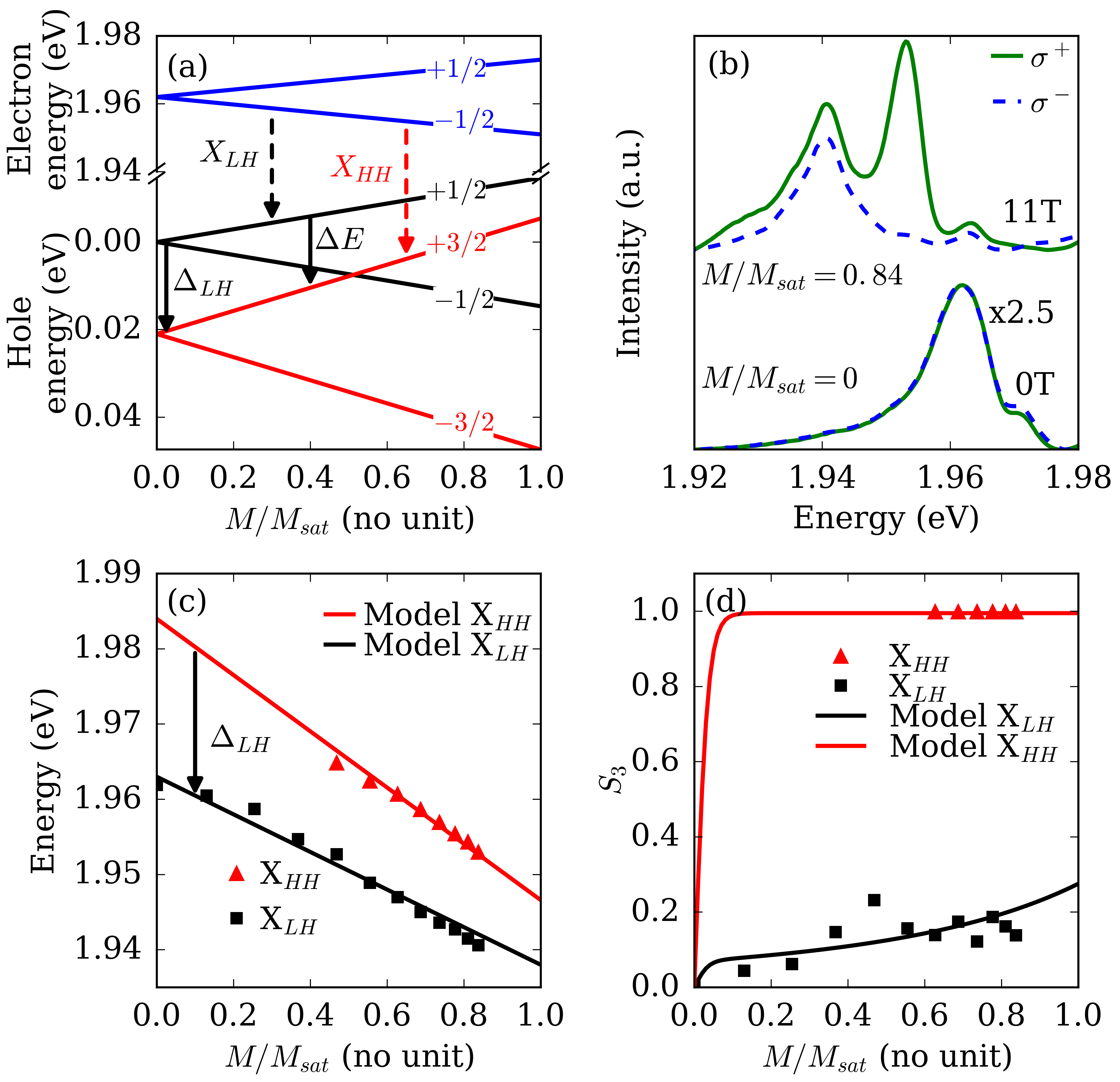
The analysis of the QD lines under magnetic field (Zeeman splitting and circular polarisation degree) provides another way to discriminate between LH and HH excitons. In our experiment, the magnetic field is applied along the NW axis (Faraday configuration). In non magnetic quantum dots with moderate exciton Landé factors, large magnetic fields are usually required in order to lift exciton spin manifold degeneracy. In (Cd,Mn)Te magnetic quantum dots, Mn atoms introduce localized spins randomly distributed in the dot. The large exchange interaction between Mn spins and confined carriers (electrons and holes) induces the so-called giant Zeeman splitting of the exciton lines at low temperature (effective Landé factor 100), which scales proportionally to the normalized quantum dot magnetic moment (see section I in the Supplemental Material [28]).[36] Even higher values are obtained with colloidal quantum dots.[37] In this case the strong anisotropy due to the wurtzite crystal structure enforces a heavy-hole character. Fig. 4(a) shows the Zeeman energy diagram of electrons and holes in an (Cd,Mn)Te/ZnTe QD with a 10% Mn concentration under a magnetic field applied along the axis and assuming . At low temperature and for magnetic fields larger than a fraction of , photo-carriers relax to the lowest energy levels ( for electrons and for holes). This induces both a red shift of the LH exciton line (black dashed arrow in Fig. 4(a), and a strong linear polarisation along ( polarisation), according to the optical selection rules recalled in Fig. 1(a). With the opposite assumption of a HH ground state, we would expect a polarisation.
In our experimental configuration, the magnetic field is applied along the NW axis which still stands along the optical axis (Faraday configuration), and the QD luminescence is collected over an angular range of NA = 0.4. Figure 4(b) shows the quantum dot emission spectra resolved in and polarisations for an applied magnetic field of and . The emission at zero field is dominated by the line at previously studied in far-field. At (corresponding to at ), the spectrum consists in two main lines at and . Both spectra present a weak satellite line at higher energy whose origin is unclear. The two lines are probably not related and a rather small Zeeman shift is observed (see Fig. 5 in Appendix A). It could be related to the luminescence from the substrate, or from parasitic growth which takes place between the nanowires. The Zeeman shift of the two main lines as a function of the QD magnetic moment is reported in Fig. 4(c). The first line, observed for all magnetic field values, presents a redshift proportional to . The shift at saturation is as expected for a LH exciton in a Cd0.9Mn0.1Te magnetic QD (see Appendix A). It shows very moderate circular polarisation imbalance, as expected for a LH emission which is ideally polarised. It confirms the LH exciton character of this line, as claimed by the analysis of farfield patterns in zero magnetic field. The second line is clearly present for fields larger than (). It is strongly polarised. It also redshifts proportionally to with a shift at saturation of . This value is definitely larger than the maximum possible LH Zeeman shift, whatever the Mn content, of . For these two reasons, we ascribe this line to the transition [red arrow in Fig. 4(a)] associated to the HH exciton. The saturation shift is lower than the value expected for a heavy-hole fully confined inside the dot (), suggesting a rather weak confinement of the HH excited state in the dot. At low field the behaviour of the line is complicated due to coupling to LH states. By extrapolating the Zeeman shift of the transition observed at high field down to we obtain a splitting . We want to stress here that the difference in the polarization of the two lines is a strong indication of the different nature of the hole involved in each transition, and rules out the possible emission from regions with different Mn content.
Information about the valence band mixing can be retrieved by a detailed analysis of the third Stokes parameter , plotted in Fig. 4(d) . The strong polarisation of the HH exciton line fully corresponds to the radiative recombination of a electron with a hole, and the selection rules given in Fig. 1(a). Surprisingly, one can note that the LH exciton line is also partially circularly polarised at large magnetic field (for ). This partial circular polarisation results from the hole mixing induced by the perturbation term (see Supplemental Material [28]). The black line in Fig. 4(d) give the theoretical variation of for the LH transition assuming a value of independent of the magnetic field and taking into account the ratio in collection efficiency of and polarised emission into the objective lens. The thermalization of the holes between the Zeeman levels has been added in order to get vanishing circular polarisation in zero field. Using the hole energy levels deduced from the Zeeman shifts of the exciton lines it yields 3%, in agreement with the the simulations of the zero field emission diagram. Due to the large value of , the mixing terms do not affect for the HH exciton at large magnetic field: the red line in Fig. 4(d) displays the circular polarisation expected for the heavy hole exciton.
IV Discussion
The polarized emission diagram of the ZnTe nanowire unambiguously reveals the HH character of the exciton, with a small mixing. This is expected [19] from the presence of the (Zn,Mg)Te shell with a smaller lattice parameter; the expected redshift was experimentally confirmed,[38, 29] and the heavy hole character was deduced from the giant Zeeman effect and the circular polarization observed with a (Zn,Mn)Te core. Using the composition profile obtained from Ref. 32 for a nanowire from the same sample, and analytical expressions of the strain-induced splitting, [19, 29] we expect and a ZnTe emission energy around in agreement with Fig. 2(a). This is consistent with the value deduced from the anisotropy of the giant Zeeman effect in (Zn,Mn,Te)/(Zn,Mg,Te) nanowires including a larger Mg content.[39] The mismatch between CdTe and ZnTe is opposite, so that we expect a LH character for a hole confined in a core-shell nanowire [19] or an elongated dot.[18] For InAs/InP, a local splitting is calculated [18] at the center of a cylinder-shape QD with an aspect ratio 2, but due to an inhomogeneous strain the HH state is above the ground state. In the present case, the aspect ratio is of the same order, the mismatch slightly larger, but the CdTe-ZnTe valence band offset is small so that another competition is expected with heavy-holes confined in the shell due to the shear strain around the dot.[19] A full calculation of is beyond the scope of this paper, but our measured value is of the right order or magnitude.
We measure a value of the mixing term meV. Larger values have been reported for self-assembled (Stranski-Krastanov) quantum dots.[25] Actually, an important feature is the symmetry of the principal axis, and switching from the to the orientation dramatically reduces in-plane asymmetry expected,[40] and measured.[41, 42] Our dots are embedded in nanowires grown along the axis. However the section of such nanowires easily feature some ellipticity, of the order of a few , easily detected on the shell [32] (although well beyond the resolution on the dot). A first evaluation of the strain in an elongated (aspect ratio ) ellipsoid with some in-plane ellipticity can be done using the Eshelby calculation: [43, 44] using the Bir-Pikus Hamiltonian, an ellipticity of gives the right order of magnitude for . Note that the same orientation of the ellipticity will change the phase of with the sign of the mismatch, as observed between the dot and the ZnTe core. Finally, writing the stiffness matrix with the axis as -axis [19] reveals that the presence of an in-plane shear () induces an axial shear stress, and hence a strain , of similar order of magnitude. This strain gives rise to a non-zero , which is not a tilt, but can be compensated by a tilt. Such a term is evidenced on the emission diagram of the quantum dot, while it is partly screened by guiding effect in the case of the ZnTe emission.
We have performed measurements on a set of NWQDs from the same sample mechanically deposited on a substrate. As they lie horizontally and close to a reflecting substrate which significantly disturbs the far-field radiation pattern, we could not perform the same characterization as for the as-grown wire. Nevertheless polarization studies reveal that the sample is actually close to the threshold between light-hole and heavy-hole ground state,[18] thus leading to a large dispersion in emission properties. A majority of the QDs () emit light linearly polarized along the NW axis, which in our system is a good indication of a LH ground state. The remaining emit light polarized perpendicularly to the NW axis, thus clearly indicating a HH character.
To conclude, complementary experiments on a single nanowire unambiguously demonstrate a LH exciton emission. They allow to evaluate the splitting as well as the valence band mixing parameters. The results are in agreement with the predictions of strain effects due to the presence of a shell around the wire. We demonstrate that valence band engineering through strain and confinement is possible using bottom up approach and semiconducting nanowire growth.
Acknowledgements.
We acknowledge the help of Institut Néel optical engineering team (CL, Fabrice Donatini). This work was supported by the French National Research Agency under contracts ANR-11-BS10-013, ANR-15-CE24-0029 and ANR-10-LABX-51-01, and Institut Universitaire de France.Appendix A Magneto-optical spectroscopy
Figure 5a displays photoluminescence spectra recorded at different values of the magnetic field applied along the nanowire axis. Only the extreme field values are plotted in Fig. 4a of the main text. Most salient features are the intense low energy line, which is present at zero field and displays a continuous red shift when increasing the intensity of the field. Fig. 5b, the position of this line is plotted for different values of the applied magnetic field and three values of the temperature (spectra of Fig. 5a, and spectra at two other temperatures, not shown), as a function of . The phenomenological parameter describes the antiferromagnetic interactions in Cd0.9Mn0.1Te, see above. The coincidence of the three sets of data confirms that the shift is due to the giant Zeeman effect, and follows a Brillouin function with a shift at saturation equal to (solid line). Note that this line exhibits only a small circular polarization. The second salient feature is the strongly -polarized line, visible at high field only. A weaker line is observed at high field, with a small Zeeman shift, which we did not identify (the nanowire is still on the substrate and parasitic growth takes place between the nanowires). Finally, the spectra at low fields appear as quite complex, but this is expected by the proximity of several hole sublevels at these field values (in particular, and which are expected to (anti)-cross at these field values, see Fig. 4b of the main text, and probably excited states of the hole).

(a) Photoluminescence spectra at K with a magnetic field applied along the nanowire axis, from to 11 T by steps of 1 T. The spectra at 0 and 11 T are displayed in Fig. 4a of main text. (b) Plot of the position of the low energy line as a function of )
Appendix B Theoretical background
B.1 Anisotropy of the holes
In a bulk semiconductor with the zinc-blende or diamond structure, the hole quadruplet is degenerate (representation of the cubic group). The presence of strain or confinement lifts this degeneracy. If a principal axis of symmetry exists, the hole Hamiltonian is usually written, in the basis quantized along this axis, as:
| (1) |
If is larger than and , the two Kramers doublet defined by this Hamiltonian are usually called light-hole and heavy-hole (even if these terms are not always justified), with the light-hole to heavy-hole energy splitting (the exact value of the splitting is ).
Two well known examples of this Hamiltonian are the Luttinger-Kohn Hamiltonian which describes the hole states in the vicinity of the valence band maximum, and the Bir-Pikus Hamiltonian which describes the coupling to a uniform strain.[45]
We want to stress here that this Hamiltonian is much more general: if the hole quadruplet is isolated, can be considered as a spin Hamiltonian, i.e., as an effective Hamiltonian operating within the quadruplet.[46] Some care must be taken when excited states have to be considered.[47]
Moreover, this effective Hamiltonian can be built as a linear combination of the successive powers of a pseudo-spin, with real coefficients. In the case of a quadruplet, powers of the operators up to 3 are enough, and in the absence of an applied magnetic field, only even powers have to be considered in order to fulfill the Kramers degeneracy. As a result, the most general spin Hamiltonian which describes the quadruplet at the top of the valence band can be written , where the vectorial operator is the (pseudo)-moment and is a real matrix. In addition, due to the commutation rules of , is symmetric. Note that the contribution of order zero to the spin Hamiltonian is redundant with the trace of ; both represent a rigid shift of the quadruplet, and a proper choice of the zero of energy allows us to set the trace of (hence that of ) to zero, as done in Eq. 1.
Using the matrices representing the second powers of in the , , and basis of the quadruplet, with the third axis as the quantization axis[45], the matrix elements of are
| (2) |
Expressions of the matrix elements of Eq. 1 (hence those of ) for the Luttinger-Kohn of Bir-Pikus Hamiltonian are generally expressed in the cubic basis.[27] However other axes can be chosen; for instance, in the case of a nanowire oriented along the axis, as in the present study, it is useful to choose this axis as the quantization axis.[19] If represents the coupling to a uniform strain (the Bir-Pikus Hamiltonian) for an isotropic system, is proportional to the axial shear strain , to the shear strain in the plane, , and to the combination of the shear strains in planes containing . However, it must be kept in mind that such a spin Hamiltonian is general and can describe other features governing the hole states, such as for instance the inhomogeneous strain expected in a quantum dot, or the effect of a confinement potential with a low symmetry.
Now, as the matrix is real and symmetric, a mere rotation makes it diagonal, with the three (real) eigenvalues on the diagonal. Using these eigenaxes (, , ), the spin Hamiltonian still writes , and it still develops as in Eq. 1, but Eq. 2 shows that now all matrix elements are real (including ), and :
| (3) |
with , and . If the axis is chosen so that is the eigenvalue with the largest absolute value, then ; the two Kramers doublet will be considered as light holes and heavy holes quantized along , with some mixing due to .
To sum up, the most general spin Hamiltonian describing the hole states is given by Eq. 1, where diagonal elements are real numbers but non-diagonal elements are complex numbers. Diagonalizing the corresponding matrix determines a rotation (i.e., three Euler angles) to a new set of axes where but also are real numbers and =0, Eq. 3.

As the principal axes of are those where the Hamiltonian is real with a vanishing , so that the hole states are most simple to write, it is useful to write the effect of a rotation on and . We apply to or the rotation defined by three Euler angles , see Fig. 6. It is particularly interesting - and technically simpler - to consider small values of , so that we keep only the first order in or . In this case, is the total angle of rotation around the axis (which has an effect only if the system does not feature circular symmetry, with non vanishing and different values of and ), while is the angle of the tilt and its direction. The rotation matrix in real space is
| (4) |
and the matrix elements of in the laboratory frame are obtained by a straightforward calculation of . is derived using Eq. 2, or calculated directly using the rotation , where the operator of rotation around (the tilt) is linearized. The result is quite simple. The hamiltonian assumes the form of Eq. 1, where:
| (5) |
These expressions have been used to fit the experimental data.
B.2 Geometrical visualizing of the anisotropy tensor
Since in the case of the Bir-Pikus Hamiltonian, the anisotropy matrix is proportional to the strain tensor (possibly weighted by the deformation potential parameters), it is often quite illuminating to pursue the analogy and to consider an ellipsoid defined in real space using the matrix , as an easy way to view the anisotropy within the hole quadruplet. One possibility is to consider a sphere of radius unity, to which we apply a strain , with an arbitrary scaling factor . If is larger than the largest eigenvalue of , the result is an ellipsoid which admits the , , eigen-axes of as principal axes, with a half-axis length along , and so on.
To first order in , the equation of such a solid is
| (6) |
where the ’s are the coordinates , , of an arbitrary frame.
The principal axes of the ellipsoid are those where is real with . A heavy-hole ground state implies , and the ellipsoid is oblate (flat). A light-hole ground state corresponds to a prolate (elongated) ellipsoid. The in-plane ellipticity is measured by . An example relevant for the present study is given in Fig. 6(a).
References
- [1] P. Michler, Science 290, 2282–2285 (2000).
- [2] A. Zrenner, E. Beham, S. Stufler, F. Findeis, M. Bichler, and G. Abstreiter, Nature 418, 612–614 (2002).
- [3] A. J. Shields, Nature Photon 1, 215 (2007).
- [4] C. Santori, M. Pelton, G. Solomon, Y. Dale, and Y. Yamamoto, Physical Review Letters 86, 1502–1505 (2001).
- [5] J. Claudon, J. Bleuse, N. S. Malik, M. Bazin, P. Jaffrennou, N. Gregersen, C. Sauvan, P. Lalanne, and J.-M. Gérard, Nature Photonics 4, 174 (2010).
- [6] C. Santori, D. Fattal, J. Vučković, G. S. Solomon, and Y. Yamamoto, Nature 419, 594–597 (2002).
- [7] N. Akopian, N. H. Lindner, E. Poem, Y. Berlatzky, J. Avron, D. Gershoni, B. D. Gerardot, and P. M. Petroff, Physical Review Letters 96, 130501 (2006).
- [8] A. Dousse, J. Suffczyński, A. Beveratos, O. Krebs, A. Lemaître, I. Sagnes, J. Bloch, P. Voisin, and P. Senellart, Nature 466, 217–220 (2010).
- [9] D. V. Bulaev and D. Loss, Physical Review Letters 95, 076805 (2005).
- [10] D. Heiss, S. Schaeck, H. Huebl, M. Bichler, G. Abstreiter, J. J. Finley, D. V. Bulaev, and D. Loss, Physical Review B 76, 241306 (2007).
- [11] D. Sleiter and W. F. Brinkman, Physical Review B 74, 153312 (2006).
- [12] D. E. Reiter, T. Kuhn, and V. M. Axt, Physical Review B 83, 155322 (2011).
- [13] H. Kosaka, T. Inagaki, Y. Rikitake, H. Imamura, Y. Mitsumori, and K. Edamatsu, Nature 457, 702–705 (2009).
- [14] G. Bester, S. Nair, and A. Zunger, Physical Review B 67, 161306 (2003).
- [15] L. He, G. Bester, and A. Zunger, Physical Review B 70, 235316 (2004).
- [16] Y. H. Huo, B. J. Witek, S. Kumar, J. R. Cardenas, J. X. Zhang, N. Akopian, R. Singh, E. Zallo, R. Grifone, D. Kriegner, and et al., Nat Phys 10, 46–51 (2013).
- [17] Y.-M. Niquet and D. C. Mojica, Physical Review B 77, 115316 (2008).
- [18] M. Zieliński, Phys. Rev. B 88, 115424 (2013).
- [19] D. Ferrand and J. Cibert, Eur. Phys. J. Appl. Phys. 67, 30403 (2014).
- [20] A. Lafuente-Sampietro, H. Boukari, and L. Besombes, Physical Review B 92, 081305(R) (2015).
- [21] H. E. Ruda and A. Shik, Journal of Applied Physics 100, 024314 (2006).
- [22] J. Bleuse, J. Claudon, M. Creasey, N. S. Malik, J.-M. Gérard, I. Maksymov, J.-P. Hugonin, and P. Lalanne, Physical Review Letters 106, 103601 (2011).
- [23] G. Grzela, R. Paniagua-Domínguez, T. Barten, Y. Fontana, J. A. Sánchez-Gil, and J. Gómez Rivas, Nano Lett. 12, 5481–5486 (2012).
- [24] G. Bulgarini, M. E. Reimer, M. Bouwes Bavinck, K. D. Jöns, D. Dalacu, P. J. Poole, E. P. A. M. Bakkers, and V. Zwiller, Nano Lett. 14, 4102–4106 (2014).
- [25] C. Tonin, R. Hostein, V. Voliotis, R. Grousson, A. Lemaitre, and A. Martinez, Phys. Rev. B 85, 155303 (2012).
- [26] T. Dietl, A. Haury, and Y. Merle d’Aubigné, Physical Review B 55, R3347–R3350 (1997).
- [27] G. L. Bir and G. Pikus, Symmetry and Strain-Induced Effects in Semiconductors, edited by N. Y. Wiley (Wiley, New York, 1974).
- [28] “See supplemental material at [url will be inserted by publisher] for details on the nanowires growth process and the experimental setups and information on the numerical procedure and theoretical developments.” .
- [29] A. Artioli, A., P. Rueda-Fonseca, P., P. Stepanov, P., E. Bellet-Amalric, M. Den Hertog, C. Bougerol, Y. Genuist, F. Donatini, R. André, R., G. Nogues, and et al., Applied Physics Letters 103, 222106 (2013).
- [30] P. Rueda-Fonseca, E. Bellet-Amalric, R. Vigliaturo, M. den Hertog, Y. Genuist, R. André, R., E. Robin, A. Artioli, P. Stepanov, D. Ferrand, and et al., Nano Lett. 14, 1877–1883 (2014).
- [31] P. Wojnar, M. Zielinski, E. Janik, W. Zaleszczyk, T. Wojciechowski, R. Wojnar, M. Szymura, L. Klopotowski, L. T. Baczewski, A. Pietruchik, and et al., Applied Physics Letters 104, 163111 (2014).
- [32] P. Rueda-Fonseca, E. Robin, E. Bellet-Amalric, M. Lopez-Haro, M. Den Hertog, Y. Genuist, R. André, A. Artioli, S. Tatarenko, D. Ferrand, and et al., Nano Lett. 16, 1637–1642 (2016).
- [33] P. Wojnar, J. Płachta, W. Zaleszczyk, S. Kret, A. M. Sanchez, R. Rudniewski, K. Raczkowska, M. Szymura, G. Karczewski, L. T. Baczewski, and et al., Nanoscale 8, 5720–5727 (2016).
- [34] P. Stepanov, Magneto-Optical Spectroscopy of Magnetic Semiconductor Nanostructures, Ph.D. thesis, Université Grenoble Alpes (2013).
- [35] W. H. McMaster, Rev. Mod. Phys. 33, 8–28 (1961).
- [36] T. Clément, D. Ferrand, L. Besombes, H. Boukari, and H. Mariette, Physical Review B 81, 155328 (2010).
- [37] R. Beaulac, L. Schneider, P. I. Archer, G. Bacher, and D. R. Gamelin, Science 325, 973–976 (2009).
- [38] P. Wojnar, E. Janik, L. T. Baczewski, S. Kret, E. Dynowska, T. Wojciechowski, J. Suffczyński, J. Papierska, P. Kossacki, G. Karczewski, J. Kossut, and T. Wojtowicz, Nano Lett. 12, 3404 (2012).
- [39] M. Szymura, P. Wojnar, Ł. Kłopotowski, J. Suffczyński, M. Goryca, T. Smole’nski, P. Kossacki, W. Zaleszczyk, T. Wojciechowski, G. Karczewski, and et al., Nano Lett. 15, 1972–1978 (2015).
- [40] R. Singh and G. Bester, Physical Review Letters 103, 063601 (2009).
- [41] T. Kuroda, T. Mano, N. Ha, H. Nakajima, H. Kumano, B. Urbaszek, M. Jo, M. Abbarchi, Y. Sakuma, K. Sakoda, and et al., Physical Review B 88, 041306 (2013).
- [42] G. Juska, V. Dimastrodonato, L. O. Mereni, A. Gocalinska, and E. Pelucchi, Nature Photon 7, 527–531 (2013).
- [43] J. D. Eshelby, Proceedings of the Royal Society A: Mathematical, Physical and Engineering Sciences 241, 376–396 (1957).
- [44] J. D. Eshelby, Proceedings of the Royal Society A: Mathematical, Physical and Engineering Sciences 252, 561–569 (1959).
- [45] G. Fishman, Semi-Conducteurs, les Bases de la Théorie k.p, edited by L. E. de l’Ecole Polytechnique (Les Editions de l’Ecole Polytechnique, 2010).
- [46] A. Abragam and B. Bleaney, Electron Paramagnetic Resonance of Transition Ions, edited by C. P. Oxford (Clarendon Press - Oxford, 1970).
- [47] J.-W. Luo, G. Bester, and A. Zunger, Physical Review B 92, 165301 (2015).