Inspiration or Preparation?
Explaining Creativity in Scientific Enterprise

At present, the most comprehensive dataset that captures information consumption in scientific enterprise is perhaps the web traffic generated by researchers, reflecting how they request and access online resources (e.g., online publication archives). Therefore, in our study, we used the Indiana University Click Dataset [19] (Click), which constitutes about 53.5 billion web requests initiated by researchers at Indiana University from 09/2006 to 05/2010. This anonymized dataset was collected by applying a Berkeley Packet Filter to the web traffic passing through the border router of Indiana University and matching all the traffic containing a HTTP GET request.

Each request consists of the following fields: $\langle$timestamp, requested url, referring url, agent, flag$\rangle$, where “agent” indicates whether the user agent was a browser or a bot, while “flag” indicates whether the request was generated inside or outside of Indiana University. All incoming or bot-generated requests have been filtered.

Meanwhile, to capture knowledge production in scientific enterprise, we used the Microsoft Academic Graph Dataset [25] (Mag). As of 11/06/2015, this dataset consists of 120.9 million papers published in 24,843 venues across all scientific fields.

In a nutshell, the Mag dataset is a web-scale entity graph comprising scientific publication records, citation relationships between publications, as well as their authors, author affiliations, publication venues, keywords and fields-of-study (i.e., topics). In particular, all the topics form a four-level hierarchy, with the highest and lowest levels corresponding to disciplines (e.g., “Computer science”) and specific subjects (e.g., “Decision tree”), respectively. Each keyword is associated with one topic in the hierarchy.

With a little abuse of notations, let ${\cal P}$ denote all the papers published in 2011 by Indiana University. We first measure the rarity and disconnect of all the reference pairs of ${\cal P}$, i.e., $\{(i,j)\in{\cal C}_{k}\}_{k\in{\cal P}}$. The results are shown in Figure 4.

Figure 4(a) shows the cumulative distribution of $(i,j)$’s rarity $r_{i,j}$. Note that around 60% pairs have zero co-citation before 2011. In Figure 4(b), we further measure the conditional distribution of $(i,j)$’s disconnect $d_{i,j}$ on its rarity $r_{i,j}$. The conditional distribution $Pr(d_{i,j}|r_{i,j})$ is fairly similar irrespective to varying $r_{i,j}$, implying that disconnect and rarity are two critical, but complementary factors of creativity. Then, according to Eqn.(1), we integrate $(i,j)$’s rarity and disconnect to compute its creativity score $\varphi_{i,j}$. As shown in Figure 4(c), the histogram of $\varphi_{i,j}$ roughly follows a lognormal distribution. It can be intuitively explained by that most reference pairs represent modestly “common” combinations, while both extremely “cliché” and “atypical” combinations are rare. Finally, we measure the creativity of papers in ${\cal P}$ by aggregating their reference pairs’ scores. We consider both average and median as the aggregation function $\ell(\cdot)$, with results depicted in Figure 4(d). Clearly, most of the papers show moderate creativity, which is consistent with the results reported in prior studies [26].

We further investigate the discipline-specific patterns of creativity measures. Figure 5(a)-(b) demonstrate the histogram of $(i,j)$’s creativity score $\varphi_{i,j}$ in the disciplines of Biology and Computer science respectively. Interestingly, one can observe that $\varphi_{i,j}$ roughly follows a lognormal distribution in Figure 5(a). Meanwhile, in Figure 5(b), $\varphi_{i,j}$ apparently follows a bimodal distribution, peaking at both low and high creativity scores. Such phenomena may be explained by that compared with Biology, Computer science is a relatively “engineering” discipline, featuring more frequent fusion of originally disconnected knowledge. As shown in Figure 5(c)-(d), this difference indeed leads to the disparate creativity distributions of papers published in these two disciplines: in general, the papers in Computer science demonstrate higher creativity.

We first directly compare reference set ${\cal C}_{t}$ against reading set ${\cal Q}_{t^{\prime}}$. In specific, we measure the paper-level dependency of ${\cal P}_{t}$ on ${\cal Q}_{t^{\prime}}$ by computing the Jaccard’s coefficient of ${\cal C}_{t}$ and ${\cal Q}_{t^{\prime}}$:

Figure 6(a) illustrates the paper-level dependency in our datasets. As $t$ varies from 2007 to 2014, we measure the dependency of ${\cal P}_{t}$ on ${\cal Q}_{t^{\prime}}$ for $t^{\prime}(t^{\prime}<t)$ ranging from 2006 to 2009.

It is observed that this paper-level dependency demonstrates interesting temporal dynamics. First, given reading set ${\cal Q}_{t^{\prime}}$ (i.e., fixed $t^{\prime}$), the dependency of ${\cal P}_{t}$ on ${\cal Q}_{t^{\prime}}$ decreases as $t$ grows, implying that the impact of ${\cal Q}_{t^{\prime}}$ gradually decays over time. Second, for given publication set ${\cal P}_{t}$ (i.e., fixed $t$), its dependency on ${\cal Q}_{t^{\prime}}$ increases with $t^{\prime}$, implying that more recent reading papers exert more influence over future publications.

We then examine the dependency of publication set ${\cal P}_{t}$ on reading set ${\cal Q}_{t^{\prime}}$ at the topic level.

In specific, following the definition of topic disconnect in Eqn.(4), we compute the topic-level dependency of ${\cal P}_{t}$ on ${\cal Q}_{t^{\prime}}$ as the average “connectedness” of papers in ${\cal P}_{t}$ and ${\cal Q}_{t^{\prime}}$:

The measurement results are illustrated in Figure 6(b). We have the following observations.

The topic-level dependency shows pattens similar to the paper-level dependency: (i) the impact of reading papers over future publications decays over time; (ii) more recent reading papers exert stronger influence. Nevertheless, compared with the paper-level dependency, the topic-level dependency seems less “stratified” in that adjacent years show more resemble patterns. For instance, the dependency with respect to the reading papers in 2006 and 2007 shows strong similarity. Such phenomena can be explained by that authors’ interests in particular topics are more stable than their interests in concrete papers.

To answer this question, we introduce a mathematical model to quantify the impact of information consumption in creative processes. To motivate the rationale behind our model, let us consider the following concrete example of three papers by three disjoint groups of authors.

• • –

    $i$: “Fast algorithms for mining association rules”. R. Agrawal and R. Srikant. VLDB ’94.

  • –

    $x$: “Frequent subgraph discovery”. M. Kuramochi and G. Karypis. ICDM ’01.

  • –

    $j$: “SPIN: mining maximal frequent subgraphs from graph databases”. J. Huan, W. Wang, J. Prins and J. Yang. KDD ’04.

Here paper $j$ differs from $i$ significantly. However, after reading paper $x$, one is probably able to draw the connection from $i$ to $j$ as “frequent pattern” $\rightarrow$ “frequent subgraph pattern” $\rightarrow$ “maximal frequent subgraph pattern”. Informally, reading $x$ offers the opportunity to bridge the knowledge gap between $i$ and $j$.

We capture this intuition using the metric of creativity score defined in Eqn.(1). The term $\varphi_{i,j}$ can be interpreted as the “difficulty” of connecting $(i,j)$, while the exposure to $x$ may potentially reduce this difficulty. That is, instead of directly connecting $(i,j)$, one may now first connect $i$ to $x$, and then link $x$ to $j$, as illustrated in Figure 7.

Formally, we introduce a metric to describe the impact of paper $x$ on the creativity required to connect $(i,j)$:

where the term $\max\left(\varphi_{i,k},\varphi_{k,j}\right)$ represents the difficulty of connecting $(i,x)$ and $(x,j)$.

Note that this definition can be generalized to the case that $n$ papers ${\bm{x}}=\{x_{1},x_{2},\ldots,x_{n}\}$ collectively bridge the gap of $(i,j)$ by creating an $n$-hop “path” between them. Let $\varphi_{\bm{x}}=\max_{l=1}^{n-1}\varphi_{x_{l},x_{l+1}}$. We may define the impact of $\bm{x}$ to $(i,j)$ as: $\Delta^{i,j}_{\bm{x}}=\varphi_{i,j}-\min\left(\varphi_{i,j},\max\left(\varphi_{i,x_{1}},\varphi_{\bm{x}},\varphi_{x_{n},j}\right)\right)$. Due to space limitations, in the following discussion we focus on the case of $n=1$.

We are now ready to perform an anatomy of the creativity $\varphi_{i,j}$ required to connect the knowledge represented by two papers $(i,j)$. For simplicity, consider the case that during this creative process, the authors read a single paper $x$. We divide $\varphi_{i,j}$ into two complementary parts.

• • –

    “Preparation” - the marginal reduction in the difficulty of connecting $(i,j)$, due to the authors’ reading, which is quantified by $\Delta^{i,j}_{x}$.

  • –

    “Inspiration” - the part of creativity that cannot be explained by the authors’ reading, which is quantified by $(\varphi_{i,j}-\Delta^{i,j}_{x})$.

Since a given paper blends the knowledge in all its references, a dichomatic theory naturally follows. That is, a paper’s creativity reflects a superimpose of both effects:

$$\mathrm{𝐂𝐫𝐞𝐚𝐭𝐢𝐯𝐢𝐭𝐢𝐲}=\mathrm{𝐏𝐫𝐞𝐩𝐚𝐫𝐚𝐭𝐢𝐨𝐧}+\mathrm{𝐈𝐧𝐬𝐩𝐢𝐫𝐚𝐭𝐢𝐨𝐧}$$

Formally, consider a paper $k$ with ${\cal C}_{k}$ as its reference set. Assume that $k$’s authors have read a set of papers ${\cal Q}$ during their creative process. As given in Eqn.(2), $k$’s overall creativity is assessed by: $\phi_{k}=\ell(\{\varphi_{i,j}\}_{i,j\in{\cal C}_{k}})$. For each pair $i,j\in{\cal C}_{k}$, we identify a reading paper in ${\cal Q}$ that maximally impacts $\varphi_{i,j}$ and compute its impact as:

Thus, after discounting the preparation quantity embodied in ${\cal Q}$, the inspiration of $k$, $\chi_{k}$, is measured as:

while the preparation quantity $\psi_{k}$ is computed as the difference of creativity and inspiration measures:

In the creativity theory above, the definition of ${\cal Q}$ is critical for accurately quantifying preparation and inspiration. While one may regard all the papers read by given authors in the past as ${\cal Q}$, this simplification ignores the temporal dynamics of information production-consumption dependency observed in § 5.1, resulting in an overestimation of preparation quantities. Here we will address this issue.

It is extremely difficult to directly assess the temporal dynamics of a reading paper $x$’s impact over a future publishing paper $k$. However, by studying in general how authors access papers in the intersection of reference and reading sets (i.e., ${\cal C}_{k}\cap{\cal Q}$), we are able to build a surrogate temporal dynamics model.

Specifically, for $x\in{\cal C}_{k}\cap{\cal Q}$, we examine $x$’s reading time ($t^{r}_{x}$) and $k$’s publishing time ($t^{p}_{k}$). The difference ($\tau^{r}_{x,k}=t^{p}_{k}-t^{r}_{x}$) reflects the temporal interval between information consumption and knowledge production. Figure 8(a) shows that this interval follows a log-log distribution, which is consistent with the studies on papers’ “aging” phenomena [10]. Let $Pr(\tau)$ represent this distribution. By discretizing and normalizing $Pr(\tau)$, we compute the probability that a reading paper influences a future paper published $\Delta t$ years later, i.e., $m(\Delta t)=\int_{\tau=\Delta t}^{+\infty}Pr(\tau)\textrm{d}\tau$.

Putting everything together, Algorithm 1 sketches how to compute a given paper $k$’s preparation and inspiration quantities. For each reference pair $i,j\in{\cal C}_{k}$, the papers in reading set ${\cal Q}$ are ranked according to their impact to the creativity score of $(i,j)$; the current top one $x^{*}$ is picked with probability $m(\tau^{r}_{x^{*},k})$; if $x^{*}$ is not picked, it moves to the next most impactful one and repeats this process; finally, $k$’s preparation and inspiration measures are computed by aggregating the creativity scores of all reference pairs.

Applying Algorithm 1, we first assess the preparation and inspiration quantities of papers published in 2011 (similar phenomena are observed in other years). In particular, we examine the papers in the disciplines of Biology and Computer science separately.

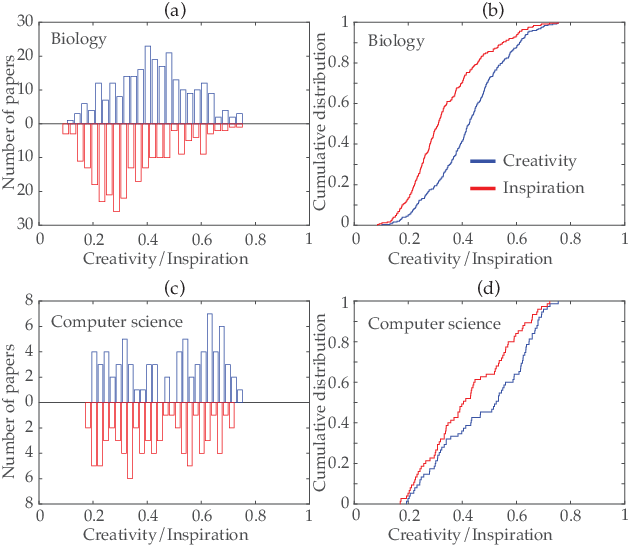
Figure 9 contrasts a paper $k$’s overall creativity $\phi_{k}$ and inspiration $\chi_{k}$. Specifically, Figure 9(a)-(c) show the histograms of $\phi_{k}$ and $\chi_{k}$ regarding the papers in Biology and Computer science, respectively; Figure 9(b)-(d) further compare their cumulative distributions. It is observed in both cases, $\psi_{k}$ accounts for a sizable portion of $\phi_{k}$. Table 1 summarizes the impact of $\psi_{k}$. We examine the papers whose creativity measures drop after the preparation is taken into account. For example, of about 59.0% papers across all scientific fields, 25.7% of their creativity can be explained by information consumed by their authors. Also interestingly, the quantity of preparation varies with specific disciplines: it counts for 21.9% and 29.2% of creativity in the disciplines of Computer science and Biology, respectively. This variance may be explained by that in a more established discipline as Biology, authors need to ground their research in existing work more profoundly.

We further explore the practical use of this creativity theory. Here we report one concrete case.

The target paper $k$: “Engaging online learners: the impact of web-based learning technology on college student engagement” cites two papers $i$: “A comprehensive look at online student support services for distance learners” and $j$: “Do computers enhance or detract from student learning?”. The reading paper $x$: “The convergent and discriminant validity of NSSE scalelet scores” reduces $\varphi_{i,j}$ from 0.661 to 0.495.

At a first glance, $x$ is not relevant to either $i$ or $j$. Yet, after manually examining the full text of these papers, one may notice the following connection: to build an online learning environment ($i$’s knowledge), it is critical to effectively assess student engagement in this new environment ($j$’s knowledge), while $x$ indeed provides a metric to evaluate student engagement.

Finally, we investigate the relationships of preparation and inspiration with other important metrics of scientific work. In particular, we focus on a paper’s citation count, the de facto metric of its long-term impact [28, 3, 9, 18].

Figure 10 plots the correlation of a paper $k$’s preparation $\psi_{k}$ and inspiration $\chi_{k}$ with its citation count $c_{k}$. Again, we examine papers in the disciplines of Biology and Computer science separately. In both cases, $c_{k}$ is positivity correlated with $\psi_{k}$, implying that a paper grounded deeper into exiting work is better received by the research community. More interesting is the correlation of $c_{k}$ and $\chi_{k}$: it is positive in the case of Computer science, yet slightly negative in the case of Biology. This may be explained by that as a younger and more vibrant discipline, the Computer science community tends to be more welcoming to radical ideas that blend previously disconnected knowledge.

Clearly, the creativity, preparation and inspiration metrics provide a new perspective to assess scientific publications’ merits. We envision that in synergy with other metrics (e.g., citation count), they may lead to more comprehensive understanding of long-term impact of scientific work.

Let $R(k,{\cal A})=\ell(\{\varphi_{i,j}\}_{i,j\in{\cal C}_{k}})-\ell(\{\varphi_{i,j}-\Delta^{i,j}_{{\cal A}}\}_{i,j\in{\cal C}_{k}})$. We update the objective function as:

where $\lambda_{k}$ is paper $k$’s weight, indicating its importance, with $\forall k\in{\cal P},\lambda_{k}\geq 0$ and $\sum_{k\in{\cal P}}\lambda_{k}=1$.

Under this multi-criterion setting, there may be cases that two solutions ${\cal A},{\cal A}^{\prime}$ are incompatible, i.e., $R(k,{\cal A})>R(k,{\cal A}^{\prime})$ while $R(k^{\prime},{\cal A})<R(k^{\prime},{\cal A}^{\prime})$. Instead of looking for the optimal solution, we resort to finding a Pareto-optimal solution [2]. A solution ${\cal A}$ is Pareto-optimal if no other solution ${\cal A}^{\prime}$ satisfies that (i) $R(k,{\cal A}^{\prime})\geq R(k,{\cal A})$ for all $k\in{\cal P}$ and $k\neq k^{\prime}$, and (ii) $R(k^{\prime},{\cal A}^{\prime})>R(k^{\prime},{\cal A})$ for a specific $k^{\prime}\in{\cal P}$.

As $R(\cdot)$ is a non-negative linear combination of submodular functions, any solution that maximizes $R(\cdot)$ is guaranteed to be Pareto-optimal [2]. Moreover, since the submodularity is closed under the non-negative linear combinations, Algorithm 2 can be readily applied.

Furthermore, we take into account the temporal dynamics of information production-consumption dependency (cf. § 5.2). To build the temporal dynamics model, for $x\in{\cal C}_{k}\cap{\cal Q}$, we examine $x$’s publishing time ($t^{p}_{x}$) and $k$’s publishing time ($t^{p}_{k}$). The difference ($\tau_{x,k}^{p}=t^{p}_{k}-t^{p}_{x}$) reflects the temporal gap between $x$ and $k$’s publishing. Figure 8(b) shows that this interval fits a log-log distribution, denoted by $Pr(\tau)$. By discretizing and normalizing $Pr(\tau)$, we compute the probability that a paper published $\Delta t$ years ago influences a current paper, i.e., $m(\Delta t)=\int_{\tau=\Delta t}^{+\infty}Pr(\tau)\textrm{d}\tau$. Similar to Algorithm 1, we incorporate this temporal dynamics into Algorithm 2 (line 7-9). We omit the details due to space limitations.

References

- [1] R. Agrawal and R. Srikant. Fast algorithms for mining association rules in large databases. In Proceedings of the 20th International Conference on Very Large Data Bases, VLDB ’94, 1994.
- [2] S. Boyd and L. Vandenberghe. Convex Optimization. Cambridge University Press, New York, NY, USA, 2004.
- [3] J. Cheng, L. Adamic, P. A. Dow, J. M. Kleinberg, and J. Leskovec. Can cascades be predicted? In Proceedings of the 23rd International Conference on World Wide Web, WWW ’14, 2014.
- [4] R. Collins. The Sociology of Philosophies: A Global Theory of Intellectual Change. Belknap Press of Harvard University Press, 1998.
- [5] S. Colton. Creativity versus the perception of creativity in computational systems. In AAAI Spring Symposium: Creative Intelligent Systems’08, 2008.
- [6] M. Csikszentmihalyi. Creativity-flow and the psychology of discovery and invention. Harper perennial, 1996.
- [7] T. De Smedt. Modeling Creativity: Case Studies in Python. ArXiv e-prints, 2014.
- [8] S. Doboli, F. Zhao, and A. Doboli. New measures for evaluating creativity in scientific publications. ArXiv e-prints, 2014.
- [9] Y. Dong, R. A. Johnson, and N. V. Chawla. Will this paper increase your h-index?: Scientific impact prediction. In Proceedings of the Eighth ACM International Conference on Web Search and Data Mining, WSDM ’15, 2015.
- [10] S. N. Dorogovtsev and J. F. F. Mendes. Evolution of Networks: From Biological Nets to the Internet and WWW (Physics). Oxford University Press, Inc., New York, NY, USA, 2003.
- [11] J. A. Evans and J. G. Foster. Metaknowledge. Science, 331(6018):721–725, 2011.
- [12] L. Fleming. Recombinant uncertainty in technological search. Management Science, 47(1):117–132, 2001.
- [13] L. Gabora and A. Saab. Creative interference and states of potentiality in analogy problem solving. In Proceedings of the Annual Meeting of the Cognitive Science Society, COGSCI ’13, 2013.
- [14] M. R. Guevara, D. Hartmann, M. Aristarán, M. Mendoza, and C. A. Hidalgo. The Research Space: using the career paths of scholars to predict the evolution of the research output of individuals, institutions, and nations. ArXiv e-prints, 2016.
- [15] B. F. Jones, S. Wuchty, and B. Uzzi. Multi-university research teams: Shifting impact, geography, and stratification in science. Science, 322(5905):1259–1262, 2008.
- [16] D. Kim, D. Burkhardt Cerigo, H. Jeong, and H. Youn. Technological novelty profile and invention’s future impact. ArXiv e-prints, 2015.
- [17] A. Koestler. The Act of Creation. Arkana, 1964.
- [18] L. Li and H. Tong. The child is father of the man: Foresee the success at the early stage. In Proceedings of the 21th ACM SIGKDD International Conference on Knowledge Discovery and Data Mining, KDD ’15, 2015.
- [19] M. Meiss, F. Menczer, S. Fortunato, A. Flammini, and A. Vespignani. Ranking web sites with real user traffic. In Proc. First ACM International Conference on Web Search and Data Mining (WSDM), 2008.
- [20] G. L. Nemhauser, L. A. Wolsey, and M. L. Fisher. An analysis of approximations for maximizing submodular set functions—i. Mathematical Programming, 14(1):265–294, 1978.
- [21] Plato. The republic, Book X.
- [22] M. Rosvall and C. T. Bergstrom. Maps of random walks on complex networks reveal community structure. Proceedings of the National Academy of Sciences, 105(4):1118–1123, 2008.
- [23] R. Saunders and J. S. Gero. Artificial creativity: A synthetic approach to the study of creative behaviour. In Computational and Cognitive Models of Creative Design V, 2001.
- [24] W. Shadish and S. Fuller. The social psychology of science. Guilford Press, 1994.
- [25] A. Sinha, Z. Shen, Y. Song, H. Ma, D. Eide, B.-J. P. Hsu, and K. Wang. An overview of microsoft academic service (mas) and applications. In Proceedings of the 24th International Conference on World Wide Web, WWW ’15 Companion, 2015.
- [26] B. Uzzi, S. Mukherjee, M. Stringer, and B. Jones. Atypical combinations and scientific impact. Science, 342(6157):468–472, 2013.
- [27] T. Veale and Y. Hao. Learning to understand figurative language: From similes to metaphors to irony. In Proceedings of the Annual Meeting of the Cognitive Science Society, COGSCI ’07, 2007.
- [28] D. Wang, C. Song, and A.-L. Barabási. Quantifying long-term scientific impact. Science, 342(6154):127–132, 2013.
- [29] M. Weitzman. Recombinant growth. Quarterly Journal of Economics, 113(2):331–360, 1998.
- [30] G. A. Wiggins. A preliminary framework for description, analysis and comparison of creative systems. Know.-Based Syst., 19(7):449–458, 2006.