Nonreciprocal microwave signal processing with a Field-Programmable Josephson Amplifier

We start with the first building block: frequency conversion between two modes, here chosen to be $a$ and $b$. We modulate the flux through the SQUID with a pump at a frequency $\omega_{ab}^{p}\approx\left\lvert\omega_{b}-\omega_{a}\right\rvert$. An input signal of amplitude $a_{\text{in}}$, driving the mode amplitude $a$ at a frequency $\omega_{a}^{\text{s}}$, is coupled to the mode amplitude $b$, leading to an output signal of amplitude $b_{\text{out}}$ at a frequency $\omega_{b}^{\text{s}}=\omega_{a}^{\text{s}}+\omega_{ab}^{p}$, and vice versa (see Fig. 2(a)). The EoMs in the signal frame reduce to

with $\Delta_{j}=(\omega_{j}^{\text{s}}-\omega_{j})/\kappa_{j}+i/2$ the normalized detuning for mode ${j}$ and $\beta_{ab}=|g_{ab}|e^{i\phi_{ab}}/(2\sqrt{\kappa_{a}\kappa_{b}})$ the normalized coupling between the mode amplitudes $a$ and $b$. Importantly, this coupling term is complex, with its phase $\phi_{ab}$ and amplitude $\left\lvert g_{ab}\right\rvert$ inherited from the pump. We show in Fig. 2(b) a graph representation of the EoMs in Eq. 2, where vertices represent the mode amplitude and arrows represent the detuning and coupling terms. In the ideal resonant case, defined as $\omega_{ab}^{p}=\left\lvert\omega_{b}-\omega_{a}\right\rvert$ and $\omega_{j}^{\text{s}}=\omega_{j}$, and neglecting internal loss, $\kappa_{j}^{\text{int}}=0$, the scattering matrix $\mathbf{S}$ for the system is

Close examination of the scattering matrix reveals that unity transmission coincides with impedance matching (zero reflection) at $\left\lvert\beta_{ab}\right\rvert=1/2$, and the corresponding signal flow diagram [32] is shown in Fig. 2(c). We note here that $S_{ba}=-S_{ab}^{*}$, naïvely providing gyration. While this will be crucial later for establishing directionality, on its own this is not unconditionally nonreciprocal due to an ambiguity in the reference frame when describing scattering between two different frequency modes[30, 15, 16].

The measured scattering parameters in our device are shown in Fig. 2(d) as a function of the detuning $\delta_{j}=\omega_{j}^{\text{s}}-\omega_{j}$. We fit the measured response using the full solutions of Eq. 2, finding very good agreement with the data. In particular, we measure only $0.5~\text{dB}$ of insertion loss, fully captured by including the internal loss of the resonators so that $\left\lvert S_{ba}\right\rvert^{2}=\kappa_{a}^{\text{ext}}\kappa_{b}^{\text{ext}}/\kappa_{a}\kappa_{b}$ (see Appendix B). The circuit is well matched, with $30~\text{dB}$ of return loss. The bandwidth of conversion is $\sqrt{\kappa_{a}\kappa_{b}}/2\pi\approx 30~\text{MHz}$.

We now describe the second building block: amplification between two modes, here chosen to be $a$ and $b$. We modulate the flux through the SQUID with a pump at the sum frequency $\omega_{ab}^{p}\approx\omega_{b}+\omega_{a}$. An input signal at a frequency $\omega_{a}^{\text{s}}$ is amplified and generates an idler at $-\omega_{b}^{\text{s}}=\omega_{a}^{\text{s}}-\omega_{ab}^{p}$ (see Fig. 3(a)). In contrast with the frequency conversion case in Eq. 2 the dynamics of the mode amplitude $a$ are now coupled to the conjugated mode amplitude $b^{*}$ and the EoMs in the signal frame reduce to

with $\Delta_{j}=(\omega_{j}^{\text{s}}-\omega_{j})/\kappa_{j}+i/2$ and $\beta_{ab}=|g_{ab}|e^{-i\phi_{ab}}/(2\sqrt{\kappa_{a}\kappa_{b}})$. Again, when comparing with the frequency conversion case, one can notice the sign change for the detuning term and the coupling term in the equation for $b^{*}$. These subtle differences lead to a very different scattering matrix $\mathbf{S}$, which in the ideal resonant case ($\omega_{ab}^{p}=\omega_{b}+\omega_{a}$ and $\omega_{j}^{\text{s}}=\omega_{j}$), and neglecting internal loss ($\kappa_{j}^{\text{int}}=0$), is

Close examination of the scattering matrix in Eq. 5 reveals a divergence for $\left\lvert\beta_{ab}\right\rvert=1/2$, in stark contrast with the frequency conversion case (Eq. 3). In the limit $\left\lvert\beta_{ab}\right\rvert\rightarrow 1/2^{-}$ each scattering parameter has an amplitude gain related to $\sqrt{G}\approx 2/(1-4\left\lvert\beta_{ab}\right\rvert^{2})$, and the full signal flow is shown in Fig. 3(c). As in the frequency conversion case, note that $S_{ba}=S_{ab}^{*}$. In Fig. 3(d) we show the measured scattering parameters for various values of $\left\lvert\beta_{ab}\right\rvert$, i.e., for various pump powers. As $\left\lvert\beta_{ab}\right\rvert$ increases, so does the gain, at the expense of a typical reduction in linewidth [33]. Good agreement is found with a fit to the solutions of Eq. 4.

The noise performance of the amplifier is shown in Fig. 3(e). In a separate experiment we calibrated an upper bound for the system added noise of the measurement setup at the reference plane of the FPJA, as explained in detail in Appendix C. When the FPJA is operated as an amplifier we measure a noise rise, and the knowledge of the noise floor in photon units allows us to extract the system added noise referred to the input of the FPJA. For $\left\lvert\beta_{ab}\right\rvert=0$, we observe a slight degradation of the system added noise due to the internal loss of the resonators, up to $n_{\text{add}}\approx 40~\text{photons}$ at $\omega_{a}$ and $n_{\text{add}}\approx 30~\text{photons}$ at $\omega_{b}$. As the gain increases, the noise contribution of the measurement chain is overwhelmed and the system added noise decreases, down to $n_{\text{add}}\approx 1.0\pm 0.1~\text{photons}$ at $\omega_{a}$ and $\omega_{b}$, approaching the Standard Quantum Limit (SQL) of $n_{\text{add}}^{\text{SQL}}=0.5$. The system added noise plateaus at high gain, remaining slightly above the SQL. This could originate from excess thermal population of the resonators, potential excess loss in the FPJA packaging or simply from an offset in the reference plane of the noise calibration.

By connecting all three resonators via frequency conversion, we can build the first nontrivial mode of operation: the circulator. Using three pumps, we modulate the flux through the SQUID at the difference frequencies $\omega_{jk}\approx\left\lvert\omega_{j}-\omega_{k}\right\rvert$, where ${j},{k}\in\{{a,b,c}\}$, satisfying the condition $\omega_{ab}^{p}+\omega_{bc}^{p}=\omega_{ac}^{p}$ (see Fig. 4(a)). Effectively, this forms a closed loop in frequency space connecting input and output signals at $\omega_{j}^{\text{s}}$, where ${j}\in\{{a,b,c}\}$. The EoMs in the signal frame reduce to:

with $\Delta_{j}=(\omega_{j}^{\text{s}}-\omega_{j})/\kappa_{j}+i/2$ and $\beta_{jk}=|g_{jk}|e^{i\phi_{jk}}/(2\sqrt{\kappa_{j}\kappa_{k}})$, where ${j},{k}\in\{{a,b,c}\}$. The graph representation of this equation is shown in Fig. 4(b). This loop topology is at the heart of the nonreciprocal behavior of this mode of operation. Indeed, by closing this loop we build an interferometer, where the phase shift in each arm is direction dependent. The interference is controlled by the loop phase $\phi_{\mathrm{loop}}=\phi_{ab}+\phi_{bc}-\phi_{ac}$, where $\phi_{jk}$ is the phase of the pump connecting modes ${j}$ and ${k}$. In the ideal resonant case $\omega_{jk}=\left\lvert\omega_{j}-\omega_{k}\right\rvert$ and $\omega_{j}^{\text{s}}=\omega_{j}$, neglecting internal loss, tuning each coupling strength to produce ideal frequency conversion ($\left\lvert\beta_{jk}\right\rvert=1/2$), and for $\phi_{\mathrm{loop}}=-\pi/2$, the scattering matrix $\mathbf{S}$ for the system is

In this case the system is matched, with $\left\lvert S_{jj}\right\rvert=0$, and nonreciprocal, $\left\lvert S_{jk}\right\rvert\neq\left\lvert S_{kj}\right\rvert$, corresponding to the signal flow diagram in Fig. 4(c). An input signal in mode $a$ circulates to mode $b$ then $c$. The direction of circulation is controlled by the loop phase and can be reversed by setting $\phi_{\mathrm{loop}}=\pi/2$.

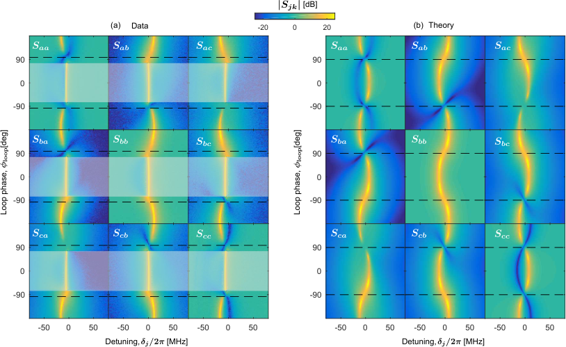
Experimentally we start by tuning the pumps to produce ideal frequency conversion between each pair of modes separately, and then simultaneously turn on all three pumps. The measured scattering parameters for $\phi_{\mathrm{loop}}=-\pi/2$ are shown in Fig. 4(d). The full dependence with the loop phase $\phi_{\mathrm{loop}}$ is shown in Fig. 8. Very good agreement is obtained with solutions of Eq. 6. With return loss exceeding 20 dB the device exhibits excellent impedance match at all three modes. We measure a transmission efficiency of more than $-0.5~\mathrm{dB}$ and an isolation exceeding $20~\text{dB}$ over a $6~\text{MHz}$ bandwidth. A transmission efficiency of more than $-1~\mathrm{dB}$ and an isolation exceeding $10~\text{dB}$ is maintained over a $60~\text{MHz}$ bandwidth.

When operated as a two-mode amplifier the FPJA is non-directional (see Fig. 3), and requires a circulator to separate the input and output signals. In this section we circumvent this requirement by operating the FPJA as a directional amplifier. Using three pumps, we modulate the flux through the SQUID at frequencies $\omega_{ac}^{p}\approx\omega_{c}-\omega_{a}$, $\omega_{ab}^{p}\approx\omega_{b}+\omega_{a}$ and $\omega_{bc}^{p}\approx\omega_{c}+\omega_{b}$, satisfying the overall loop closure condition $\omega_{ac}^{p}+\omega_{ab}^{p}=\omega_{bc}^{p}$ (see Fig. 5(a)). This corresponds to simultaneously connecting modes $a$ and $c$ via frequency conversion, while connecting modes $a$ and $b$ and modes $b$ and $c$ via amplification, forming a loop in frequency space. The resulting EoMs are

The graph representation of these EoMs is shown in Fig. 5(b). Similarly to the circulator case, the loop phase $\phi_{\mathrm{loop}}=\phi_{ab}+\phi_{bc}+\phi_{ac}$ controls the direction of the amplification. In the ideal resonant case, neglecting internal loss, tuning the coupling strength to produce ideal frequency conversion between modes $a$ and $c$, $\left\lvert\beta_{jk}\right\rvert=1/2$, for symmetric amplification coupling strength $\left\lvert\beta_{ab}\right\rvert=\left\lvert\beta_{bc}\right\rvert$, and for $\phi_{\mathrm{loop}}=-\pi/2$, the scattering matrix $\mathbf{S}$ is

where $\sqrt{G}=\left(1+4\left\lvert\beta_{ab}\right\rvert^{2}\right)/\left(1-4\left\lvert\beta_{ab}\right\rvert^{2}\right)$. In this configuration, mode $a$ serves as the input port and is impedance matched (no reflection). An input signal is amplified toward both output modes $b$ and $c$. The amplified signal at each output is added to the amplified vacuum seeded into mode $b$, resulting in the same minimum system added noise as for a standard two-mode amplifier. Finally, vacuum noise seeded into mode $c$ is routed to mode $a$ with unity gain. The measured scattering parameters for $\phi_{\mathrm{loop}}=\pi/2$ are shown in Fig. 5(d). The full dependence with the loop phase $\phi_{\mathrm{loop}}$ is shown in Fig. 9. Good agreement is obtained with numerical solutions of Eq. 8. We obtain a forward gain of $18~\text{dB}$ while maintaining good impedance matching (return loss in excess of $10~\text{dB}$) and isolation (in excess of $8~\text{dB}$). The noise performances are shown in Fig. 5 (e), (f) and (g), corresponding to the respective output of mode $a$, $b$ and $c$. The system added noise measured at the output of mode $b$ and $c$, referred to the input of mode $a$, approaches the quantum limit with $n_{\text{add}}\approx 1.1\pm 0.1~\text{photons}$. Moreover, due to the directionality of the amplifier, we do not observe any noise rise at the output of mode $a$, and therefore do not expect any backaction on a future DUT —a crucial property for the integrated measurement of a microwave quantum system.

The Hamiltonian for a driven harmonic oscillator with resonant frequency $\omega_{a}$ and loss rate $\kappa_{a}$, after tracing over bath modes in the rotating wave approximation, is

where $\kappa_{a}^{\text{ext}}$ is the external coupling to the drive port, and $\hat{a}$ and $\hat{a}_{\text{in}}$ are the time-dependent annihilation operators for the internal mode and input drive respectively. To simplify the notation we choose (1) to include the loss as an imaginary component of the resonant frequency, making the Hamiltonian non-Hermitian and (2) to have the phase quadrature of the drive coupled to the amplitude quadrature of the internal mode. Note that to preserve quantum commutators, Eq. 10 needs an extra noise input term proportional to $\sqrt{\kappa_{a}^{\text{int}}}$ so that $\kappa_{a}=\kappa_{a}^{\text{ext}}+\kappa_{a}^{\text{int}}$ (see section B.4).

The Heisenberg-Langevin EoM is $\dot{\hat{a}}=-i\left[\hat{a},\hat{\mathcal{H}}/\hbar\right]$. To analyze the EoM, we consider an input signal at the signal frequency $\omega_{a}^{\text{s}}$ and move to a rotating frame at that frequency by defining new annihilation operators $\hat{a}\rightarrow\hat{a}\exp(-i\omega_{a}^{\text{s}}t)$, and $\hat{a}_{\text{in}}\rightarrow\hat{a}_{\text{in}}\exp(-i\omega_{a}^{\text{s}}t)$, so that $\hat{a}$ and $\hat{a}_{\text{in}}$ are time-independent in this frame. Additionally, we will study the dynamics of the expectation values, defining $a\equiv\left<\hat{a}\right>$. The equation of motion reads

where

is a normalized complex detuning parameter. In the above we have applied the rotating wave approximation (RWA), neglecting a term with explicit time-dependence in the signal frame. We assume that the frequency of this term, $2\omega_{a}^{\text{s}}$, is much larger than the relevant linewidth of the oscillator, $\kappa_{a}$, so that the susceptibility, $\chi=i/(\kappa_{a}\Delta_{a})$, at those frequencies is small enough to not cause any appreciable dynamics.

To introduce the graph representation that we will use in the following cases, Fig. 7(c) shows the graph corresponding to the single-oscillator EoM (11). It consists of a single vertex for the mode amplitude $a$, with a self-loop associated with the complex detuning $\Delta_{a}$.

The output field at the signal frequency $\omega_{a}^{\text{s}}$ is obtained via the input-output relation $a_{\text{out}}=\sqrt{\kappa_{a}^{\text{ext}}}a-a_{\text{in}}$, finally leading to the familiar Lorentzian form of the reflection coefficient:

Let us now consider two oscillators with resonant frequencies $\omega_{a}$ and $\omega_{b}$, loss rates $\kappa_{a}$ and $\kappa_{b}$, and a time-dependent coupling rate $g_{ab}(t)=\left\lvert g_{ab}\right\rvert\cos(\omega_{ab}^{p}t+\phi_{ab})$. The Hamiltonian of the system is

where $\kappa_{a}^{\text{ext}}$ and $\kappa_{b}^{\text{ext}}$ are the coupling rates to the external port, and $\hat{a}$, $\hat{b}$, $\hat{a}_{\text{in}}$ and $\hat{b}_{\text{in}}$ are the time-dependent annihilation operators for the internal mode and input drives for each oscillator, respectively. We consider the oscillators to be driven at the frequencies $\omega_{a}^{\text{s}}$ and $\omega_{b}^{\text{s}}$, related to each other by the pump frequency of $\omega_{ab}^{p}$. We move to a co-rotating frame, and define new (time-independent) annihilation operators $\hat{a}\rightarrow\hat{a}\exp(-i\omega_{a}^{\text{s}}t)$, $\hat{b}\rightarrow\hat{b}\exp(-i\omega_{b}^{\text{s}}t)$, $\hat{a}_{\text{in}}\rightarrow\hat{a}_{\text{in}}\exp(-i\omega_{a}^{\text{s}}t)$, and $\hat{b}_{\text{in}}\rightarrow\hat{b}_{\text{in}}\exp(-i\omega_{b}^{\text{s}}t)$.

In the case of resonant coupling, $g_{ab}$ is time-independent, so $\omega_{a}^{\text{s}}=\omega_{b}^{\text{s}}$. In this case, if the two oscillators are detuned from one another ($\left\lvert\omega_{b}-\omega_{a}\right\rvert\gg\kappa_{a},\kappa_{b}$), then the large detuning (small susceptibility) prevents appreciable energy transfer between the oscillators. If the pump frequency is near the sum or difference of the two resonant frequencies, however, then both detunings can be small (with corresponding large susceptibility) to allow energy transfer between the two oscillators. When $\omega_{ab}^{p}\approx\left\lvert\omega_{b}-\omega_{a}\right\rvert$, a pump photon can bridge the energy gap between the two oscillators allowing for frequency conversion. When $\omega_{ab}^{p}\approx\omega_{a}+\omega_{b}$, a pump photon can be down-converted into a photon in each oscillator, amplifying each oscillator’s amplitude.

Parametric frequency conversion and parametric amplification are the building blocks from which we can construct complex coupled-mode networks. Both processes exhibit a directional phase shift, which is the first ingredient to build nonreciprocal devices like isolators and circulators. The second ingredient required is an interferometer to unambiguously define the reference phase. Here we will build such an interferometer in frequency space by parametrically coupling three modes to form a loop. We will use the matrix formalism and its graph counterpart, which become very useful when extending the mode basis to three or more modes. Indeed, the coupling network is well captured by the mode-coupling matrix $\mathbf{M}$ alone. Let us now consider three oscillators with resonant frequencies $\omega_{j}$ and loss rates $\kappa_{j}$, driven at the signal frequencies $\omega_{j}^{\text{s}}$, for $j\in\{a,b,c\}$.

References

- [1] M.H. Devoret and R.J. Schoelkopf, Superconducting Circuits for Quantum Information: An Outlook, Science 339, 1169 (2013)
- [2] M. Aspelmeyer, T. J. Kippenberg, and F. Marquardt, Cavity optomechanics, Rev. Mod. Phys. 86, 1391 (2014)
- [3] R. Barends, et al, Superconducting quantum circuits at the surface code threshold for fault tolerance, Nature 508, 500 (2014)
- [4] L. Sun, A. Petrenko, Z. Leghtas, B. Vlastakis, G. Kirchmair, K.M. Sliwa, A. Narla, M. Hatridge, S. Shankar, J. Blumoff, L. Frunzio, M. Mirrahimi, M.H. Devoret and R.J. Schoelkopf, Tracking Photon Jumps with Repeated Quantum Non-demolition Parity Measurements, Nature 511, 444 (2014)
- [5] R. Vijay, C. Macklin, D. H. Slichter, S. J. Weber, K. W. Murch, R. Naik, A. N. Korotkov and I. Siddiqi, Stabilizing Rabi oscillations in a superconducting qubit using quantumfeedback, Nature 490, 77 (2012)
- [6] D. Ristè, M. Dukalski, C. A. Watson, G. de Lange, M. J. Tiggelman, Ya. M. Blanter, K. W. Lehnert, R. N. Schouten and L. DiCarlo, Deterministic entanglement of superconducting qubits by parity measurement and feedback, Nature 502, 350 (2013)
- [7] D. J. Wilson, V. Sudhir, N. Piro, R. Schilling, A. Ghadimi and T. J. Kippenberg, Measurement-based control of a mechanical oscillator at its thermal decoherence rate, Nature 524, 325 (2015)
- [8] K. W. Murch, S. J. Weber, C. Macklin and I. Siddiqi, Observing single quantum trajectories of a superconducting qubit, Nature 502, 211 (2011)
- [9] J.D. Teufel, T. Donner, M.A. Castellanos-Beltran, J.W. Harlow, and K.W. Lehnert, Nanomechanical motion measured with an imprecision below that at the standard quantum limit, Nature Nanotechnology 4, 820 (2009)
- [10] N. Roch, M. E. Schwartz, F. Motzoi, C. Macklin, R. Vijay, A. W. Eddins, A. N. Korotkov, K. B. Whaley, M. Sarovar and I. Siddiqi, Observation of measurement-induced entanglement and quantum trajectories of remote superconducting qubits, Phys. Rev. Lett. 112, 170501 (2014)
- [11] H. J. Kimble, The quantum internet, Nature 453, 1023 (2008)
- [12] B. Yurke, M. L. Roukes, R. Movshovich and A. N. Pargellis, A low–noise series–array Josephson junction parametric amplifier, Appl. Phys. Lett. 69, 3078 (1996)
- [13] M. A. Castellanos-Beltran, K. D. Irwin, G. C. Hilton, L. R. Vale and K. W. Lehnert, Amplification and squeezing of quantum noise with a tunable Josephson metamaterial, Nat. Phys. 4, 929 (2008)
- [14] N. Bergeal, F. Schackert, M. Metcalfe, R. Vijay, V. E. Manucharyan, L. Frunzio, D. E. Prober, R. J. Schoelkopf, S. M. Girvin and M. H. Devoret, Phase-preserving amplification near the quantum limit with a Josephson ring modulator, Nature 465, 64 (2010)
- [15] L. Deák and T. Fülöp, Reciprocity in quantum, electromagnetic and other wave scattering, Annals of Physics 327, 1050-1077 (2012)
- [16] L. Ranzani, and J. Aumentado, Graph-based analysis of nonreciprocity in coupled-mode systems, New Journal of Physics 17, 023024 (2015)
- [17] A. Metelmann, and A. A. Clerk, Nonreciprocal Photon Transmission and Amplification via Reservoir Engineering, Phys. Rev. X 5, 021025 (2015)
- [18] W. F. Kindel, M. D. Schroer, and K. W. Lehnert, Generation and efficient measurement of single photons from fixed-frequency superconducting qubits, Phys. Rev. A 93, 033817 (2016)
- [19] N. Roch, E. Flurin, F. Nguyen, P. Morfin, P. Campagne-Ibarcq, M.H. Devoret and B. Huard, Widely Tunable, Nondegenerate Three-Wave Mixing Microwave Device Operating near the Quantum Limit, Phys. Rev. Lett. 108, 147701 (2012)
- [20] A. Kamal, J. Clarke, and M. H. Devoret, Noiseless non- reciprocity in a parametric active device, Nat. Phys. 7, 311 (2011).
- [21] A. Kamal, A. Roy, J. Clarke, and M. H. Devoret, Asymmetric Frequency Conversion in Nonlinear Systems Driven by a Biharmonic Pump, Phys. Rev. Lett. 113, 247003 (2014)
- [22] B. Abdo, K. Sliwa, L. Frunzio and M. Devoret, Directional Amplification with a Josephson Circuit, Phys. Rev. X 3, 031001 (2013)
- [23] B. Abdo, K. Sliwa, S. Shankar, M. Hatridge, L. Frunzio, R. Schoelkopf, and M. Devoret, Josephson Directional Amplifier for Quantum Measurement of Superconducting Circuits, Phys. Rev. Lett. 112, 167701 (2014)
- [24] J. Kerckhoff, K. Lalumière, B. J. Chapman, A. Blais, and K.W. Lehnert, On-chip superconducting microwave circulator from synthetic rotation, Phys. Rev. Applied 4, 034002 (2015)
- [25] N. A. Estep, D. L. Sounas, J. Soric, and A. Alù, Magnetic-Free Non-Reciprocity and Isolation Based on Parametrically Modulated Coupled-Resonator Loops, Nat. Phys. 10, 923 (2014)
- [26] K. M. Sliwa, M. Hatridge, A. Narla, S. Shankar, L. Frunzio, R. J. Schoelkopf, and M. H. Devoret, Reconfigurable Josephson Circulator/Directional Amplifier, Phys. Rev. X 5, 041020 (2015)
- [27] C. Macklin, K. O’Brien, D. Hover, M. E. Schwartz, V. Bolkhovsky, X. Zhang, W. D. Oliver and I. Siddiqi, A near-quantum-limited Josephson traveling-wave parametric amplifier, Science 350, 307 (2015)
- [28] W. H. Louisell, Coupled Mode and Parametric Electronics, John Wiley & Sons (1960)
- [29] A. J. Sirois, M. A. Castellanos-Beltran, M. P. DeFeo, L. Ranzani, F. Lecocq, R. W. Simmonds J. D. Teufel and J. Aumentado, Coherent-state storage and retrieval between superconducting cavities using parametric frequency conversion, Appl. Phys. Lett. 106, 172603 (2015)
- [30] P. T. Leung and K. Young, Phys. Rev.A 81, 032107 (2010)
- [31] A. A. Clerk, M. H. Devoret, S. M. Girvin, F. Marquardt, and R. J. Schoelkopf, Introduction to quantum noise, measurement, and amplification, Rev. Mod. Phys. 82, 1155 (2010)
- [32] D. M. Pozar, Microwave Engineering, 4th Edition, Wiley ISBN 978-1-118-29813-8 (2012)
- [33] H. Heffner, Gain, Band Width, and Noise Characteristics of the Variable-Parameter Amplifier, J. Appl. Phys. 29, 1321 (1958)
- [34] L. Spietz, K. W. Lehnert, I. Siddiqi and R. J. Schoelkopf, Primary Electronic Thermometry Using the Shot Noise of a Tunnel Junction, Science 300, 1929 (2003)