Rate-Compatible Punctured Polar Codes: Optimal Construction Based on Polar Spectra

In this paper, calligraphy letters, such as $\mathcal{X}$ and $\mathcal{Y}$, are mainly used to denote sets, and the cardinality of $\mathcal{X}$ is defined as $\left|\mathcal{X}\right|$. The Cartesian product of $\mathcal{X}$ and $\mathcal{Y}$ is written as $\mathcal{X}\times\mathcal{Y}$ and $\mathcal{X}^{n}$ denotes the $n$-th Cartesian power of $\mathcal{X}$.

We write $v_{1}^{N}$ to denote an $N$-dimensional vector $\left(v_{1},v_{2},\cdots,v_{N}\right)$ and $v_{i}^{j}$ to denote a subvector $\left(v_{i},v_{i+1},\cdots,v_{j-1},v_{j}\right)$ of $v_{1}^{N}$, $1\leq i,j\leq N$. Further, given an index set $\mathcal{A}\subseteq\mathcal{I}=\{1,2,\cdots,N\}$ and its complement set $\mathcal{A}^{c}$, we write $v_{\mathcal{A}}$ and $v_{\mathcal{A}^{c}}$ to denote two complementary subvectors of $v_{1}^{N}$, which consist of $v_{i}$s with $i\in\mathcal{A}$ or $i\in\mathcal{A}^{c}$ respectively. We use $\mathbb{E}(\cdot)$ to denote the expectation operation of a random variable.

Throughout this paper, $\log$ means “logarithm to base 2”, and $\ln$ stands for the natural logarithm.

Given a B-DMC $W:\mathcal{X}\to\mathcal{Y}$ with input alphabet $\mathcal{X}=\{0,1\}$ and output alphabet $\mathcal{Y}$, the channel transition probabilities can be defined as $W(y|x)$, $x\in\mathcal{X}$ and $y\in\mathcal{Y}$ and the corresponding reliability metric, Bhattacharyya parameter, can be expressed as

Applying channel polarization transform for $N=2^{n}$ independent uses of B-DMC $W$, after channel combining and splitting operation [1], we can obtain a group of polarized channels $W_{N}^{(i)}:\mathcal{X}\to\mathcal{Y}\times\mathcal{X}^{i-1}$, $i=1,2,\cdots,N$. The Bhattacharyya parameters of these channels satisfy the following recursion

By using of the channel polarization, the polar coding can be described as follows.

Given the code length $N$, the information length $K$ and code rate $R=K/N$, the indices set of polarized channels can be divided into two subsets: one set $\mathcal{A}$ to carry information bits and the other complement set $\mathcal{A}^{c}$ to assign the fixed binary sequence, named frozen bits. So a message block of $K=|\mathcal{A}|$ bits is transmitted over the $K$ most reliable channels $W_{N}^{(i)}$ with indices $i\in\mathcal{A}$ and the others are used to transmit the frozen bits. So a binary source block $u_{1}^{N}$ consisting of $K$ information bits and $N-K$ frozen bits can be encoded into a codeword $x_{1}^{N}$ by

where the matrix ${{\bf{G}}_{N}}$ is the $N$-dimension generator matrix. This matrix can be recursively defined as ${{\bf{G}}_{N}}={{\bf{B}}_{N}}{\bf{F}}_{2}^{\otimes n}$, where “^⊗n” denotes the $n$-th Kronecker product, ${\bf{B}}_{N}$ is the bit-reversal permutation matrix, and ${{\bf{F}}_{2}}=\left[{\begin{smallmatrix}1&0\\ 1&1\end{smallmatrix}}\right]$ is the $2\times 2$ kernel matrix.

In this paper, we mainly use the trellis or factor graph based on the coding relationship $x_{1}^{N}=u_{1}^{N}{\bf{G}}_{N}$ to describe the structure of polar or RCPP codes, where the source bits are arranged by the bit-reversal order and the code bits by the natural order. On the other hand, we also introduce the dual trellis to simplify the analysis of puncturing schemes.

For the construction of polar codes, the calculation of channel reliabilities and selection of good channels are the critical steps. In this paper, for the convenience of theoretic analysis, we mainly use Bhattacharyya parameter to indicate the channel reliability.

As pointed in [1], polar codes can be decoded by the SC decoding algorithm with a low complexity $O(N\log N)$. Furthermore, many improved SC decoding algorithms, such as, successive cancellation list (SCL) [6, 7], successive cancellation stack (SCS) [10], successive cancellation hybrid (SCH) [11], and CRC aided (CA)-SCL/SCS [6, 8, 9] decoding can be applied to improve the performance of polar codes.

The channel index $i$ can be expanded as

where $\left(b_{1},\cdots,b_{l},\cdots,b_{n}\right)$ denote the $n$-bit binary expansion of $i-1$ and $l$ is the polarization level.

Let $A_{0}=a_{0}=\log_{2}(Z_{0})$ and $A_{l}=\log_{2}(Z_{l}^{u})$, where $Z_{l}^{u}$ denotes the upper bound of the Bhattacharyya parameter at level $l$. According to the analytical idea of asymptotic convergence of Bhattacharyya parameter in [4], the iteration of the upper bound in the logarithmic domain can be expressed as

RCPP codes are a kind of rate- and length- compatible polar codes. The entire encoding process can be described by two steps. In the first step, an original $K$-bit information block is coded by the coding constraint (3), that is, a binary source block $u_{1}^{N}$ consisting of the information subvector $u_{\mathcal{A}}$ and the frozen subvector $u_{\mathcal{A}^{c}}$ is encoded into a code block $x_{1}^{N}$.

Then in the second step, in order to adapt the rate variation, the length of $N$-bit code block is shortened according to the puncturing table. Here, the puncturing table $\mathscr{T}_{N}$ is defined as

with $t_{i}\in\{0,1\}$, $i\in\mathcal{I}$, where $t_{i}=0$ means that the code bit $x_{i}$ in the corresponding index is not to be transmitted, and vise versa.

Let $\mathcal{B}=\left\{i|t_{i}=0\right\}$ and $\mathcal{B}^{c}=\left\{i|t_{i}=1\right\}$ denote the puncturing set and the complement set, whereby the corresponding cardinalities are defined as $\left|\mathcal{B}\right|=Q=N-M$ and $\left|\mathcal{B}^{c}\right|=M$ respectively. Since the code length of the original polar codes is limited to a power of $2$, without loss of generality, it suffices to concern only on the case that $2^{n-1}<M\leq 2^{n}$. So after puncturing $Q$ code bits, an $M$ length RCPP codeword $x_{\mathcal{B}^{c}}$ can be obtained from the table $\mathscr{T}_{N}$. Accordingly, the code rate of RCPP coding scheme can be defined as $R=K/M$.

The encoding process of RCPP code can also be equally described based on the puncturing of source bits. Firstly, we introduce a puncturing set of source bits $\mathcal{D}$, which satisfies $\left|\mathcal{D}\right|=\left|\mathcal{B}\right|=Q$. After deleting $Q$ bits, a minished source vector $u_{\mathcal{D}^{c}}$ is obtained. Then the codeword $x_{\mathcal{B}^{c}}$ with the code length $M$ can be written by

where the dimension-reduction generator matrix $\mathbf{G}_{M}$ is obtained by eliminating the columns corresponding to the set $\mathcal{B}$ and rows corresponding to the set $\mathcal{D}$ from the matrix $\mathbf{G}_{N}$.

The construction of RCPP codes is similar to that of polar codes. Let $\mathbb{W}$ denote the punctured channel. For RCPP codes, the transmission channel $\widetilde{W}$ can be regarded as a compound of the original B-DMC and the punctured channel, i.e., $\widetilde{W}=\left\{W,\mathbb{W}\right\}$. Similarly, under the puncturing operation, after channel splitting and combing, we can also obtain a group of polarized channels $\left\{\widetilde{W}_{N}^{(i)}\right\}$ and the corresponding Bhattacharyya parameters $Z\left(\widetilde{W}_{N}^{(i)}\right)$.

The decoder of RCPP codes has the same decoding structure as that of polar codes. However, the initialization of bit LLRs for those punctured bits is different for the C0 or C1 modes, which will be further explained in the next subsection.

By now, we have two puncturing modes for RCPP codes: C0 mode and C1 mode. For the former, the code bits in the puncturing set $\mathcal{B}$ are deleted in the encoder and their values are unknown in the the decoder. Thus, the transition probabilities of punctured channel $\mathbb{W}$ are $\mathbb{W}\left({y_{i}}\left|0\right.\right)=\mathbb{W}\left({y_{i}}\left|1\right.\right)=\frac{1}{2}$. The corresponding channel capacity is zero, that is, $I(\mathbb{W})=0$. Given a punctured bit $x_{i}$ ($i\in\mathcal{B}$), for the C0 mode, the corresponding LLR in the decoder is $\mathbb{L}(y_{i})=\ln\frac{\mathbb{W}\left({y_{i}}\left|0\right.\right)}{\mathbb{W}\left({y_{i}}\left|1\right.\right)}=0$.

On the contrary, for the latter, the punctured bits are set as frozen bits [17] in the encoder and their values are fixed and known in the decoder. Suppose the fixed value is zero, that is, $y_{i}=0$, the transition probabilities are $\mathbb{W}\left(0\left|0\right.\right)=1$, $\mathbb{W}\left(0\left|1\right.\right)=0$. So the channel capacity is one, that is, $I(\mathbb{W})=1$ and the corresponding LLR is $\mathbb{L}(y_{i})=+\infty$.

For two channel polarization, the factor graphs of polar codes under the C0 and C1 modes are shown in Fig. 1.

In this figure and throughout the paper, black circle and black squares denote the variable and check nodes of the factor graph, meanwhile, red cross and blue triangle stand for the punctured bits under the C0 or C1 modes respectively. In Fig. 1(a) (1(b)), the code bit $x_{1}$ ($x_{2}$) is punctured and the corresponding Bhattacharyya parameter is $Z(\mathbb{W})=1$. The relative puncturing tables are $\mathscr{T}_{2}=(0,1)$ and $\mathscr{T}_{2}=(1,0)$ respectively. On the other hand, in Fig. 1(c), the code bit $x_{2}$ are punctured and the corresponding Bhattacharyya parameter is $Z(\mathbb{W})=0$, meanwhile, the source bit $u_{2}$ is a frozen bit. In this scheme, the puncturing table is $\mathscr{T}_{2}=(1,0)$.

These two lemmas will be proved in the Appendix. Furthermore, they can be recursively applied in the process of $N$ channels polarization.

This lemma reveals that the puncturing under the C1 mode will improve the reliability of each polarized channel and will be proved in the Appendix.

Let $\widetilde{Z}_{l}^{u}$ denote the upper bounds of the Bhattacharyya parameters under puncturing and $\mathscr{A}_{n}=\log_{2}\left(\widetilde{Z}_{l}^{u}\right)$, on the corresponding trellis, the upper bounds of Bhattacharyya parameters can be iteratively evaluated by considering the reliability difference of the polarized channels.

In the first case, a pair of independent polarized channels ${\widetilde{W}}_{N/2}^{(i)}$ with the same reliability are considered. By using the same binary expansion in (4), we can write the iteration of these bounds in the logarithmic domain as

In the second case, we consider a pair of channels have different reliabilities, meanwhile, one is a punctured channel and the other is a polarized channel.

For the C0 mode, from Lemma 1, the upper bounds at level $l$ can be iteratively calculated in the logarithmic domain as

Accordingly, for the C1 mode, from Lemma 2, the upper bounds can also be written by

Now, we consider the third case, that is, a pair of channels have different reliabilities and the Bhattacharyya parameters of both channels are not equal to $0$ or $1$. Obviously, the channels in this case are obtained from channel polarization in the first and second cases. Let ${\mathscr{A}_{l}}^{\prime}$ and ${\mathscr{A}_{l}}^{\prime\prime}$ denote the upper bounds of these two channels in a log-scale respectively.

Code tree is a compact representation of trellises for polar or RCPP codes. Given the parent code length $N=2^{n}$, the code tree $\mathcal{T}=(\mathcal{V},\mathcal{P})$ is a binary tree, where $\mathcal{V}$ and $\mathcal{P}$ denote the set of nodes and the set of edges or branches, respectively.

The depth of a node is the length of the path from the root to this node. The set of all the nodes at a given depth $l$ is denoted by $\mathcal{V}_{l}(l=0,1,2,\cdots,n)$. The root node has a depth of zero. The nodes in the set $\mathcal{V}_{l}$ can be enumerated one-by-one from left to right on the tree, that is, $v_{l,m}\left(m=1,2,\cdots,2^{l}\right)$ denotes the $m$-th node in $\mathcal{V}_{l}$. Except for the nodes at the $n$-th depth, each $v_{l,m}\in\mathcal{V}_{l}$ has two descendants in $\mathcal{V}_{l+1}$, and the two corresponding branches are labeled as $0$ and $1$, respectively. The nodes $v_{n,m}\in\mathcal{V}_{n}$ are called leaf nodes. Let $\mathcal{T}(v_{l,m})$ denote a subtree with a root node $v_{l,m}$. The depth of this subtree can be defined as the difference between the depth of leaf node and that of the root node, that is, $n-l$.

Recall that channel index $i$ can be expanded by a binary sequence (4), hence, we can use this sequence to label a path $\omega_{n}^{(i)}=\left(b_{1},\cdots,b_{l},\cdots,b_{n}\right)$ from the root node to one leaf node¹¹ 1 Throughout this paper, we use $\omega_{n}^{(i)}$ to denote a path on the code tree with a depth $n$. The superscript will be stripped without causing confusion., whereby one branch between depth $l-1$ and depth $l$ is assigned a bit value $b_{l}$. Let $\omega_{l}=\left(b_{1},\cdots,b_{l}\right)$ denote a partial path from the root node to a node in depth $l$. Note that, using this labeling method²² 2 Hereafter, in all following examples, we will use the same labeling to enumerate the nodes or branches on the code tree., the source bits corresponding to the leaf nodes are arranged by a natural order.

Considering the one-to-one correspondence between the channel $i$ and the path $\omega_{n}$, we use the reliability of channel $i$ to denote the reliability of the corresponding path $\omega_{n}$. Furthermore, given an end node $v_{n,m}$ of one path, the reliability of this node can also be evaluated by that of the path and denoted by $B\left(v_{n,m}\right)$.

Figure 3 shows two examples of code tree with a parent code length $N=4$ for the C0 and C1 modes. Each code tree is a compact presentation of the trellis in Example 1. Each depth in the tree corresponds to one level on the trellis shown in Fig. 2. The source bit $u_{3}$ corresponds to a binary expansion $(1,0)$ and this sequence is assigned to a path $\omega_{2}^{(3)}=(1,0)$ which is also indicated by a node sequence $(v_{0,1},v_{1,2},v_{2,3})$. In Example 1, the punctured source bits under the C0 or C1 modes are $u_{1}$ or $u_{4}$ respectively.

As shown in Fig. 3(a), the leftmost path is pruned and there are two subtrees, such as $\mathcal{T}\left(v_{2,2}\right)$ and $\mathcal{T}\left(v_{1,2}\right)$. The reliability metrics corresponding to the root nodes of these subtrees are $a_{0}+1$ and $a_{0}$, respectively. Similarly, in Fig. 3(b), the rightmost path is pruned and there are two subtrees, such as $\mathcal{T}\left(v_{1,1}\right)$ and $\mathcal{T}\left(v_{2,3}\right)$. The reliability metrics corresponding to the root nodes of these subtrees are $a_{0}$ and $2a_{0}$, respectively.

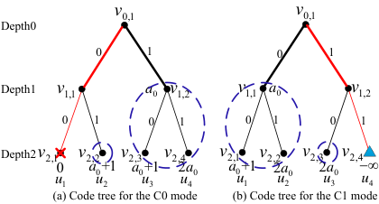
Generally, for the punctured source bits on the code tree, we have the following lemmas.

Now, we consider the performance analysis of polar or RCPP codes on the code tree. Because each path $\omega_{n}$ is relative to a polarized channel $i$ (refer to footnote 1), the corresponding upper bound of Bhattacharyya parameter $A_{n}\left(\omega_{n}\right)=\log_{2}\left(Z_{n}^{u}\left(\omega_{n}\right)\right)$ can be iteratively evaluated by using (5) or (8) in a log scale. This calculation includes two operators, that is, the adding-one operator $O_{a}:\mathbb{R}\to\mathbb{R},O_{a}(x)=x+1$ and the doubling operator $O_{d}:\mathbb{R}\to\mathbb{R},O_{d}(x)=2x$. Given the initial value of the root node $A_{0}=a_{0}$, a sequence of numbers $A_{1}(\omega_{1}),\cdots,A_{n}(\omega_{n})$ can be recursively calculated by

where $g_{l}\in\left\{O_{a},O_{d}\right\}$. From (8), when $b_{l}=0$, the operator $g_{l}=O_{a}$ is applied and when $b_{l}=1$, the operator $g_{l}=O_{d}$ is used.

Obviously, during the $n$ iterations of the $A_{n}(\omega_{n})$, we enumerate doubling $d_{H}(\omega_{n})$ times and adding-one $f_{H}(\omega_{n})$ times. And these two weights satisfy $d_{H}(\omega_{n})+f_{H}(\omega_{n})=n$.

We introduce two types of spectrum distances, SD1 and SD0, defined by the expectation of path weight and complemental weight respectively.

Hereafter, we use SD0/SD1/JSD as the main metrics to evaluate and optimize the puncturing table. If these metrics of one puncturing scheme are very close to those of the original polar code, this scheme will generate an optimal RCPP code.

Consider the single-bit puncturing under C0 mode. In this case, puncturing at different locations is equivalent regardless of a slight variation in its code tree.

The quasi-uniform puncturing (QUP) algorithm proposed in [15] can be outlined as follows.

1. Stage 1)

   Initialize the table $\mathscr{T}_{N}$ as all ones, and then set the first $Q$ bits as zeros;

2. Stage 2)

   Perform bit-reversal permutation on the table $\mathscr{T}_{N}$ and obtain the puncturing table.

The puncturing table generated by the QUP algorithm is constructive and regular, thereby providing useful tool for the practical application of coding and decoding.

This theorem is proved in [15].

Theoretically, the optimal puncturing table of RCPP codes can be optimized by a brute-force search of the distance spectra (for ML decoding) or BLER bounds (for SC decoding). However, the exhausted search for all the puncturing patterns is difficult to be realized. We are, therefore, concerned with the puncturing scheme to optimize the spectrum distances.

References

- [1] E. Arıkan, “Channel polarization: a method for constructing capacity achieving codes for symmetric binary-input memoryless channels,” IEEE Trans. Inf. Theory, vol. 55, no. 7, pp. 3051-3073, July 2009.
- [2] J. Hagenauer, “Rate-compatible punctured convolutional codes (RCPC Codes) and their applications,” IEEE Trans. Commun., vol. 36, no. 4, pp. 389-400, April 1988.
- [3] D. N. Rowitch and L. B. Milstein, “On the performance of hybrid FEC/ARQ system using rate compatible punctured turbo (RCPT) codes,” IEEE Trans. Commun., vol. 48, no. 6, pp. 948-959, June 2000.
- [4] E. Arıkan and E. Telatar, ”On the rate of channel polarization,” in Proc. IEEE Int. Symp. Inform. Theory (ISIT), pp. 1493-1495, July 2009.
- [5] N. Goela, S. B. Korada, and M. Gastpar, “On LP decoding of polar codes,” Proc. IEEE ITW, pp. 1-5, Sep. 2010.
- [6] I. Tal and A. Vardy, “List decoding of polar codes,” in Proc. IEEE Int. Symp. Inform. Theory (ISIT), pp. 1-5, 2011.
- [7] Y. Fan, C. Xia, J. Chen, C. Tsui, et al., “A Low-Latency List Successive-Cancellation Decoding Implementation for Polar Codes,” IEEE J. Sel. Areas Commun., vol. 34, no. 2, pp. 303-317, Feb. 2016.
- [8] K. Niu and K. Chen, “CRC-aided decoding of polar codes,” IEEE Commun. Lett., vol. 16, no. 10, pp. 1668-1671, Oct. 2012.
- [9] B. Li, H. Shen, and D. Tse, “An adaptive successive cancellation list decoder for polar codes with cyclic redundancy check,” IEEE Commun. Lett., Vol. 16, No. 12, pp. 2044-2047, 2012.
- [10] K. Niu and K. Chen, “Stack decoding of polar codes,” Electronics Letters, vol. 48, no. 12, pp. 695-697, 2012.
- [11] K. Chen, K. Niu and J. R. Lin, “Improved successive cancellation decoding of polar codes,” IEEE Trans. Commun., vol. 61, no. 8, pp. 3100-3107, 2013.
- [12] K. Niu, K. Chen, J. R. Lin, and Q. T. Zhang, “Polar codes: primary concepts and practical decoding algorithms,” IEEE Commun. Mag., pp. 192-203, July 2014.
- [13] A. Eslami and H. Pishro-Nik, “A practical approach to polar codes,” in Proc. IEEE Int. Symp. Inform. Theory (ISIT), pp. 16-20, 2011.
- [14] A. Eslami and H. Pishro-Nik, “On finite-length performance of polar codes: stopping sets, error floor, and concatenated design,” IEEE Trans. Commun., vol. 61, no. 3, March 2013.
- [15] K. Niu, K. Chen, and J. R. Lin, “Beyond turbo codes: rate-compatible punctured polar codes,” in Proc. IEEE International Conference on Communications, pp. 3423-3427, 2013.
- [16] D. M. Shin, S.-C. Lim, and K. Yang, “Design of length-compatible polar codes based on the reduction of polarizing matrices,” IEEE Trans. Commun., vol. 61, no. 7, pp. 2593-2599, 2013.
- [17] R. Wang and R. Liu, “A novel puncturing scheme for polar codes,” IEEE Commun. Lett., vol. 18, no. 12, pp. 2081-2084, 2014.
- [18] V. Miloslavskaya, “Shortened polar codes,”IEEE IEEE Trans. Inf. Theory, vol. 61, no. 9, pp. 4852-4865, 2015.
- [19] L. Zhang, Z. Y. Zhang, et. al., “On the puncturing patterns for punctured polar codes,” in Proc. IEEE Int. Symp. Inform. Theory (ISIT), pp. 121-125, 2014.
- [20] M. Valipour and S. Yousefi, “On probablistic weight distribution of polar codes,” IEEE Commun. Lett., vol. 17, no. 11, pp. 2120-2123, 2013.
- [21] Z. Z. Liu, K. Chen, K. Niu, and Z. Q. He, “Distance spectrum analysis of polar codes,” in Proc. IEEE Wireless Commun. Networking Conf. (WCNC) , pp. 490-495, April 2014.
- [22] P. Trifonov, “Efficient design and decoding of polar codes,” IEEE Trans. Commun., vol. 60, no. 11, pp. 3221-3227, Nov. 2012.
- [23] S. Lin and D. J. Costello Jr., Error Control Coding: Fundamentals and Applications (2nd ed.), Pearson Education, 2004.
- [24] K. F. Riley, M. P. Hobson, S. J. Bence, Mathematical methods for physics and engineering (3rd ed.), Cambridge University Press, p. 118, 2010.
- [25] 3GPP TS 36.212: “Multiplexing and channel coding,” Release 8, 2009.
- [26] Q. Zhang, A. Liu, X. Pan and K. Pan, “CRC Code Design for List Decoding of Polar Codes,” IEEE Commun. Lett., vol. 21, no. 6, pp. 1229-1232, Jun. 2017.
- [27] 3GPP TSG R1-1610137: “LDPC Rate Compatible Design Overview,” Qualcomm Incorporated, Lisbon, Portugal, Oct. 2016.