Unequal-Time Correlators for Cosmology
Abstract
Measurements of the power spectrum from large-scale structure surveys have to date assumed an equal-time approximation, where the full cross-correlation power spectrum of the matter density field evaluated at different times (or distances) has been approximated either by the power spectrum at a fixed time, or in an improved fashion, by a geometric mean . In this paper we investigate the expected impact of the geometric mean ansatz, and present an application in assessing the impact on weak gravitational lensing cosmological parameter inference, using a perturbative unequal-time correlator. As one might expect, we find that the impact of this assumption is greatest at large separations in redshift where the change in the amplitude of the matter power spectrum can be as much as percent for Mpc-1. However, of more concern is that the corrections for small separations, where the clustering is not close to zero, may not be negligibly small. In particular, we find that for a Euclid- or LSST-like weak lensing experiment the assumption of equal-time correlators may result in biased predictions of the cosmic shear power spectrum, and that the impact is strongly dependent on the amplitude of the intrinsic alignment signal. To compute unequal-time correlations to sufficient accuracy will require advances in either perturbation theory to high -modes, or extensive use of simulations.
Keywords:
Suggested keywordspacs
Valid PACS appear hereI Introduction
We consider evolving scalar fields in cosmology. We define an evolving three-dimensional random field , where labels a local three dimensional coordinate defined at a time ; equivalently labels a coordinate distance and we may use these interchangeably. For such an evolving three-dimensional random field we can choose a time coordinate and define a local plane wave Fourier transform as
| (1) |
where is a three dimensional wavenumber, and we use the notation of [1]. Even this equation involves a subtlety; we observe on the past light cone, so measurements are made not at a single time slice. In writing this, we assume that we evolve the fields to a common time slice, and we assume in this paper that the integration volume is small enough that the evolution is small enough that it can be done essentially perfectly. This then ensures that universal homogeneity is preserved in these local fields labelled with .
This field considered could be, for instance, the density fluctuation , or the Newtonian potential defined at time . For any two fields each with a time label, the cross-correlation power spectrum, which is assumed to be isotropic, is defined by
| (2) |
and we have exploited the homogeneity discussed above. From here we will use the notation for clarity. The projection of a field on the sky is defined using projection kernels such that
| (3) |
where is a surface that labels the projection and characterises the time when the projection is performed, and represents direction on the sky. A simple example of is a Gaussian centred on with a certain width. Expanding in terms of spherical harmonics, the angular cross-power spectrum of two different projections, is defined as
| (4) | |||||
where are spherical Bessel functions of order and are spherical harmonics. Here we consider the case that two fields and are different projections of the same underlying field and hence probe the same underlying power spectrum but via different projection kernels and respectively. This is easily generalised to different fields, in which case the cross-power spectrum is involved.
In the full expression of equation (4) the power spectrum is that between two different, unequal, times. We refer to as the unequal-time correlator. In cosmology however underlying power spectra are usually only expressed as a function of and a single time, i.e., , encoding the Fourier correlations at a given comoving distance, but not correctly describing the correlations between comoving distances.
To overcome this issue a mixed equal-time approximation was introduced in cosmology [2], where the geometric mean of the two equal-time power spectra has been assumed: . This approximation is justified by assuming that the correlation of the underlying (matter overdensity) field is restricted to small-scales in cosmology, and that over such scales the look-back time is approximately equal () therefore either or could be used instead of . The geometric mean approximation is then used as an algebraic convenience such that the integrals in equation (4) can be separated. A further justification is given that the Bessel function integrals may reduce to a delta-function for for large . These assumptions are tested in this paper.
II Unequal-time power spectra
To compute the power spectrum we need to refer to the correlation between the underlying fields in equation (2). In the cosmological context the underlying field of interest is often the matter overdensity ; where is the matter density at a position and comoving time , and is the mean matter density. This can be expanded [3, 4] perturbatively in terms of a growth factor , that is independent of scale, and a transfer function
| (5) |
where is the three-dimensional Fourier transform of . involves products and integrals of terms of – which is the density field that can be computed from linear gravitational theory [3]. For such terms become complicated and numerically challenging to compute.
We can now take correlations of equation (5) in both the unequal-time and the equal-time cases. For the unequal-time correlation we have
| (6) | |||||
where are the power spectra corresponding to the perturbatively expanded at order , see e.g. [4]. is the linear growth factor at comoving time to the power. In the fourth line we expand this expression to include all terms up to .
The geometric mean equal-time ansatz is that . By squaring equation (6) and multiplying equation (7) as required the differences between the two cases become clear
| (8) | |||||
and
| (9) | |||||
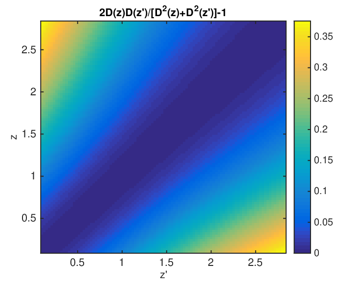
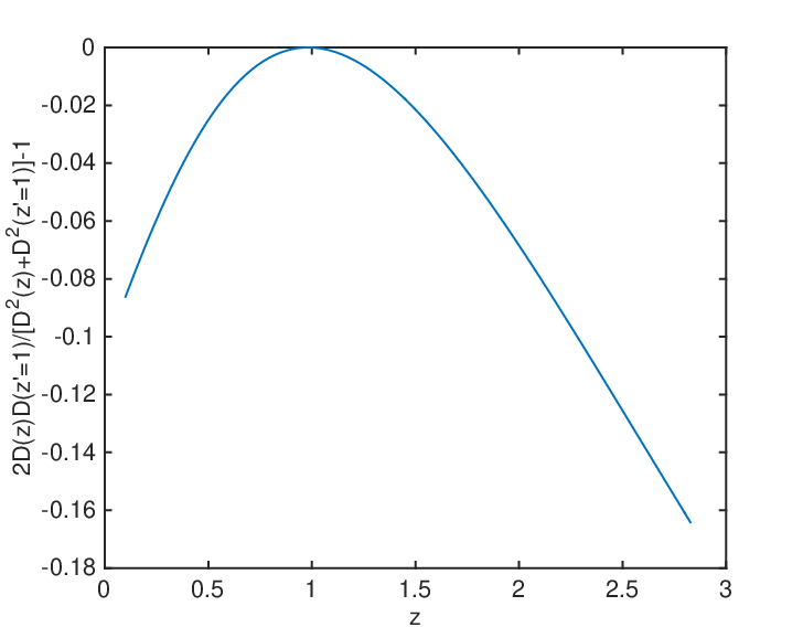
where each term can be compared. We see that many terms are in common, but a few coincide only if , which evidently only holds when . From here we will label comoving time with redshift , where the assumption of a cosmology is implicit. In Figure 1 we show the magnitude of this approximation as a function of redshift for a concordance cosmology.
 |
 |
 |
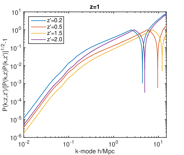 |
In Figure 2 we show and calculated using equations (6) and (7)11 1 For these calculations we use Cosmolopy http://roban.github.io/CosmoloPy/docAPI/cosmolopy.perturbation-module.html to compute the growth factor, and the order perturbation code for , , and available from E. Komatsu here http://wwwmpa.mpa-garching.mpg.de/~komatsu/CRL/powerspectrum/density3pt/pkd/.. We see that the impact of the equal-time approximation is largest at large redshift separations and increases in amplitude at small-scales where the and become dominant. For separations in redshift the change in the amplitude of the matter power spectrum can be as much as for Mpc-1. However, it is not clear yet whether the large deviations at large are important, since the correlation of the fields is likely to be very small here. We will return to this later.
An alternative formulation of an unequal-time correlation is to use an ‘eikonal’ phase [6, 7, 8, 9, 10] where the matter overdensity perturbations can be written like [9]
| (10) |
where represent fluctuations on short scales, and are linear-scale perturbations; this equation assumes a growing mode only. The unequal-time power spectrum is then expressed as the equal-time version multiplied by exponential damping term that depends on the separation in time; see for example [9] section 2.2. In this case unequal-time correlations are due to the mixing of long wavelength (or ‘soft’) modes with shorter wavelength modes. It is found that for equal times these have no impact on the amplitude of the power spectrum, which is consistent with the conclusion we find in this Section, but that for unequal-times there can be significant changes [7]. In [11] it is shown how to link the eikonal phase representation to a perturbation approach similar to that used here. [9, 10] derive power spectrum and bispectrum consistency conditions for the equal and unequal-time cases using this formalism.
II.1 Bessel/Lommel Effects
Despite the amplitude of the underlying power spectrum being different in the unequal-time and equal-time cases the integration over two Bessel functions in equation (4) may be expected to down-weight the impact of such an effect for a projected field. Indeed when integrating over multiple Bessel functions an orthogonality relation holds
| (11) |
where are the arguments corresponding to zeros of the spherical Bessel functions[12, 13]. However for the general case, where non-zero parts of the spherical Bessel function are integrated over, this orthogonality relation does not hold. There have been several investigations into the regimes where this expression is applicable for cosmology [14, 15]. In the case that there are such integrals over such a relation can be applied in the derivation of quantities for cosmology. However in the case of projected fields, that we investigate here, this is not appropriate because the equivalent expression that appears in equation (4) involves an integral over -mode. In the constant power spectrum case, and an upper -mode limit of , we would have expressions like
| (12) |
which is only applicable for a discretely sampled field in comoving distance such that are zeros of the spherical Bessel functions, this is clearly not the case. In [2, 16, 17] the case of is discussed which results in
| (13) |
but this is not a practical case for cosmology, and furthermore the full expression for does not converge to limit as we will discuss.
To investigate the effect of the Bessel integrations we explore the functions
| (14) |
for the unequal-time and equal-time cases respectively. These enter in equation (4), and similarly for the equal-time case, and are then integrated over with the projection kernels to generate the projected power spectra,
| (15) |
Equations (14) are also equal to the projected power spectra when the projection kernels are delta-functions e.g. . We assume the same as in Section II, where the integration is over range Mpc-122 2 We use the Matlab integration routine quadgk with a relative tolerance of and an absolute tolerance of , that are sufficient for numerical convergence, see e.g. Figure 4.. In Figure 3 we show the functions for several different -modes and redshift values.
 |
 |
It can be seen that the functional form of is sharply peaked about but has a non-zero tail out to large separations . Again we find large differences between the unequal-time and equal-time cases, with up to a factor 100 difference for large separations in redshift. The highly oscillatory nature of the functions is a real effect – not noise in the calculation (estimated error bars from the numerical integration are smaller than the linewidth in Figure 3). This highly oscillatory nature is a result of multiple Bessel functions in the solution moving in and out of phase as the values of change. For the case of a constant power spectrum (that is not a function of -mode) the equations (14) have an analytic solution given by Lommel’s integrals [12, 13] which are also rederived in [14]
| (16) |
where are Bessel functions of the first kind. We note that Lommels integrals do not converge to a delta-function as (equation 13), but become undefined. In Figure 4 we compare the numerical calculations used in this paper with the analytic solution in equations (16) and find that the difference at least a factor of ten smaller than the amplitude of .
 |
 |
II.2 Projection Effects
The final part of equation (4) that we consider is the effect of the projection kernels . In Figure 3 and equation (14) we have already investigated the case that . A further case that has been investigated in [1] is the case that , when the ‘Limber approximation’ can be applied to equation (4); this is applied in the equal-time case when the limits on the -mode integral are , and a Laplace transform can be used. We note that in the unequal-time case the derivation of [1] is not applicable because the and integrations are not separable.
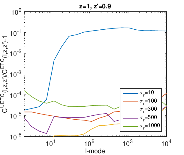
To investigate the effect of the projection kernels we consider to be at a fixed redshift: and use a Gaussian projection kernel for . We choose to be the comoving distance at . We then vary the width of the Gaussian projection kernel . In Figure 5 we show the fractional change in the projected power spectra for two different corresponding to redshifts of and . Again the non-smooth nature of these plots is a real feature of the oscillatory nature of the unequal-time computations.
 |
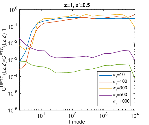 |
As expected projected cross-correlation power spectra with large redshift separations are affected more by the equal-time approximation, which can also be seen in Figures 1 and 3. Narrow, well-separated kernels are affected most. Broader kernels integrate over a range of redshifts, including separations where the effect is smaller, and reducing the overall impact. We also find that high -modes are modified more than small -modes, which is consistent with the underlying power spectrum being affected most at high (Figure 2). For widely-separated bins in redshift the change in the projected power spectrum can be over over scales . Therefore the cases in cosmology where the equal-time approximation is expected to have greatest impact are those where widely-separated tomographic redshift bins are used, with narrow projection kernels.
III Application
As shown in the previous section the difference between equal-time-approximated projected power spectra and the full unequal-time case is expected to become important for cross-correlations between widely separated redshift bins of fields that have a sharply-peaked projection kernels. An example of such a fields in cosmology are the cross-correlations between tomographic redshift bins of the weak lensing intrinsic alignment effect.
Weak lensing is an integrated effect, whereby the image of a distant galaxy is distorted by the gravitational lensing effect caused by matter perturbations along a line of sight; and is therefore by nature a projected field. In weak lensing the observed ellipticity is (to first order) a sum of the intrinsic (unlensed) ellipticity; the additional ellipticity caused by the gravitational lensing effect, , known as shear; and any noise effect: . When taking the covariance of these quantities and constructing projected fields (as in equation 4) the result is a sum of four terms:
| (17) |
where refers to the shear-shear correlations, to the cross-correlation between the intrinsic ellipticity and shear, and to intrinsic-intrinsic correlations. The correlation is expected to be zero (or at least very small) but we include it here for completeness.
The weak lensing observable is proportional to derivatives of the Newtonian potential therefore the inner integration over -mode in equation (4) is over the power spectrum of the Newtonian potential ,
| (18) |
for the case, where the inner power spectrum is related to the matter power spectrum through Poisson’s equations, which introduces a factor of so that (up to a cosmology-dependent multiplicative constant)
| (19) |
and similarly for the equal-time case, which can be compared to equations (14) and (15). We include a factor of here, being the result of angular derivatives relating the weak lensing observable (shear) to the projected Newtonian potential (see [2, 18]).
The unlensed observed ellipticity of a galaxy can be affected by the local gravitational potential, therefore the projection kernel in equation (4) is proportional to a delta function in this case. The shear effect is integrated along the line of sight and the projection kernel is a combination of angular diameter distances that determine the geometric gravitational lensing effect. We follow the notation of [19, 18] and define the power spectra using equation (4) where the two fields are combinations of and , with projection kernels given by
| (20) |
where is the comoving distance probability distribution for galaxies in a bin labelled with . The shear kernel is given by
| (21) |
where is the current Hubble parameter, is the current dimensionless matter density, is the speed of light in vacuum, is the dimensionless scale factor, for and zero otherwise; here we assume a flat geometry. The functions are and ; where is the linear growth factor, is the mean matter density at redshift , Mpc3, and is a free parameter that has a fiducial value of . This model for the intrinsic alignment power spectrum is the ‘linear alignment model’ discussed in [20] (see [21] for a recent review).
We use a fiducial Euclid-like33 3 http://euclid-ec.org weak lensing survey [22] (this is also similar to an LSST survey [23]), with a survey area of square degrees, a surface number density of galaxies of per square arcminute, a number density distribution given by , and a Gaussian photometric redshift distribution with standard deviation ; the function is given by the convolution of the in each tomographic redshift bin and the photometric redshift distribution. We use tomographic redshift bins with central redshifts given by . We compute these power spectra for the unequal-time and equal-time cases where the underlying power spectra are given in equations (6) and (7) where for the equal-time case we use the ansatz .

In Figure 6 we show the difference between the projected power spectra computed in the unequal-time and equal-time cases
| (22) |
We find that the term is most affected since its amplitude is relatively large and it requires a narrow kernel. The term has a combination of two narrow kernels but its amplitude is smaller relative to the total power spectrum. The term is also affected but at a typically lower amplitude than the term. If narrower redshift bins were used then the amplitude of the difference should increase. The change in power spectrum is certainly small, but in fact the requirements on are particularly stringent for weak lensing surveys. We can assess the impact of these changes by computing the integrated effect over the differences
| (23) |
complementary formulations are provide for this quantity in [24, 25, 26], the sum is over all redshift bin pairs and is the total number of redshift bin pairs. In general a non-zero will change the amplitude of the power spectrum and bias cosmological parameter inference. As discussed in [25] the requirement on the amplitude of this quantity is for a Euclid- or LSST-like weak lensing survey to return unbiased results on the dark energy equation of state parameters, this requirement is an allowance for all systematic effects including instrumental and algorithmic quantities. For our fiducial set we find that , which would account for of the requirement44 4 Using the more conservative definition for equation (23) in [24], that includes a normalisation we find that , which would account for of the requirement..
Because the equal time ansatz is expected to affect projected power spectra with narrow kernels in redshift, and the intrinsic alignment power spectrum is such a power spectrum, we investigate the impact of changing the amplitude of intrinsic alignment signal. In Figure 7 we change the parameter , that has a fiducial value of and show how the integrated change in the power spectrum, varies. In the left axes we show this normalised by the required value of , and the right axes shows the unnormalised value. The current range in this parameter is approximately [27]. We find as expected that the the impact of the equal time assumption becomes more prominent as the amplitude of the intrinsic alignment signal increases.

These results serve as an example of the type of impact that the assumption of equal-time correlators may have in cosmology, however the current precision of the perturbative approach to representing the matter power spectrum over a large range of -modes, and the lack of good predictions for how the unequal-time power spectrum behaves as a function of cosmological parameters, mean that the precise numerical results are only indicative of the full impact which requires further investigation.
IV Conclusion
In this paper we have presented a full projected field formalism for cosmology that includes the integration over an unequal-time correlator of the matter overdensity power spectrum . This relaxes an assumption that has been made in cosmology to date where individual or mixed equal-time correlators of the matter overdensity have been used, either and ansatz [2], or alternatively simply or .
We investigated the impact of the assumption of equal-time correlators by expanding both and perturbatively. We find that the impact of this assumption is largest at large separations in redshift where the change in the amplitude of the matter power spectrum can be as much as for Mpc-1. For projected fields we find that the impact is dependent on the width of the projection kernel. For Gaussian kernels with full-width-half-maxima of Mpc we find a effect for large redshift separations . Therefore observed power spectra that have narrow projections kernels and cross-correlations between widely-separated redshift bins are expected to be affected by the equal-time approximation.
One application where there are narrow projected kernels and widely separated redshift bins is the computation of weak lensing two-point correlation functions and power spectra – where in particular the contribution from intrinsic alignments (unlensed ellipticities) has local projection kernels in comoving coordinates. We find that for a Euclid- or LSST-like weak lensing experiment the assumption of equal-time correlators could introduce biases in the measurements of cosmological parameters, and that this is strongly dependent on the amplitude of the intrinsic alignment signal. However, due to the lack of good models for how cosmological parameters affect unequal-time correlators, these results are indicative only and require further investigation.
Unequal-time correlators have been investigated previously in [28, 29, 30, 31] in the study of cosmic strings. To determine unequal-time correlations analytically is an involved calculation, and in particular for the matter overdensity field perturbation theory at high -mode would make a full analytic solution challenging. In this paper we compute the matter power spectrum using perturbation theory to third order and use -modes with Mpc-1. One approach to include unequal-time correlators in cosmological statistics will be to extend this approach for arbitrary cosmological parameters and to high precision; such work that has begun in studies for equal-time correlators e.g. [32, 33]. As noted by [7] the eikonal phase representation of matter overdensity perturbations results in equal-time correlations being unaffected but unequal-time correlations being damped – this is a consistent with the results we find here where the equal-time case would require a lower matter power spectrum amplitude to fit the same data. Another approach will be to determine the unequal-time power spectra directly from simulations of the matter field such as [34, 35].
When designing statistics in cosmology great care must be taken to investigate the impact of any assumption or approximation used. We find that the equal-time approximation can potentially have a large impact on cosmological parameter inference. Unequal-time correlators can be computed using either perturbation to high -modes or from simulations, both of which require attention in order for future cosmological results to be unbiased.
Acknowledgements.
TDK is supported by a Royal Society University Research Fellowship. We thank E. Komatsu for making his perturbatively computed power spectrum code public.References
- [1] M. Loverde and N. Afshordi, Phys. Rev. D 78, 123506 (2008), eprint 0809.5112.
- [2] P. G. Castro, A. F. Heavens, and T. D. Kitching, Phys. Rev. D 72, 023516 (2005), eprint astro-ph/0503479.
- [3] A. F. Heavens, S. Matarrese, and L. Verde, MNRAS 301, 797 (1998), eprint astro-ph/9808016.
- [4] D. Jeong and E. Komatsu, ApJ 651, 619 (2006), eprint astro-ph/0604075.
- [5] Planck Collaboration, P. A. R. Ade, N. Aghanim, M. Arnaud, M. Ashdown, J. Aumont, C. Baccigalupi, A. J. Banday, R. B. Barreiro, J. G. Bartlett, et al., AAP 594, A13 (2016), eprint 1502.01589.
- [6] B. Jain and E. Bertschinger, ApJ 456, 43 (1996), eprint astro-ph/9503025.
- [7] F. Bernardeau, N. van de Rijt, and F. Vernizzi, Phys. Rev. D 85, 063509 (2012), eprint 1109.3400.
- [8] F. Bernardeau, N. Van de Rijt, and F. Vernizzi, Phys. Rev. D 87, 043530 (2013), eprint 1209.3662.
- [9] I. Ben-Dayan, T. Konstandin, R. A. Porto, and L. Sagunski, JCAP 2, 026 (2015), eprint 1411.3225.
- [10] M. Garny, T. Konstandin, R. A. Porto, and L. Sagunski, JCAP 11, 032 (2015), eprint 1508.06306.
- [11] P. Creminelli, J. Gleyzes, M. Simonović, and F. Vernizzi, JCAP 2, 051 (2014), eprint 1311.0290.
- [12] G. Watson, A Treatise on the Theory of Bessel Functions, Cambridge Mathematical Library (Cambridge University Press, 1995), ISBN 9780521483919, URL https://books.google.co.uk/books?id=Mlk3FrNoEVoC.
- [13] M. Abramowitz and I. Stegun, Handbook of Mathematical Functions: With Formulas, Graphs, and Mathematical Tables, Applied mathematics series (Dover Publications, 1964), ISBN 9780486612720, URL https://books.google.co.uk/books?id=MtU8uP7XMvoC.
- [14] K. B. Fisher, O. Lahav, Y. Hoffman, D. Lynden-Bell, and S. Zaroubi, MNRAS 272, 885 (1995), eprint astro-ph/9406009.
- [15] A. F. Heavens and A. N. Taylor, MNRAS 275, 483 (1995), eprint astro-ph/9409027.
- [16] N. Baddour, J. Opt. Soc. Am. A 27, 2144 (2010), URL http://josaa.osa.org/abstract.cfm?URI=josaa-27-10-2144.
- [17] B. Leistedt, A. Rassat, A. Réfrégier, and J.-L. Starck, AAP 540, A60 (2012), eprint 1111.3591.
- [18] T. D. Kitching, J. Alsing, A. F. Heavens, R. Jimenez, J. D. McEwen, and L. Verde, ArXiv e-prints (2016a), eprint 1611.04954.
- [19] T. D. Kitching, A. F. Heavens, and S. Das, MNRAS 449, 2205 (2015), eprint 1408.7052.
- [20] C. M. Hirata and U. Seljak, Phys. Rev. D 70, 063526 (2004), eprint astro-ph/0406275.
- [21] B. Joachimi, M. Cacciato, T. D. Kitching, A. Leonard, R. Mandelbaum, B. M. Schäfer, C. Sifón, H. Hoekstra, A. Kiessling, D. Kirk, et al., SSR 193, 1 (2015), eprint 1504.05456.
- [22] R. Laureijs, J. Amiaux, S. Arduini, J. . Auguères, J. Brinchmann, R. Cole, M. Cropper, C. Dabin, L. Duvet, A. Ealet, et al., ArXiv e-prints (2011), eprint 1110.3193.
- [23] LSST Science Collaboration, P. A. Abell, J. Allison, S. F. Anderson, J. R. Andrew, J. R. P. Angel, L. Armus, D. Arnett, S. J. Asztalos, T. S. Axelrod, et al., ArXiv e-prints (2009), eprint 0912.0201.
- [24] R. Massey, H. Hoekstra, T. Kitching, J. Rhodes, M. Cropper, J. Amiaux, D. Harvey, Y. Mellier, M. Meneghetti, L. Miller, et al., MNRAS 429, 661 (2013), eprint 1210.7690.
- [25] M. Cropper, H. Hoekstra, T. Kitching, R. Massey, J. Amiaux, L. Miller, Y. Mellier, J. Rhodes, B. Rowe, S. Pires, et al., MNRAS 431, 3103 (2013), eprint 1210.7691.
- [26] A. Amara and A. Réfrégier, MNRAS 391, 228 (2008), eprint 0710.5171.
- [27] C. Heymans, E. Grocutt, A. Heavens, M. Kilbinger, T. D. Kitching, F. Simpson, J. Benjamin, T. Erben, H. Hildebrandt, H. Hoekstra, et al., MNRAS 432, 2433 (2013), eprint 1303.1808.
- [28] P. P. Avelino, E. P. S. Shellard, J. H. P. Wu, and B. Allen, Physical Review Letters 81, 2008 (1998), eprint astro-ph/9712008.
- [29] U.-L. Pen, U. Seljak, and N. Turok, Physical Review Letters 79, 1611 (1997), eprint astro-ph/9704165.
- [30] A. Albrecht, R. A. Battye, and J. Robinson, Physical Review Letters 79, 4736 (1997), eprint astro-ph/9707129.
- [31] A. Albrecht, R. A. Battye, and J. Robinson, Phys. Rev. D 59, 023508 (1999), eprint astro-ph/9711121.
- [32] G. Somogyi and R. E. Smith, Phys. Rev. D 81, 023524 (2010), eprint 0910.5220.
- [33] D. Blas, M. Garny, T. Konstandin, and J. Lesgourgues, JCAP 11, 039 (2014), eprint 1408.2995.
- [34] D. Nelson, A. Pillepich, S. Genel, M. Vogelsberger, V. Springel, P. Torrey, V. Rodriguez-Gomez, D. Sijacki, G. F. Snyder, B. Griffen, et al., Astronomy and Computing 13, 12 (2015), eprint 1504.00362.
- [35] J. Schaye, R. A. Crain, R. G. Bower, M. Furlong, M. Schaller, T. Theuns, C. Dalla Vecchia, C. S. Frenk, I. G. McCarthy, J. C. Helly, et al., MNRAS 446, 521 (2015), eprint 1407.7040.
- [36] A. N. Taylor and T. D. Kitching, MNRAS 408, 865 (2010), eprint 1003.1136.
- [37] W. Hu, ApJL 522, L21 (1999), eprint astro-ph/9904153.
- [38] T. D. Kitching, A. N. Taylor, M. Cropper, H. Hoekstra, R. K. E. Hood, R. Massey, and S. Niemi, MNRAS 455, 3319 (2016b), eprint 1507.05334.
- [39] B. Joachimi and S. L. Bridle, AAP 523, A1 (2010), eprint 0911.2454.
*