On a multivariate renewal-reward process involving time delays and discounting: Applications to IBNR process and infinite server queues

Many situations in which processes restart probabilistically at renewal instants and there are non-negative rewards associated with each renewal epoch, are well described by a multivariate renewal-reward process. For example, a multivariate reward function can be viewed as an accumulated cost from different types of properties or infrastructures caused by a single catastrophe event, which is of interest in actuarial science and reliability analysis. The asymptotic distribution and the asymptotic expansion for the covariance function of the rewards were studied by [24] and [1] who extended the result of [5] to multivariate case. In the context of actuarial science, much research about the aggregate discounted claims has been done on its moment under renewal claim arrival processes. For example, [15], [16], [17], and [18] analyzed the renewal process, and [34] looked at the dependent renewal process.

In this paper, we assume that there are time lags added to the original arrival times of renewal process. These delayed renewal epochs allow us to study the quantities related to infinite server queues with correlated batch arrivals and multivariate Incurred But Not Reported (IBNR) claims where there is a delay in reporting or payment for claims. Furthermore, rewards are accumulated at a discounted value. A direct application to some problems in infinite server queues includes the case, for example, when the bulk size random variable is multivariate (i.e. correlated) and the service time distribution is dependent on the type of input. In this case a multivariate reward function incorporating time delays up to time $t$ (with zero discounting factor) is essentially the number of customers in the system up to time $t$. In the infinite server queues with multiple batch Markovian arrival streams, a time-dependent matrix joint generating function of the number of customers in the system was derived by [22]. For the univariate case, IBNR claim count with batch arrivals was considered by [9] and the total discounted IBNR claim amount was studied by [14]. For the multivariate case, [33] provided expressions for the joint moments of multivariate IBNR claims which are recursively computable. For the number of IBNR claims, a direct relation to the number of customers in the infinite server queues with batch arrivals is well known as discussed in the literature, e.g. [12], [14], [29], [30], [31]. The transient behavior of a distribution of the number of customer in various multichannel bulk queues was studied in [6]. See also [4] for example.

Let us introduce the model more precisely. We shall suppose that the batch arrival process $\{N_{t}\}_{t\geq 0}$ is a renewal process with a sequence of independent and identically distributed (iid) positive continuous random variables (rv)s $(T_{i})_{i\in\mathbb{N}}$ representing the arrival time of the $i$th batch with $T_{0}\equiv 0$. Let $\tau_{i}=T_{i}-T_{i-1}$ be the interarrival time of the $i$th batch with a common probability density function (pdf) $f$, distribution $F$, and the Laplace transform ${\cal L}^{\tau}(u)=\mathbb{E}[e^{-u\tau_{1}}]$ for $u\geq 0$. Also we denote the renewal function and renewal density $t\mapsto m(t):=\mathbb{E}[N_{t}]$ and $u(t)=\frac{d}{dt}m(t)$ respectively. Each batch arrival contains several ($k$) types of inputs which may simultaneously occur from the same renewal event (e.g. [24], [33]). Let us denote the $j$-type of input from the $i$th batch as $X_{i,j}$ where $\{(X_{i,1},\ldots,X_{i,k})\}_{i\in\mathbb{N}}$ is a sequence of iid random vectors. A vector for generic multivariate input variables is denoted as $X=(X_{1},X_{2},\ldots,X_{k})$. Here multivariate input values are assumed to be dependent on the occurrence time and/or the adjusted time by adding a random delay. This time delay for the $j$-type of input from the $i$th batch is denoted by $L_{i,j}$ where $(L_{i,j})_{i\in\mathbb{N}}$ is a sequence of iid random variables with a common cumulative distribution function $W_{j}(t)=1-\overline{W}_{j}(t)$, and such that $(L_{i,j})_{i\in\mathbb{N},j=1,...,k}$ is a sequence of independent random variables. A generic time delay rv for the $j$-type of input is denoted by $L_{j}$. For the sake of simplicity let us assume a constant force of interest $\delta$ to discount input values to time 0, and define the following discounted compound delayed process

where

Here, we can interpret the process $\{Z(t)\}_{t\geq 0}$ in two different ways. The first one is related to actuarial science: we suppose that aggregate claim amounts (or claim severities) $X_{i,j}$ in the branch $j\in\{1,\ldots,k\}$ of an insurance company is caused by the event arriving at time $T_{i}$. Instead of being dealt with immediately, they are (within a batch) subject to a delay $L_{i,j}$ until being reported. $Z_{j}(t)$ then represents the discounted total claim amounts of such IBNR claims in the branch $j$. The second one is related to queueing theory: let us consider a single queue containing $k$ types of customers in an infinite-server queue model. Here customers arrive according to a renewal process $\{N_{t}\}_{t\geq 0}$ with corresponding arrival times $(T_{i})_{i\in\mathbb{N}}$. At each arrival instant $T_{i}$ a batch of correlated customers $(X_{i,1},\ldots,X_{i,k})$ enters the system, with $X_{i,j}\in\mathbb{N}$. For each customer of class $j\in\{1,\ldots,k\}$ (of which number is $X_{i,j}$) the service time $L_{i,j}$ is the same. The service times $(L_{i,j})_{i\in\mathbb{N},\ j=1,\ldots,k}$ are thus assumed to be independent, although $L_{i,1},\ldots,L_{i,k}$ possibly have different distributions, i.e. service times are different according to the type of customer class. For example, if $\delta=0$, the model is reduced to that of $G/G/\infty$ queues with multiple types of customer classes in a batch. As an illustration, let us look at the particular case where $(X_{1},\ldots,X_{k})$ follows a multinomial distribution with parameters $M\in\mathbb{N}^{*}$ and a probability vector $(p_{1},\ldots,p_{k})$ where $p_{j}\geq 0$ and $\sum_{j=1}^{k}p_{j}=1$. This models a situation where at every instant $T_{i}$ exactly $M$ customers arrive, each of which belongs to class $j$ with probability $p_{j}$. Then $X_{j}$ represents the number of customers of class $j$ in this batch. See Figure 1.

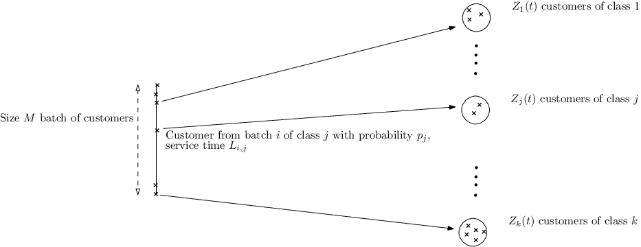
The simplest scenario is when $M=1$, where each customer arrives according to renewal process $\{N_{t}\}_{t\geq 0}$, and belongs to class $j$ with probability $p_{j}$. Because of these two alternative interpretations in actuarial science and queueing theory as explained above, we will refer the $L_{i,j}$’s as either "delay" or "service" times, without ambiguity.

We note that it is usually difficult to derive a distribution for this discounted compound delayed process $Z(t)$ since there is no concrete representation for an inversion of the complicated moment generating function (mgf) for this quantity in a general arrival process $\{N_{t}\}_{t\geq 0}$. In this sense, it is appealing to study the long-term behavior of the process in terms of its moment and distribution. From [33], explicit expressions for the joint moments of $Z(t)=(Z_{1}(t),...,Z_{k}(t))$ are recursively obtainable. However, an analytic expression of the lower moment which appears in its integral term, is required for the calculation of the higher moment. Also, it is necessary to know an explicit form of the renewal density $u(t)$ for the evaluation of this moment. Therefore, our objective here is to develop simpler approximation methods such as asymptotics and bound results for the joint moments of $Z(t)$. To the best of our knowledge, these kinds of approximation approaches have never been developed in the analysis of a multivariate renewal-reward process with discounted inputs and time delays. Also, a relationship between multivariate discounted IBNR claim process and quantities studied in infinite server queues with correlated batch arrivals and a discounting factor is firstly exploited in this paper. Moreover, we shall also consider the case with exponential time delays in a general arrival process and provide asymptotic results for the joint moments. In this case, for light tailed interclaim time and single input, we are able to quantify the approximation precision by providing many terms for the asymptotics for the first order moment of our process. We note that this approach was previously found in [5, Lemma 1] where a 2-term asymptotic expression for a general renewal reward process without delays was provided, see also [24] and [1] for an expansion of the covariance. In particular, some asymptotic results regarding queueing theoretic applications such as the workload in the $G/M/\infty$ system, are obtained.

In most cases in this paper, we suppose that the discounted factor $\delta$ is real and non negative because of its discounting role. However it has to be pointed out that, mathematically speaking, Definitions (1) and (2) can in some cases be extended to some complex $\delta$, as will be the case in Section 5 where $\delta\in\mathbb{C}$ is needed for technical purposes. It will also be convenient to define the process $\tilde{Z}(t)=\tilde{Z}(t,\delta)=(\tilde{Z}_{1}(t),\ldots,\tilde{Z}_{k}(t))=e^{\delta t}Z(t)$, i.e.

Although $\tilde{Z}(t)$ does not have a direct actuarial or queueing interpretation, it will turn out that most results will concern this process rather than $Z(t)$.

It is convenient to introduce the function $t\mapsto\varphi_{\ell,n}(t)$ for $\ell<n$,

where

Following [33], we define $\tilde{b}_{n}(t)$ by

Throughout the paper, ${\cal E}(\mu)$ denotes an exponential distribution with a mean $1/\mu$. We denote $|A|$ as the cardinal of $A$ for any finite set $A$.

We assume that a vector $X$ admits joint moments of all order. We recall that a rv $Y\geq 0$ has New Better than Used (NBU) distribution if its survival function satisfies $\mathbb{P}(Y>x+y)\leq\mathbb{P}(Y>x)\mathbb{P}(Y>y)$ for all non negative $x$ and $y$. Lastly, we denote assumptions (A1), (A1’) and (A2) by:

It is noted that (A2) is substantive in several queueing and actuarial applications. One way of viewing the upper bounded condition in queueing theory is to consider the number of arriving customers being fixed or limited (as illustrated in the example in Figure 1). When the claim severity distribution follows a general family of NBU classes, some interesting applications in relation to reinsurance premium calculation are discussed in [13, Section 3.1].

An important consequence of (A1) is the following result, of which proof is given at the beginning of Section 7.

The aim of this section is to briefly review the results obtained in [33] that will be the starting point of most of the results in the present paper, and to recover some particular results when claims arrive according to a Poisson process. Following notation in [33, Section 3.3], we let for all $t\geq 0$ and $s=(s_{1},\ldots,s_{k})\in\mathbb{R}^{k}$,

From [33, Section 3.3], we know that the mgf of $Z(t)$ in (5) satisfies

and from (36) of [33], (4) is recursively obtained as

and in particular, when $n=n(i)$, it reduces to

Also, from [33, Theorem 3], $\tilde{M}_{n}(t)$ defined in (6) satisfies

where $\overline{\omega}_{\delta,i}(t)$ and $\tilde{b}_{n}(t)$ are respectively given by (9) and (10). It is standard that the solution to (15) is given by $\tilde{M}_{n}(t)=\int_{0}^{t}\tilde{b}_{n}(t-y)dm(y)$ for all $t\geq 0$, which is equivalent to (13) and (14), up to multiplication by $e^{\eta_{n}\delta t}$. However, as pointed out in [33], this solution is hardly explicit in practice because $\tilde{b}_{n}(.)$ depends on $\tilde{M}_{\ell}(.)$, $\ell<n$. Only when $n=n(i)$, we find a simple expression which was also considered in [33, Example 3] as $k=1$ and $n_{1}=1$. In this case, one finds (10) given by

So, in general, the expression for $\tilde{M}_{n}(t)$ at time $t$ depends on the whole trajectory of $\tilde{M}_{\ell}(y)$, $\ell<n$, for $y\in[0,t]$ as it is also obvious from (13). Furthermore, the renewal function $t\mapsto m(t)$ is not always explicit.

The above corollary is useful to find a closed form expression for $\tilde{\psi}(s,t)$ when arrivals occur according to a Poisson process.

Two remarks are to be deduced from Proposition 4. First, since the pdf of the exponential distribution is upper bounded, Condition (A1) is fulfilled, and thus one has from upcoming Theorem 10 in Section 3, that $\tilde{Z}(t)$ converges in distribution towards some light tailed random vector ${\cal Z}_{\infty}$. Thus, it is immediate from (18) that the mgf of ${\cal Z}_{\infty}$ is, when $\tau_{1}\sim{\cal E}(\lambda)$, given by

Second, one is able to recover some well known result in the $M/G/\infty$ queue by setting $\delta=0$. For example, when $k=1$ and $X=X_{1}$, one computes that $M^{*}_{t,X}(s)=1+(e^{s}-1)\overline{W}(t)$, and (18) reduces to

recovering that the distribution of the number of customers in an infinite server queue with Poisson arrivals of intensity $\lambda$ is Poisson distributed with parameter $\lambda\int_{0}^{t}\overline{W}(v)dv$ at time $t$, see [27, Theorem 1, p.160]. When $\delta=0$, (18) in Proposition 4 is similar to the results obtained in Section 3.1 of [19], concerning infinite server queues with Poisson arrivals.

We are interested in the limiting behaviour of the process $\tilde{Z}(t)$ when arrivals and delays have a general distribution. It may be difficult to compute its distribution in all generality, however some information may be obtained if we add a specific assumption on the arrival process $\{N_{t}\}_{t\geq 0}$. Our first immediate result is convergence of joint moments of $\tilde{Z}(t)$:

A direct consequence of Proposition 5 when $n=n(i)$ with (16) yields the result for the first moment in the following corollary.

We note that in Proposition 5 coefficients $\chi_{n}$, $n\in\mathbb{N}^{k}$ are in general not directly available, as the function $t\mapsto\tilde{b}_{n}(t)$ in the integral (19) does not have an easy expression, and are defined recursively in the function of $t\mapsto\tilde{M}_{\ell}(t)$, $\ell<n$. We thus provide in the following easily computable bounds for the $\chi_{n}$’s and a uniform upper bound in $t$ for $\tilde{M}_{n}(t)$ if we impose that (A1) holds.

We remark that (23) provides a simple bound for the limiting joint moments which is immediately computable, and (24) gives some information on the transient joint moments (i.e. on the whole trajectory $t\mapsto\tilde{M}_{n}(t)$). It is often more complicated to compute (24), as $C$ is not always explicit (as explained in Remark 2). Also, the existence of the upper bound $C$ is proved thanks to the fact that $\lim_{t\to\infty}u(t)=1/\mathbb{E}(\tau_{1})$, as shown in the proof of Lemma 1 at the beginning of Section 7, which implies that $1/\mathbb{E}(\tau_{1})\leq C$. Hence (23) is tighter than (24).

In the following example, we calculate higher moments of two types of discounted IBNR claims until time $t$ under the same model setting as [33, Section 4] for comparison purposes.

Proposition 8 is useful for two reasons. First, as illustrated in the previous example, we remark that coefficients $R_{n}$, $n\in\mathbb{N}^{k}$, in (25) can be easily computed because $R_{n}$ is a linear function of the $R_{\ell}$, $\ell<n$, and only involves the joint moments of $X=(X_{1},\ldots,X_{k})$, the Laplace transform of the $L_{1}$,…,$L_{k}$ as well as their expectations. So, simple bounds are available, which is useful since it is not possible in general to compute the distribution (or even moments) of the process. Second, Proposition 5 leads to $\tilde{M}_{n}(t)$ converging towards $\chi_{n}$. Since $\tilde{M}_{n}(t)$ is the joint moments of $\mathbb{R}^{k}$ valued process $\{\tilde{Z}(t)\}_{t\geq 0}$, this suggests in turn that this process converges in distribution. As convergence of moments does not always implies convergence in distribution, we give some sufficient conditions such that this latter holds, and we prove it thanks to the bounds obtained in Proposition 8. In the following we address the limiting behaviour in distribution of process $\{\tilde{Z}(t)\}_{t\geq 0}$ under (A1) and (A2).

Let us note that Theorem 10 holds for general interarrival times $\tau_{i}$ that satisfy (A1), and general time delays $L_{j}$’s. The aim of this subsection is to prove that the $\chi_{n}$’s are explicit when the $L_{j}$’s are exponentially distributed. We suppose for simplicity that all $L_{j}$’s for $j=1,\ldots,k$, have the same distribution ${\cal E}(\mu)$, for some $\mu>0$. Note that we may obtain similar results as will be given in the following for more general cases such as a mixture or a combination of exponential distributions, but the expressions would only be more complicated.

For notational convenience, let ${\cal L}^{M}_{n}(u)$ and ${\cal L}^{b}_{n}(u)$ for $u\geq 0$ and $n\in\mathbb{N}^{k}$, be the Laplace transforms of $\tilde{M}_{n}(\cdot)$ and $\tilde{b}_{n}(\cdot)$ respectively

Note that these Laplace transforms exist (i.e. the integrals converge) respectively when $u>0$ and $u\geq 0$ since $\tilde{M}_{n}(y)$ converges to some finite limit $\chi_{n}$ as $y\to\infty$, and $\tilde{b}_{n}(\cdot)$ is integrable (as proved in Proposition 5). The following lemma gives a recursive expression of ${\cal L}^{b}_{n}(u)$.

References

- [1] Aliyev, R. and Bayramov, V. On the asymptotic behaviour of the covariance function of the rewards of a multivariate renewal-reward process. Statistics and Probability Letters, 127: 138–149, 2017.
- [2] Asmussen, S. Applied probability and queues. Springer, 2000.
- [3] Brown, M. and Ross, S.M. Renewal Reward Processes. Issue 93 of Technical report, Cornell University, Department of Operations Research, 1969.
- [4] Brown, M. and Ross, S.M. Some results for infinite server Poisson queues. Journal of Applied Probability, 6: 604–611, 1969.
- [5] Brown, M. and Solomon, H. A second-order approximation for the variance of a renewal reward process. Stochastic Processes and their Applications, 3(3): 301–314, 1975.
- [6] Chaudhry, M. L. and Templeton, J.G.C. A first course in bulk queues. New York: Wiley, 1983.
- [7] Dombry, C. and Rabehasaina, L. High order expansions for renewal functions and applications to ruin theory. Annals of Applied Probability, 27(4): 2342–2382, 2017.
- [8] Feller, W. An introduction to probability theory and its applications VII. John Wiley & Sons, 1968.
- [9] Guo, L., Landriault, D. and Willmot, G.E. On the analysis of a class of loss models incorporating time dependence. European Actuarial Journal, 3: 273–294, 2013.
- [10] Haviland, E. K. On the momentum problem for distribution functions in more than one dimension. American Journal of Mathematics, 57(3): 562–568, 1935.
- [11] Izawa, T. The bivariate gamma distribution. In: Climate and Statistics (in Japanese), 4: 9–15, 1953.
- [12] Karlsson, J.E. A stochastic model for the lag in reporting of claims. Journal of Applied Probability, 11: 382–387, 1974.
- [13] Kayid, M. A general family of NBU classes of life distributions. Statistical Methodology, 4: 185–195, 2007.
- [14] Landriault, D., Willmot, G.E. and Xu, D. Analysis of IBNR claims in renewal insurance models. Scandinavian Actuarial Journal, 2017(7): 628–650, 2017.
- [15] Léveillé, G. and Adékambi, F. Covariance of discounted compound renewal sums with a stochastic interest rate. Scandinavian Actuarial Journal, 2: 138–153, 2011.
- [16] Léveillé, G. and Garrido, J. Moments of compound renewal sums with discounted claims. Insurance: Mathematics and Economics, 28(2): 217–231, 2001.
- [17] Léveillé, G. and Garrido, J. Recursive moments of compound renewal sums with discounted claims. Scandinavian Actuarial Journal, 2: 98–110, 2001.
- [18] Léveillé, G., Garrido, J. and Wang, Y.F. Moment generating functions of compound renewal sums with discounted claims. Scandinavian Actuarial Journal, 3: 165–184, 2010.
- [19] Liu, L., Kashyap, B.R.K. and Templeton J.G.C. On the system. Journal of Applied Probability, (27)3: 671–683, 1990.
- [20] Losidis, S. and Politis, K. A two-sided bound for the renewal function when the interarrival distribution is IMRL. Statistics and Probability Letters, 125: 164–170, 2017.
- [21] Marshall, A.W. and Olkin I. Life Distributions, Structure of nonparametric, semiparametric and parametric families. Springer, 2007.
- [22] Masuyama, H. and Takine, T. Analysis of an infinite-server queue with batch Markovian arrival streams. Queueing Systems, 42: 269–296, 2002.
- [23] Neuts, M.F. and Chen S.Z. The infinite server queue with semi-Markovian arrivals and negative exponential services. Journal of Applied Probability, (9)1: 178–184, 1972.
- [24] Patch, B. Nazarathy, Y. and Taimre, T. A correction term for the covariance of renewal-reward processes with multivariate rewards. Statistics and Probability Letters, 102: 1–7, 2015.
- [25] Smith, W.L. Renewal theory and its ramifications. Journal of the Royal Statistical Society, Series B, 20: 243–302, 1958.
- [26] Smith, W. The infinitely many server queue with semi-markovian arrivals and customer-dependent exponential service times. Operations Research, (20)4: 907–912, 1972.
- [27] Takács, L. Introduction to the theory of queues. Oxford University press, 1962.
- [28] Willmot, G.E. A queueing theoretic approach to the analysis of the claims payment process. Transaction of Society of Actuaries, 42: 447–497, 1990.
- [29] Willmot, G.E. and Drekic, S. On the transient analysis of the queue. Operations Research Letters, 28: 137–142, 2001.
- [30] Willmot, G.E. and Drekic, S. Transient analysis of some infinite server queues. Recent Advances in Statistical Methods, 1: 329–338, 2002.
- [31] Willmot, G.E. and Drekic, S. Time-dependent analysis of some infinite server queues with bulk Poisson arrivals. INFOR, 47: 297–303, 2009.
- [32] Willmot, G.E. and Woo, J.-K. Surplus Analysis of Sparre Andersen Insurance Risk Processes. Springer Actuarial, 2017.
- [33] Woo, J.-K. On multivariate discounted compound renewal sums with time-dependent claims in the presence of reporting/payment delays. Insurance: Mathematics and Economics, 70: 354–363, 2016.
- [34] Woo, J.-K. and Cheung, E.C.K. A note on discounted compound renewal sums under dependency. Insurance: Mathematics and Economics, 52(2): 170–179, 2013.