Alternating maps on Hatcher-Thurston graphs

Jesús Hernández Hernández

Abstract

Let $S_{1}$ and $S_{2}$ be connected orientable surfaces of genus $g_{1},g_{2}\geq 3$ , $n_{1},n_{2}\geq 0$ punctures, and empty boundary. Let also $\varphi:\mathcal{HT}(S_{1})\rightarrow\mathcal{HT}(S_{2})$ be an edge-preserving alternating map between their Hatcher-Thurston graphs. We prove that $g_{1}\leq g_{2}$ and that there is also a multicurve of cardinality $g_{2}-g_{1}$ contained in every element of the image. We also prove that if $n_{1}=0$ and $g_{1}=g_{2}$ , then the map $\widetilde{\varphi}$ obtained by filling the punctures of $S_{2}$ , is induced by a homeomorphism of $S_{1}$ .

Introduction

Suppose $S_{g,n}$ is an orientable surface of finite topological type, with genus $g\geq 3$ , empty boundary, and $n\geq 0$ punctures. The (extended) mapping class group is the group of isotopy classes of self-homeomorphisms of $S_{g,n}$ .
In 1980 (see [4]), Hatcher and Thurston introduce the Hatcher-Thurston complex of a surface, which is the $2$ -dimensional CW-complex whose vertices are multicurves called cut systems, $1$ -cells are defined as elementary moves between cut systems, and $2$ -cells are defined as appropriate “triangles”, “squares” and “pentagons”. See Section 1 for the details. They used this complex to prove that the index 2 subgroup of $\mathrm{Mod}^{*}(S_{g,n})$ of orientation preserving isotopy classes, is finitely presented. The $1$ -skeleton of this complex is called the Hatcher-Thurston graph, which we denote by $\mathcal{HT}(S_{g,n})$ .
There is a natural action of $\mathrm{Mod}^{*}(S_{g,n})$ on the Hatcher-Thurston complex by automorphisms, and in [9] Irmak and Korkmaz proved that the automorphism group of the Hatcher-Thurston complex is isomorphic to $\mathrm{Mod}^{*}(S_{g,n})$ . Inspired by the different results in combinatorial rigidity on other simplicial graphs (like the curve graph in [11] and [7], and the pants graph in [1]), we obtain analogous results concerning simplicial maps between Hatcher-Thurston graphs.
Let $S_{1}=S_{g_{1},n_{1}}$ and $S_{2}=S_{g_{2},n_{2}}$ with $g_{1},g_{2}\geq 2$ and $n_{1},n_{2}\geq 0$ . A simplicial map $\varphi:\mathcal{HT}(S_{1})\rightarrow\mathcal{HT}(S_{2})$ is alternating if the restriction to the star of any vertex, maps cut systems that differ in exactly $2$ curves to cut systems that differ in exactly $2$ curves. See Section 1 for the details. In Section 2 we prove our first result concerning this type of map:

Theorem A.

1.

$g_{1}\leq g_{2}$ .
2.

There exists a unique multicurve $M$ in $S_{2}$ with $g_{2}-g_{1}$ elements such that $M\subset\phi(C)$ for all cut systems $C$ in $S_{1}$ .

A consequence of this theorem is that whenever we have an edge-preserving alternating map $\phi:\mathcal{HT}(S_{1})\rightarrow\mathcal{HT}(S_{2})$ (where the conditions of Theorem A are satisfied), we can then induce an edge-preserving alternating map $\varphi:\mathcal{HT}(S_{1})\rightarrow\mathcal{HT}(S_{2}\backslash M)$ where $M$ is the multicurve obtained by Theorem A, and $S_{2}\backslash M$ is connected (due to the nature of Theorem A) and has genus $g_{1}$ . This means we can focus solely on the case where $g_{1}=g_{2}$ . However, due to the nature of $\mathcal{HT}(S_{1})$ and the techniques available right now, it is quite difficult to study these maps if $n_{1}>0$ , and it is possible to have edge-preserving alternating maps if $n_{1}<n_{2}$ that are obviously not induced by homeomorphisms, e.g. creating $n_{2}-n_{1}$ punctures in $S_{1}$ .
A way around this particular complication is wondering if this is the only way for the edge-preserving alternating maps to be not induced by homeomorphisms, leading to the following question:

Question B.

Let $S_{1}$ , $S_{2}$ and $S_{3}$ be connected orientable surfaces, with genus $g\geq 3$ , $n_{1},n_{2}\geq 0$ punctures for $S_{1}$ and $S_{2}$ respectively, and assume $S_{3}$ is closed. Let $\phi:\mathcal{HT}(S_{1})\rightarrow\mathcal{HT}(S_{2})$ be an edge-preserving alternating map. Is there a way to induce a well-defined map $\varphi:\mathcal{HT}(S_{3})\rightarrow\mathcal{HT}(S_{3})$ from $\phi$ by filling the punctures of $S_{1}$ and $S_{2}$ ? If so, is $\varphi$ induced by a homeomorphism?

In Section 3 we answer this question for a particular case. If $\pi_{\mathcal{HT}}$ is the map induced by filling the punctures of $S_{2}$ , we have the following result:

Theorem C.

Let $S_{1}$ and $S_{2}$ be connected orientable surfaces, with genus $g\geq 3$ and empty boundary, and assume $S_{1}$ is closed. Let $\phi:\mathcal{HT}(S_{1})\rightarrow\mathcal{HT}(S_{2})$ be an edge-preserving and alternating map. Then

\widetilde{\phi}\mathrel{\mathop{:}}=\pi_{\mathcal{HT}}\circ\phi:\mathcal{HT}(S_{1})\rightarrow\mathcal{HT}(S_{1})

is induced by a homeomorphism of $S_{1}$ .

This implies that the only way to obtain a map from $\mathcal{HT}(S_{1})$ to $\mathcal{HT}(S_{2})$ that is edge-preserving and alternating, is to use a homeomorphism of $S_{1}$ and then puncture the surface to obtain $S_{2}$ .
Theorem C is proved by using $\phi$ to induce maps between the underlying curves of the cut systems, and eventually induce an edge-preserving self-map of the curve graph of $S_{1}$ (see Section 3 for the details). Then, by the Theorem A of [7] (the second article of a series of which this work is also a part) we have that said self-map is induced by a homeomorphism.
Later on, in Section 4 we prove a consequence of Theorems A and C concerning isomorphisms and automorphisms between Hatcher-Thurston graphs.

Corollary D.

Let $S_{1}$ and $S_{2}$ be connected orientable surfaces, with genus $g_{1},g_{2}\geq 2$ respectively, with empty boundary and $n_{1},n_{2}\geq 0$ punctures respectively. If $\phi:\mathcal{HT}(S_{1})\rightarrow\mathcal{HT}(S_{2})$ is an isomorphism, we have that $\phi$ is an alternating map and $g_{1}=g_{2}$ . Moreover, this implies that if $S=S_{g,0}$ with $g\geq 3$ , then $\mathrm{Aut}(\mathcal{HT}(S))$ is isomorphic to $\mathrm{Mod}^{*}(S)$ .

We must remark that this work is the published version of the fourth chapter of the author’s Ph.D. thesis (see [5]), and the results here presented are dependent on the results found in [7], which is the published version of the third chapter. There we prove that for any edge-preserving map between the curve graphs of a priori different surfaces (with certain conditions on the complexity and genus for the surfaces) to exist, it is necessary that the surfaces be homeomorphic and that the edge-preserving map be induced by a homeomorphism between the surfaces.
Acknowledgements: The author thanks his Ph.D. advisors, Javier Aramayona and Hamish Short, for their very helpful suggestions, talks, corrections, and specially for their patience while giving shape to this work.

1 Preliminaries and properties

In this section we give several definitions and prove several properties of the Hatcher-Thurston graph. Here we suppose $S=S_{g,n}$ with genus $g\geq 1$ and $n\geq 0$ punctures.
A curve $\alpha$ is a topological embedding of the unit circle into the surface. We often abuse notation and call “curve” the embedding, its image on $S$ or its isotopy class. The context makes clear which use we mean.
A curve is essential if it is neither null-homotopic nor homotopic to the boundary curve of a neighbourhood of a puncture.
The (geometric) intersection number of two (isotopy classes of) curves $\alpha$ and $\beta$ is defined as follows:

i(\alpha,\beta)\mathrel{\mathop{:}}=\min\{|a\cap b|:a\in\alpha,b\in\beta\}.

Let $\alpha$ and $\beta$ be two curves on $S$ . Here we use the convention that $\alpha$ and $\beta$ are disjoint if $i(\alpha,\beta)=0$ and $\alpha\neq\beta$ .
A multicurve $M$ is either a single curve or a set of pairwise disjoint curves. A cut system $C$ of $S$ is a multicurve of cardinality $g$ such that $S\backslash C$ is connected.
Similarly, a curve $\alpha$ is separating if $S\backslash\{\alpha\}$ is disconnected, and is nonseparating otherwise. Note that a cut system can only contain nonseparating curves, and also $S\backslash C$ has genus zero, thus a cut system $C$ can be characterized as a maximal multicurve such that $S\backslash C$ is connected.
Two cut systems $C_{1}$ and $C_{2}$ are related by an elementary move if they have $g-1$ elements in common and the remaining two curves intersect once.
The Hatcher-Thurston graph $\mathcal{HT}(S)$ is the simplicial graph whose vertices correspond to cut systems of $S$ , and where two vertices span an edge if they are related by an elementary move. We will denote by $\mathcal{V}(\mathcal{HT}(S))$ the set of vertices of $\mathcal{HT}(S)$ .
If $M$ is a multicurve on $S$ , we will denote by $\mathcal{HT}_{M}(S)$ the (possibly empty) full subgraph of $\mathcal{HT}(S)$ spanned by all cut systems that contain $M$ .

Remark 1.1.

Let $M$ and $M^{\prime}$ be multicurves on $S$ such that neither $\mathcal{HT}_{M}(S)$ nor $\mathcal{HT}_{M^{\prime}}(S)$ are empty graphs. Then $\mathcal{HT}_{M}(S)\subset\mathcal{HT}_{M^{\prime}}(S)$ if and only if $M^{\prime}\subset M$ . Also, if $M$ is a multicurve such that $\mathcal{HT}_{M}(S)$ is nonempty, then $\mathcal{HT}_{M}(S)$ is naturally isomorphic to $\mathcal{HT}(S\backslash M)$ .

Recalling previous work on the Hatcher-Thurston complex we have the following lemma.

Lemma 1.2 ([12]).

Let $S$ be an orientable connected surface of genus $g\geq 1$ , with empty boundary and $n\geq 0$ punctures. Then $\mathcal{HT}(S)$ is connected.

Note that this lemma and Remark 1.1 imply that if $M$ is a multicurve on $S$ such that $S\backslash M$ is connected, then $\mathcal{HT}_{M}(S)$ is connected.

1.1 Properties of $\mathcal{HT}(S)$

Let $C$ be a cut system on $S$ , and denote by $\mathcalligra{lk}\hskip 3.41418pt(C)$ the full subgraph spanned by the set of cut systems on $S$ that are adjacent to $C$ in $\mathcal{HT}(S)$ (often called the link of $C$ in $\mathcal{HT}(S)$ ). Intuitively, we want to relate the elements of $\mathcalligra{lk}\hskip 3.41418pt(C)$ that are obtained by replacing the same curve of $C$ ; this is done defining the relation $\thicksim_{C}$ in $\mathcalligra{lk}\hskip 3.41418pt(C)$ by

C_{1}\thicksim_{C}C_{2}\Leftrightarrow C_{1}\cap C=C_{2}\cap C.

We can easily check $\thicksim_{C}$ is an equivalence relation, and two cut systems are related in $\mathcalligra{lk}\hskip 3.41418pt(C)$ if they are obtained by replacing the same curve of $C$ as was desired. The equivalence classes of this relation will be called colours.
This definition implies that in $\mathcalligra{lk}\hskip 3.41418pt(C)$ there are $g$ colours, each corresponding to a curve in $C$ that was substituted; thus, we use the elements of $C$ to index these colours.

Remark 1.3.

We should note that if $C_{1},C_{2}\in\mathcalligra{lk}\hskip 3.41418pt(C)$ are such that $C_{1}\nsim_{C}C_{2}$ , then $C_{1}$ and $C_{2}$ share exactly $g-2$ curves.

Refer to caption — Figure 1: The cut systems $\{\alpha_{1},\beta,\alpha_{3},\alpha_{4}\}$ and $\{\alpha_{1},\beta^{\prime},\alpha_{3},\alpha_{4}\}$ are in the same colour with respect to $\{\alpha_{1},\ldots,\alpha_{4}\}$ , while $\{\alpha_{1},\alpha_{2},\beta^{\prime\prime},\alpha_{4}\}$ is not.

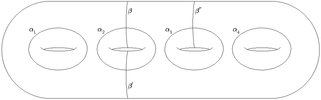
Let $\gamma$ be a nonseparating curve of $S$ . Following Irmak and Korkmaz’s work on the Hatcher-Thurston complex (for which we recall $\mathcal{HT}(S)$ is the $1$ -skeleton) in [9], we define the graph $X_{\gamma}^{S}$ as the simplicial graph whose vertices are the nonseparating curves $\beta$ on $S$ such that $i(\beta,\gamma)=1$ , and two vertices $\alpha$ and $\beta$ span an edge if $i(\alpha,\beta)=1$ .
In [9], we obtain the following result, modifying the statement to suit the notation used here.

Lemma 1.4 ([9]).

Let $S=S_{g,n}$ such that $g\geq 1$ and $n\geq 0$ , and $\gamma$ be a nonseparating curve on $S$ . Then $X_{\gamma}^{S}$ is connected.

A triangle on $\mathcal{HT}(S)$ is a set of three distinct cut systems on $S$ , whose elements pairwise span edges in $\mathcal{HT}(S)$ . Now we prove that for every triangle in $\mathcal{HT}(S)$ there exists a convenient multicurve contained in each cut system.

Lemma 1.5.

Let $S=S_{g,n}$ such that $g\geq 1$ and $n\geq 0$ punctures, and $T$ be a triangle on $\mathcal{HT}(S)$ . Then, there exists a unique multicurve $M$ , of cardinality $g-1$ , such that $M$ is contained in every element of $T$ .

Proof.

Let us denote $T=\{A,B,C\}$ . Since $A,B\in\mathcalligra{lk}\hskip 3.41418pt(C)$ then if $A\nsim_{C}B$ , by Remark 1.3, $|A\cap B|=g-2$ ; but then $A$ and $B$ would not be able to span an edge, contradicting $T$ being a triangle. Thus $A\thicksim_{C}B$ . Since $A\neq B$ we have $M=A\cap C=B\cap C$ is the desired multicurve of cardinality $g-1$ . ∎

Lemma 1.6.

Let $A,B,C$ be distinct cut systems on $S$ , such that $A,B\in\mathcalligra{lk}\hskip 3.41418pt(C)$ . Then $A\thicksim_{C}B$ if and only if there exists a finite collection of triangles $T_{1},\ldots,T_{m}$ such that $A,C\in T_{1}$ , $B,C\in T_{m}$ , and $T_{i}$ and $T_{i+1}$ share exactly one edge for $i=1,\ldots,m-1$ .

Proof.

If $g=1$ , then we obtain the desired result directly from Lemma 1.4, making $C=\{\gamma\}$ . So, suppose $g>1$ .
If $A\thicksim_{C}B$ , let $M=A\cap C=B\cap C$ be the multicurve of Lemma 1.5 with cardinality $g-1$ . Let $\alpha$ be the curve in $A\backslash M$ , $\beta$ be the curve in $B\backslash M$ and $\gamma$ be the curve in $C\backslash M$ . Since $A,B\in\mathcalligra{lk}\hskip 3.41418pt(C)$ then $\alpha$ and $\gamma$ intersect once, just the same as $\beta$ and $\gamma$ ; moreover, $\alpha$ , $\beta$ and $\gamma$ are nonseparating curves of $S\backslash M$ since $A$ , $B$ and $C$ are cut systems. Thus $\alpha$ and $\beta$ are vertices in $X_{\gamma}^{S\backslash M}$ , and by Lemma 1.4 there exists a finite collection of nonseparating (in $S\backslash M$ ) curves $c_{0},\ldots,c_{m}$ with $\alpha=c_{0}$ , $\beta=c_{m}$ and $c_{i}$ adjacent to $c_{i+1}$ in $X_{\gamma}^{S\backslash M}$ . Since every $c_{i}$ is a nonseparating curve of $S\backslash M$ , then $\{c_{i}\}\cup M$ is a cut system of $S$ for each $i$ ; in particular $A=\{c_{0}\}\cup M$ and $B=\{c_{m}\}\cup M$ . By construction, $T_{i+1}\mathrel{\mathop{:}}=\{\{c_{i}\}\cup M,C,\{c_{i+1}\}\cup M\}$ is a triangle for $i=0,\ldots,m-1$ , $T_{i}$ and $T_{i+1}$ share exactly one edge for $i=0,\ldots,m-1$ , $A,C\in T_{1}$ , and $C,B\in T_{m}$ .
Conversely, if $T_{1},\ldots,T_{m}$ is a finite collection of triangles such that $A,C\in T_{1}$ , $B,C\in T_{m}$ and $T_{i}$ and $T_{i+1}$ share exactly one edge for $i=1,\ldots,m-1$ , we denote by $M_{i}$ the multicurve corresponding to the triangle $T_{i}$ obtained by Lemma 1.5, in particular $A\cap C=M_{1}$ and $B\cap C=M_{m}$ . Let $D_{i}$ and $D_{i}^{\prime}$ be the cut systems in the triangle that span the edge shared by $T_{i}$ and $T_{i+1}$ ; since $D_{i}\cap D_{i}^{\prime}=M_{i}$ in $T_{i}$ and $D_{i}\cap D_{i}^{\prime}=M_{i+1}$ in $T_{i+1}$ , we have that $M_{i}=M_{i+1}$ for $i=1,\ldots,m-1$ . Thus $M_{i}=M_{j}$ for $i\neq j$ , so $A\cap C=B\cap C$ which by definition implies that $A\thicksim_{C}B$ . ∎

2 Proof of Theorem A

In this section, let all surfaces be of genus at least $2$ , possibly with punctures.
An alternating square in $\mathcal{HT}(S)$ is a closed path with four distinct consecutive vertices $C_{1}$ , $C_{2}$ , $C_{3}$ , $C_{4}$ such that $C_{1}\nsim_{C_{2}}C_{3}$ and $C_{2}\nsim_{C_{3}}C_{4}$ . So, $C_{1}$ and $C_{3}$ have exactly $g-2$ curves in common, and $C_{2}$ and $C_{4}$ have also exactly $g-2$ curves in common. In Figure 1 the cut systems $\{\alpha_{1},\alpha_{2},\alpha_{3},\alpha_{4}\}$ , $\{\alpha_{1},\beta,\alpha_{3},\alpha_{4}\}$ , $\{\alpha_{1},\beta,\beta^{\prime\prime},\alpha_{4}\}$ and $\{\alpha_{1},\alpha_{2},\beta^{\prime\prime},\alpha_{2}\}$ form an alternating square.

Lemma 2.1.

Let $C_{1}$ , $C_{2}$ , $C_{3}$ , $C_{4}$ be consecutive vertices of an alternating square in $\mathcal{HT}(S)$ . Then $C_{1}\cap C_{2}\cap C_{3}\cap C_{4}$ has cardinality $g-2$ .

Proof.

Since $C_{1},C_{3}\in\mathcalligra{lk}\hskip 3.41418pt(C_{2})$ , $C_{1}\cap C_{3}=C_{1}\cap C_{2}\cap C_{3}$ ; analogously $C_{1}\cap C_{3}=C_{1}\cap C_{4}\cap C_{3}$ . This implies that $C_{1}\cap C_{2}\cap C_{3}\subset C_{4}$ , thus $C_{1}\cap C_{2}\cap C_{3}\cap C_{4}=C_{1}\cap C_{3}$ . Given that $C_{1}\nsim_{C_{2}}C_{3}$ , we have $|C_{1}\cap C_{2}\cap C_{3}\cap C_{4}|=g-2$ . ∎

Lemma 2.2.

Let $C_{1},C_{2},C_{3}$ be cut systems on $S$ , such that $C_{1},C_{3}\in\mathcalligra{lk}\hskip 3.41418pt(C_{2})$ and $C_{1}\nsim_{C_{2}}C_{3}$ . There exists $C_{3}^{\prime}\in\mathcalligra{lk}\hskip 3.41418pt(C_{2})$ with $C_{3}^{\prime}\thicksim_{C_{2}}C_{3}$ , such that $C_{1}$ , $C_{2}$ , $C_{3}^{\prime}$ are consecutive vertices of an alternating square.

Proof.

Since $C_{1}\nsim_{C_{2}}C_{3}$ , let $M$ be the common multicurve of $C_{1}$ , $C_{2}$ and $C_{3}$ obtained by Lemma 1.5. Let also $\alpha,\beta,\alpha^{\prime},\beta^{\prime}$ be the curves such that $C_{1}=M\cup\{\alpha^{\prime},\beta\}$ , $C_{2}=M\cup\{\alpha,\beta\}$ and $C_{3}=M\cup\{\alpha,\beta^{\prime}\}$ .
Let $T$ be a regular neighbourhood of $\{\alpha,\alpha^{\prime}\}$ . Since $i(\alpha,\alpha^{\prime})=1$ , $T$ is homeomorphic to $S_{1,1}$ . Let $\beta^{\prime\prime}$ be a nonseparating curve of $S\backslash M$ such that $i(\beta,\beta^{\prime\prime})=1$ , and $\beta^{\prime\prime}$ is contained in $S\backslash T$ (that is possible since $S\backslash M$ has genus $2$ ). By construction we have the following: $C_{3}^{\prime}=M\cup\{\alpha,\beta^{\prime\prime}\}$ and $C_{4}=M\cup\{\alpha^{\prime},\beta^{\prime\prime}\}$ are cut systems such that $C_{3}^{\prime}\in\mathcalligra{lk}\hskip 3.41418pt(C_{2})\cap\mathcalligra{lk}\hskip 3.41418pt(C_{4})$ , $C_{4}\in\mathcalligra{lk}\hskip 3.41418pt(C_{1})\cap\mathcalligra{lk}\hskip 3.41418pt(C_{3})$ , $C_{3}\thicksim_{C_{2}}C_{3}^{\prime}$ , $C_{1}\nsim_{C_{2}}C_{3}^{\prime}$ and $C_{2}\nsim_{C_{3}^{\prime}}C_{4}$ . Thus $C_{1}$ , $C_{2}$ , $C_{3}^{\prime}$ , $C_{4}$ are the consecutive vertices of an alternating square. ∎

Let $S_{1}=S_{g_{1},n_{1}}$ and $S_{2}=S_{g_{2},n_{2}}$ with genus $g_{1}\geq 2$ , $g_{2}\geq 1$ and $n_{1},n_{2}\geq 0$ .
A simplicial map $\phi:\mathcal{HT}(S_{1})\rightarrow\mathcal{HT}(S_{2})$ is said to be edge-preserving if whenever $C_{1}$ and $C_{2}$ are two distinct cut systems that span an edge in $\mathcal{HT}(S_{1})$ , their images under $\phi$ are distinct and span an edge in $\mathcal{HT}(S_{2})$ .

Remark 2.3.

Note that if $\phi:\mathcal{HT}(S_{1})\rightarrow\mathcal{HT}(S_{2})$ is an edge-preserving map, then triangles are mapped to triangles.

The map $\phi$ is said to be alternating if for all cut systems $C$ on $S_{1}$ and all $C_{1},C_{2}\in\mathcalligra{lk}\hskip 3.41418pt(C)$ such that $C_{1}$ and $C_{2}$ differ by exactly two curves, then $\phi(C_{1})$ and $\phi(C_{2})$ differ by exactly two curves. Note that this condition says nothing about $\phi(C)$ and its relation with $\phi(C_{1})$ and $\phi(C_{2})$ .

Lemma 2.4.

Let $\phi:\mathcal{HT}(S_{1})\rightarrow\mathcal{HT}(S_{2})$ be an edge-preserving map, and $C_{1}$ , $C_{2}$ and $C_{3}$ be cut systems on $S_{1}$ with $C_{1},C_{3}\in\mathcalligra{lk}\hskip 3.41418pt(C_{2})$ . If $C_{1}\thicksim_{C_{2}}C_{3}$ , then $\phi(C_{1})\thicksim_{\phi(C_{2})}\phi(C_{3})$ . If $\phi$ is also alternating, then $C_{1}\nsim_{C_{2}}C_{3}$ implies $\phi(C_{1})\nsim_{\phi(C_{2})}\phi(C_{3})$ ; in particular alternating squares go to alternating squares.

Proof.

If $C_{1}\thicksim_{C_{2}}C_{3}$ , then by Lemma 1.6 there exists a finite collection of triangles $T_{1},\ldots,T_{m}$ with $C_{1},C_{2}\in T_{1}$ , $C_{2},C_{3}\in T_{m}$ , and $T_{i},T_{i+1}$ share one edge. By Remark 2.3 $\phi(T_{i})$ is a triangle for all $i=1,\ldots,m$ , with $\phi(C_{1}),\phi(C_{2})\in\phi(T_{1})$ , $\phi(C_{2}),\phi(C_{3})\in\phi(T_{m})$ and $\phi(T_{i}),\phi(T_{i+1})$ sharing one edge; thus, once again by Lemma 1.6, $\phi(C_{1})\thicksim_{\phi(C_{2})}\phi(C_{3})$ .
Let $\phi$ be also alternating, and $C_{1}\nsim_{C_{2}}C_{3}$ . By Remark 1.3 $C_{1},C_{3}$ differ by exactly $2$ curves and since $\phi$ is an edge-preserving alternating map, we have that $\phi(C_{1}),\phi(C_{3})\in N(\phi(C_{2}))$ and $\phi(C_{1}),\phi(C_{3})$ differ by exactly $2$ curves; so, $\phi(C_{1})\nsim_{\phi(C_{2})}\phi(C_{3})$ .
Let $\phi$ be an edge-preserving alternating map, and $\mathcal{S}$ be an alternating square with consecutive vertices $C_{1},\ldots,C_{4}$ . Since $C_{1},C_{3}\in\mathcalligra{lk}\hskip 3.41418pt(C_{2})\cap\mathcalligra{lk}\hskip 3.41418pt(C_{4})$ then $\phi(C_{1}),\phi(C_{3})\in N(\phi(C_{2}))\cap N(\phi(C_{4}))$ , and as proved above $\phi(C_{1})\nsim_{\phi(C_{2})}\phi(C_{3})$ and $\phi(C_{2})\nsim_{\phi(C_{3})}\phi(C_{4})$ (since $C_{1}\nsim_{C_{2}}C_{3}$ and $C_{2}\nsim_{C_{3}}C_{4}$ ). Therefore $\phi(\mathcal{S})$ is an alternating square. ∎

Note that this lemma allows us to see the importance of the alternating requirement for $\phi$ . If $\phi$ were only edge-preserving (or locally injective), we would not have enough information to be certain that alternating squares are mapped to alternating squares, which is an important requirement if we ever want $\phi$ to be induced by a homeomorphism. Moreover, the rest of the results presented here would be much more complicated to prove if at all possible.
Now we are ready to prove Theorem A (which is quite similar to a result about locally injective maps for the Pants complex, that appears as Theorem C in [1], though we must note that for some of the arguments in the proof being an alternating map is a key requirement).

Proof of Theorem A.

Let $A$ be a vertex of $\mathcal{HT}(S_{1})$ . Then let $\{B_{1},\ldots,B_{g_{1}}\}\subset\mathcalligra{lk}\hskip 3.41418pt(A)$ be a set of representatives for the colours of $\mathcalligra{lk}\hskip 3.41418pt(A)$ . Since $B_{i}\thicksim_{A}B_{j}$ if and only if $i=j$ then $\phi(B_{i})\thicksim_{\phi(A)}\phi(B_{j})$ if and only if $i=j$ , by Lemma 2.4; thus $\mathcalligra{lk}\hskip 3.41418pt(\phi(A))$ has at least a many colours as $\mathcalligra{lk}\hskip 3.41418pt(A)$ , so $g_{1}\leq g_{2}$ .
This implies that $M=\phi(B_{1})\cap\cdots\cap\phi(B_{g_{1}})$ has cardinality $g_{2}-g_{1}$ . We must also note that $M\subset\phi(A)$ . We can easily check that if $B\thicksim_{A}B_{i}$ for some $i$ , then $M\subset\phi(B)$ : by Lemma 2.4 $\phi(B)\thicksim_{\phi(A)}\phi(B_{i})$ , which means they were obtained from $\phi(A)$ by replacing the same curve, so $\phi(A)\cap\phi(B_{i})\subset\phi(B)$ ; since $M\subset\phi(A)\cap\phi(B_{i})$ , then $M\subset\phi(B)$ .
With this we have proved that for all $B\in A\cup\mathcalligra{lk}\hskip 3.41418pt(A)$ , $M\subset\phi(B)$ . Given that $\mathcal{HT}(S_{1})$ is connected, we only need to prove that given any element $B\in\mathcalligra{lk}\hskip 3.41418pt(A)$ , for all $C\in\mathcalligra{lk}\hskip 3.41418pt(B)$ , we have $M\subset\phi(C)$ . Let $B$ and $C$ be such cut systems.
If $C\thicksim_{B}A$ , then by Lemma 2.4 $\phi(C)\thicksim_{\phi(B)}\phi(A)$ , which means $\phi(C)$ and $\phi(A)$ were obtained by replacing the same curve of $\phi(B)$ , so $\phi(C)\cap\phi(B)=\phi(A)\cap\phi(B)$ . Since we have already proved that $M\subset\phi(B)$ and $M\subset\phi(A)$ then $M\subset\phi(A)\cap\phi(B)=\phi(C)\cap\phi(B)$ . Thus $M\subset\phi(C)$ .
If $C\nsim_{B}A$ , then by Lemma 2.2 there exists $C^{\prime}\in\mathcalligra{lk}\hskip 3.41418pt(B)$ with $C\thicksim_{B}C^{\prime}$ and $C^{\prime}\nsim_{B}A$ , such that $A,B,C^{\prime}$ are consecutive vertices of an alternating square $\Sigma$ . By Lemma 2.4 $\phi(\Sigma)$ is also an alternating square. Let $D$ the vertex of $\Sigma$ different from $A$ , $B$ and $C^{\prime}$ ; since $D\in\mathcalligra{lk}\hskip 3.41418pt(A)$ , we have proved above that $M\subset\phi(D)$ , thus $M\subset\phi(A)\cap\phi(B)\cap\phi(D)$ and as we have seen in the proof of Lemma 2.1, $\phi(A)\cap\phi(B)\cap\phi(C^{\prime})\cap\phi(D)=\phi(A)\cap\phi(B)\cap\phi(D)$ , so $M\subset\phi(C^{\prime})$ . Given that $C\thicksim_{B}C^{\prime}$ , this leaves us in the previous case, therefore $M\subset\phi(C)$ . ∎

3 Proof of Theorem C

Hereinafter, let $S_{1}=S_{g,0}$ and $S_{2}=S_{g,n}$ with $g\geq 3$ and $n\geq 0$ . Before giving the idea of the proof, we need the following definitions.
We define the complexity of $S_{g,n}$ , denoted by $\kappa(S_{g,n})$ as $3g-3+n$ . Note this is equal to the cardinality of a maximal multicurve.
If $S_{g,n}$ is such that $\kappa(S_{g,n})>1$ , the curve graph $\mathcal{C}(S_{g,n})$ , introduced by Harvey in [3], is the simplicial graph whose vertices correspond to the curves of $S$ , and two vertices span an edge if they are disjoint. We denote $\mathcal{V}(\mathcal{C}(S_{g,n}))$ the set of vertices of $\mathcal{C}(S_{g,n})$ .
If $S_{g,n}$ is such that $g\geq 1$ , the Schmutz graph $\mathcal{G}(S_{g,n})$ , introduced by Schmutz-Schaller in [10], is the simplicial graph whose vertices correspond to nonseparating curves of $S$ , and where two vertices span an edge if they intersect once. We denote by $\mathcal{V}(\mathcal{G}(S))$ the set of vertices of $\mathcal{G}(S)$ .
Idea of the proof: We proceed by using $\phi$ to induce a map $\psi:\mathcal{V}(\mathcal{G}(S_{1}))\rightarrow\mathcal{V}(\mathcal{G}(S_{2}))$ in such a way that $\phi(\{\alpha_{1},\ldots,\alpha_{g}\})=\{\psi(\alpha_{1}),\ldots,\psi(\alpha_{g})\}$ . Then we induce two maps $\widetilde{\phi}:\mathcal{HT}(S_{1})\rightarrow\mathcal{HT}(S_{1})$ and $\widetilde{\psi}:\mathcal{V}(\mathcal{G}(S_{1}))\rightarrow\mathcal{V}(\mathcal{G}(S_{1}))$ by filling the punctures of $S_{2}$ . These maps also verify that $\widetilde{\phi}(\{\alpha_{1},\ldots,\alpha_{g}\})=\{\widetilde{\psi}(\alpha_{1}),\ldots,\widetilde{\psi}(\alpha_{g})\}$ . Following the proofs of several properties of $\psi$ and $\widetilde{\psi}$ , we extend $\widetilde{\psi}$ to an edge-preserving map $\widehat{\psi}:\mathcal{C}(S_{1})\rightarrow\mathcal{C}(S_{1})$ which, by Theorem A in [7], is induced by a homeomorphism of $S_{1}$ . Therefore $\widetilde{\psi}$ is induced by a homeomorphism of $S_{1}$ .

3.1 Inducing $\psi:\mathcal{G}(S_{1})\rightarrow\mathcal{G}(S_{2})$ and $\widetilde{\psi}:\mathcal{G}(S_{1})\rightarrow\mathcal{G}(S_{1})$

Let $\alpha$ be a nonseparating curve. Recall that $\mathcal{HT}_{\{\alpha\}}(S_{1})$ is isomorphic to $\mathcal{HT}(S_{1}\backslash\{\alpha\})$ . Then, given an edge-preserving alternating map $\phi:\mathcal{HT}(S_{1})\rightarrow\mathcal{HT}(S_{2})$ we can obtain an edge-preserving alternating map $\phi_{\alpha}:\mathcal{HT}(S_{1}\backslash\{\alpha\})\rightarrow\mathcal{HT}(S_{2})$ . Applying Theorem A to $\phi_{\alpha}$ we know there exists a unique multicurve on $S_{2}$ of cardinality $1$ , contained in the image under $\phi$ of every cut system containing $\alpha$ ; we will denote the element of this multicurve as $\psi(\alpha)$ . In this way we have defined a function $\psi:\mathcal{V}(\mathcal{G}(S_{1}))\rightarrow\mathcal{V}(\mathcal{G}(S_{2}))$ .

Lemma 3.1.

Let $\phi:\mathcal{HT}(S_{1})\rightarrow\mathcal{HT}(S_{2})$ be an edge-preserving alternating map and $\psi:\mathcal{V}(\mathcal{G}(S_{1}))\rightarrow\mathcal{V}(\mathcal{G}(S_{2}))$ be the induced map on the nonseparating curves. If $\alpha$ and $\beta$ are nonseparating curves and $C$ a cut system on $S_{1}$ , then:

1.

If $\alpha\in C$ , then $\psi(\alpha)\in\phi(C)$ .
2.

If $\alpha\neq\beta$ and $\alpha,\beta\in C$ , then $\psi(\alpha)\neq\psi(\beta)$ .
3.

If $i(\alpha,\beta)=1$ , then $i(\psi(\alpha),\psi(\beta))=1$ .

Proof.

(1) Follows directly from the definition.
(2) Let $C=\{\alpha,\beta,\gamma_{1},\ldots,\gamma_{g-2}\}$ and let $C_{\alpha},C_{\beta},C_{\gamma_{1}},\ldots,C_{\gamma_{g-2}}$ be representatives of the colours in $\mathcalligra{lk}\hskip 3.41418pt(C)$ indexed by $\alpha,\beta,\gamma_{1},\ldots,\gamma_{g-2}$ respectively so that $\alpha\notin C_{\alpha}$ , $\alpha\in C_{\beta},C_{\gamma_{1}},\ldots,C_{\gamma_{g-2}}$ , $\beta\notin C_{\beta}$ and $\beta\in C_{\alpha},C_{\gamma_{1}},\ldots,C_{\gamma_{g-2}}$ . Using Lemma 2.4 we have that $\phi(C_{\alpha})$ , $\phi(C_{\beta})$ , $\phi(C_{\gamma_{1}})$ , $\ldots$ , $\phi(C_{\gamma_{g-2}})$ are representatives of all the colours of $\mathcalligra{lk}\hskip 3.41418pt(\phi(C))$ . By (1) we have that $\psi(\alpha)\in\phi(C)\cap\phi(C_{\beta})\cap\phi(C_{\gamma_{1}})\cap\ldots\cap\phi(C_{\gamma_{g-2}})$ , so $\psi(\alpha)$ cannot be an element of $\phi(C_{\alpha})$ and, since $\beta\in C_{\alpha}$ , by (1) again we have that $\psi(\beta)\in\phi(C_{\alpha})$ . Therefore $\psi(\alpha)\neq\psi(\beta)$ .
(3) Using a regular neighbourhood of $\{\alpha,\beta\}$ , we can find a multicurve $M$ in $S_{1}$ such that $C^{\prime}=\{\alpha\}\cup M$ and $C^{\prime\prime}=\{\beta\}\cup M$ are cut systems; this implies that if $C^{\prime}$ and $C^{\prime\prime}$ span an edge in $\mathcal{HT}(S_{1})$ , then $\phi(C^{\prime})$ and $\phi(C^{\prime\prime})$ span an edge in $\mathcal{HT}(S_{2})$ . By (1) and (2), $\phi(C^{\prime})=\{\psi(\alpha)\}\cup\psi(M)$ and $\phi(C^{\prime\prime})=\{\psi(\beta)\}\cup\psi(M)$ , therefore $i(\psi(\alpha),\phi(\beta))=1$ . ∎

Note that this lemma implies that if $C=\{\alpha_{1},\ldots,\alpha_{g}\}$ , we have that $\phi(C)=\{\psi(\alpha_{1}),\ldots,\phi(\alpha_{g})\}$ .
By filling the punctures of $S_{2}$ and identifying the resulting surface with $S_{1}$ , we obtain a map $\pi_{\mathcal{C}}:\mathcal{V}(Y(S_{2}))\rightarrow\mathcal{V}(\mathcal{C}(S_{1}))$ , where $Y(S_{2})$ is the subcomplex of $\mathcal{C}(S_{2})$ whose vertices correspond to curves $\gamma$ on $S_{2}$ such that all the connected components of $S_{2}\backslash\{\gamma\}$ have positive genus. Observe that $\pi_{\mathcal{C}}$ sends nonseparating curves of $S_{2}$ into nonseparating curves of $S_{1}$ , and separating curves of $S_{2}$ that separate the surface in connected components of genus $g^{\prime}>0$ and $g^{\prime\prime}>0$ into separating curves of $S_{1}$ that separate the surface in connected components of genus $g^{\prime}$ and $g^{\prime\prime}$ . In particular, if $C$ is a cut system, $\pi_{\mathcal{C}}(C)$ is also a cut system, thus we obtain a map $\pi_{\mathcal{HT}}:\mathcal{V}(\mathcal{HT}(S_{2}))\rightarrow\mathcal{V}(\mathcal{HT}(S_{1}))$ .
Now, from $\phi:\mathcal{HT}(S_{1})\rightarrow\mathcal{HT}(S_{2})$ we can obtain the map

\widetilde{\psi}\mathrel{\mathop{:}}=\pi_{\mathcal{C}}\circ\psi:\mathcal{V}(\mathcal{G}(S_{1}))\rightarrow\mathcal{V}(\mathcal{G}(S_{1})),

and the map

\widetilde{\phi}\mathrel{\mathop{:}}=\pi_{\mathcal{HT}}\circ\phi:\mathcal{V}(\mathcal{HT}(S_{1}))\rightarrow\mathcal{V}(\mathcal{HT}(S_{1})).

Corollary 3.2.

Let $\phi:\mathcal{HT}(S_{1})\rightarrow\mathcal{HT}(S_{2})$ an edge-preserving alternating map, $\psi:\mathcal{V}(\mathcal{G}(S_{1}))\rightarrow\mathcal{V}(\mathcal{G}(S_{2}))$ be the induced map on the nonseparating curves, and $\widetilde{\phi}$ and $\widetilde{\psi}$ as above. If $\alpha$ and $\beta$ are nonseparating curves and $C$ a cut system on $S_{1}$ , then:

1.

If $\alpha\in C$ then $\widetilde{\psi}(\alpha)\in\widetilde{\phi}(C)$ .
2.

If $\alpha\neq\beta$ and $\alpha,\beta\in C$ then $\widetilde{\psi}(\alpha)\neq\widetilde{\psi}(\beta)$ .
3.

If $i(\alpha,\beta)=1$ then $i(\widetilde{\psi}(\alpha),\widetilde{\psi}(\beta))=1$ .

Proof.

(1) Follows from Lemma 3.1.
(2) If $\alpha\neq\beta$ and $\alpha,\beta\in C$ then by Lemma 3.1 $\psi(\alpha),\psi(\beta)\in\phi(C)$ and $\psi(\alpha)\neq\psi(\beta)$ . This implies that $\psi(\alpha)$ and $\psi(\beta)$ are disjoint curves that do not together separate $S_{2}$ ; these two properties together are preserved by $\pi_{\mathcal{C}}$ . Indeed, let $S^{\prime}$ be a subsurface of $S_{2}$ such that $\psi(\alpha),\psi(\beta)\in\mathcal{C}(S^{\prime})$ and $S^{\prime}$ is homeomorphic to $S_{2,1}$ ; let $\gamma$ be the boundary curve of $S_{2}\backslash\mathrm{int}(S^{\prime})$ , then $\gamma$ separates $S_{2}$ in two connected components, each of positive genus. Thus $S^{\prime}$ is unaffected by $\pi_{\mathcal{C}}$ , i.e. $\pi_{\mathcal{C}}|_{\mathcal{V}(\mathcal{C}(S^{\prime}))}=\mathrm{id}_{\mathcal{V}(\mathcal{C}(S^{\prime}))}$ . Therefore $\widetilde{\psi}(\alpha)\neq\widetilde{\psi}(\beta)$ .
(3) Since $i(\psi(\alpha),\psi(\beta))=1$ , let $T$ be a regular neighbourhood of $\{\psi(\alpha),\psi(\beta)\}$ . Then $T$ is homeomorphic to $S_{1,1}$ . Let $\gamma$ be the boundary curve in $S_{2}\backslash\mathrm{int}(T)$ ; then $\gamma$ is a separating curve that separates $S_{2}$ in two connected components, each of positive genus. Thus, as in (2), $T$ is unaffected by $\pi_{\mathcal{C}}$ . Therefore $i(\widetilde{\psi}(\alpha),\widetilde{\psi}(\beta))=1$ . ∎

Similarly to Lemma 3.1, this implies that if $C=\{\alpha_{1},\ldots,\alpha_{g}\}$ , we have that $\widetilde{\phi}(C)=\{\widetilde{\psi}(\alpha_{1}),\ldots,\widetilde{\psi}(\alpha_{g})\}$ .
As a consequence of Lemma 3.1 and Corollary 3.2, we have that the maps $\psi$ , $\widetilde{\psi}$ and $\widetilde{\phi}$ are simplicial. Moreover, we have the following result.

Corollary 3.3.

$\psi:\mathcal{G}(S_{1})\rightarrow\mathcal{G}(S_{2})$ , $\widetilde{\psi}:\mathcal{G}(S_{1})\rightarrow\mathcal{G}(S_{1})$ and $\widetilde{\phi}:\mathcal{HT}(S_{1})\rightarrow\mathcal{HT}(S_{1})$ are edge-preserving maps. Also, $\widetilde{\phi}$ is an alternating map.

A pants decomposition of $S_{i}$ (for $i=1,2$ ) is a maximal multicurve of $S_{i}$ , i.e. it is a maximal complete subgraph of $\mathcal{C}(S_{i})$ . Note that any pants decomposition of $S_{i}$ has exactly $\kappa(S_{i})$ curves.
On the other hand, we say $P$ is a punctured pants decomposition of $S_{2}$ if $\pi_{\mathcal{C}}(P)$ is a pants decomposition of $S_{1}$ . This implies that $S_{2}\backslash P$ is the disjoint union of $3g-3$ surfaces, with each connected component $P_{i}$ homeomorphic to $S_{0,3+k_{i}}$ such that $\sum_{i}k_{i}=n$ .

Lemma 3.4.

Let $P$ be a pants decomposition of $S_{1}$ such that no two curves of $P$ together separate $S_{1}$ . Then $\psi(P)$ is a punctured pants decomposition of $S_{2}$ and $\widetilde{\psi}(P)$ is a pants decomposition of $S_{1}$ .

Proof.

Since for any two distinct curves $\alpha,\beta\in P$ we can always find a cut system containing both of them, by Lemma 3.1 and Corollary 3.2 we know that $\psi(\alpha)$ is disjoint from $\psi(\beta)$ and $\widetilde{\psi}(\alpha)$ is disjoint from $\widetilde{\psi}(\beta)$ . Thus, both $\psi(P)$ and $\widetilde{\psi}(P)$ are multicurves of cardinality $3g-3$ , which means $\widetilde{\psi}(P)$ is a pants decomposition; then, by definition, $\psi(P)$ is a punctured pants decomposition. ∎

The rest of this subsection consists of several technical definitions and lemmas, all of them leading to proving that both $\psi$ and $\widetilde{\psi}$ preserve disjointness and intersection number $1$ , which we later use to extend their definitions to the respective curve complexes.
Let $\alpha$ and $\beta$ be two curve in $S_{1}$ , and $N$ be a regular neighbourhood of $\{\alpha,\beta\}$ . We say they are spherical-Farey neighbours if $N$ has genus zero and $i(\alpha,\beta)=2$ .
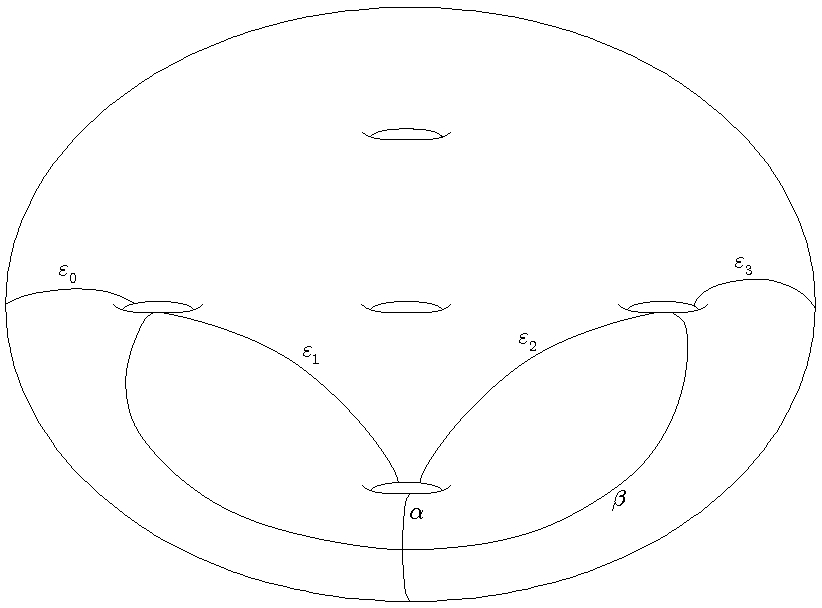
Let $\alpha$ and $\beta$ be two nonseparating curves in $S_{1}$ that are spherical-Farey neighbours, and $N(\alpha,\beta)$ be their closed regular neighbourhood. Then $N(\alpha,\beta)$ is homeomorphic to a genus zero surface with four boundary components. Let $\varepsilon_{0}$ , $\varepsilon_{1}$ , $\varepsilon_{2}$ , $\varepsilon_{3}$ be the boundary curves of $N(\alpha,\beta)$ . We say $\varepsilon_{i}$ and $\varepsilon_{j}$ are connected outside of $N(\alpha,\beta)$ , if there exists a proper arc in $S_{1}\backslash\mathrm{int}(N(\alpha,\beta))$ with one endpoint in $\varepsilon_{i}$ and another in $\varepsilon_{j}$ .

Remark 3.5.

If $\varepsilon_{i}$ is a nonseparating curve, it has to be connected outside of $N(\alpha,\beta)$ to at least one other $\varepsilon_{j}$ (with $i\neq j$ ), since otherwise there would not exist any curve intersecting $\varepsilon_{i}$ exactly once, and thus $\varepsilon_{i}$ would not be nonseparating.

We say $\alpha$ and $\beta$ are of type A if $\varepsilon_{i}$ is a nonseparating curve for all $i$ and $\varepsilon_{i}$ is connected outside of $\Sigma_{\alpha,\beta}$ to $\varepsilon_{j}$ for all $i,j\in\{0,1,2,3\}$ . See Figure 3.

Remark 3.6.

Remember that while $\pi_{\mathcal{HT}}$ is an edge-preserving map it is not alternating. Also, $\pi_{\mathcal{C}}$ has the property that if $\alpha$ and $\beta$ are disjoint nonseparating curves, then $i(\pi_{\mathcal{C}}(\alpha),\pi_{\mathcal{C}}(\beta))=0$ , since forgetting the punctures only affects the connected components of $S\backslash\{\alpha,\beta\}$ by possibly transforming one of them into a cylinder.

Lemma 3.7.

Let $\alpha$ and $\beta$ be two nonseparating curves in $S_{1}$ that are spherical-Farey neighbours of type A. Then $i(\psi(\alpha),\psi(\beta))\neq 0\neq i(\widetilde{\psi}(\alpha),\widetilde{\psi}(\beta))$ .

Proof.

This proof is divided in three parts: the first proves that $\psi(\alpha)\neq\psi(\beta)$ , the second proves that $\widetilde{\psi}(\alpha)\neq\widetilde{\psi}(\beta)$ , and finally the third proves that $i(\psi(\alpha),\psi(\beta))\neq 0\neq i(\widetilde{\psi}(\alpha),\widetilde{\psi}(\beta))$ .
First part: Since $\alpha$ and $\beta$ are of type A, we can always find curves $\gamma$ and $\delta$ such that:

•

$i(\alpha,\gamma)=i(\beta,\delta)=1$ .
•

$i(\alpha,\delta)=i(\beta,\gamma)=i(\gamma,\delta)=0$ .
•

There exists a multicurve $M$ of cardinality $g-2$ such that $C_{1}=\{\alpha,\delta\}\cup M$ , $C_{2}=\{\beta,\gamma\}\cup M$ and $C_{0}=\{\gamma,\delta\}\cup M$ are cut systems.

See Figure 4 for a way to obtain them.

Then $C_{1}$ , $C_{2}\in\mathcalligra{lk}\hskip 3.41418pt(C_{0})$ and $C_{1}\nsim_{C_{0}}C_{2}$ , so by definition and Lemma 2.4 $\phi(C_{1}),\phi(C_{2})\in\mathcalligra{lk}\hskip 3.41418pt(\phi(C_{0}))$ and $\phi(C_{1})\nsim_{\phi(C_{0})}\phi(C_{2})$ ; by Remark 1.3 $\phi(C_{1})$ and $\phi(C_{2})$ share exactly $g-2$ curves, thus $\psi(\alpha)\neq\psi(\beta)$ .
Second part: Using the cut systems $C_{1}$ , $C_{2}$ and $C_{0}$ from the first part of this proof, we can then apply Corollary 3.2, thus getting that $\widetilde{\psi}(\alpha)$ is disjoint from $\widetilde{\psi}(\delta)$ while $i(\widetilde{\psi}(\beta),\widetilde{\psi}(\delta))=1$ . Then $\widetilde{\psi}(\alpha)\neq\widetilde{\psi}(\beta)$ .
Third part: Let $\widetilde{P}$ be a multicurve such that $P_{1}=\widetilde{P}\cup\{\alpha\}$ and $P_{2}=\widetilde{P}\cup\{\beta\}$ are pants decompositions such that for $i=1,2$ , any two curves of $P_{i}$ do not separate the surface (see Figure 5 for an example). By Lemma 3.4 then $\widetilde{\psi}(P_{1})$ and $\widetilde{\psi}(P_{2})$ are pants decompositions of $S_{1}$ and, by the above paragraph, will differ in exactly one curve, $\widetilde{\psi}(\alpha)$ and $\widetilde{\psi}(\beta)$ , meaning that they are contained in a complexity-one subsurface of $S_{1}$ ; given that by the second part of the proof, these two curves are different and yet they are contained in a subsurface of complexity one, we have that $i(\widetilde{\psi}(\alpha),\widetilde{\psi}(\beta))\neq 0$ . Given that $\widetilde{\psi}=\pi_{\mathcal{C}}\circ\psi$ , by Remark 3.6 we have that $i(\psi(\alpha),\psi(\beta))\neq 0$ . ∎

A halving multicurve of a surface $S=S_{g,n}$ is a multicurve $H$ whose elements are nonseparating curves on $S$ such that: $S\backslash H=Q_{1}\sqcup Q_{2}$ , with $Q_{1}$ and $Q_{2}$ homeomorphic to $S_{0,n_{1}}$ and $S_{0,n_{2}}$ respectively, and $n_{1}+n_{2}=2(g+1)+n$ . Note that a halving multicurve has exactly $g+1$ elements.
We define a cutting halving multicurve as a halving multicurve such that any $g$ elements of it form a cut system. Note that there exist halving multicurves that are not cutting halving multicurves, see Figure 6 for an example.

Figure 6: An example of a halving multicurve that is not a cutting halving multicurve.

Lemma 3.8.

If $H$ is a cutting halving multicurve of $S_{1}$ , then $\psi(H)$ and $\widetilde{\psi}(H)$ are cutting halving multicurves of $S_{2}$ and $S_{1}$ respectively.

Proof.

Since $H$ is a cutting halving multicurve of $S_{1}$ then, by a repeated use of Lemma 3.1 and Corollary 3.2, $\psi(H)$ and $\widetilde{\psi}(H)$ will contain $g+1$ elements and any $g$ elements of $\psi(H)$ and $\widetilde{\psi}(H)$ will form cut systems. Therefore $S_{2}\backslash\psi(H)$ and $S_{1}\backslash\widetilde{\psi}(H)$ will have two connected components, each of genus zero; thus $\psi(H)$ and $\widetilde{\psi}(H)$ are cutting halving multicurves of $S_{2}$ and $S_{1}$ respectively. ∎

Lemma 3.9.

Let $\alpha$ and $\beta$ be two disjoint nonseparating curves such that $S_{1}\backslash\{\alpha,\beta\}$ is disconnected. Then $\psi(\alpha)$ and $\psi(\beta)$ are disjoint in $S_{2}$ and $\widetilde{\psi}(\alpha)$ and $\widetilde{\psi}(\beta)$ are disjoint in $S_{1}$ .

Proof.

We claim $\psi(\alpha)\neq\psi(\beta)$ and $\widetilde{\psi}(\alpha)\neq\widetilde{\psi}(\beta)$ .
Given the conditions, let $\gamma$ be a nonseparating curve such that $\beta$ and $\gamma$ are spherical-Farey neighbours of type A, $\alpha$ and $\gamma$ are disjoint, and $S_{1}\backslash\{\alpha,\gamma\}$ is connected; then, by Lemmas 3.1, 3.7 and Corollary 3.2, $i(\psi(\alpha),\psi(\gamma))=i(\widetilde{\psi}(\alpha),\widetilde{\psi}(\gamma))=0$ and $i(\psi(\beta),\psi(\gamma))\neq 0\neq i(\widetilde{\psi}(\beta),\widetilde{\psi}(\gamma))$ . Therefore $\psi(\alpha)\neq\psi(\beta)$ and $\widetilde{\psi}(\alpha)\neq\widetilde{\psi}(\beta)$ .
We claim $i(\psi(\alpha),\psi(\beta))=i(\widetilde{\psi}(\alpha),\widetilde{\psi}(\beta))=0$ .
Let $H$ be a cutting halving multicurve in $S_{1}$ such that $\alpha$ is contained in $S_{1}^{\prime}$ and $\beta$ is contained in $S_{1}^{\prime\prime}$ , where $S_{1}^{\prime}$ and $S_{1}^{\prime\prime}$ are the connected components of $S_{1}\backslash H$ , and also such that $S_{1}\backslash\{\alpha,\gamma\}$ and $S_{1}\backslash\{\beta,\gamma\}$ are connected for all $\gamma\in H$ . By Lemma 3.8 $\psi(H)$ is a cutting halving multicurve; let $S_{2}^{\prime}$ and $S_{2}^{\prime\prime}$ be the corresponding connected components of $S_{2}\backslash\psi(H)$ . See Figure 7 for examples. By construction $\psi(\alpha)$ and $\psi(\beta)$ are disjoint from every element in $\psi(H)$ , so they are curves contained in $S_{2}\backslash\psi(H)$ .
If $\psi(\alpha)$ and $\psi(\beta)$ are in different connected components of $S_{2}\backslash\psi(H)$ then they are disjoint. So, suppose (without loss of generality) that both representatives are in $S_{2}^{\prime\prime}$ .
Let $M$ be a multicurve of $S_{1}$ with the following properties.

1.

Every element of $M$ is also a curve contained in $S_{1}^{\prime\prime}$ and $S_{1}\backslash\{\gamma,\delta\}$ is connected for all $\gamma,\delta\in M$ .
2.

$S_{1}\backslash\{\gamma,\delta\}$ is connected for all $\gamma\in M$ and all $\delta\in H$ .
3.

For all $\gamma\in M$ , $\beta$ and $\gamma$ are spherical-Farey neighbours of type A.
4.

For all $\gamma\in M$ , $S_{1}\backslash\{\alpha,\gamma\}$ is connected.
5.

$M$ has $g-2$ elements.

See Figure 7 for an example. By Lemma 3.1, $\psi(M)$ satisfy conditions 1, 2, 4 and 5; also, by Lemma 3.7, we have that for all $\gamma\in M$ , $i(\psi(\beta),\psi(\gamma))\neq 0$ . This implies that every element of $\psi(M)$ is a curve contained in $S_{2}^{\prime\prime}$ ; thus $\psi(\gamma)$ intesects $\psi(\beta)$ at least twice for all $\gamma\in M$ (since $S_{2}^{\prime\prime}$ has genus zero, every curve contained in it is separating in $S_{2}^{\prime\prime}$ ).

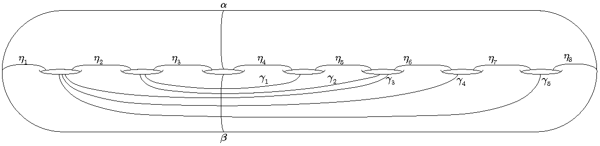
Let $U$ and $V$ be the connected components of $S_{2}^{\prime\prime}\backslash\{\psi(\alpha)\}$ .
Now, we prove by contradiction that the elements of $\psi(M)$ are either all in $U$ or all in $V$ : Let $\gamma,\gamma^{\prime}\in M$ be such that $\psi(\gamma)$ is contained in $U$ and $\psi(\gamma^{\prime})$ is contained in $V$ . Then we can always find a curve $\delta$ contained in $S_{1}^{\prime\prime}$ such that the elements of $\{\gamma,\delta\}$ and of $\{\gamma^{\prime},\delta\}$ satisfy the conditions of Lemma 3.7, and such that $S_{1}\backslash\{\delta,\delta^{\prime}\}$ is connected for all $\delta^{\prime}\in H\cup\{\alpha\}$ . This implies $i(\psi(\gamma),\psi(\delta))\neq 0\neq i(\psi(\gamma^{\prime}),\psi(\delta))$ , and that $\psi(\delta)$ has to be either in $U$ or $V$ . These two conditions together imply that $\psi(\delta)$ is contained in both $U$ and $V$ , which is a contradiction.
Therefore, $\psi(M)$ consists of $g-2$ nonseparating curves, no two of which separate $S_{2}$ , and (up to relabelling) all these nonseparating curves are disjointly contained in $U$ . But $U$ can have at most $g-3$ nonseparating (in $S_{2}$ ) curves that no pair of which separates $S_{2}$ (this number is actually the greatest possible cardinality of a punctured pants decomposition of $U$ ); so we have found a contradiction and thus $\psi(\alpha)$ and $\psi(\beta)$ are in different connected components and then $i(\psi(\alpha),\psi(\beta))=0$ .
By Remark 3.6, since $i(\psi(\alpha),\psi(\beta))=0$ , then $i(\widetilde{\psi}(\alpha),\widetilde{\psi}(\beta))=0$ . ∎

Thus, by using Lemmas 3.1, 3.9 and Corollary 3.2, we obtain the following corollary.

Corollary 3.10.

$\psi$ and $\widetilde{\psi}$ preserve both disjointness and intersection $1$ .

3.2 Inducing $\widehat{\psi}:\mathcal{C}(S_{1})\rightarrow\mathcal{C}(S_{1})$

To extend $\widetilde{\psi}$ , we proceed in the same way as Irmak in [8], using chains and the fact that every separating curve in $S_{1}$ is the boundary curve of a closed neighbourhood of a chain.
Using Lemmas 3.1, 3.9 and Corollary 3.2, we obtain the following lemma.

Lemma 3.11.

If $X$ is a chain of length $k$ , then $\psi(X)$ and $\widetilde{\psi}(X)$ are chains of length $k$ .

Since $S_{1}$ is a closed surface, then every separating curve $\alpha$ on $S_{1}$ can be characterized as the boundary curve of a closed regular neighbourhood of a chain $X_{\alpha}$ . See Figure 8 for an example. We call $X_{\alpha}$ a defining chain of $\alpha$ . Recall that every defining chain of a separating curve always has even cardinality, $2k$ , and its closed regular neighbourhood will then have genus $k$ .

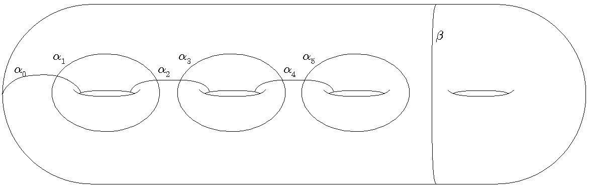
Lemma 3.12.

Let $\beta_{1}$ and $\beta_{2}$ be separating curves in $S_{1}$ , and $X_{1}$ and $X_{2}$ be defining chains of $\beta_{1}$ and $\beta_{2}$ respectively. If $\beta_{1}=\beta_{2}$ , then either every element of $X_{1}$ is disjoint from every element of $X_{2}$ and viceversa, or every curve in $X_{1}$ intersects at least one curve in $X_{2}$ and viceversa.

Proof.

Since every element in $X_{1}$ and $X_{2}$ is by definition disjoint from $\beta=\beta_{1}=\beta_{2}$ , then all the elements in $X_{1}$ are contained in the same connected component of $S_{1}\backslash\{\beta\}$ , and analogously with all the elements of $X_{2}$ . If the elements of $X_{2}$ are in a different connected component from those of $X_{1}$ then every element of $X_{1}$ is disjoint from every element of $X_{2}$ and viceversa. If the elements of $X_{2}$ are in the same connected component as those of $X_{1}$ , since $X_{1}$ fills its regular neighbourhood we have that every curve in $X_{1}$ intersects at least one curve in $X_{2}$ and viceversa. ∎

To extend the definition of $\widetilde{\psi}$ to $\mathcal{C}(S)$ , we define $\widehat{\psi}$ as follows: If $\alpha$ is a nonseparating curve, then $\widehat{\psi}(\alpha)=\widetilde{\psi}(\alpha)$ ; if $\alpha$ is a separating curve, let $X_{\alpha}$ be a defining chain of $\alpha$ and then we define $\widehat{\psi}(\alpha)$ as the boundary curve of a regular neighbourhood of $\widetilde{\psi}(X_{\alpha})$ . This makes sense given that the regular neighbourhoods of $X_{\alpha}$ are all isotopic, and thus the boundary curves of any two regular neighbourhoods are isotopic.

Lemma 3.13.

The map $\widehat{\psi}$ is well-defined.

Proof.

Let $\alpha$ be a separating curve and $X_{1}$ and $X_{2}$ be two defining chains of $\alpha$ . We divide this proof in two parts, depending on whether $X_{1}$ and $X_{2}$ are in the same connected component of $S_{1}\backslash\{\alpha\}$ or not.
Part 1: If $X_{1}$ and $X_{2}$ are in two different connected components, then due to Corollary 3.10 we have that every element in $\widehat{\psi}(X_{1})=\widetilde{\psi}(X_{1})$ will be disjoint from every element in $\widehat{\psi}(X_{2})=\widetilde{\psi}(X_{2})$ ; now, if $X_{1}$ (and thus also $\widehat{\psi}(X_{1})$ ) has length $2k$ , then $X_{2}$ (and thus also $\widehat{\psi}(X_{2})$ ) has length $2(g-k)$ . If we cut $S_{1}$ along the boundary curve of the regular neighbourhood of $\widehat{\psi}(X_{1})$ , we obtain a surface $S_{1}^{\prime}$ that has two connected components, one of genus $k$ and another of genus $g-k$ . If we cut $S_{1}^{\prime}$ along the boundary curve of a regular neighbourhood of $\widehat{\psi}(X_{2})$ (which means we are cutting $S_{1}^{\prime}$ in the connected component of genus $g-k$ ), we obtain a surface with three connected components: one of genus $k$ (since it is where the elements of $\widehat{\psi}(X_{1})$ are contained), one of genus $g-k$ (since it is where the elements of $\widehat{\psi}(X_{2})$ are contained), and an annulus. Therefore the two boundary curves of the regular neighbourhoods are isotopic, i.e. $\widehat{\psi}(\alpha)$ is well defined for these two chains.
Part 2: If $X_{1}$ and $X_{2}$ are in the same connected component, then we can find a defining chain $X_{3}$ on the other connected component such that the pairs $(X_{1},X_{3})$ and $(X_{2},X_{3})$ satisfy the conditions of the previous part, so the boundary curves of the regular neighbourhoods of the chains $(\widehat{\psi}(X_{1}),\widehat{\psi}(X_{3}))$ and $(\widehat{\psi}(X_{2}),\widehat{\psi}(X_{3}))$ are isotopic. Therefore $\widehat{\psi}(\alpha)$ is well defined. ∎

Now we prove that $\widehat{\psi}$ is an edge-preserving map, so that we can apply Theorem A from [7].

Lemma 3.14.

$\widehat{\psi}$ is an edge-preserving map.

Proof.

What we must prove is that given $\alpha$ and $\beta$ two disjoint curves, then $\widehat{\psi}(\alpha)$ and $\widehat{\psi}(\beta)$ are disjoint. If both $\alpha$ and $\beta$ are nonseparating curves, then we get the result from Corollary 3.10. If $\alpha$ is nonseparating and $\beta$ is separating, let $X$ be a defining chain of $\beta$ such that $\alpha\in X$ . Then by definition $\widehat{\psi}(\alpha)$ is disjoint from $\widehat{\psi}(\beta)$ .
If $\alpha$ and $\beta$ are both separating, then we can always find two disjoint defining chains $X_{\alpha}$ and $X_{\beta}$ of $\alpha$ and $\beta$ respectively. Then by the two previous cases, every element of $\widehat{\psi}(X_{\alpha})$ is disjoint from every element of $\widehat{\psi}(X_{\beta})\cup\{\widehat{\psi}(\beta)\}$ and every element of $\widehat{\psi}(X_{\beta})$ is disjoint from every element of $\widehat{\psi}(X_{\alpha})\cup\{\widehat{\psi}(\alpha)\}$ . Since by definition $\widehat{\psi}(\alpha)$ is the boundary curve of a regular neighbourhood of $\widehat{\psi}(X_{\alpha})$ , if $\widehat{\psi}(\beta)$ and $\widehat{\psi}(\alpha)$ were to intersect each other, $\widehat{\psi}(\beta)$ would have to intersect at least one element of $\widehat{\psi}(X_{\alpha})$ ; thus $i(\widehat{\psi}(\beta),\widehat{\psi}(\alpha))=0$ .
To prove that $\widehat{\psi}(\alpha)\neq\widehat{\psi}(\beta)$ , let $X_{1}$ and $X_{2}$ be chains such that $X_{1}$ is a defining chain of $\alpha$ and $X_{1}\cup X_{2}$ is a defining chain of $\beta$ . Thus $\widehat{\psi}(X_{1})$ and $\widehat{\psi}(X_{1}\cup X_{2})$ are defining chains of $\widehat{\psi}(\alpha)$ and $\widehat{\psi}(\beta)$ respectively. This implies that there exists (by the first case) an element in $\widehat{\psi}(X_{1}\cup X_{2})$ that is disjoint from every element in $\widehat{\psi}(X_{1})$ , and another element in $\widehat{\psi}(X_{1}\cup X_{2})$ that intersects at least one element in $\widehat{\psi}(X_{1})$ (this happens since $\widehat{\psi}|_{\mathcal{G}(S_{1})}=\widetilde{\psi}$ and we can apply Corollary 3.10). Then by Lemma 3.12, $\widehat{\psi}(\alpha)\neq\widehat{\psi}(\beta)$ . Therefore they are disjoint. ∎

Now, for the sake of completeness, we first cite Theorem A from [7] and then finalize with the proof of Theorem C:

Theorem (A in [7]).

Let $S_{1}=S_{g_{1},n_{1}}$ and $S_{2}=S_{g_{2},n_{2}}$ be two orientable surfaces of finite topological type such that $g_{1}\geq 3$ , and $\kappa(S_{2})\leq\kappa(S_{1})$ ; let also $\varphi:\mathcal{C}(S_{1})\rightarrow\mathcal{C}(S_{2})$ be an edge-preserving map. Then, $S_{1}$ is homeomorphic to $S_{2}$ and $\varphi$ is induced by a homeomorphism $S_{1}\rightarrow S_{2}$ .

Proof of Theorem C: We apply Theorem A from [7] to $\widehat{\psi}$ , obtaining an element $h$ of $\mathrm{Mod}^{*}(S_{1})$ that induces it. Since $h|_{\mathcal{G}(S_{1})}=\widehat{\psi}|_{\mathcal{G}(S_{1})}=\widetilde{\psi}$ , we have that (by Corollary 3.2) for every cut system $C=\{\alpha_{1},\ldots,\alpha_{g}\}$ in $S_{1}$ , $\widetilde{\phi}(C)=\{h(\alpha_{1}),\ldots,h(\alpha_{g})\}$ . Therefore $h$ induces $\widetilde{\phi}$ .

4 Proof of Corollary D

To prove Corollary D, we first prove a consequence of Theorem C:

Corollary 4.1.

Let $S=S_{g,0}$ be an orientable closed surface of finite topological type of genus $g\geq 3$ , and $\phi:\mathcal{HT}(S)\rightarrow\mathcal{HT}(S)$ be an edge-preserving alternating map. Then $\phi$ is induced by a homeomorphism of $S$ .

Proof.

By supposing $S=S_{1}=S_{2}$ we have that $\pi_{\mathcal{HT}}$ is the identity, and by applying Theorem C we obtain that $\widetilde{\phi}=\phi$ is induced by a homeomorphism. ∎

Proof of Corollary D.

Let $\phi:\mathcal{HT}(S_{1})\rightarrow\mathcal{HT}(S_{2})$ be an isomorphism. We first prove that it is alternating. By Lemma 2.4 we have that for all cut systems $C$ in $S_{1}$ , $\phi$ preserves the colours in $\mathcalligra{lk}\hskip 3.41418pt(C)$ . Applying the same lemma to $\phi^{-1}$ , we have that two cut systems in $\mathcalligra{lk}\hskip 3.41418pt(C)$ are in the same colour if and only if their images are in the same colour in $\mathcalligra{lk}\hskip 3.41418pt(\phi(C))$ . This implies that $\phi$ is an alternating map.
Given that $\phi$ and $\phi^{-1}$ are isomorphisms, then they are also edge-preserving maps, and by Theorem A applied to $\phi$ and $\phi^{-1}$ , we have that $g_{1}=g_{2}$ .
Now, let $S=S_{g,0}$ with $g\geq 3$ . To prove that $\mathrm{Aut}(\mathcal{HT}(S))$ is isomorphic to $\mathrm{Mod}^{*}(S)$ , we note there is a natural homomorphism:

$\Psi_{\mathcal{HT}(S)}:$	$\mathrm{Mod}^{*}(S)$	$\longrightarrow$	$\mathrm{Aut}(\mathcal{HT}(S))$
	$[h]$	$\mapsto$	$\varphi:\mathcal{HT}(S)$	$\rightarrow$	$\mathcal{HT}(S)$
			$\{\alpha_{1},\ldots,\alpha_{g}\}$	$\mapsto$	$\{h(\alpha_{1}),\ldots,h(\alpha_{g})\}$

Injectivity: If $h_{1}$ and $h_{2}$ are two homeomorphisms of $S$ such that $\Psi_{\mathcal{HT}(S)}([h_{1}])=\Psi_{\mathcal{HT}(S)}([h_{2}])$ , then the action of $h_{1}$ and $h_{2}$ on the nonseparating curves on $S$ would be exactly the same. Recalling that Schmutz-Schaller proved in [10] that $\mathrm{Aut}(\mathcal{G}(S))$ is isomorphic to $\mathrm{Mod}^{*}(S)$ , this implies that $h_{1}$ is isotopic to $h_{2}$ .
Surjectivity: If $\phi\in\mathrm{Aut}(\mathcal{HT}(S))$ , then (as was proved above) it is an edge-preserving alternating map. Thus, by Corollary 4.1 we have that $\phi$ is induced by a homeomorphism.
Therefore, $\mathrm{Aut}(\mathcal{HT}(S))$ is isomorphic to $\mathrm{Mod}^{*}(S)$ . ∎

References

[1] J. Aramayona. Simplicial embeddings between pants graphs. Geometriae Dedicata, 144 vol. 1, 115-128, (2010).
[2] B. Farb, D. Margalit. A primer on mapping class groups. Princeton University Press, (2011).
[3] W. J. Harvey. Geometric structure of surface mapping class groups. Homological Group Theory (Proc. Sympos., Durham, 1977), London Math. Soc. Lecture Notes Ser. 36, Cambridge University Press, Cambridge, 255-269, (1979).
[4] A. Hatcher, W. Thurston. A presentation for the mapping class group of a closed orientable surface. Topology, 19(3) p221-p237 (1980).
[5] J. Hernández Hernández. Combinatorial rigidity of complexes of curves and multicurves. Ph.D. thesis. Aix-Marseille Université, (2016).
[6] J. Hernández Hernández. Exhaustion of the curve graph via rigid expansions. Preprint, arXiv:1611.08010 [math.GT] (2016).
[7] J. Hernández Hernández. Edge-preserving maps of curve graphs. Preprint, arXiv:1611.08328 [math.GT] (2016).
[8] E. Irmak. Complexes of nonseparating curves and mapping class groups. Michigan Math. J., 81-110 54 No. 1 (2006).
[9] E. Irmak, M. Korkmaz. Automorphisms of the Hatcher-Thurston complex. Israel Journal of Math. 162 (2007).
[10] P. Schmutz-Schaller, Mapping class groups of hyperbolic surfaces and automorphism groups of graphs, Compositio Math. 122 (2000).
[11] K. J. Shackleton. Combinatorial rigidity in curve complexes and mapping class groups. Pacific Journal of Mathematics, 230, No. 1 (2007).
[12] B. Wajnryb. An elementary approach to the mapping class group of a surface. Geom. Top. 3 (1999).

Alternating maps on Hatcher-Thurston graphs

Abstract

Introduction

Theorem A.

Question B.

Theorem C.

Corollary D.

1 Preliminaries and properties

Remark 1.1.

Lemma 1.2 ([12]).

1.1 Properties of ℋ​𝒯​(S)\mathcal{HT}(S)

Remark 1.3.

Lemma 1.4 ([9]).

Lemma 1.5.

Proof.

Lemma 1.6.

Proof.

2 Proof of Theorem A

Lemma 2.1.

Proof.

Lemma 2.2.

Proof.

Remark 2.3.

Lemma 2.4.

Proof.

Proof of Theorem A.

3 Proof of Theorem C

3.1 Inducing ψ:𝒢⁡(S1)→𝒢⁡(S2)\psi:\mathcal{G}(S_{1})\rightarrow\mathcal{G}(S_{2}) and ψ~:𝒢⁡(S1)→𝒢⁡(S1)\widetilde{\psi}:\mathcal{G}(S_{1})\rightarrow\mathcal{G}(S_{1})

Lemma 3.1.

Proof.

Corollary 3.2.

Proof.

Corollary 3.3.

Lemma 3.4.

Proof.

Remark 3.5.

Remark 3.6.

Lemma 3.7.

Proof.

Lemma 3.8.

Proof.

Lemma 3.9.

Proof.

Corollary 3.10.

3.2 Inducing ψ^:𝒞⁡(S1)→𝒞⁡(S1)\widehat{\psi}:\mathcal{C}(S_{1})\rightarrow\mathcal{C}(S_{1})

Lemma 3.11.

Lemma 3.12.

Proof.

Lemma 3.13.

Proof.

Lemma 3.14.

Proof.

Theorem (A in [7]).

4 Proof of Corollary D

Corollary 4.1.

Proof.

Proof of Corollary D.

References

1.1 Properties of $\mathcal{HT}(S)$

3.1 Inducing $\psi:\mathcal{G}(S_{1})\rightarrow\mathcal{G}(S_{2})$ and $\widetilde{\psi}:\mathcal{G}(S_{1})\rightarrow\mathcal{G}(S_{1})$

3.2 Inducing $\widehat{\psi}:\mathcal{C}(S_{1})\rightarrow\mathcal{C}(S_{1})$