跳到论文正文
W Papers独立论文阅读器 arXiv:1611.09972 论文正文 计算阅读时间 · 0%
引用这篇论文根据当前论文元数据生成,正式投稿前建议核对。


License: arXiv.org perpetual non-exclusive license
arXiv:1611.09972v4 [stat.ME] 18 Jun 2019

Nonparametric regression with adaptive truncation via a convex hierarchical penalty

Asad Haris    Ali Shojaie    Noah Simon Affiliation: Department of Biostatistics, University of Washington-Seattle
Abstract

We consider the problem of nonparametric regression with a potentially large number of covariates. We propose a convex, penalized estimation framework that is particularly well-suited for high-dimensional sparse additive models and combines appealing features of finite basis representation and smoothing penalties. In the case of additive models, a finite basis representation provides a parsimonious representation for fitted functions but is not adaptive when component functions posses different levels of complexity. In contrast, a smoothing spline type penalty on the component functions is adaptive but does not provide a parsimonious representation. Our proposal simultaneously achieves parsimony and adaptivity in a computationally efficient way. We demonstrate these properties through empirical studies and show that our estimator converges at the minimax rate for functions within a hierarchical class. We further establish minimax rates for a large class of sparse additive models. We also develop an efficient algorithm that scales similarly to the lasso with the number of covariates and sample size.

Keywords – Additive model; High-dimensional data; Minimax estimation; Nonparametric regression; Sparsity.

1 Introduction and motivation

Consider univariate nonparametric function estimation from observations {(xi,yi)∈ℝ2:i=1,…,n}\{(x_{i},y_{i})\in\mathbb{R}^{2}:i=1,\ldots,n\}. Assume that yi=f⁡(xi)+εiy_{i}=f(x_{i})+\varepsilon_{i} (i=1,…,ni=1,\ldots,n), where εi\varepsilon_{i} are independent, mean zero, sub-Gaussian random variables. There are many proposals for estimating ff, including local polynomials (Stone, 1977), kernel smoothing (Nadaraya, 1964; Watson, 1964), and splines (Wahba, 1990). To begin, we focus on basis expansion estimators, also known as projection estimators (Čencov, 1962), which are widely used, and arguably the simplest.

Let y=(y1,…,yn)⊤∈ℝn{y}=(y_{1},\ldots,y_{n})^{\top}\in\mathbb{R}^{n} and x=(x1,…,xn)⊤∈ℝn{x}=(x_{1},\ldots,x_{n})^{\top}\in\mathbb{R}^{n} be the response and covariate vectors. For v∈ℝn{v}\in\mathbb{R}^{n}, let ‖v‖n2=n−1​∑i=1nvi2\|{v}\|_{n}^{2}=n^{-1}\sum_{i=1}^{n}v_{i}^{2} be a modified ℓ2\ell_{2}-norm, referred to as the empirical norm. Projection estimators are solutions to linear regression problems based on a set of basis functions (ψk)k=1∞(\psi_{k})_{k=1}^{\infty}, with a truncation level KK. More specifically, let ΨK∈ℝn×K{\Psi}_{K}\in\mathbb{R}^{n\times K} be the n×Kn\times K matrix with entries ΨK⁡(i,k)=ψk​(xi){\Psi}_{K(i,k)}=\psi_{k}(x_{i}) (k=1,…,K;i=1,…,nk=1,\ldots,K;i=1,\ldots,n). The basis expansion estimate of ff is given by f^=∑k=1Kβ^kproj​ψk\widehat{f}=\sum_{k=1}^{K}\widehat{\beta}^{\text{proj}}_{k}\psi_{k}, where

β^proj=argminβ∈ℝK​12​‖y−ΨK​β‖n2.\widehat{{\beta}}^{\text{proj}}=\underset{{\beta}\in\mathbb{R}^{K}}{\operatorname{argmin}}\ \frac{1}{2}\left\|{y}-{\Psi}_{K}{\beta}\right\|_{n}^{2}. (1)

To asymptotically balance bias and variance, K≡KnK\equiv K_{n} is allowed to vary with nn. Unfortunately, choosing the truncation level KK can be difficult in practice; it depends on the variance of εi\varepsilon_{i}, properties of ff such as smoothness, and the choice of basis functions. Usually, KK is chosen via split-sample validation. The challenge of tuning KK becomes more evident in multivariate problems, which we describe next, and is one of our main motivations.

Multivariate additive models (Hastie et al., 2009) easily follow from projection estimators, where each xi=(xi​1,…,xi​p)⊤{x}_{i}=\left(x_{i1},\ldots,x_{ip}\right)^{\top} is now a pp-vector, and the true underlying model is believed to be of the form yi=∑j=1pfj​(xi​j)+εi​(i=1,…,n).y_{i}=\sum_{j=1}^{p}f_{j}\left(x_{ij}\right)+\varepsilon_{i}\ (i=1,\ldots,n). The components fjf_{j} of this model can be estimated by using a basis expansion for each jj and solving

β^1A-proj,…,β^pA-proj=argminβj∈ℝKj​12​‖y−∑j=1pΨKjj​βj‖n2,\widehat{{\beta}}^{\text{A-proj}}_{1},\ldots,\widehat{{\beta}}^{\text{A-proj}}_{p}=\underset{{\beta}_{j}\in\mathbb{R}^{K_{j}}}{\operatorname{argmin}}\ \frac{1}{2}\Big\|y-\sum_{j=1}^{p}{\Psi}^{j}_{K_{j}}\beta_{j}\Big\|_{n}^{2}, (2)

where ΨKjj{\Psi}^{j}_{K_{j}} are KjK_{j} basis functions for feature jj and fjf_{j} is estimated as f^j=∑k=1Kjβ^j​kA-proj​ψk\widehat{f}_{j}=\sum_{k=1}^{K_{j}}\widehat{\beta}^{\text{A-proj}}_{jk}\psi_{k}.

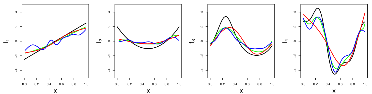
In practice, the same truncation level is used for each feature, Kj≡KK_{j}\equiv K, to reduce the number of tuning parameters. When fjf_{j} have widely different complexities, this leads to poor estimates. This limitation, which is illustrated by the simulation in Figure 1, becomes more hindering in higher dimensions, as pp increases. In high-dimensional problems, when p≫np\gg n, it is often assumed that fj≡0f_{j}\equiv 0 for many components. A popular choice is then to add a sparsity-inducing penalty to the basis expansion framework (Ravikumar et al., 2009) and solve

β^1SPAM,…,β^pSPAM=argminβj∈ℝK​12​‖y−∑j=1pΨKj​βj‖n2+λ​∑j=1p‖ΨKj​βj‖n.\widehat{\beta}^{\text{SPAM}}_{1},\ldots,\widehat{\beta}^{\text{SPAM}}_{p}=\underset{\beta_{j}\in\mathbb{R}^{K}}{\operatorname{argmin}}\ \frac{1}{2}\Big\|y-\sum_{j=1}^{p}{\Psi}^{j}_{K}\beta_{j}\Big\|_{n}^{2}+\lambda\sum_{j=1}^{p}\Big\|{\Psi}^{j}_{K}\beta_{j}\Big\|_{n}. (3)

In this manuscript, we propose a penalized estimation framework that penalizes function complexity, simultaneously selects the truncation level, and can be used to fit both univariate and multivariate additive models with or without sparsity. We present an extension for fully nonparametric multivariate settings, as well as a relaxed version, similar to the relaxed lasso (Meinshausen, 2007), which reduces the bias. While our univariate proposal is similar to (1), our additive proposal data-adaptively selects the truncation level for each feature, fjf_{j}. This improves the prediction accuracy and provides parsimonious estimates of fj{f}_{j}. We illustrate these advantages in a small simulation study with data yi=f1​(xi​1)+f2​(xi​2)+εi​(i=1,…,n)y_{i}=f_{1}(x_{i1})+f_{2}(x_{i2})+\varepsilon_{i}\ (i=1,\ldots,n) using f1,f2f_{1},f_{2} shown in Figure 1. We fit (2) using Kj≡KK_{j}\equiv K selected to optimize mean square error, and compare it to our relaxed proposal. Tuning parameters for our method also minimizes the mean square error. The results in Figure 1 clearly demonstrate the superior performance of our method, which has lower mean square error while maintaining parsimony. In particular, we estimate the linear term, f1f_{1}, by a linear function, whereas (2) uses an order 9 polynomial.

Refer to caption
Figure 1: Left: Plots of component functions f1f_{1} (Refer to caption) and f2f_{2} (Refer to caption). Middle: Minimum mean square errors as functions of nn for our proposal (Refer to caption) and (2) (Refer to caption). Right: Degrees of fitted polynomial as functions of nn: for our proposal, f^1\widehat{f}_{1} (Refer to caption) and f^2\widehat{f}_{2} (Refer to caption) are shown; for (2) both component functions have the same degree (Refer to caption). All results are averaged over 100 replications.

In addition to adaptability and parsimony, our proposal is computationally efficient and can work with thousands of observations and features. Moreover, its estimates attain minimax optimal rates under standard smoothness assumptions, for univariate, multivariate, and sparse additive models. The univariate estimator converges at rate n−2m/(2m+1)n^{-{2m}/{(2m+1)}} where mm is the degree of smoothness; similarly, the multivariate estimator attains the rate n−2m/(2m+p)n^{-{2m}/{(2m+p)}}. For sparse additive models, under a suitable compatibility condition, our estimator converges at rate max{sn−2m/(2m+1),slogp/n},\max\left\{sn^{-{2m}/{(2m+1)}},{s\log p}/{n}\right\}, where ss is the number of non-zero fjf_{j}; even without the compatibility condition, consistency is achieved at the rate max{sn−m/(2m+1),s(logp/n)1/2}\max\left\{sn^{-{m}/{(2m+1)}},s({\log p}/{n})^{1/2}\right\}.

2 Methodology

2.1 Motivation for adaptive truncation

Our proposal is motivated by the need to select the truncation levels in a data-driven manner. Let us first reconsider the simple projection estimator. The bias-variance tradeoff and parsimony of estimates f^j\widehat{f}_{j} in (2) are controlled by truncation levels KjK_{j}. While separately tuning KjK_{j} over each component function may be feasible in low dimensions, it quickly becomes infeasible for additive models, as the optimal truncation level requires searching over a pp-dimensional space.

To bypass the tuning of multiple truncation levels, Kj​(j=1,…,p)K_{j}(j=1,\ldots,p), one can instead use nn basis functions for each component, and consider a penalized version of the truncation estimator,

β^1proj-pen,…,β^pproj-pen=argminβj∈ℝn12∥y−∑j=1pΨnjβj∥n2+λ∑j=1pmax(k:βj​k≠0),\widehat{{\beta}}^{\text{proj-pen}}_{1},\ldots,\widehat{{\beta}}^{\text{proj-pen}}_{p}=\underset{{\beta}_{j}\in\mathbb{R}^{n}}{\operatorname{argmin}}\ \frac{1}{2}\Big\|y-\sum_{j=1}^{p}{\Psi}^{j}_{n}\beta_{j}\Big\|_{n}^{2}+\lambda\sum_{j=1}^{p}\operatorname{max}(k:\,\beta_{jk}\neq 0), (4)

where the truncation level for each feature is determined using the penalty max(k:βj​k≠0)\operatorname{max}(k:\beta_{jk}\neq 0). The estimator in (4) chooses the truncation level for each feature data-adaptively. However, the penalty in (4) is non-convex, so solving (4) becomes infeasible in moderate to high-dimensional problems. To mitigate this challenge, we formulate a convex problem using a novel penalty that can be seen as a convex relaxation of the penalty in (4).

Our approach is particularly suitable for basis functions that possess a natural hierarchy, that is, when (ψk)k=1∞\left(\psi_{k}\right)_{k=1}^{\infty} become increasingly complex for higher values of kk, as opposed to, say, natural splines, which rely on knot points. Examples of hierarchical basis functions include polynomial, trigonometric and wavelet basis functions; see the online Supplementary Material.

2.2 The univariate proposal

Consider again the projection estimator (1). As noted in Section 1, choosing the truncation level KK is key here: KK too small will result in large bias, while KK too large will over-inflate the variance. The bias and variance are balanced by taking K=O​{n1/(2​m+1)}K={O}\left\{n^{{1}/{(2m+1)}}\right\}, where mm relates to the smoothness of the underlying ff, and is unknown in practice. To circumvent this challenge, we use instead a complete basis with K=nK=n along with regularization to choose the truncation level. Our estimator is defined as

β^hier=argminβ∈ℝn12‖y−Ψnβ‖n2+λΩ(β),Ω(β)=∑k=1nwk‖Ψk:nβk:n‖n,\widehat{\beta}^{\text{hier}}=\underset{\beta\in\mathbb{R}^{n}}{\operatorname{argmin}}\ \frac{1}{2}\left\|y-\Psi_{n}\beta\right\|_{n}^{2}+\lambda\Omega\left(\beta\right),\quad\Omega\left({\beta}\right)=\sum_{k=1}^{n}w_{k}\left\|{\Psi}_{k:n}{\beta}_{k:n}\right\|_{n}, (5)

with wk=km−(k−1)mw_{k}=k^{m}-(k-1)^{m}. Here, Ψk:n{\Psi}_{k:n} denotes the submatrix of Ψn{\Psi}_{n} containing columns kk to nn, βk:n{\beta}_{k:n} is the subvector of β{\beta} containing entries kk to nn, and mm and λ\lambda are tuning parameters. The choice of weights wkw_{k} is theoretically motivated, and detailed in Section 5. Briefly, it defines a function class with desirable properties that allow us to establish convergence rates.

The hierarchical group lasso penalty Ω⁡(β)\Omega\left(\beta\right), will result in solutions β^hier\widehat{{\beta}}^{\text{hier}} with hierarchical sparsity: that is, if β^khier=0\widehat{\beta}^{\text{hier}}_{k}=0 for some kk, then β^hierk′=0\widehat{\beta}^{\text{hier}}_{k^{{}^{\prime}}}=0 for all k′>kk^{{}^{\prime}}>k. For sufficiently large λ\lambda, many entries of β^hier\widehat{\beta}^{\text{hier}} will be 00. For a given λ\lambda, we define the induced truncation level to be the minimal integer K≤nK\leq n such that β^khier=0\widehat{\beta}^{\text{hier}}_{k}=0 for all integers k>Kk>K. Unlike the simple basis expansion estimator (1), this truncation level is data-adaptive, not prespecified.

Equation (5) involves two tuning parameters, mm and λ\lambda. The parameter mm is analogous to the smoothness parameter in smoothing splines (Wahba, 1990), or the number of bounded derivatives used in simple projection estimator (Čencov, 1962). In practice, using m=2m=2 or 33 gives good results; this is similar to the use of cubic smoothing splines. On the other hand, λ\lambda determines the trade-off between goodness-of-fit and parsimony; a theoretically optimal λ\lambda-value is λ∝n−m/(2m+1)\lambda\propto n^{-{m}/{(2m+1)}}. Split-sample validation can be used to choose λ\lambda in practice.

As with the lasso, the regularization in (5) results in bias, which can reduce the overall mean square error. To reduce this bias, we can consider the relaxed version of our estimator in (5) as the simple basis expansion estimator with K=‖β^hier‖0K=\|\widehat{\beta}^{\text{hier}}\|_{0}, the truncation level selected by (5). This relaxed proposal is equivalent to using the penalty for selecting a truncation level. Therefore, in the univariate case, the relaxed estimator for a sequence of λ\lambda values would match the simple basis expansion estimator (1) for a sequence of KK values. However, the advantages of our penalty become more clear in the case of multivariate additive models, discussed next.

2.3 The additive proposal

Ideally, the additive projection estimator (2) is obtained by considering a different truncation level KjK_{j} for each feature. When pp is small, this can be achieved by using split-sample validation and searching over all combinations of Kj​(j=1,…,p)K_{j}(j=1,\ldots,p); however, the number of candidate models grows exponentially in pp and becomes quickly unwieldy. Often, a single K≡KjK\equiv K_{j} is used in practice, which can lead to some fjf_{j} estimates with too many degrees of freedom. As illustrated in Figure 1, using a single truncation level can lead to poor estimates.

Our proposal, which can be seen as a convex relaxation of (4), is designed to circumvent the above limitation of projection estimators in choosing the truncation level for models with multiple covariates. This differentiates our proposal from the projection estimator: in our framework, a single tuning parameter λ\lambda leads to different KjK_{j} for each fitted fjf_{j}.

Our additive framework is a direct extension of our univariate proposal (5). Specifically, we consider function estimates f^j=∑k=1nβ^j​kA-hier​ψk\widehat{f}_{j}=\sum_{k=1}^{n}\widehat{\beta}^{\text{A-hier}}_{jk}\psi_{k}, where

β^1A-hier,…,β^pA-hier=argminβj∈ℝn​12​‖y−∑j=1pΨnj​βj‖n2+λ​∑j=1pΩj​(βj),\widehat{{\beta}}^{\text{A-hier}}_{1},\ldots,\widehat{{\beta}}^{\text{A-hier}}_{p}=\underset{{\beta}_{j}\in\mathbb{R}^{n}}{\operatorname{argmin}}\ \frac{1}{2}\Big\|{y}-\sum_{j=1}^{p}{\Psi}^{j}_{n}{\beta}_{j}\Big\|_{n}^{2}+\lambda\sum_{j=1}^{p}\Omega_{j}\left({\beta}_{j}\right), (6)

and Ωj\Omega_{j} is the hierarchical group lasso penalty with weights wk=km−(k−1)mw_{k}=k^{m}-(k-1)^{m}:

Ωj(βj)=∑k=1nwk‖Ψk:njβj,k:n‖n.\Omega_{j}\left({\beta}_{j}\right)=\sum_{k=1}^{n}w_{k}\left\|{\Psi}^{j}_{k:n}{\beta}_{j,k:n}\right\|_{n}. (7)

The optimization problem (6) results in β^j\widehat{{\beta}}_{j} estimates that are hierarchically sparse for each jj. Specifically, for each jj, there is some minimal KjK_{j} such that β^j​kA-hier=0\widehat{\beta}^{\text{A-hier}}_{jk}=0 for all integers k>Kjk>K_{j}. Moreover, the major advantage of (6) is that the induced truncation level is feature-wise adaptive, with a different KjK_{j} for each feature jj. Additionally, as in the univariate setting, we can define a relaxed version of our estimator by fitting (2), where KjK_{j} is now determined by (6). As a result, our framework balances goodness-of-fit and parsimony for each feature individually, without requiring an exhaustive search. This is a major advantage over simple projection estimators.

The advantage of our method over simple projection estimators becomes more evident in high dimensions, when p≫np\gg n. For instance, the popular estimator of Ravikumar et al., (3), is generally obtained by using a single truncation level, which, as noted above, can result in poor estimates. Similar to their proposal, our sparse additive framework encourages feature-wise sparsity using a group lasso penalty (Yuan & Lin, 2006), and is defined as

β^1S-hier,…,β^pS-hier=argminβj∈ℝn​12​‖y−∑j=1pΨnj​βj‖2+λ2​∑j=1pΩj​(βj)+λ​∑j=1p‖Ψnj​βj‖n,\widehat{{\beta}}^{\text{S-hier}}_{1},\ldots,\widehat{{\beta}}^{\text{S-hier}}_{p}=\underset{{\beta}_{j}\in\mathbb{R}^{n}}{\operatorname{argmin}}\ \frac{1}{2}\Big\|{y}-\sum_{j=1}^{p}{\Psi}^{j}_{n}{\beta}_{j}\Big\|_{2}+\lambda^{2}\sum_{j=1}^{p}\Omega_{j}\left({\beta}_{j}\right)+\lambda\sum_{j=1}^{p}\left\|{\Psi}^{j}_{n}{\beta}_{j}\right\|_{n}, (8)

with Ωj​(βj)\Omega_{j}\left({\beta}_{j}\right) given in (7). We can again define a relaxed version which fits (2) with sparsity and KjK_{j} selected by (8). An important feature of the optimization problem (8) is that the tuning parameters for the two penalty terms λ\lambda and λ2\lambda^{2} are linked. This link is theoretically justified in Section 4. Briefly, for an oracle λ\lambda, the choice of tuning parameters in (8) gives rate-optimal estimates. In practice, while this formulation gives good predictive performance in many cases, in other cases tuning sparsity and smoothness separately leads to strong predictive performance. Our numerical experiments in Section 5 and 6 corroborate this finding.

As with β^jSPAM\widehat{{\beta}}^{\text{SPAM}}_{j} in (3), for sufficiently large λ\lambda, our proposal gives a sparse solution with most β^jS-hier≡0\widehat{{\beta}}^{\text{S-hier}}_{j}\equiv 0. The two estimators differ, however, in their nonzero estimates: non-zero β^jS-hier\widehat{{\beta}}^{\text{S-hier}}_{j} are hierarchically sparse, with a data-driven feature-specific induced truncation level, whereas nonzero β^jSPAM\widehat{{\beta}}^{\text{SPAM}}_{j} in (3) all have the same complexity. This additional flexibility of our methodology proves critical in high dimensions, and is achieved without paying a price in computational or sample complexity. Moreover, with the tuning parameters in (8), this additional flexibility is in theory achieved with the same number of tuning parameters as Ravikumar et al.’s method.

2.4 Relationship to existing methods

The univariate framework of Section 2.2 builds upon existing penalized estimation methods. A popular choice is the smoothing spline estimator (Wahba, 1990), which sets (ψk)k=1n(\psi_{k})_{k=1}^{n} to nn natural splines with knots at the observed covariates x1,…,xnx_{1},\ldots,x_{n}; this estimator is found by minimizing ‖y−Ψ​β‖n2+2​λ​‖C1/2​β‖n2\|{y}-{\Psi}{\beta}\|_{n}^{2}+2\lambda\|C^{1/2}{\beta}\|_{n}^{2} over β∈ℝn\beta\in\mathbb{R}^{n}, using C∈ℝn×nC\in\mathbb{R}^{n\times n} and Cj,k=∫ψj(m/2+1/2)​(t)​ψk(m/2+1/2)​(t)​𝑑tC_{j,k}=\int\psi_{j}^{\left(m/2+1/2\right)}(t)\psi_{k}^{\left(m/2+1/2\right)}(t)\,dt with ψ(k)\psi^{(k)} denoting the kkth order derivative of ψ\psi. The smoothing spline eliminates the dependence on the truncation level and has an efficient-to-compute closed-form solution; but its estimated functions are piecewise polynomial splines of degree mm with nn knots. As a result, smoothing spline estimates are not parsimonious. To achieve more parsimonious estimates, Mammen & van de Geer (1997) use a data-driven approach to select the knots in spline functions. Their locally adaptive regression splines use the same natural spline basis and is found by minimizing ‖y−Ψ​β‖n2+2​λ​(m!)−1​‖D​β‖1,\|{y}-{\Psi}{\beta}\|_{n}^{2}+2\lambda(m!)^{-1}\|D{\beta}\|_{1}, over β∈ℝn\beta\in\mathbb{R}^{n}, using D∈ℝ(n−m−1)×nD\in\mathbb{R}^{(n-m-1)\times n} with Di,j=ψj(m)​(ti)−ψj(m)​(ti−1)D_{i,j}=\psi_{j}^{(m)}(t_{i})-\psi_{j}^{(m)}(t_{i-1}). This is closely related to the more computationally tractable trend filtering proposal (Kim et al., 2009; Tibshirani, 2014).

Table 1: Comparison of existing methods for sparse additive models.
PE SS/RKHS TF
 
Scalability
✓\checkmark Exact solution for univariate sub-problem; scales as O⁡(n​p​K)O(npK). ×\times No exact solution for univariate sub-problem; general convex solver scaling as O​{(n​p)3}O\{(np)^{3}\}. ×\times Inefficient beyond first order TF, particularly for high-dimensional and unequally spaced covariates.
 
Adaptability
×\times Smoothness controlled by basis expansion order, KK, fixed for all component functions. ✓ Smoothness controlled by smoothness norm, varied for component functions. ✓ Smoothness controlled by smoothness norm and number of knots, KK, varied for component functions.
 
Parsimony
✓\checkmark Component functions of order K≪nK\ll n expansions. ×\times Component functions of order nn expansions. ✓\checkmark Component functions have sparsity in number of knots.

Despite their appealing properties in the univariate setting, locally adaptive regression splines and trend filtering are computationally difficult to extend to high-dimensional sparse additive models; even for a single feature, neither estimator has a closed-form solution. Ravikumar et al.’s estimator (3) overcomes this difficulty by using a fixed truncation level for all pp components. As mentioned earlier, its main drawback is that all nonzero components of the additive model have the same complexity. The sparse partially linear additive model of Lou et al. (2016) partly mitigates this by setting some of the nonzero components to linear functions using a hierarchical penalty of the form ∑j=1pλ1​‖βj‖2+λ2​‖βj,−1‖2;\sum_{j=1}^{p}\lambda_{1}\|{\beta}_{j}\|_{2}+\lambda_{2}\|{\beta}_{j,-1}\|_{2}; here βj,1\beta_{j,1} is the coefficient of the linear term in the basis expansion, βj,−1=(βj,2,…,βj,K)⊤∈ℝK−1{\beta}_{j,-1}=(\beta_{j,2},\ldots,\beta_{j,K})^{\top}\in\mathbb{R}^{K-1}, and λ1\lambda_{1} and λ2\lambda_{2} are tuning parameters. The first term in the penalty sets all of the coefficients for the jjth feature to zero, whereas the second term only sets the K−1K-1 coefficients corresponding to higher-order terms to zero.

Our additive and sparse additive proposals of Section 2.3 generalize those of Ravikumar et al. (2009) and Lou et al. (2016). The first becomes a special case of (8) if the weights in (7) are set to w1=1​ and ​wk=0​ for ​k>1.w_{1}=1\text{ and }w_{k}=0\text{ for }k>1. Similarly, with an orthogonal design matrix, (ΨKj)⊤​ΨKj/n=IK​(j=1,…,p)({\Psi}_{K}^{j})^{\top}{\Psi}_{K}^{j}/n=I_{K}\ (j=1,\ldots,p), Lou et al.’s method is a special case of (8) with weights in (7) set to w1=w2=1​ and ​wk=0​ for ​k>2.w_{1}=w_{2}=1\text{ and }w_{k}=0\text{ for }k>2. Our theoretical analysis in Section 4.5 indicates that, in addition to the improved flexibility, our choice of weights (7) results in optimal rates of convergence.

There are other proposals for estimating sparse additive models, including extensions of trend-filtering and smoothing splines for additive models. Extensions of trend filtering were either not shown to be rate optimal (Petersen et al., 2016) or only shown to be so for low-dimensional additive models (Sadhanala & Tibshirani, 2018). These extensions are also computationally challenging beyond first order trend filtering. Similarly, the extension of smoothing splines by Meier et al. (2009) is computationally inefficient, and not rate-optimal.

Using properties of reproducing kernel Hilbert spaces, some proposals offer minimax-optimal convergence rates for the prediction error over smooth additive classes (Koltchinskii & Yuan, 2010; Raskutti et al., 2012; Yuan & Zhou, 2015) similar to our results in Section 4.5. However, their estimators are given as minimizers of (n​p)(np)-dimensional second order cone programs, for which they do not discuss efficient algorithms, at most mentioning generic convex solvers. The computation for general-purpose second order convex cone program solvers scales roughly as (n​p)3(np)^{3}; thus, even for moderate pp and nn, these proposals become quickly intractable. We compare and contrast the strengths and weaknesses of existing proposals in Table 1.

3 Computational considerations and extensions

3.1 Conservative basis truncation

Our proposal (5) uses a basis expansion with nn basis functions. In practice, for any reasonable choice of λ\lambda, β^\widehat{{\beta}} will never have nn nonzero entries, and will generally have very few non-zero entries, K0≪nK_{0}\ll n. If we instead solve

β^hier​(K~)=argminβ∈ℝK~12∥y−ΨK~β∥2+λ∑k=1K~wk∥Ψk:K~βk:K~∥n,\widehat{{\beta}}^{\text{hier}({\tilde{K}})}=\underset{{\beta}\in\mathbb{R}^{\tilde{K}}}{\operatorname{argmin}}\ \frac{1}{2}\Big\|{y}-{\Psi}_{\tilde{K}}{\beta}\Big\|_{2}+\lambda\sum_{k=1}^{\tilde{K}}w_{k}\Big\|{\Psi}_{k:\tilde{K}}{\beta}_{k:\tilde{K}}\Big\|_{n}, (9)

for K~<n\tilde{K}<n, then provided K~≥K0\tilde{K}\geq K_{0}, the solution will be identical to that of the original proposal (5). Even when not identical, so long as K~\tilde{K} is sufficiently large, K~≳n2​m/{(2​m−1)​(2​m+1)}\tilde{K}\gtrsim n^{{2m}/\{(2m-1)(2m+1)\}}, where an≳bna_{n}\gtrsim b_{n} means an≥C​bna_{n}\geq Cb_{n} for some constant CC, the theoretical properties of (5) will be maintained. This bound relies on the smoothness of the underlying ff; choosing K~≳n2/3\tilde{K}\gtrsim{n}^{2/3} gives a conservative upper bound which is independent of the underlying ff. Our theoretical results do not establish tight bounds on function approximation, but we conjecture that they can be improved to obtain the usual K~≳n1/(2​m+1)\tilde{K}\gtrsim n^{1/(2m+1)} truncation level. Additionally, as discussed in Section 3.2, by using K~\tilde{K}, rather than nn, basis functions, the computational complexity decreases from O⁡(n2)O(n^{2}) to O⁡(n​K~)O(n\tilde{K}). A similar result holds for the sparse additive framework with

β^1S-hier​(K~),…,β^pS-hier​(K~)=argminβj∈ℝK~​12​‖y−∑j=1pΨK~j​βj‖2+λ2​∑j=1pΩj​(βj)+λ​∑j=1p‖ΨK~j​βj‖n,\small\widehat{\beta}^{\text{S-hier}(\tilde{K})}_{1},\ldots,\widehat{\beta}^{\text{S-hier}(\tilde{K})}_{p}=\underset{{\beta}_{j}\in\mathbb{R}^{\tilde{K}}}{\operatorname{argmin}}\ \frac{1}{2}\Big\|{y}-\sum_{j=1}^{p}{\Psi}^{j}_{\tilde{K}}{\beta}_{j}\Big\|_{2}+\lambda^{2}\sum_{j=1}^{p}\Omega_{j}\left({\beta}_{j}\right)+\lambda\sum_{j=1}^{p}\Big\|{\Psi}^{j}_{\tilde{K}}{\beta}_{j}\Big\|_{n}, (10)

where, now, Ωj(βj)=∑k=1K~wk∥Ψk:K~jβj,k:K~∥n\Omega_{j}\left({\beta}_{j}\right)=\sum_{k=1}^{\tilde{K}}w_{k}\big\|{\Psi}^{j}_{k:\tilde{K}}{\beta}_{j,k:\tilde{K}}\big\|_{n}. Choosing the pre-truncation level, K~\tilde{K}, is easier than the truncation level for the simple basis expansion estimator (Čencov, 1962). The latter requires an exact truncation level that is neither too large, nor too small, whereas the former only requires a level that is not too small.

3.2 Algorithm for the univariate and sparse additive framework

An appealing feature of our framework is its computational efficiency. Problem (9) can be solved via a one-step coordinate descent algorithm. Using a QR decomposition ΨK~=U​V{\Psi}_{\tilde{K}}=UV with U∈ℝn×K~U\in\mathbb{R}^{n\times\tilde{K}} and U⊤​U/n=IK~U^{\top}U/n=I_{\tilde{K}}, we can re-write (9) as

 minimize β~∈ℝK~12​n‖y−Uβ~‖22+λ∑k=1K~wk‖β~k:K~‖2,\underset{\widetilde{{\beta}}\in\mathbb{R}^{\tilde{K}}}{\text{ minimize }}\frac{1}{2n}\,\left\|{y}-U\widetilde{{\beta}}\right\|_{2}^{2}+\lambda\sum_{k=1}^{\tilde{K}}w_{k}\left\|\widetilde{{\beta}}_{k:\tilde{K}}\right\|_{2}, (11)

where β~=V​β\widetilde{{\beta}}=V{\beta}. Applying the results of Jenatton et al. (2010), gives us Algorithm 1.

Initialize β0=⋯=βK~←U⊤​y/n{\beta}^{0}=\cdots={\beta}^{\tilde{K}}\leftarrow U^{\top}{y}/n
For k=K~,…,1k=\tilde{K},\ldots,1
    Update βk:K~k−1←(1−wkλ/∥βk:K~k∥2)+βk:K~k{\beta}^{k-1}_{k:\tilde{K}}\leftarrow\left(1-{w_{k}\lambda}/{\|{{\beta}}^{k}_{k:\tilde{K}}\|_{2}}\right)_{+}{{\beta}}^{k}_{k:\tilde{K}}, where (x)+=max⁡(x, 0)(x)_{+}=\max(x,\,0)
Return β0{\beta}^{0}
Algorithm 1 One-step coordinate descent for the univariate problem

The reformulation in (11) can also be used to efficiently solve the sparse additive extension (10) via a block coordinate descent algorithm. Specifically, given a set of estimates (βj)j=1p({\beta}_{j})_{j=1}^{p}, we fix all but one of the vectors βj{\beta}_{j} and optimize over the non-fixed vector using Algorithm 1. Iterating until convergence yields the solution to problem (10); see the Supplementary Material.

Solving problem (9) requires a QR decomposition of the matrix ΨK~{\Psi}_{\tilde{K}} followed by the multiplication U⊤​yU^{\top}{y}; these steps require O⁡(n​K~2){O}(n\tilde{K}^{2}) and O⁡(n​K~){O}(n\tilde{K}) operations, respectively. However, these steps are only needed once for a sequence of λ\lambda values. For the additive proposal (10), pp such QR decompositions are needed once for the entire λ\lambda sequence.

By Proposition 2 of Jenatton et al. (2010), for a given λ\lambda, problem (11) can be solved in O⁡(K~){O}(\tilde{K}) operations. Each block update requires a matrix multiplication Uj⊤​r−jU_{j}^{\top}{r}_{-j} followed by solving the proximal problem (11), see the Supplementary Material. This requires O⁡(n​K~){O}(n\tilde{K}) operations. Thus, our sparse additive proposal requires O⁡(n​p​K~){O}(np\tilde{K}) operations, which is the computational complexity of the lasso (Friedman et al., 2010) when K~=1\tilde{K}=1.

The above computational complexity calculations indicate that our univariate and sparse additive estimates can be obtained very efficiently. In fact, using our R implementation, the median time for solving the univariate problem for an example with K~=n=300\tilde{K}=n=300 is 0⋅\cdot17 seconds on an Intel® CORE™ i5-3337U, 1⋅\cdot80 GHz processor. The median time for solving the sparse additive framework for the simulation setting of Section 5.2 on a grid of 50 λ\lambda values is 5⋅\cdot96 seconds.

3.3 Degrees of freedom

For regression with fixed design and εi∼𝒩⁡(0,σ2)\varepsilon_{i}\sim\mathcal{N}(0,\sigma^{2}), we consider the definition of degrees of freedom given by Stein (1981), df=∑i=1ncov⁡(yi,y^i)/σ2,\textsc{df}=\sum_{i=1}^{n}\mathrm{cov}(y_{i},\,\widehat{y}_{i})/\sigma^{2}\ , where y^i\widehat{y}_{i} are the fitted response values. We apply Claim 3⋅\cdot2 of Haris et al. (2016) to derive an unbiased estimate of df for the estimator (11), using the decomposition ΨK~=U​V{\Psi}_{\tilde{K}}=UV from Section 3.2. Let K0=max(k:β^k≠0)K_{0}=\max(k:\widehat{\beta}_{k}\not=0), and let UK0∈ℝn×K0U_{K_{0}}\in\mathbb{R}^{n\times K_{0}} denote the first K0K_{0} columns of UU. For a vector ν∈ℝK~{\nu}\in\mathbb{R}^{\tilde{K}}, define νk:K0∈ℝK0{\nu}_{k:K_{0}}\in\mathbb{R}^{K_{0}} as νk:K0=(0,…,0,νk,νk+1,…,νK0)⊤{\nu}_{k:K_{0}}=(0,\ldots,0,\nu_{k},\nu_{k+1},\ldots,\nu_{K_{0}})^{\top}. We arrive at the following lemma.

Lemma 1.

An unbiased estimator for the degrees of freedom of β^\widehat{\beta} in (9) is

df^=1+tr{UK0[IK0+∑k=1K0λwk{diag(1k:K0)∥β^k:K0∥2−β^k:K0β^k:K0⊤∥β^k:K0∥23}]−1UK0⊤n(In−1n1n⊤/n)},\scriptsize\widehat{\textsc{df}}=1+\mathrm{tr}\left\{U_{K_{0}}\left[I_{K_{0}}+\sum_{k=1}^{K_{0}}\lambda w_{k}\left\{\frac{\mathrm{diag}({1}_{k:K_{0}})}{\|\widehat{{\beta}}_{k:K_{0}}\|_{2}}-\frac{\widehat{{\beta}}_{k:K_{0}}\widehat{{\beta}}_{k:K_{0}}^{\top}}{\|\widehat{{\beta}}_{k:K_{0}}\|_{2}^{3}}\right\}\right]^{-1}\frac{U_{K_{0}}^{\top}}{n}\left(I_{n}-{1}_{n}{1}_{n}^{\top}/n\right)\right\},

where diag⁡(ν)∈ℝK0×K0\mathrm{diag}({\nu})\in\mathbb{R}^{K_{0}\times K_{0}} is a diagonal matrix with ν∈ℝK0{\nu}\in\mathbb{R}^{K_{0}} on the main diagonal.

3.4 Non-additive multivariate regression

For vectors x∈ℝpx\in\mathbb{R}^{p} and νk∈ℤ+p\nu_{k}\in\mathbb{Z}_{+}^{p}, define xνk=x1ν11×⋯×xpνk​p{x}^{\nu_{k}}=x_{1}^{\nu_{11}}\times\cdots\times x_{p}^{\nu_{kp}}. Now for functions f0:ℝp→ℝf^{0}:\mathbb{R}^{p}\to\mathbb{R}, consider the basis representation f0​(x)=∑k=1K~ψk​(xνk)​βk0,f^{0}(x)=\sum_{k=1}^{\tilde{K}}\psi_{k}({x}^{{\nu_{k}}})\beta^{0}_{k}, for univariate functions (ψj)j=1∞(\psi_{j})_{j=1}^{\infty}, and ν1,…,νK~∈ℤ+p\nu_{1},\ldots,\nu_{\tilde{K}}\in\mathbb{Z}_{+}^{p}, where

‖νk‖1=1​(k=1,…,p),‖νk‖1=2​(k=p+1,…,(p+2p)−1),\|{\nu_{k}}\|_{1}=1\ \left(k=1,\ldots,p\right),\quad\|{\nu_{k}}\|_{1}=2\ \Big(k=p+1,\ldots,\binom{p+2}{p}-1\Big),

and so on. As in the univariate case, let ΨK~∈ℝn×K~{\Psi}_{\tilde{K}}\in\mathbb{R}^{n\times\tilde{K}} be the matrix with entries ΨK~​(i,k)=ψk​(xiνk){\Psi}_{\tilde{K}(i,k)}=\psi_{k}({x_{i}}^{{\nu_{k}}}). Then, our multivariate regression estimator is simply (9) with weights given by

wqk=km−(k−1)m,qk=(k+p−1p),w_{q_{k}}=k^{m}-(k-1)^{m},\quad q_{k}=\binom{k+p-1}{p}, (12)

and wk=0w_{k}=0 for all other kk. Figure 2 demonstrates the multivariate penalty for p=2p=2 and ψk\psi_{k} the identity function; that is, for z∈ℝ,ψk​(z)≡zz\in\mathbb{R},\,\psi_{k}(z)\equiv z. It is clear from the figure how the multivariate penalty is a natural extension of the univariate one: when ψk​(z)=z\psi_{k}(z)=z, the fitted model can be a multivariate polynomial of any degree. With this choice of basis functions, our multivariate proposal acts as a procedure for selecting the complexity level of interaction models. This problem can be solved using Algorithm 1 with a single pass over the basis elements.

Refer to caption
Figure 2: Visual representation of the multivariate penalty with p=2p=2 and ψj​(x)≡x\psi_{j}(x)\equiv x.

3.5 Extension to classification

We can extend our methodology to the setting of binary classification via a logistic loss function. Let yi∈{−1, 1}​(i=1,…,n)y_{i}\in\left\{-1,\,1\right\}\ (i=1,\ldots,n) be the observed response. We then fit

(β0,β^)=arg⁡minβ0∈ℝ,β∈ℝn​12​n​∑i=1nlog⁡(1+exp⁡[−yi​{β0+(Ψn​β)i}])+λ​Ω​(β).(\beta_{0},\widehat{{\beta}})=\underset{\beta_{0}\in\mathbb{R},\,{\beta}\in\mathbb{R}^{n}}{\arg\min}\ \frac{1}{2n}\sum_{i=1}^{n}\log\left(1+\exp\left[-y_{i}\{\beta_{0}+\left({\Psi}_{n}{\beta}\right)_{i}\}\right]\right)+\lambda\Omega({\beta}). (13)

As with the least squares loss, (13) can be naturally extended to sparse additive models, by using both penalties in (8). The problem can be efficiently solved via a proximal gradient descent algorithm (Combettes & Pesquet, 2011); see the Supplementary Material for details.

4 Theoretical results

4.1 Summary of theoretical contributions

To investigate finite sample properties of our estimators, we combine previously developed ideas from empirical process theory and metric entropy with a number of novel results about convergence rates of sparse additive models, and the metric entropy of our hierarchical class.

Our new results in Section 4.5 allow one to establish convergence rates for a broad class of penalized sparse additive model estimators. Under a compatibility condition on the features, these rates match the minimax lower bound for estimation of sparse additive models under independent component functions (Raskutti et al., 2009). Thus, our sparse additive estimators are rate-optimal. With no such assumptions, in Theorem 4 we obtain rates that are the additive analog to assumption-free convergence rates for the lasso (Chatterjee, 2013). Such assumption-free convergence rates have not been previously derived for sparse additive models.

Finally, key for our theoretical analyses is the entropy of our hierarchical class; we calculate these with matching upper and lower bounds in Lemmas 3 and 4. These new results allows us to show that our univariate and sparse additive estimators, (5) and (8), are minimax rate-optimal within the hierarchical univariate and hierarchical sparse additive classes, respectively.

4.2 Entropy-based rates

We begin by stating two well-known results. We then present our contributions in Sections 4.4 and 4.5. Firstly, Theorem 1 of Yang & Barron (1999) establishes a lower bound for the minimax rate subject to certain conditions. Secondly, a framework for establishing an upper bound on convergence rates is given by Theorem 10⋅\cdot2 of van de Geer (2000). Here, we require a slight generalization of this result, which we state below and prove in the Supplementary Material.

We first introduce some terminology and notation. For a set ℱ\mathcal{F} equipped with some metric d⁡(⋅,⋅)d(\cdot,\,\cdot), the subset {f1,…,fN}⊂ℱ\{f_{1},\ldots,f_{N}\}\subset\mathcal{F} is a δ\delta-cover if for any f∈ℱf\in\mathcal{F} min1≤i≤N⁡d⁡(f,fi)≤δ.\min_{1\leq i\leq N}d(f,\,f_{i})\leq\delta. The log-cardinality of the smallest δ\delta-cover is the δ\delta-entropy of ℱ\mathcal{F} with respect to metric d⁡(⋅,⋅)d(\cdot,\,\cdot). We denote by H⁡(δ,ℱ,Q)H(\delta,\,\mathcal{F},\,Q), the δ\delta-entropy of a function class ℱ\mathcal{F} with respect to the ∥⋅∥Q\|\cdot\|_{Q} metric for a measure QQ, where ‖f‖Q2=∫{f⁡(x)}2​𝑑Q​(x)\|f\|_{Q}^{2}=\int\{f(x)\}^{2}\,dQ(x). For a fixed sample x1,…,xnx_{1},\ldots,x_{n}, we denote by QnQ_{n} the empirical measure Qn=n−1​∑i=1nδxiQ_{n}=n^{-1}\sum_{i=1}^{n}\delta_{x_{i}} and use the short-hand notation ∥⋅∥n=∥⋅∥Qn\|\cdot\|_{n}=\|\cdot\|_{Q_{n}}.

Theorem 1 (Theorem 1, Yang & Barron (1999)).

Consider the model yi=f0​(xi)+εi​(i=1,…,n),y_{i}=f^{0}(x_{i})+\varepsilon_{i}\ (i=1,\ldots,n), with independent and identically distributed εi∼𝒩⁡(0,σ2)\varepsilon_{i}{\sim}\mathcal{N}(0,\sigma^{2}), xi∼Qx_{i}\sim Q. Assume the entropy condition H⁡(δ,ℱ,Q)=A0​δ−αH(\delta,\ \mathcal{F},\,Q)=A_{0}\delta^{-\alpha} holds for some function class ℱ\mathcal{F} for α∈(0,2)\alpha\in(0,2), and A0>0A_{0}>0. Then, for a constant A1A_{1} depending on A0,αA_{0},\ \alpha and σ2\sigma^{2},

minf^maxf0∈ℱE(∥f^−f0∥Q2)≥A1n−2/(2+α),\min_{\widehat{f}}\max_{f^{0}\in\mathcal{F}}\ E\Big(\big\|\widehat{f}-f^{0}\big\|_{Q}^{2}\Big)\geq A_{1}n^{-{2}/{(2+\alpha)}}\ ,

where the minimum is over the space of all measurable functions.

Theorem 2 (Theorem 10⋅\cdot2, van de Geer (2000)).

Consider the model yi=f0​(xi)+εi​(i=1,…,n)y_{i}=f^{0}(x_{i})+\varepsilon_{i}\ (i=1,\ldots,n), with independent sub-Gaussian noise εi\varepsilon_{i}. Let f^=arg⁡minf∈ℱn⁡‖y−f‖n2+2​λn2​Ω​(f∣Qn),\widehat{f}=\arg\min_{f\in\mathcal{F}_{n}}\ \left\|{y}-f\right\|_{n}^{2}+2\lambda_{n}^{2}\Omega(f\mid Q_{n}), for some function class ℱn\mathcal{F}_{n} and semi-norm Ω(⋅∣Qn)\Omega(\cdot\mid Q_{n}) on ℱn\mathcal{F}_{n} which satisfy the entropy condition H⁡[δ,{f∈ℱn:Ω⁡(f∣Qn)≤1},Qn]≤A0​δ−α,H[\delta,\{f\in\mathcal{F}_{n}:\Omega(f\mid Q_{n})\leq 1\},Q_{n}]\leq A_{0}\delta^{-\alpha}, for α∈(0,2)\alpha\in(0,2). Then for λn−1=n1/(2+α)​{Ω⁡(fn∗∣Qn)}(2−α)/{2​(2+α)}\lambda_{n}^{-1}=n^{{1}/(2+\alpha)}\left\{\Omega(f_{n}^{*}\mid Q_{n})\right\}^{(2-\alpha)/\{2(2+\alpha)\}}, and for any function fn∗∈ℱnf_{n}^{*}\in\mathcal{F}_{n}, there is a constant cc such that for all T≥cT\geq c, with probability at least 1−c​exp⁡{−(T/c)2}1-c\exp\left\{-(T/c)^{2}\right\},

‖f^−f0‖n2≤5​max⁡{2​‖f0−fn∗‖n2,C0​λn2​Ω​(fn∗|Qn)},\big\|\widehat{f}-f^{0}\big\|_{n}^{2}\leq 5\max\left\{2\big\|f^{0}-f_{n}^{*}\big\|_{n}^{2},\ C_{0}\lambda_{n}^{2}\Omega(f_{n}^{*}|Q_{n})\right\},

where C0C_{0} is a constant that depends on α\alpha and TT.

Before specializing Theorems 1 and 2 to our proposal, we briefly discuss their assumptions. The main assumption for Theorem 1 is an entropy condition for the function class ℱ\mathcal{F}, which contains f0f^{0}. This is a common condition needed to quantify the size of an infinite-dimensional space ℱ\mathcal{F}. The entropy condition H⁡(δ,ℱ,Q)=A0​δ−αH(\delta,\mathcal{F},Q)=A_{0}\delta^{-\alpha}, is satisfied by commonly-used function classes. Examples include, bounded Lipschitz functions with α=1\alpha=1, bounded monotone functions with α=1\alpha=1, and mmth order Sobolev functions with α=1/m\alpha=1/m. Theorem 2 requires a similar entropy condition on a sequence of function spaces, but it does relax conditions on f0f^{0} allowing it to be arbitrary, not necessarily in a specific class. Requiring an entropy condition for a sequence (ℱn)n=1∞(\mathcal{F}_{n})_{n=1}^{\infty} may seem restrictive; but often, as with our hierarchical function class defined below, for all nn, ℱn⊆ℱ\mathcal{F}_{n}\subseteq\mathcal{F} for some class ℱ\mathcal{F}. Thus, it suffices to prove an entropy bound for ℱ\mathcal{F}. Finally, we also require the noise εi\varepsilon_{i} to be independent and sub-Gaussian to use standard results from the empirical processes literature. While the original theorem of Yang & Barron (1999) requires identically distributed Gaussian noise to prove a lower bound, the fact that Gaussian random variables are sub-Gaussian allows us to generalize the original result. In the following section, we define and establish entropy bounds for our hierarchical function class.

4.3 Entropy results for the proposed penalty

To set up the notation, we define the univariate function class

ℱn={fβ(x)=∑k=1K~nψk(x)βk:∫ψkψldQ=0 for k≠l,∫ψk2dQ=1},x∈ℝ,\mathcal{F}_{n}=\Big\{f_{\beta}(x)=\sum_{k=1}^{\tilde{K}_{n}}\psi_{k}(x)\beta_{k}\,:\int\psi_{k}\psi_{l}\,dQ=0\text{ for }k\not=l,\int\psi_{k}^{2}\,dQ=1\Big\}\ ,\ x\in\mathbb{R}, (14)

and the multivariate function class

ℱp,n={fβ(x)=∑k=1K~nψk(xνk)βk:∫ψk(xνk)ψl(xνl)dQ=0 for k≠l,∫{ψk(xνk)}2dQ=1},x∈ℝp,\footnotesize\mathcal{F}_{p,n}=\Big\{f_{\beta}({x})=\sum_{k=1}^{\tilde{K}_{n}}\psi_{k}({x}^{{\nu_{k}}})\beta_{k}\,:\int\psi_{k}({x}^{{\nu_{k}}})\psi_{l}({x}^{{\nu_{l}}})\,dQ=0\text{ for }k\not=l,\int\{\psi_{k}({x}^{{\nu_{k}}})\}^{2}\,dQ=1\Big\}\ ,\ {x}\in\mathbb{R}^{p}, (15)

where νk∈ℤ+p{\nu_{k}}\in\mathbb{Z}_{+}^{p}, xνk{x^{\nu_{k}}} was defined in Section 3.4, and QQ is the probability measure associated with x{x}. In (14) and (15), we allow for the limiting case of n=∞n=\infty with K~∞=∞\tilde{K}_{\infty}=\infty. With some abuse of notation, for β∈ℓ2​(ℝ){\beta}\in\ell^{2}(\mathbb{R}), we define ∥βk:∞∥22=∑l=k∞βl2.\|{\beta}_{k:\infty}\|_{2}^{2}=\sum_{l=k}^{\infty}\beta_{l}^{2}.

To specialize Theorems 1 and 2, we need to characterize H⁡(δ,ℱ∞M,Q)H(\delta,\mathcal{F}_{\infty}^{M},Q), for ℱ∞M\mathcal{F}_{\infty}^{M} defined below in (16), and establish an upper bound for H⁡[δ,{fβ∈ℱn:Ω⁡(β)≤1},Qn]H[\delta,\{f_{{\beta}}\in\mathcal{F}_{n}:\Omega({\beta})\leq 1\},Q_{n}]. In the next lemma, Lemma 2, we show that the calculation of H⁡(δ,ℱ∞M,Q)H(\delta,\mathcal{F}_{\infty}^{M},Q) and H⁡[δ,{fβ∈ℱn:Ω⁡(β)≤1},Qn]H[\delta,\{f_{{\beta}}\in\mathcal{F}_{n}:\Omega({\beta})\leq 1\},Q_{n}] is equivalent to an entropy calculation for subsets of ℓ2​(ℝ)\ell^{2}(\mathbb{R}) and ℝK~n\mathbb{R}^{\tilde{K}_{n}}, respectively, with respect to the usual ∥⋅∥2\|\cdot\|_{2} norm. This reduction allows us to use simple volume arguments and existing results for establishing the entropy conditions. The lemma considers our proposed penalty in full generality, that is the penalty (5) with any set of non-negative weights wkw_{k}. This lemma gives a similar reduction of entropy calculations for the multivariate case with little extra work.

Lemma 2 (Reduction to ℓ2​(ℝ)\ell^{2}(\mathbb{R}) and ℝK~n\mathbb{R}^{\tilde{K}_{n}}).

Let ℱnM\mathcal{F}_{n}^{M} and ℱp,nM\mathcal{F}_{p,n}^{M} be the univariate and multivariate hierarchical basis expansion class with bounded penalty, respectively. Specifically,

ℱnM={fβ∈ℱn:∑k=1K~nwk∥βk:K~n∥2≤M},ℱp,nM={fβ∈ℱp,n:∑k=1K~nwk∥βk:K~n∥2≤M},\small\mathcal{F}_{n}^{M}=\{f_{{\beta}}\in\mathcal{F}_{n}:\sum_{k=1}^{\tilde{K}_{n}}w_{k}\|{\beta}_{k:\tilde{K}_{n}}\|_{2}\leq M\},\hskip 9.24994pt\mathcal{F}_{p,n}^{M}=\{f_{{\beta}}\in\mathcal{F}_{p,n}:\sum_{k=1}^{\tilde{K}_{n}}w_{k}\|{\beta}_{k:\tilde{K}_{n}}\|_{2}\leq M\}, (16)

where we allow the limiting case of n=∞n=\infty. Then, H⁡(δ,ℱnM,Q)H(\delta,\,\mathcal{F}_{n}^{M},\,Q) or H⁡(δ,ℱp,nM,Q)H(\delta,\,\mathcal{F}_{p,n}^{M},\,Q) is equal to H⁡(δ,ℋK~nw/M)H(\delta,\,\mathcal{H}_{\tilde{K}_{n}}^{w/M}), the entropy of ℋK~nw/M\mathcal{H}_{\tilde{K}_{n}}^{w/M} with respect to the ∥⋅∥2\|\cdot\|_{2} norm, where

ℋK~nw/M={β∈ℝK~n:∑k=1K~nwk/M∥βk:K~n∥2≤1}.\mathcal{H}^{w/M}_{\tilde{K}_{n}}=\Big\{\beta\in\mathbb{R}^{\tilde{K}_{n}}:\sum_{k=1}^{\tilde{K}_{n}}{w_{k}}/{M}\|\beta_{k:{\tilde{K}_{n}}}\|_{2}\leq 1\Big\}\ .

Secondly, assume that the Gram matrix ΨK~n⊤​ΨK~n/n\Psi_{\tilde{K}_{n}}^{\top}\Psi_{\tilde{K}_{n}}/n has a finite maximum eigenvalue denoted by Λmax\Lambda_{\max}. Then, denoting ℋK~nw=ℋK~nw/1\mathcal{H}^{w}_{\tilde{K}_{n}}=\mathcal{H}^{w/1}_{\tilde{K}_{n}}, we have

H[δ,{fβ∈ℱn:∑k=1K~nwk∥Ψk:K~nβk:K~n∥n≤1},Qn]≤H(δΛmax−1/2,ℋK~nw).H\Big[\delta,\,\Big\{f_{\beta}\in\mathcal{F}_{n}:\sum_{k=1}^{\tilde{K}_{n}}w_{k}\|\Psi_{k:\tilde{K}_{n}}{\beta}_{k:\tilde{K}_{n}}\|_{n}\leq 1\Big\},\,Q_{n}\Big]\leq H\Big(\delta\Lambda_{\max}^{-1/2},\,\mathcal{H}_{\tilde{K}_{n}}^{w}\Big).

The above inequality also holds with ℱn\mathcal{F}_{n} replaced by ℱp,n\mathcal{F}_{p,n}.

Lemma 2 establishes the connections between entropy of the function classes of interest and the set ℋK~nw\mathcal{H}_{\tilde{K}_{n}}^{w}. It is easy to see that H⁡(δ,ℋK~nw/M)H(\delta,\mathcal{H}_{\tilde{K}_{n}}^{w/M}) and H(δΛmax−1/2,ℋK~nw)H(\delta\Lambda_{\max}^{-1/2},\mathcal{H}_{\tilde{K}_{n}}^{w}) are proportional to H⁡(δ,ℋK~nw)H(\delta,\mathcal{H}_{\tilde{K}_{n}}^{w}) where the proportionality constants depend on MM and Λmax\Lambda_{\max}, respectively. The next lemma establishes an upper bound for H⁡(δ,ℋK~nw)H(\delta,\mathcal{H}_{\tilde{K}_{n}}^{w}) for the proposed choice of univariate and multivariate weights. This upper bound is all we need to specialize Theorem 2.

Lemma 3 (An upper bound).

Suppose δ≥0\delta\geq 0. For the region ℋK~nw\mathcal{H}_{\tilde{K}_{n}}^{w} with univariate weights wk=km−(k−1)mw_{k}=k^{m}-(k-1)^{m}, H(δ,ℋK~nw)≤UE,1δ−1/mH(\delta,\,\mathcal{H}_{\tilde{K}_{n}}^{w})\leq U_{E,1}\delta^{-{1}/{m}}, for constant UE,1>0U_{E,1}>0. Moreover, for the multivariate weights (12), we have H(δ,ℋK~nw)≤UE,2δ−p/mH(\delta,\,\mathcal{H}_{\tilde{K}_{n}}^{w})\leq U_{E,2}\delta^{-{p}/{m}}, for constant UE,2>0U_{E,2}>0.

While Lemma 3 is sufficient for applying Theorem 2, to invoke Theorem 1 we need an exact value for the entropy up to a proportionality constant. A natural way to achieve this is to find a lower bound for the entropy which matches the upper bound; we do this in the following lemma.

Lemma 4 (A lower bound).

For δ∈((w1+⋯+wK~n+1)−m,1/2)\delta\in((w_{1}+\cdots+w_{\tilde{K}_{n}+1})^{-m},1/2), for the region ℋK~nw\mathcal{H}_{\tilde{K}_{n}}^{w} with univariate weights, wk=km−(k−1)mw_{k}=k^{m}-(k-1)^{m}, we have H(δ,ℋK~nw)≥LE,1δ−1/mH(\delta,\,\mathcal{H}_{\tilde{K}_{n}}^{w})\geq L_{E,1}\delta^{-{1}/{m}}, and for the multivariate weights (12) we have H(δ,ℋK~nw)≥LE,2δ−p/mH(\delta,\,\mathcal{H}_{\tilde{K}_{n}}^{w})\geq L_{E,2}\delta^{-{p}/{m}}, for constants LE,1,LE,2>0L_{E,1},L_{E,2}>0 and where we assume, for simplicity, that K~n=qK~′−1\tilde{K}_{n}=q_{\tilde{K}^{\prime}}-1 for some K~′\tilde{K}^{\prime} and qK~′q_{\tilde{K}^{\prime}} as defined in (12).

Lemmas 2–4 demonstrate the motivation for our weights wkw_{k}; they define a function class with the same entropy as an mmth order Sobolev class. In fact, our class ℱ∞M\mathcal{F}_{\infty}^{M} is a subset of the mmth order Sobolev class 𝒢2M\mathcal{G}_{2}^{M}, where 𝒢qM={fβ∈ℱ∞:∑k=1∞(km​|βk|)q≤Mq}\mathcal{G}_{q}^{M}=\{f_{{\beta}}\in\mathcal{F}_{\infty}:\sum_{k=1}^{\infty}(k^{m}|\beta_{k}|)^{q}\leq M^{q}\} is the weighted LqL_{q} space (Rauhut & Ward, 2016). Furthermore, we prove that 𝒢1M⊆ℱ∞M⊆𝒢2M\mathcal{G}_{1}^{M}\subseteq\mathcal{F}_{\infty}^{M}\subseteq\mathcal{G}_{2}^{M}; see the Supplementary Material. While the Sobolev class 𝒢2M\mathcal{G}_{2}^{M} is common in the literature (Ravikumar et al., 2009; van de Geer, 2010), the class 𝒢1M\mathcal{G}_{1}^{M} has recently gained attention in the function interpolation literature; see, for example, Rauhut & Ward (2016), Candes et al. (2008) and the references therein.

4.4 Specializing Theorems 1 and 2

The following proposition establishes a lower bound for the minimax rate of estimating f0f^{0}, the true function which belongs to some function class ℱ\mathcal{F}. We consider three different choices for ℱ\mathcal{F}: the univariate class (14); the multivariate class (15); and the Sobolev class 𝒢2M\mathcal{G}_{2}^{M}. To prove the result, we use the fact that if an upper bound for the convergence rate can be found that matches the lower bound, then we can conclude that our estimator is minimax.

Proposition 1.

For the mmth order function class ℱ∞M={f∈ℱ∞:∑k=1∞wk∥βk:∞∥2≤M},\mathcal{\mathcal{F}}_{\infty}^{M}=\{f\in\mathcal{F}_{\infty}:\sum_{k=1}^{\infty}w_{k}\|\beta_{k:\infty}\|_{2}\leq M\}, where wk=km−(k−1)mw_{k}=k^{m}-(k-1)^{m},

minf^maxf0∈ℱ∞ME(∥f^−f0∥Q2)≥A1n−2m/(2m+1).\min_{\widehat{f}}\max_{f^{0}\in\mathcal{F}_{\infty}^{M}}E\left(\big\|\widehat{f}-f^{0}\big\|_{Q}^{2}\right)\geq A_{1}n^{-{2m}/{(2m+1)}}.

For the mmth order multivariate class ℱp,∞M={f∈ℱp,∞:∑k=1∞wk∥βk:∞∥2≤M},\mathcal{\mathcal{F}}_{p,\infty}^{M}=\{f\in\mathcal{F}_{p,\infty}:\sum_{k=1}^{\infty}w_{k}\|\beta_{k:\infty}\|_{2}\leq M\}, where wkw_{k} are the weights defined in (12),

minf^maxf0∈ℱp,∞ME(∥f^−f0∥Q2)≥A2n−2m/(2m+p).\min_{\widehat{f}}\max_{f^{0}\in\mathcal{F}_{p,\infty}^{M}}E\left(\big\|\widehat{f}-f^{0}\big\|_{Q}^{2}\right)\geq A_{2}n^{-{2m}/{(2m+p)}}.

Finally, for the mmth order Sobolev class 𝒢2M={f∈ℱ∞:∑k=1∞(km​βk)2≤M2}\mathcal{G}_{2}^{M}=\{f\in\mathcal{F}_{\infty}:\sum_{k=1}^{\infty}(k^{m}\beta_{k})^{2}\leq M^{2}\},

minf^maxf0∈𝒢2ME(∥f^−f0∥Q2)≥A3n−2m/(2m+1).\min_{\widehat{f}}\max_{f^{0}\in\mathcal{G}_{2}^{M}}E\left(\big\|\widehat{f}-f^{0}\big\|_{Q}^{2}\right)\geq A_{3}n^{-{2m}/{(2m+1)}}.

We now specialize Theorem 2 to establish an upper bound for the convergence rate of the proposed univariate and multivariate estimators. The following proposition reveals some interesting insights. Firstly, with respect to the empirical norm, ∥⋅∥n\|\cdot\|_{n}, our estimators achieve the minimax rate for the classes ℱ∞M\mathcal{F}_{\infty}^{M} and ℱp,∞M\mathcal{F}_{p,\infty}^{M}, as defined in (16). For the Sobolev class, 𝒢2M\mathcal{G}_{2}^{M}, if ∑k=1∞wk∥βk:∞∥2≤C(M)\sum_{k=1}^{\infty}w_{k}\|{\beta}_{k:\infty}\|_{2}\leq C(M) for all fβ∈𝒢2Mf_{{\beta}}\in\mathcal{G}_{2}^{M}, then our univariate estimator is minimax over the Sobolev class as well. This result also gives insight into the role of K~n\tilde{K}_{n}.

Proposition 2.

Consider the model yi=f0​(xi)+εi​(i=1,…,n)y_{i}=f^{0}({x_{i}})+\varepsilon_{i}\ (i=1,\ldots,n) for mean zero, sub-Gaussian noise εi\varepsilon_{i}. Define the univariate and multivariate estimators as

f^uni=arg⁡minfβ∈ℱn​12​‖y−fβ‖n2+λn2​Ωuni​(β);f^multi=arg⁡minfβ∈ℱp,n​12​‖y−fβ‖n2+λn2​Ωmulti​(β),\widehat{f}^{\text{uni}}=\underset{f_{\beta}\in\mathcal{F}_{n}}{\arg\min}\ \frac{1}{2}\left\|{y}-f_{\beta}\right\|_{n}^{2}+\lambda_{n}^{2}\Omega^{\text{uni}}({\beta});\quad\widehat{f}^{\text{multi}}=\underset{f_{\beta}\in\mathcal{F}_{p,n}}{\arg\min}\ \frac{1}{2}\left\|{y}-f_{\beta}\right\|_{n}^{2}+\lambda_{n}^{2}\Omega^{\text{multi}}({\beta}),

for p=1p=1 and p>1p>1, respectively, where Ωuni\Omega^{\text{uni}} is the penalty in (9) and Ωmulti\Omega^{\text{multi}} is the penalty in (12). Assume that maxk⁡‖ψk‖∞=ψmax<∞\max_{k}\|\psi_{k}\|_{\infty}=\psi_{\max}<\infty and that the Gram matrix ΨK~n⊤​ΨK~n/n{\Psi}_{\tilde{K}_{n}}^{\top}{\Psi}_{\tilde{K}_{n}}/n has a bounded maximum eigenvalue denoted by Λmax\Lambda_{\max}. Then:

for p=1p=1 and f0∈ℱ∞Mf^{0}\in\mathcal{F}_{\infty}^{M} there is a constant c>0c>0 such that for all T≥cT\geq c, with probability at least 1−c​exp⁡{−(T/c)2}1-c\exp\left\{-(T/c)^{2}\right\},

∥f^uni−f0∥n2≤5max{C1K~n−(2​m−1),C2n−2m/(2m+1)},\|\widehat{f}^{\text{uni}}-f^{0}\|_{n}^{2}\leq 5\max\left\{C_{1}\tilde{K}_{n}^{-(2m-1)},\ C_{2}n^{{-{2m}/{(2m+1)}}}\right\},

where C1,C2>0C_{1},\,C_{2}>0 are constants that depend on MM, ψmax\psi_{\max}, Λmax\Lambda_{\max}, mm and TT;

for p=1p=1, f0∈𝒢2Mf^{0}\in\mathcal{G}_{2}^{M} there is a constant c>0c>0 such that for all T≥cT\geq c,

∥f^uni−f0∥n2≤5max{C1K~n−(2​m−1),C2C3n−2m/(2m+1)},\|\widehat{f}^{\text{uni}}-f^{0}\|_{n}^{2}\leq 5\max\left\{C_{1}\tilde{K}_{n}^{-(2m-1)},\ C_{2}C_{3}n^{{-{2m}/{(2m+1)}}}\right\},

with probability at least 1−c​exp⁡{−(T/c)2}1-c\exp\left\{-(T/c)^{2}\right\}, where C1,C2>0C_{1},\,C_{2}>0 are constants that depend on MM, ψmax\psi_{\max}, Λmax\Lambda_{\max}, mm, TT and, for f0=∑k=1∞ψk​βk0f^{0}=\sum_{k=1}^{\infty}\psi_{k}\beta^{0}_{k}, we have C3(2​m+1)/2=∑k=1∞wk∥β0k:∞∥2C_{3}^{(2m+1)/2}=\sum_{k=1}^{\infty}w_{k}\|{\beta}^{0}_{k:\infty}\|_{2};

for 1<p<2​m1<p<2m and f0∈ℱp,∞Mf^{0}\in\mathcal{F}_{p,\infty}^{M}, let K~′\tilde{K}^{\prime} be such that K~n=qK~′−1\tilde{K}_{n}=q_{\tilde{K}^{\prime}}-1 for qK~′q_{\tilde{K}^{\prime}} as in (12). Then there is a constant c>0c>0 such that for all T≥cT\geq c, with probability at least 1−c​exp⁡{−(T/c)2}1-c\exp\left\{-(T/c)^{2}\right\},

∥f^multi−f0∥n2≤5max{C1K~′−(2​m−1),C2n−2m/(2m+p)},\|\widehat{f}^{\text{multi}}-f^{0}\|_{n}^{2}\leq 5\max\left\{C_{1}\tilde{K}^{\prime-(2m-1)},\ C_{2}n^{{-{2m}/{(2m+p)}}}\right\},

where C1,C2>0C_{1},\,C_{2}>0 are constants that depend on MM, ψmax\psi_{\max}, Λmax\Lambda_{\max}, mm, and TT.

The pre-truncation level K~n\tilde{K}_{n} in Proposition 2 is not the truncation order selected by our proposal; rather, it is the pre-specified maximum order of our proposal with conservative truncation in (9). The above result demonstrates that we achieve usual non-parametric rates as long as the truncation level K~n\tilde{K}_{n} satisfies K~n≳n2​m/{(2​m+1)​(2​m−1)}\tilde{K}_{n}\gtrsim n^{2m/\{(2m+1)(2m-1)\}} justifying n2/3n^{2/3} as a conservative choice. Furthermore, if a function belongs to the mmth order hierarchical class, then it also belongs to the m′m^{\prime}th order class for all m′≤mm^{\prime}\leq m and Proposition 2 holds with mm replaced by m′m^{\prime}. This means we can misspecify the smoothness order in our estimator and still get nonparametric convergence rates.

4.5 Theoretical results for sparse additive models

We next establish convergence rates of high-dimensional sparse additive models in terms of a general entropy condition. Our first contribution is an oracle inequality for an upper bound on the prediction error of additive models, which establishes the consistency of estimators with slow convergence rates; these rates are O⁡(s​νn){O}(s\nu_{n}) where s​νn2s\nu_{n}^{2} is the minimax lower bound of Raskutti et al. (2009) for sparse additive model and, ss is the cardinality of the set SS defined below. For completeness, in Theorem 3 we state the result of Raskutti et al. (2009), which assumes independent covariates. We then proceed to state a compatibility condition which leads to two propositions: firstly, it establishes convergence rates of order O⁡(s​νn2){O}(s\nu_{n}^{2}) and, secondly, it automatically establishes minimax rates for univariate regression as a special case of an additive model with p=1p=1. These contributions extend to a broad class of estimators; consequently, we can establish new results on convergence rates for some existing methods, including methods that extend smoothing splines and trend filtering (Meier et al., 2009; Sadhanala & Tibshirani, 2018).

Let f0f^{0} be the true function such that yi=f0​(xi)+εi​(i=1,…,n)y_{i}=f^{0}({x_{i}})+\varepsilon_{i}\ (i=1,\ldots,n), for independent, mean-zero noise εi\varepsilon_{i}, xi=(xi​1,…,xi​p)⊤∈ℝp{x_{i}}=(x_{i1},\ldots,x_{ip})^{\top}\in\mathbb{R}^{p}. Let f∗f^{*} be a sparse additive approximation to f0f^{0},

f∗​(xi)=c0+∑j=1pfj∗​(xi​j)=c0+∑j∈Sfj∗​(xi​j),f^{*}({x_{i}})=c^{0}+\sum_{j=1}^{p}f^{*}_{j}(x_{ij})=c^{0}+\sum_{j\in S}f^{*}_{j}(x_{ij}),

where S={j:fj∗≠0}S=\{j:f_{j}^{*}\not=0\}, which we call the active set, is a subset of {1,…,p}\{1,\ldots,p\} of size s=|S|s=|S| and, c0=E⁡(y¯)c^{0}=E(\bar{y}) where y¯\bar{y} is the sample mean. To ensure identifiability, we assume ∑i=1nfj∗​(xi​j)=0\sum_{i=1}^{n}f^{*}_{j}(x_{ij})=0 (j=1,…,p).(j=1,\ldots,p). Consider the estimator f^=∑j=1pf^j\widehat{f}=\sum_{j=1}^{p}\widehat{f}_{j}, where

f^1,…,f^p=arg⁡min(fj)j=1p∈ℱ​12​n​∑i=1n{yi−y¯−∑j=1pfj​(xi​j)}2+λn​∑j=1pI⁡(fj),\widehat{f}_{1},\ldots,\widehat{f}_{p}=\underset{(f_{j})_{j=1}^{p}\in\mathcal{F}}{\arg\min}\ \frac{1}{2n}\sum_{i=1}^{n}\Big\{y_{i}-\bar{y}-\sum_{j=1}^{p}f_{j}(x_{ij})\Big\}^{2}+\lambda_{n}\sum_{j=1}^{p}I(f_{j})\ , (17)

where I⁡(⋅)I(\cdot) is a penalty of the form I⁡(fj)=‖fj‖n+λn​Ω​(fj),I(f_{j})=\|f_{j}\|_{n}+\lambda_{n}\Omega(f_{j}), for a semi-norm Ω⁡(⋅)\Omega(\cdot). We can think of Ω⁡(fj)\Omega(f_{j}) as a smoothness penalty for function fjf_{j}.

Theorem 3 (Theorem 1, Raskutti et al. (2009)).

Consider nn independent identically distributed samples from the sparse additive model yi=∑j∈Sfj0​(xi​j)+εiy_{i}=\sum_{j\in{S}}f^{0}_{j}(x_{ij})+\varepsilon_{i} (i=1,…,n)(i=1,\ldots,n), where |S|=s≤p/4|S|=s\leq p/4, xi∼Q{x_{i}}\sim Q, εi∼𝒩⁡(0,σ2)\varepsilon_{i}\sim\mathcal{N}(0,\sigma^{2}) and, fj0∈ℱf^{0}_{j}\in\mathcal{F} where ℱ\mathcal{F} is a class satisfying the entropy condition H(δ,ℱ,Q)=A0δ−1/m,H(\delta,\,\mathcal{F},\,Q)=A_{0}\delta^{-1/m}, with m>1/2m>1/2. Further assume the covariates are independent, so, Q=⨂j=1pQjQ=\bigotimes_{j=1}^{p}Q_{j}. Then for a constant C>0C>0,

min(f^)j=1p⁡max(fj0)j=1p∈ℱ⁡E⁡(‖∑j=1pf^j−fj0‖Q2)≥max⁡{σ2​s​log⁡(p/s)32​n,C​s​(σ2n)2​m/(2​m+1)},\min_{(\widehat{f})_{j=1}^{p}}\max_{(f^{0}_{j})_{j=1}^{p}\in\mathcal{F}}\ E\Big(\Big\|\sum_{j=1}^{p}\widehat{f}_{j}-f^{0}_{j}\Big\|_{Q}^{2}\Big)\geq\max\Big\{\frac{\sigma^{2}s\log(p/s)}{32n},\ Cs\Big(\frac{\sigma^{2}}{n}\Big)^{{2m}/{(2m+1)}}\Big\},

where the minimum is over the set of all measurable functions.

We next state the first key result of this section, which establishes an oracle inequality for additive models, as well as slow rates of convergence.

Theorem 4.

Assume the model yi=f0​(xi)+εiy_{i}=f^{0}(x_{i})+\varepsilon_{i} (i=1,…,n)(i=1,\ldots,n), with mean-zero εi\varepsilon_{i} satisfying maxi∈{1,…,n}⁡L2​(E⁡[exp⁡{(εi/L)2}]−1)≤σ02\max_{i\in\{1,\ldots,n\}}L^{2}\left(E\left[\exp\left\{(\varepsilon_{i}/L)^{2}\right\}\right]-1\right)\leq\sigma_{0}^{2} for constants LL and σ0\sigma_{0}. Assume the entropy condition H[δ,{f∈ℱ:Ω(f)≤1},Qn]≤A0δ−1/m,H[\delta,\{f\in\mathcal{F}:\Omega(f)\leq 1\},Q_{n}]\leq A_{0}\delta^{-1/m}, holds for m>1/2m>1/2, for some function class ℱ\mathcal{F} and, some constant A0A_{0}. Let ρn=κmax{n−m/(2m+1),(logp/n)1/2},\rho_{n}=\kappa\max\{n^{-{m}/{(2m+1)}},({\log p}/{n})^{1/2}\}, where κ=κ⁡(A0,m,L,σ0)\kappa=\kappa(A_{0},m,L,\sigma_{0}) is a sufficiently large positive constant. Then, for λn≥4​ρn\lambda_{n}\geq 4\rho_{n}, with probability at least 1−2​exp⁡(−c1​n​ρn2)−c2​exp⁡(−c3​n​ρn2)1-2\exp(-c_{1}n\rho_{n}^{2})-c_{2}\exp(-c_{3}n\rho_{n}^{2}) the estimator (17) satisfies

∥f^−f0∥n2+λn∑j∈Sc‖f^j−fj∗‖n+3​λn22​∑j∈SΩ⁡(f^j−fj∗)≤3​λn​∑j∈S‖f^j−fj∗‖n+4​λn2​∑j∈SΩ⁡(fj∗)+‖f∗−f0‖n2,\small\begin{split}\|\widehat{f}-f^{0}\|_{n}^{2}+\lambda_{n}\sum_{j\in S^{c}}&\|\widehat{f}_{j}-f^{*}_{j}\|_{n}+\frac{3\lambda_{n}^{2}}{2}\sum_{j\in S}\Omega(\widehat{f}_{j}-f^{*}_{j})\leq 3\lambda_{n}\sum_{j\in S}\|\widehat{f}_{j}-f^{*}_{j}\|_{n}+{4\lambda_{n}^{2}}\sum_{j\in S}\Omega(f^{*}_{j})+\|f^{*}-f^{0}\|_{n}^{2},\end{split}

where c1=c1​(A0,σ0),c2=c2​(A0,m,L,σ0)c_{1}=c_{1}(A_{0},\sigma_{0}),\,c_{2}=c_{2}(A_{0},m,L,\sigma_{0}) and c3≥1/c22c_{3}\geq 1/c_{2}^{2} are positive constants. Furthermore, if the function class ℱ\mathcal{F} satisfies supf∈ℱ‖f‖n≤R\sup_{f\in\mathcal{F}}\|f\|_{n}\leq R, we have

∥f^−f0∥n2≤2Csmax{sn−m/(2m+1),s(log⁡pn)1/2}+∥f∗−f0∥n2,\|\widehat{f}-f^{0}\|_{n}^{2}\leq 2C_{s}\max\Big\{sn^{-{m}/{(2m+1)}},\,s\Big(\frac{\log p}{n}\Big)^{1/2}\Big\}+\|f^{*}-f^{0}\|_{n}^{2},

where Cs≥0C_{s}\geq 0 depends on κ,R\kappa,\,R and ∑j∈SΩ⁡(fj∗)/s\sum_{j\in S}\Omega(f_{j}^{*})/s.

Theorem 4 needs the same assumptions as Theorem 2, namely sub-Gaussian noise εi\varepsilon_{i}, and an entropy condition on the univariate function class ℱ\mathcal{F}. Its second part assumes a bound on the univariate class ℱ\mathcal{F} to control the term ‖f^j−f∗‖n\|\widehat{f}_{j}-f^{*}\|_{n}. In Proposition 3 we drop this bounded class assumption and establish fast rates of convergence using the compatibility condition stated next.

Definition 1 (Compatibility Condition).

We say that the compatibility condition is met for the set S~\widetilde{S}, if for some constant ϕ⁡(S~)>0\phi(\widetilde{S})>0, and for all additive f=∑j=1pfjf=\sum_{j=1}^{p}f_{j}, satisfying ∑j∈S~c‖fj‖n≤4​∑j∈S~‖fj‖n,\sum_{j\in\widetilde{S}^{c}}\|f_{j}\|_{n}\leq 4\sum_{j\in\widetilde{S}}\|f_{j}\|_{n}, it holds that ∑j∈S~‖fj‖n≤|S~|1/2​‖f‖n/ϕ⁡(S~).\sum_{j\in\widetilde{S}}\|f_{j}\|_{n}\leq|\widetilde{S}|^{1/2}\|f\|_{n}/\phi(\widetilde{S}).

The above condition is a functional analogue of the compatibility condition used to prove oracle inequalities for the lasso (van de Geer & Bühlmann, 2009). Such conditions are common in the high-dimensional literature, for example Meier et al. (2009) and van de Geer (2010) use a similar condition; recently Raskutti et al. (2012) and Yuan & Zhou (2015) used a functional version of the restricted eigenvalue condition for proving fast rates in additive models.

Proposition 3.

Assume the conditions of Theorem 4 and the compatibility condition for S={j:fj∗≢0}S=\{j:f_{j}^{*}\not\equiv 0\} hold. Then, with probability at least 1−2​exp⁡(−c1​n​ρn2)−c2​exp⁡(−c3​n​ρn2)1-2\exp(-c_{1}n\rho_{n}^{2})-c_{2}\exp(-c_{3}n\rho_{n}^{2}),

12∥f^−f0∥n2≤Cfmax{sn−2m/(2m+1),s​log⁡pn}+2∥f∗−f0∥n2,\frac{1}{2}\|\widehat{f}-f^{0}\|_{n}^{2}\leq C_{f}\max\left\{sn^{-{2m}/{(2m+1)}},\,{\frac{s\log p}{n}}\right\}+2\|f^{*}-f^{0}\|_{n}^{2},

where Cf≥0C_{f}\geq 0 is a constant that depends on ϕ⁡(S)\phi(S) and ∑j∈SΩ⁡(fj∗)/s\sum_{j\in S}\Omega(f^{*}_{j})/s.

Misspecifying the order mm is especially important here since fjf_{j} can have different orders of smoothness. Using the same argument as the univariate case, let mj​(j=1,…,p)m_{j}\ (j=1,\ldots,p) denote the smoothness order of the jjth component; then our results are valid for any m≤minj⁡mjm\leq\min_{j}m_{j}. We end this section by specializing Theorem 4 to univariate regression.

Proposition 4.

Assuming the conditions of Theorem 4 with p=1p=1, the compatibility condition holds trivially with ϕ⁡(S)=1\phi(S)=1. Moreover, for a constant Cf≥0C_{f}\geq 0 that depends on Ω⁡(f∗)\Omega(f^{*}),

12∥f^−f0∥n2≤Cfn−2m/(2m+1)+2∥f∗−f0∥n2,\frac{1}{2}\|\widehat{f}-f^{0}\|_{n}^{2}\leq C_{f}n^{-{2m}/{(2m+1)}}+2\|f^{*}-f^{0}\|_{n}^{2},

with probability at least 1−2​exp⁡{−c1​κ​n1/(2​m+1)}−c2​exp⁡{−c3​κ​n1/(2​m+1)}1-2\exp\left\{-c_{1}\kappa n^{{1}/{(2m+1)}}\right\}-c_{2}\exp\left\{-c_{3}\kappa n^{{1}/{(2m+1)}}\right\}.

5 Simulation studies

5.1 Simulation for univariate regression

We begin with a simulation to compare the performance of our univariate framework to smoothing splines (Wahba, 1990) and trend filtering (Kim et al., 2009; Tibshirani, 2014). Smoothing splines and trend filtering are implemented in R packages splines and genlasso (Arnold & Tibshirani, 2014).

Refer to caption Refer to caption
Figure 3: Average mean square error, over 100 simulated datasets, as a function of degrees of freedom for true models given by g1,…,g4g_{1},\,\ldots,\,g_{4} in (18). The colored lines indicate results for our framework with m=m= 3 (Refer to caption) and 1 (Refer to caption), Trend Filtering of order 1 (Refer to caption), 2 (Refer to caption) and 3 (Refer to caption), and Smoothing Splines (Refer to caption).

We generate the data as yi=f0​(xi)+εi​(i=1,…,n)y_{i}=f^{0}(x_{i})+\varepsilon_{i}\ (i=1,\ldots,n) for different choices of the function f0f^{0}, and errors εi∼𝒩⁡(0,σ2)\varepsilon_{i}\sim\mathcal{N}({0},\sigma^{2}) with σ2\sigma^{2} chosen to attain a fixed signal-to-noise ratio, snr=(n−1)−1​∑i=1n{f0​(xi)}2/σ2.\textsc{snr}={(n-1)}^{-1}\sum_{i=1}^{n}\{f^{0}(x_{i})\}^{2}/\sigma^{2}. For this simulation we consider a fixed design with xi=i/n⁡(i=1,…,n)x_{i}=i/n\ (i=1,\ldots,n). This facilitates comparison to trend filtering, which can become substantially slow for random xix_{i}, particularly when the covariates are not uniformly distributed over a closed interval. We consider n=150n=150, snr∈{2,3}\textsc{snr}\in\{2,3\}, and four different functions, f0f^{0}

g1​(x)=−0⋅43+4⋅83​x−14⋅65​x2+11⋅76​x3,g2​(x)=0⋅23−8⋅44​x+45⋅20​x2−81⋅41​x3+46⋅59​x4,g3​(x)=exp(−5x+0⋅5)−0⋅4sinh(2⋅5),g4(x)=−sin(7x−0⋅4).\begin{split}g_{1}(x)&=-\text{0$\cdot$43}+\text{4$\cdot$83}x-\text{14$\cdot$65}x^{2}+\text{11$\cdot$76}x^{3},\\ g_{2}(x)&=\text{0$\cdot$23}-\text{8$\cdot$44}x+\text{45$\cdot$20}x^{2}-\text{81$\cdot$41}x^{3}+\text{46$\cdot$59}x^{4},\\ g_{3}(x)&=\exp(-5x+\text{0$\cdot$5})-\text{0$\cdot$4}\sinh(\text{2$\cdot$5}),\quad g_{4}(x)=-\sin(7x-\text{0$\cdot$4}).\end{split} (18)

We apply our proposal using a sequence of 100 λ\lambda values linear on the log scale from λmax\lambda_{\max}, for which β^=0\widehat{\beta}=0, down to 10−4​λmax10^{-4}\lambda_{\max}. We apply smoothing splines on a grid of 100 values of degrees of freedom from 10 to 1. Trend filtering is applied on a sequence of λ\lambda values automatically selected by its R implementation with an average length of 279, 448 and 612 for trend filtering of order 1, 2 and 3, respectively. Figure 3 displays the mean square prediction error, mse=‖f0−f^‖n2\textsc{mse}=\|f^{0}-\widehat{f}\|_{n}^{2}, of our method with m=1m=1 and 33, smoothing splines and trend filtering of orders 1, 2 and 3, as a function of degrees of freedom. Our proposal appears to outperform the competitors in terms of mean square prediction error especially for polynomials. We observe comparable performance for the exponential and sine functions. This also provides empirical evidence for the theoretical results, where we proved our method to converge with rates comparable to smoothing splines. Since the functions considered in this simulation are smooth, as expected, our method with m=1m=1 does not converge as fast as competing methods.

We also compare the methods using an optimal tuning parameter that minimizes their prediction error on an independent test set of size 7575. The ratio of mse for each method over the mse of our proposal, and the corresponding ratios of degrees of freedom are shown in Table 2.

Table 2: Average mean square errors of existing approaches relative to our univariate proposal with m=3m=3; a value greater than 1 indicates a lower corresponding value for our method. The results presented are averages over 100 datasets along with 100×100\timesstandard errors in parentheses
Degree 3 polynomial Degree 4 polynomial Exponential function Sine function
df mse df mse df mse df mse
SS 1⋅\cdot32 (03) 1⋅\cdot48 (07) 1⋅\cdot25 (30) 1⋅\cdot58 (09) 1⋅\cdot13 (03) 1⋅\cdot21 (04) 1⋅\cdot10 (03) 1⋅\cdot00 (04)
TF-1 1⋅\cdot88 (13) 2⋅\cdot40 (30) 1⋅\cdot92 (12) 2⋅\cdot46 (30) 1⋅\cdot67 (16) 1⋅\cdot76 (31) 1⋅\cdot85 (13) 1⋅\cdot88 (24)
TF-2 1⋅\cdot30 (09) 1⋅\cdot61 (24) 1⋅\cdot42 (09) 1⋅\cdot81 (26) 1⋅\cdot34 (13) 1⋅\cdot48 (29) 1⋅\cdot20 (10) 1⋅\cdot30 (21)
TF-3 1⋅\cdot06 (12) 1⋅\cdot37 (32) 1⋅\cdot27 (11) 1⋅\cdot66 (31) 1⋅\cdot47 (16) 1⋅\cdot51 (35) 1⋅\cdot34 (12) 1⋅\cdot48 (25)
  • •

    mse, mean square prediction error; df, degrees of freedom; SS, smoothing splines; TF-1, first order trend filter; TF-2, second order trend filter; TF-3, third order trend filter.

5.2 Simulation for multivariate additive regression

Next, we compare the performance of our sparse additive estimator with Ravikumar et al.’s method. Their method is implemented in the R package SAM (Zhao et al., 2014) which uses natural spline basis functions. For a fairer comparison, we also implement their method using a polynomial basis expansion. Due to a lack of R packages for proposals of Meier et al. (2009) and Lou et al. (2016), we defer the comparison to these methods to future work.

Refer to caption
Refer to caption
Figure 4: Average mean square error, over 100 simulated datasets, as a function of degrees of freedom for our proposal with m=m= 1 (Refer to caption), 2 (Refer to caption) and 3 (Refer to caption), compared to Ravikumar et al. (2009) with 3 (Refer to caption), 5 (Refer to caption), 8 (Refer to caption), 10 (Refer to caption), 15 (Refer to caption) and 20 (Refer to caption) basis functions. Left: Polynomial basis functions. Right: Natural spline basis functions.

We consider the simulation setting of Meier et al. (2009) with some modifications to have high-dimensional data and smaller signal-to-noise ratio. We generate n=200n=200 samples for p=500p=500 features. The data is generated as yi=5​f1​(xi​1)+3​f2​(xi​2)+4​f3​(xi​3)+6​f4​(xi​4)+εiy_{i}=5f_{1}(x_{i1})+3f_{2}(x_{i2})+4f_{3}(x_{i3})+6f_{4}(x_{i4})+\varepsilon_{i} (i=1,…,ni=1,\ldots,n), where εi∼𝒩⁡(0,σ2)\varepsilon_{i}\sim\mathcal{N}(0,\sigma^{2}) with σ2\sigma^{2} such that snr=3\textsc{snr}=3 and

f1​(x)=x,f2​(x)=(2​x−1)2,f3=2​sin⁡(2​π​x)/{2−sin⁡(2​π​x)},\displaystyle f_{1}(x)=x,\quad f_{2}(x)=(2x-1)^{2},\quad f_{3}=2\sin(2\pi x)/\left\{2-\sin(2\pi x)\right\},
f4​(x)=0⋅1​sin⁡(2​π​x)+0⋅2​cos⁡(2​π​x)+0⋅3​sin2⁡(2​π​x)+0⋅4​cos3⁡(2​π​x)+0⋅5​sin3⁡(2​π​x);\displaystyle f_{4}(x)=\text{0$\cdot$1}\sin(2\pi x)+\text{0$\cdot$2}\cos(2\pi x)+\text{0$\cdot$3}\sin^{2}(2\pi x)+\text{0$\cdot$4}\cos^{3}(2\pi x)+\text{0$\cdot$5}\sin^{3}(2\pi x)\ ;

the covariates are independently drawn from Uniform(0,1)(0,1). For m=1m=1, we use the parametrization (10). For m=2m=2 and 33, we use

minimizeβj∈ℝK~​12​‖y−∑j=1pΨK~j​βj‖n2+γ​λ​∑j=1pΩj​(βj)+(1−γ)​λ​∑j=1p‖ΨK~j​βj‖n,\underset{{\beta}_{j}\in\mathbb{R}^{\tilde{K}}}{\text{minimize}}\frac{1}{2}\,\Big\|{y}-\sum_{j=1}^{p}\Psi_{\tilde{K}}^{j}{\beta}_{j}\Big\|_{n}^{2}+\gamma\lambda\sum_{j=1}^{p}\Omega_{j}({\beta}_{j})+(1-\gamma)\lambda\sum_{j=1}^{p}\|\Psi_{\tilde{K}}^{j}{\beta}_{j}\|_{n}\,, (19)

with γ=\gamma= 0⋅\cdot01 and 0⋅\cdot001, respectively. All methods were fit over a sequence of 50 λ\lambda values, decreasing linearly on the log-scale. We set the maximum number of basis functions K~=20\tilde{K}=20 for our estimator and use 3, 5, 8, 10, 15 and, 20 basis functions for Ravikumar et al.’s proposal.

In terms of mean square prediction error, it is not surprising to observe superior performance of our methodology over that of Ravikumar et al.’s proposal with polynomial basis in Figure 4. However, in the same figure, our method also seems to outperform the original proposal of Ravikumar et al. (2009) using natural splines. Overall, our proposal achieves the smallest mean square error for a substantial interval of degrees of freedom values in both panels of Fig. 4.

6 Analysis of Parkinson’s telemonitoring data

We apply our method to the Parkinson’s telemonitoring dataset (Tsanas et al., 2010), obtained from the University of California Irvine Machine Learning Repository. The data consists of n=5875n=5875 observations and p=18p=18 covariates including 16 biomedical voice measurements, age, and time of reading. Our goal is to predict the motor Unified Parkinson’s Disease Rating Scale score. Apart from the analysis of the original dataset, we add 100 noise variables, uniformly generated from the unit interval, to study the sparsity properties of our proposal. We use 2/3 of the data as training and remaining as test, and average the results over 100 training-test splits.

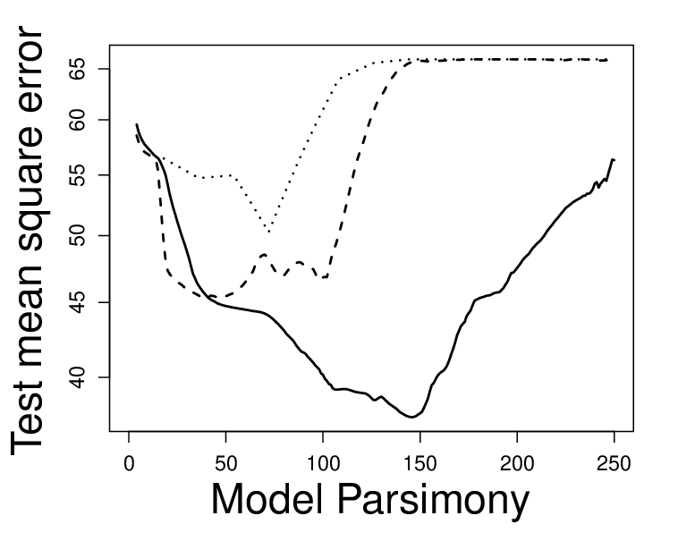
We compare our additive framework to (2) with fixed truncation, Kj=KK_{j}=K, in the low-dimensional setting and compare our sparse additive framework to that of Ravikumar et al. (2009), lasso (Tibshirani, 1996), and elastic net (Zou & Hastie, 2005) in the high-dimensional setting. For computational convenience, we fit our proposal with conservative basis truncation (9) with K~=⌈(2​n/3)1/2⌉\tilde{K}=\lceil(2n/3)^{1/2}\rceil, the square-root of the number of training observations. In both settings, we fit our proposal with order m=3m=3. We fit Ravikumar et al.’s proposal with K=2,4,8K=2,4,8; for a fairer comparison, we use a polynomial basis expansion. Other values of KK, had comparable or worse performance and are not presented here. For each proposal, we also implement a relaxed version; re-fitting the selected non-zero coefficients via least squares. For a sequence of λ\lambda values, or sequence of KK for (2), we calculate the mean square test error and the model parsimony, the number of total non-zero basis functions used. Lower values of model parsimony correspond to more sparsity in either the number of components or truncation levels KjK_{j}. Figure 5, shows that our proposal outperforms competitors in the low and high-dimensional setting in terms of mean square error for a sequence of fitted models. The relaxed version of Ravikumar et al.’s method achieves a lower test error but at the cost of reduced parsimony. The linear models, implemented by lasso and elastic net, had a substantially higher test error compared to additive models.
Refer to caption
Refer to caption
Refer to caption
Figure 5: Analysis of Parkinson’s telemonitoring dataset. Left: Low-dimensional results for our proposal (Refer to caption), the simple truncation estimator (2) (Refer to caption) and our relaxed proposal (Refer to caption). Middle: High-dimensional results for our proposal (Refer to caption), Ravikumar et al.’s proposal with 2 (Refer to caption), 4 (Refer to caption), and 8 (Refer to caption) basis functions, lasso (Refer to caption) and elastic net (Refer to caption). Right: Results for the relaxed versions of all methods in the middle panel.

Acknowledgement

We thank the associate editor and two referees for insightful comments that improved the manuscript. This work was partially supported by National Institutes of Health grants to A.S. and N.S., and National Science Foundation grants to A.S.

Supplementary material

The online supplementary material (appended below) includes additional figures, algorithm details, extension to binary response, and proofs for results in Section 4. The R package HierBasis, available on https://github.com/asadharis/HierBasis, implements the proposed methods.

References

  • Arnold & Tibshirani (2014) Arnold, T. B. & Tibshirani, R. J. (2014). genlasso: Path algorithm for generalized lasso problems. R package version 1.3.
  • Candes et al. (2008) Candes, E. J., Wakin, M. B. & Boyd, S. P. (2008). Enhancing sparsity by reweighted ℓ1\ell_{1} minimization. Journal of Fourier analysis and applications 14, 877–905.
  • Čencov (1962) Čencov, N. (1962). Evaluation of an unknown distribution density from observations. Doklady 3, 1559–1562.
  • Chatterjee (2013) Chatterjee, S. (2013). Assumptionless consistency of the lasso. arXiv preprint arXiv:1303.5817 .
  • Combettes & Pesquet (2011) Combettes, P. L. & Pesquet, J. (2011). Proximal splitting methods in signal processing. In Fixed-Point Algorithms for Inverse Problems in Science and Engineering, H. H. Bauschke, R. S. Burachik, P. L. Combettes, V. Elser, D. R. Luke & H. Wolkowicz, eds. Springer New York, pp. 185–212.
  • Dumer (2006) Dumer, I. (2006). Covering an ellipsoid with equal balls. Journal of Combinatorial Theory, Series A 113, 1667–1676.
  • Friedman et al. (2010) Friedman, J. H., Hastie, T. J. & Tibshirani, R. J. (2010). Regularization paths for generalized linear models via coordinate descent. Journal of Statistical Software 33, 1–22.
  • Haris et al. (2016) Haris, A., Witten, D. & Simon, N. (2016). Convex modeling of interactions with strong heredity. Journal of Computational and Graphical Statistics 25, 981–1004.
  • Hastie et al. (2009) Hastie, T. J., Tibshirani, R. J. & Friedman, J. H. (2009). The Elements of Statistical Learning. Springer New York, 2nd ed.
  • Jenatton et al. (2010) Jenatton, R., Mairal, J., Bach, F. R. & Obozinski, G. R. (2010). Proximal methods for sparse hierarchical dictionary learning. In Proceedings of the 27th International Conference on Machine Learning (ICML-10).
  • Kim et al. (2009) Kim, S., Koh, K., Boyd, S. & Gorinevsky, D. (2009). ℓ1\ell_{1} trend filtering. SIAM Review 51, 339–360.
  • Koltchinskii & Yuan (2010) Koltchinskii, V. & Yuan, M. (2010). Sparsity in multiple kernel learning. Ann. Statist. 38, 3660–3695.
  • Lou et al. (2016) Lou, Y., Bien, J., Caruana, R. & Gehrke, J. (2016). Sparse partially linear additive models. Journal of Computational and Graphical Statistics 25, 1126–1140.
  • Mammen & van de Geer (1997) Mammen, E. & van de Geer, S. (1997). Locally adaptive regression splines. The Annals of Statistics 25, 387–413.
  • Meier et al. (2009) Meier, L., van de Geer, S. & Bühlmann, P. (2009). High-dimensional additive modeling. The Annals of Statistics 37, 3779–3821.
  • Meinshausen (2007) Meinshausen, N. (2007). Relaxed lasso. Computational Statistics & Data Analysis 52, 374–393.
  • Nadaraya (1964) Nadaraya, E. A. (1964). On estimating regression. Theory of Probability and Its Applications 9, 141–142.
  • Petersen et al. (2016) Petersen, A., Witten, D. & Simon, N. (2016). Fused lasso additive model. Journal of Computational and Graphical Statistics 25, 1005–1025.
  • Raskutti et al. (2012) Raskutti, G., Wainwright, M. J. & Yu, B. (2012). Minimax-optimal rates for sparse additive models over kernel classes via convex programming. The Journal of Machine Learning Research 13, 389–427.
  • Raskutti et al. (2009) Raskutti, G., Yu, B. & Wainwright, M. J. (2009). Lower bounds on minimax rates for nonparametric regression with additive sparsity and smoothness. In Advances in Neural Information Processing Systems.
  • Rauhut & Ward (2016) Rauhut, H. & Ward, R. (2016). Interpolation via weighted ℓ1\ell_{1} minimization. Applied and Computational Harmonic Analysis 40, 321 – 351.
  • Ravikumar et al. (2009) Ravikumar, P., Lafferty, J., Liu, H. & Wasserman, L. (2009). Sparse additive models. Journal of the Royal Statistical Society: Series B (Statistical Methodology) 71, 1009–1030.
  • Sadhanala & Tibshirani (2018) Sadhanala, V. & Tibshirani, R. J. (2018). Additive models with trend filtering. arXiv preprint arXiv:1702.05037 .
  • Stein (1981) Stein, C. M. (1981). Estimation of the mean of a multivariate normal distribution. The Annals of Statistics 9, 1135–1151.
  • Stone (1977) Stone, C. J. (1977). Consistent nonparametric regression. The Annals of Statistics 5, 595–620.
  • Tibshirani (1996) Tibshirani, R. J. (1996). Regression shrinkage and selection via the lasso. Journal of the Royal Statistical Society. Series B (Methodological) , 267–288.
  • Tibshirani (2014) Tibshirani, R. J. (2014). Adaptive piecewise polynomial estimation via trend filtering. The Annals of Statistics 42, 285–323.
  • Tsanas et al. (2010) Tsanas, A., Little, M. A., McSharry, P. E. & Ramig, L. O. (2010). Accurate telemonitoring of parkinson’s disease progression by noninvasive speech tests. IEEE transactions on Biomedical Engineering 57, 884–893.
  • van de Geer (2000) van de Geer, S. (2000). Empirical Processes in M-Estimation. Cambridge University Press.
  • van de Geer (2010) van de Geer, S. (2010). The Lasso with within group structure, vol. 7 of IMS Collections. Beachwood, Ohio, USA: Institute of Mathematical Statistics, pp. 235–244.
  • van de Geer & Bühlmann (2009) van de Geer, S. & Bühlmann, P. (2009). On the conditions used to prove oracle results for the lasso. Electronic Journal of Statistics 3, 1360–1392.
  • Wahba (1990) Wahba, G. (1990). Spline Models for Observational Data. SIAM.
  • Watson (1964) Watson, G. S. (1964). Smooth regression analysis. Sankhyā: The Indian Journal of Statistics, Series A 26, 359–372.
  • Yang & Barron (1999) Yang, Y. & Barron, A. (1999). Information-theoretic determination of minimax rates of convergence. The Annals of Statistics 27, 1564–1599.
  • Yuan & Lin (2006) Yuan, M. & Lin, Y. (2006). Model selection and estimation in regression with grouped variables. Journal of the Royal Statistical Society: Series B (Statistical Methodology) 68, 49–67.
  • Yuan & Zhou (2015) Yuan, M. & Zhou, D.-X. (2015). Minimax optimal rates of estimation in high dimensional additive models: Universal phase transition. arXiv preprint arXiv:1503.02817 .
  • Zhao et al. (2014) Zhao, T., Li, X., Liu, H. & Roeder, K. (2014). SAM: Sparse Additive Modelling. R package version 1.0.5.
  • Zou & Hastie (2005) Zou, H. & Hastie, T. J. (2005). Regularization and variable selection via the elastic net. Journal of the Royal Statistical Society: Series B (Statistical Methodology) 67, 301–320.

Appendix A Additional figures

In this appendix we present some additional figures referenced in Sections 2, 5 and 6 of the main manuscript.

Figure A.1, shows examples of some fitted models for a fixed value of degrees of freedom. Our method seems to perform very well and is mostly robust to changes in the value of mm. The smoothing splines estimates are unable to do as well for the same effective degrees of freedom. The plots in the bottom panel of Figure A.1 also suggest that first order trend filter can perform poorly in presence of model misspecification.

In Figure A.2, we show some of the fitted functions for both Ravikumar et al.’s method and our proposal using the λ\lambda value which minimizes the test set error for Ravikumar et al.’s proposal with 33 and 1010 basis functions.

In Figure A.3, we show examples of basis functions which possess a natural hierarchy. Our proposal is specifically suited for such systems of hierarchical basis functions.

Refer to caption
Refer to caption
Refer to caption
Refer to caption
Figure A.1: Top row: Scatter plots of one simulated data along with the true functions (Refer to caption). Second row: The first row figures with estimated functions for our proposal with m=1m=1 (Refer to caption), 22 (Refer to caption), and 3 (Refer to caption). Third row: The first row figures with estimated functions via smoothing splines (Refer to caption). Fourth row: The first row figures with estimated functions for trend filtering of order 1 (Refer to caption), 2 (Refer to caption), and 3 (Refer to caption).
Refer to caption
Figure A.2: The first 4 component functions of the simulation study from Section 5.2. We show the estimates of our proposal (Refer to caption), and that of Ravikumar et al. (2009) fitted with 10 (Refer to caption) and 3 (Refer to caption) basis functions. In each case, the tuning parameter leading to the smallest mean square error was used.
Refer to caption
Figure A.3: Examples of basis functions with natural hierarchical complexity; we plot ψ1​(x)\psi_{1}(x) (Refer to caption), ψ2​(x)\psi_{2}(x) (Refer to caption), ψ3​(x)\psi_{3}(x) (Refer to caption), ψ4​(x)\psi_{4}(x) (Refer to caption). Polynomial, trigonometric and wavelet basis functions are shown in the left, middle and right panels, respectively.

Appendix B Algorithms for additive framework and extension to classification

Here we give an algorithm for our additive and sparse additive framework as well as an algorithm for the extension of our proposal to classification. We use a block coordinate descent algorithm for solving the additive and sparse additive proposal. This algorithm cyclically iterates through features, and for each feature applies the univariate solution detailed in Algorithm 1 of the main manuscript. The exact details are given in Algorithm 2 below.

Initialize βj←0{\beta}_{j}\leftarrow 0 for j=1,…,pj=1,\ldots,p
While l≤m​a​x​_​i​t​e​rl\leq max\_iter and not converged
  For j=1,…,pj=1,\,\ldots,\,p       Set r−j←y−∑j′≠jΨK~j′βj′{r}_{-j}\leftarrow{y}-\sum_{j^{{}^{\prime}}\neq j}{\Psi}_{\tilde{K}}^{j^{{}^{\prime}}}{{\beta}}_{j^{{}^{\prime}}}       Update βj←arg⁡minβ∈ℝK~12‖r−j−ΨK~jβ‖n2+λ2∑k=1K~w~k‖Ψk:K~jβj,k:K~‖n,{\beta}_{j}\leftarrow\underset{{\beta}\in\mathbb{R}^{\tilde{K}}}{\arg\min}\frac{1}{2}\left\|{r}_{-j}-{\Psi}_{\tilde{K}}^{j}{\beta}\right\|_{n}^{2}+\lambda^{2}\sum_{k=1}^{\tilde{K}}\widetilde{w}_{k}\left\|{\Psi}^{j}_{k:\tilde{K}}{\beta}_{j,k:\tilde{K}}\right\|_{n},         where w~1=w1+λ−1\widetilde{w}_{1}=w_{1}+\lambda^{-1} and w~k=wk\widetilde{w}_{k}=w_{k} for k=2,…,K~k=2,\,\ldots,\,\tilde{K}.
 Return β1,…,βp{\beta}_{1},\,\ldots,\,{\beta}_{p}
Algorithm 2 Block coordinate descent for the additive and sparse additive framework

We also give an algorithm for the extension of our method to classification based on proximal gradient descent. To begin let L(β0,β)=1/(2n)∑i=1nlog(1+exp[−yi{β0+(Ψβ)i}])L(\beta_{0},{\beta})={1}/({2n})\sum_{i=1}^{n}\log\left(1+\exp\left[-y_{i}\left\{\beta_{0}+\left(\Psi{\beta}\right)_{i}\right\}\right]\right). We denote by ∇L​(β0,β)\nabla L(\beta_{0},{\beta}), the derivative of LL at the point (β0,β)∈ℝK~+1(\beta_{0},\,{\beta})\in\mathbb{R}^{\tilde{K}+1}. Algorithm 3 presents the steps for solving (13). The algorithm for extension of additive models to classification can be similarly derived and is omitted in the interest of brevity.

 Initialize (β00,β0)(\beta_{0}^{0},{\beta}^{0})
 For l=1, 2,…l=1,\,2,\,\ldots until convergence
  Select a step size tlt_{l} via line search
  Update
(β0l,βl)←arg⁡min(β0,β)∈ℝK~+112‖(β0,β)−{(β0l−1,βl−1)−tl∇L(β0l−1,βl−1)}‖22+λΩ(β).(\beta_{0}^{l},\,{\beta}^{l})\leftarrow\underset{(\beta_{0},{\beta})\in\mathbb{R}^{\tilde{K}+1}}{\arg\min}\frac{1}{2}\left\|(\beta_{0},{\beta})-\left\{(\beta_{0}^{l-1},{\beta}^{l-1})-t_{l}\nabla L(\beta_{0}^{l-1},{\beta}^{l-1})\right\}\right\|^{2}_{2}+\lambda\Omega({\beta}).
 Return (β0l,βl)(\beta_{0}^{l},{\beta}^{l})
Algorithm 3 Proximal gradient descent for extension to classification

Appendix C Proofs for Section 4.3

of Lemma 2.

Firstly, we have for fβ[1]​(x)=∑k=1K~nψ⁡(x)​βk[1],fβ[2]​(x)=∑k=1K~nψ⁡(x)​βk[2]∈ℱnf_{\beta^{[1]}}(x)=\sum_{k=1}^{\tilde{K}_{n}}\psi(x)\beta_{k}^{[1]},\,f_{\beta^{[2]}}(x)=\sum_{k=1}^{\tilde{K}_{n}}\psi(x)\beta_{k}^{[2]}\in\mathcal{F}_{n}

‖fβ[1]−fβ[1]‖Q2\displaystyle\|f_{\beta^{[1]}}-f_{\beta^{[1]}}\|_{Q}^{2} =∫(fβ[1]−fβ[1])2​𝑑Q=∫{∑k=1K~nψk​(x)​(βk[1]−βk[2])}2​𝑑Q\displaystyle=\int(f_{\beta^{[1]}}-f_{\beta^{[1]}})^{2}dQ=\int\left\{\sum_{k=1}^{\tilde{K}_{n}}\psi_{k}(x)(\beta^{[1]}_{k}-\beta^{[2]}_{k})\right\}^{2}dQ
=∫{∑k=1K~nψk2​(x)​(βk[1]−βk[2])2+∑k≠lψk​(x)​ψl​(x)​(βk[1]−βk[2])​(βl[1]−βl[2])}​𝑑Q\displaystyle=\int\left\{\sum_{k=1}^{\tilde{K}_{n}}\psi_{k}^{2}(x)\left(\beta^{[1]}_{k}-\beta^{[2]}_{k}\right)^{2}+\sum_{k\not=l}\psi_{k}(x)\psi_{l}(x)\left(\beta^{[1]}_{k}-\beta^{[2]}_{k}\right)\left(\beta^{[1]}_{l}-\beta^{[2]}_{l}\right)\right\}dQ
=‖β[1]−β[2]‖22,\displaystyle=\left\|\beta^{[1]}-\beta^{[2]}\right\|_{2}^{2},

where the final equality follows due to the orthonormality of ψk\psi_{k}. Similarly for fβ[1],fβ[1]∈ℱp,nf_{\beta^{[1]}},f_{\beta^{[1]}}\in\mathcal{F}_{p,n} we can show that ‖fβ[1]−fβ[1]‖Q2=‖β[1]−β[2]‖22\|f_{\beta^{[1]}}-f_{\beta^{[1]}}\|_{Q}^{2}=\|{\beta}^{[1]}-{\beta}^{[2]}\|_{2}^{2}. Thus if {β1,…,βN}\{{\beta}^{1},\ldots,{\beta}^{N}\} is the smallest δ\delta-cover of HK~nw/MH^{w/M}_{\tilde{K}_{n}} then the functions {fβ1,…,fβN}\{f_{\beta^{1}},\ldots,f_{\beta^{N}}\} form the smallest δ\delta-cover with respect to the LQL_{Q} norm. This can be extended to the case n=∞n=\infty. This proves the first part.

Secondly, note that for fβ[1],fβ[2]∈ℱnf_{\beta^{[1]}},f_{\beta^{[2]}}\in\mathcal{F}_{n}

‖fβ[1]−fβ[2]‖n2=(β[1]−β[2])⊤​ΨK~n⊤​ΨK~nn​(β[1]−β[2])≤Λmax​‖β[1]−β[2]‖22,\|f_{\beta^{[1]}}-f_{\beta^{[2]}}\|_{n}^{2}=({\beta}^{[1]}-{\beta}^{[2]})^{\top}\frac{{\Psi}_{\tilde{K}_{n}}^{\top}{\Psi}_{\tilde{K}_{n}}}{n}({\beta}^{[1]}-{\beta}^{[2]})\leq\Lambda_{\max}\|{\beta}^{[1]}-{\beta}^{[2]}\|_{2}^{2},

thus if {β1,…,βN}\{{\beta}^{1},\ldots,{\beta}^{N}\} is the smallest δ\delta-cover for ℋK~nw\mathcal{H}_{\tilde{K}_{n}}^{w}, then {fβ1,…,fβN}\{f_{\beta^{1}},\ldots,f_{\beta^{N}}\} is a Λmax1/2​δ\Lambda_{\max}^{1/2}\delta cover of {fβ∈ℱn:∑k=1K~nwk∥Ψk:K~nβk:K~n∥≤1}\{f_{\beta}\in\mathcal{F}_{n}:\sum_{k=1}^{\tilde{K}_{n}}w_{k}\|{\Psi}_{k:\tilde{K}_{n}}{\beta}_{k:\tilde{K}_{n}}\|\leq 1\} with respect to the QnQ_{n} metric. Since this is a cover and not the smallest cover, we have

H[Λmax1/2δ,{fβ∈ℱn:∑k=1K~nwk∥Ψk:K~nβk:K~n∥≤1},Qn]≤H(δ,ℋK~nw),H\Big[\Lambda_{\max}^{1/2}\delta,\{f_{\beta}\in\mathcal{F}_{n}:\sum_{k=1}^{\tilde{K}_{n}}w_{k}\|{\Psi}_{k:\tilde{K}_{n}}{\beta}_{k:\tilde{K}_{n}}\|\leq 1\},Q_{n}\Big]\leq H(\delta,\mathcal{H}_{\tilde{K}_{n}}^{w}),

and since the inequality holds for all δ>0\delta>0, we can select δ=δ′Λmax−1/2\delta=\delta^{\prime}\Lambda_{\max}^{-1/2} giving us the result.

For the multivariate case we can repeat the same argument as above replacing ℱn\mathcal{F}_{n} by ℱp,n\mathcal{F}_{p,n}. ∎

of Lemma 3.

For the Ellipsoid EK~nwE_{\tilde{K}_{n}}^{w} where

EK~nw={β∈ℝK~n:∑k=1K~nβk2​(w1+⋯+wk)2≤1},E^{w}_{\tilde{K}_{n}}=\left\{{\beta}\in\mathbb{R}^{\tilde{K}_{n}}:\sum_{k=1}^{\tilde{K}_{n}}\beta_{k}^{2}\left(w_{1}+\cdots+w_{k}\right)^{2}\leq 1\right\}\ , (C.1)

we show that ℋK~nw⊂EK~nw\mathcal{H}_{\tilde{K}_{n}}^{w}\subset E_{\tilde{K}_{n}}^{w} in Lemma F8 of Appendix F. Dumer (2006) proved an upper bound for ellipsoids which we state in Appendix G.1. For the special case of wk=km−(k−1)mw_{k}=k^{m}-(k-1)^{m}, this theorem yields the desired upper bound as shown in Corollary G1. Therefore we have H(δ,ℋK~nw)≤H(δ,EK~nw)≤UE,1δ−1/mH(\delta,\,\mathcal{H}_{\tilde{K}_{n}}^{w})\leq H(\delta,\,E_{\tilde{K}_{n}}^{w})\leq U_{E,1}\delta^{-{1}/{m}}.

Similarly, we can consider the special case of our multivariate framework weights in Corollary G2, which gives us the result H(δ,ℋK~nw)≤H(δ,EK~nw)≤UE,2δ−p/mH(\delta,\,\mathcal{H}_{\tilde{K}_{n}}^{w})\leq H(\delta,\,E_{\tilde{K}_{n}}^{w})\leq U_{E,2}\delta^{-{p}/{m}}. ∎

of Lemma 4.

Let dd be the integer such that (w1+⋯+wd+1)−1≤δ≤(w1+⋯+wd)−1(w_{1}+\cdots+w_{d+1})^{-1}\leq\delta\leq(w_{1}+\cdots+w_{d})^{-1} for δ∈((w1+⋯+wK~n+1)−1,1)\delta\in((w_{1}+\cdots+w_{\tilde{K}_{n}+1})^{-1},1). Note that since δ≥(w1+⋯+wK~n+1)−1\delta\geq(w_{1}+\cdots+w_{\tilde{K}_{n}+1})^{-1}, d≤K~nd\leq\tilde{K}_{n}. We define the truncated region as

H~dw={β∈ℋK~nw:βj=0​ for all ​j≥d+1}.\widetilde{H}_{d}^{w}=\left\{{\beta}\in\mathcal{H}_{\tilde{K}_{n}}^{w}:\beta_{j}=0\ \text{ for all }\ j\geq d+1\right\}.

Then we have that ℋdw⊂ℋ~dw⊆ℋK~nw\mathcal{H}_{d}^{w}\subset\widetilde{\mathcal{H}}_{d}^{w}\subseteq\mathcal{H}_{\tilde{K}_{n}}^{w} where ℋdw\mathcal{H}_{d}^{w} is simply viewing ℋ~dw\widetilde{\mathcal{H}}_{d}^{w} as a subset of ℝd\mathbb{R}^{d}. Let 𝔹n​(r)\mathbb{B}_{n}(r) be the nn-ball of radius rr. By Lemma F9, we have 𝔹d​{(w1+⋯+wd)−1}⊂ℋdw\mathbb{B}_{d}\left\{(w_{1}+\cdots+w_{d})^{-1}\right\}\subset\mathcal{H}_{d}^{w}. The lower bound of the entropy of a ball can be obtained by a simple volume argument. Since (w1+⋯+wd)−1≥δ(w_{1}+\cdots+w_{d})^{-1}\geq\delta then 𝔹d​(δ)⊆𝔹d​{(w1+⋯+wd)−1}\mathbb{B}_{d}(\delta)\subseteq\mathbb{B}_{d}\{(w_{1}+\cdots+w_{d})^{-1}\} and hence

H⁡(δ/2,ℋdw)≥H⁡{δ/2,𝔹d​(δ)}≥log⁡V​o​l​{𝔹d​(δ)}V​o​l​{𝔹d​(δ/2)}=d​log⁡(2).\displaystyle H(\delta/2,\mathcal{H}_{d}^{w})\geq H\{\delta/2,\mathbb{B}_{d}\left(\delta\right)\}\geq\log\frac{Vol\{\mathbb{B}_{d}\left(\delta\right)\}}{Vol\{\mathbb{B}_{d}(\delta/2)\}}=d\log(2).

Since the above inequality holds for δ≤1\delta\leq 1, for δ∈((w1+⋯+wK~n+1)−1, 1/2)\delta\in((w_{1}+\cdots+w_{\tilde{K}_{n}+1})^{-1},\,1/2) we have H⁡(δ,ℋdw)≥d​log⁡2H(\delta,\mathcal{H}_{d}^{w})\geq d\log 2.

Now for the univariate case we have (w1+⋯+wd+1)−1=(d+1)−m≤δ(w_{1}+\cdots+w_{d+1})^{-1}=(d+1)^{-m}\leq\delta or (d+1)≥δ−1/m(d+1)\geq\delta^{-{1}/{m}} and hence we have

H(δ,ℋdw)≥dlog2≥(δ−1/m−1)log2=δ−1/m(1−δ1/m)log2≥δ−1/m(1−2−1/m)log2.\displaystyle H(\delta,\mathcal{H}_{d}^{w})\geq d\log 2\geq(\delta^{-{1}/{m}}-1)\log 2=\delta^{-{1}/{m}}\left(1-\delta^{1/m}\right)\log 2\geq\delta^{-{1}/{m}}\left(1-2^{-1/m}\right)\log 2.

Now for the multivariate case, the argument is slightly different due to presence of zero weights. As before, there is some d′d^{\prime} such that (w1+⋯+wqd′−1)−1≤δ≤(w1+⋯+wqd′)−1(w_{1}+\cdots+w_{q_{d^{\prime}}-1})^{-1}\leq\delta\leq(w_{1}+\cdots+w_{q_{d^{\prime}}})^{-1} and hence d=qd′−1d=q_{d^{\prime}}-1. Note that by assumption we have K~n=qK~′−1\tilde{K}_{n}=q_{\tilde{K}^{\prime}}-1 and hence δ≥(w1+⋯+wqK~′)−1\delta\geq(w_{1}+\cdots+w_{q_{\tilde{K}^{\prime}}})^{-1} which implies that d′≤K~′d^{\prime}\leq\tilde{K}^{\prime} and hence d≤K~nd\leq\tilde{K}_{n}. Finally we have that since w1+⋯+wqd′−1=w1+⋯+wqd′−1=(d′−1)mw_{1}+\cdots+w_{q_{d^{\prime}}-1}=w_{1}+\cdots+w_{q_{d^{\prime}-1}}=(d^{\prime}-1)^{m}, therefore d′−1≥δ−1/md^{\prime}-1\geq\delta^{-{1}/{m}}. Now we have that

H⁡(δ,ℋdw)\displaystyle H(\delta,\mathcal{H}_{d}^{w}) ≥d​log⁡(2)=(qd′−1)​log⁡(2)={(d′+p−1p)−1}​log⁡(2)\displaystyle\geq d\log(2)=(q_{d^{\prime}}-1)\log(2)=\left\{\binom{d^{\prime}+p-1}{p}-1\right\}\log(2)
≥{(d′+p−1)ppp−1}​log⁡(2)≥{(δ−1/m+p)ppp−1}​log⁡(2)\displaystyle\geq\left\{\frac{(d^{\prime}+p-1)^{p}}{p^{p}}-1\right\}\log(2)\geq\left\{\frac{(\delta^{-{1}/{m}}+p)^{p}}{p^{p}}-1\right\}\log(2)
=δ−p/m{(1+p​δ1/m)ppp−δp/m}⏟g⁡(δ)log(2)≥δ−p/mAlog(2),\displaystyle=\delta^{-{p}/{m}}\underbrace{\left\{\frac{(1+p\delta^{1/m})^{p}}{p^{p}}-\delta^{{p}/{m}}\right\}}_{g(\delta)}\log(2)\geq\delta^{-{p}/{m}}A\log(2),

where the last inequality follows from the fact that g′​(δ)>0g^{\prime}(\delta)>0 for all δ∈(0,1)\delta\in(0,1). ∎

Appendix D Details for Proposition 2

D.1 Univariate case

Firstly, if f0​(x)=∑k=1∞ψk​(x)​βk0f^{0}(x)=\sum_{k=1}^{\infty}\psi_{k}(x)\beta^{0}_{k} then we select fn∗​(x)=∑k=1K~nψk​(x)​βk0∈ℱnf_{n}^{*}(x)=\sum_{k=1}^{\tilde{K}_{n}}\psi_{k}(x)\beta^{0}_{k}\in\mathcal{F}_{n}. Secondly, we note that for the univariate estimator we have Ω(fn∗∣Qn)=Ωuni(β1:K~n0)\Omega(f_{n}^{*}\mid Q_{n})=\Omega^{\text{uni}}({\beta}^{0}_{1:\tilde{K}_{n}}). For brevity we will drop the dependence on β0{\beta}^{0} and denote Ωuni(β1:K~n0)\Omega^{\text{uni}}({\beta}^{0}_{1:\tilde{K}_{n}}) by Ω\Omega. Thus we have

λn2​Ω​(fn∗∣Qn)\displaystyle\lambda_{n}^{2}\Omega(f_{n}^{*}\mid Q_{n}) =n−2/(2+α)Ω−(2−α)/(2+α)Ω=n−2/(2+α)Ω2​α/(2+α)=n−2m/(2m+1)Ω2/(2​m+1),\displaystyle=n^{-{2}/{(2+\alpha)}}\Omega^{-{(2-\alpha)}/{(2+\alpha)}}\Omega=n^{-{2}/{(2+\alpha)}}\Omega^{{2\alpha}/{(2+\alpha)}}=n^{-{2m}/{(2m+1)}}\Omega^{{2}/{(2m+1)}},

where we use the fact that for our class α=1/m\alpha=1/m. For the term Ω(β1:K~n0)\Omega({\beta}^{0}_{1:\tilde{K}_{n}}) we have

Ω(β1:K~n0)\displaystyle\Omega({\beta}^{0}_{1:\tilde{K}_{n}}) =∑k=1K~nwk{(β1:K~n0)⊤Ψk:K~n⊤Ψk:K~nnβ1:K~n0}1/2≤Λmax1/2∑k=1K~nwk∥β1:K~n0∥2≤Λmax1/2M,\displaystyle=\sum_{k=1}^{\tilde{K}_{n}}w_{k}\Big\{\left({\beta}^{0}_{1:\tilde{K}_{n}}\right)^{\top}\frac{{\Psi}_{k:\tilde{K}_{n}}^{\top}{\Psi}_{k:\tilde{K}_{n}}}{n}{\beta}^{0}_{1:\tilde{K}_{n}}\Big\}^{1/2}\leq\Lambda^{1/2}_{\max}\sum_{k=1}^{\tilde{K}_{n}}w_{k}\|{\beta}^{0}_{1:\tilde{K}_{n}}\|_{2}\leq\Lambda^{1/2}_{\max}M,

for f0∈ℱ∞Mf^{0}\in\mathcal{F}_{\infty}^{M}. For 𝒢2M\mathcal{G}_{2}^{M}, we do not have the above bound and hence we keep the Ω\Omega term in the inequality.

For the truncation error we note that

‖f0−fn∗‖n2\displaystyle\|f^{0}-f_{n}^{*}\|_{n}^{2} =1n​∑i=1n{∑k=K~n+1∞ψk​(xi)​βk0}2\displaystyle=\frac{1}{n}\sum_{i=1}^{n}\left\{\sum_{k=\tilde{K}_{n}+1}^{\infty}\psi_{k}(x_{i})\beta^{0}_{k}\right\}^{2}
≤ψmax2​1n​∑i=1n(∑k=K~n+1∞βk0)2=ψmax2​(∑k=K~n+1∞βk0)2\displaystyle\leq\psi_{\max}^{2}\frac{1}{n}\sum_{i=1}^{n}\left(\sum_{k=\tilde{K}_{n}+1}^{\infty}\beta^{0}_{k}\right)^{2}=\psi_{\max}^{2}\left(\sum_{k=\tilde{K}_{n}+1}^{\infty}\beta_{k}^{0}\right)^{2}
=ψmax2​(∑k=K~n+1∞kmkm​|βk0|)2\displaystyle=\psi_{\max}^{2}\left(\sum_{k=\tilde{K}_{n}+1}^{\infty}\frac{k^{m}}{k^{m}}|\beta^{0}_{k}|\right)^{2}
≤ψmax2​{∑k=K~n+1∞k2​m​(βk0)2}​(∑k=K~n+1∞1k2​m),\displaystyle\leq\psi_{\max}^{2}\left\{\sum_{k=\tilde{K}_{n}+1}^{\infty}k^{2m}(\beta^{0}_{k})^{2}\right\}\left(\sum_{k=\tilde{K}_{n}+1}^{\infty}\frac{1}{k^{2m}}\right),
≤=ψmax2M2∑k=K~n+1∞k−2​m,\displaystyle\leq=\psi_{\max}^{2}M^{2}\sum_{k=\tilde{K}_{n}+1}^{\infty}{k^{-2m}},

where the last inequality follows from the proof of Lemma F8. The result now follows since

∑k=K~n+1∞k−2​m≤{(2​m−1)​(K~n+1)2​m−1}−1≤12​m−1​1K~n2​m−1.\displaystyle\sum_{k=\tilde{K}_{n}+1}^{\infty}k^{-2m}\leq\left\{(2m-1)(\tilde{K}_{n}+1)^{2m-1}\right\}^{-1}\leq\frac{1}{2m-1}\frac{1}{\tilde{K}_{n}^{2m-1}}.

D.2 Multivariate case

Now we assume that f0​(x)=∑k=1∞ψk​(xνk)​βk0f^{0}({x})=\sum_{k=1}^{\infty}\psi_{k}({x}^{{\nu_{k}}})\beta^{0}_{k} for x∈ℝp{x}\in\mathbb{R}^{p} and νk∈ℤ+p\nu_{k}\in\mathbb{Z}_{+}^{p}. Then we take fn∗​(x)=∑k=1K~nψk​(xνk)​βk0f_{n}^{*}({x})=\sum_{k=1}^{\tilde{K}_{n}}\psi_{k}({x}^{{\nu_{k}}})\beta^{0}_{k}. Now by the same calculations as in the univariate case, we have

λn2​Ω​(fn∗∣Qn)\displaystyle\lambda_{n}^{2}\Omega(f_{n}^{*}\mid Q_{n}) =n−2m/(2m+p)Ω2​p/(2​m+p)≤n−2m/(2m+p)(Λmax1/2M)2​p/(2​m+p).\displaystyle=n^{-{2m}/{(2m+p)}}\Omega^{{2p}/{(2m+p)}}\leq n^{-{2m}/{(2m+p)}}({\Lambda^{1/2}_{\max}}M)^{{2p}/{(2m+p)}}.

For the truncation error we note that K~n=qK~′−1\tilde{K}_{n}=q_{\tilde{K}^{\prime}}-1 and hence

‖f0−fn∗‖n2\displaystyle\|f^{0}-f_{n}^{*}\|_{n}^{2} =1n​∑i=1n{∑k=K~n+1∞ψk​(xiνk)​βk0}2≤ψmax2​1n​∑i=1n(∑k=qK~′∞βk0)2\displaystyle=\frac{1}{n}\sum_{i=1}^{n}\left\{\sum_{k=\tilde{K}_{n}+1}^{\infty}\psi_{k}({x_{i}}^{{\nu_{k}}})\beta^{0}_{k}\right\}^{2}\leq\psi_{\max}^{2}\frac{1}{n}\sum_{i=1}^{n}\left(\sum_{k=q_{\tilde{K}^{\prime}}}^{\infty}\beta^{0}_{k}\right)^{2}
=ψmax21n∑i=1n{∑k:‖νk‖1=K~′K~′mK~′m|βk0|+∑k:‖νk‖1=K~′+1(K~′+1)m(K~′+1)m|βk0|+⋯}2\displaystyle=\psi_{\max}^{2}\frac{1}{n}\sum_{i=1}^{n}\left\{\sum_{k:\|{\nu_{k}}\|_{1}=\tilde{K}^{\prime}}\frac{\tilde{K}^{\prime m}}{\tilde{K}^{\prime m}}|\beta^{0}_{k}|+\sum_{k:\|{\nu_{k}}\|_{1}=\tilde{K}^{\prime}+1}\frac{(\tilde{K}^{\prime}+1)^{m}}{(\tilde{K}^{\prime}+1)^{m}}|\beta^{0}_{k}|+\cdots\right\}^{2}
=ψmax21n∑i=1n(∑R=K~′∞RmRm∑k:‖νk‖1=R|βk0|)2\displaystyle=\psi_{\max}^{2}\frac{1}{n}\sum_{i=1}^{n}\left(\sum_{R=\tilde{K}^{\prime}}^{\infty}\frac{R^{m}}{R^{m}}\sum_{k:\|{\nu_{k}}\|_{1}=R}|\beta^{0}_{k}|\right)^{2}
=ψmax21n∑i=1n{(∑R=K~′∞1R2​m)1/2(∑R=K′∞Rm∑k:‖νk‖1=R|βk0|)1/2}2\displaystyle=\psi_{\max}^{2}\frac{1}{n}\sum_{i=1}^{n}\left\{\left(\sum_{R=\tilde{K}^{\prime}}^{\infty}\frac{1}{R^{2m}}\right)^{1/2}\left(\sum_{R=K^{\prime}}^{\infty}R^{m}\sum_{k:\|{\nu_{k}}\|_{1}=R}|\beta^{0}_{k}|\right)^{1/2}\right\}^{2}
≤ψmax2​M2​∑R=K~′∞1R2​m≤M2​ψmax22​m−1​1(K~′)2​m−1.\displaystyle\leq\psi_{\max}^{2}M^{2}\sum_{R=\tilde{K}^{\prime}}^{\infty}\frac{1}{R^{2m}}\leq\frac{M^{2}\psi_{\max}^{2}}{2m-1}\frac{1}{(\tilde{K}^{\prime})^{2m-1}}.

Appendix E Proof of Theorem 4

E.1 Initial results

Recall that (f^j)j=1p∈ℱ(\widehat{f}_{j})_{j=1}^{p}\in\mathcal{F} where ℱ\mathcal{F} is some arbitrary univariate function class . We denote the functions f^​(x)=∑j=1pf^j​(xj)\widehat{f}({x})=\sum_{j=1}^{p}\widehat{f}_{j}({x}_{j}) and f0​(x)=∑j=1pfj0​(xj)f^{0}({x})=\sum_{j=1}^{p}f^{0}_{j}({x}_{j}) for x=(x1,…,xp)⊤∈ℝp{x}=(x_{1},\ldots,x_{p})^{\top}\in\mathbb{R}^{p}. For the proof of Theorem 4, λn\lambda_{n} and ρn\rho_{n} are functions of nn but for convenience we will simply write λ,ρ\lambda,\,\rho. Throughout this proof, instead of the smoothness level mm, we will use α=1/m\alpha=1/m. Thus the entropy condition is H⁡[δ,{f∈ℱ:Ω⁡(f)≤1},Qn]≤A0​δ−α,H[\delta,\{f\in\mathcal{F}:\Omega(f)\leq 1\},Q_{n}]\leq A_{0}\delta^{-\alpha}, for α∈(0,2)\alpha\in(0,2), and so forth.

We begin the proof of Theorem 4 with a basic inequality.

Lemma 5 (Basic inequality).

For any function f∗=∑j=1pfj∗f^{*}=\sum_{j=1}^{p}f_{j}^{*}, where fj∗∈ℱf_{j}^{*}\in\mathcal{F} and, the solution f^\widehat{f} of (17), we have the following basic inequality

12​‖f^−f0‖n2+λ​Ip​(f^)≤|⟨ε,f^−f∗⟩n|+λ​Ip​(f∗)+|ε¯|​∑j=1p‖f^j−fj∗‖n+12​‖f∗−f0‖n2,\frac{1}{2}\|\widehat{f}-f^{0}\|_{n}^{2}+\lambda I_{p}(\widehat{f})\leq|\langle\varepsilon,\,\widehat{f}-f^{*}\rangle_{n}|+\lambda I_{p}(f^{*})+|\bar{\varepsilon}|\sum_{j=1}^{p}\|\widehat{f}_{j}-f^{*}_{j}\|_{n}+\frac{1}{2}\|f^{*}-f^{0}\|_{n}^{2},

where ⟨ε,f⟩n=n−1​∑i=1nεi​f​(xi)\langle\varepsilon,f\rangle_{n}={n}^{-1}\sum_{i=1}^{n}\varepsilon_{i}f({x_{i}}), ε¯=n−1​∑i=1nεi\bar{\varepsilon}={n}^{-1}\sum_{i=1}^{n}\varepsilon_{i} and Ip​(f)=∑j=1pI⁡(fj)=∑j=1p‖fj‖n+λ​Ω​(fj)I_{p}(f)=\sum_{j=1}^{p}I(f_{j})=\sum_{j=1}^{p}\|f_{j}\|_{n}+\lambda\Omega(f_{j}) for an additive function ff.

Proof.

We have

12​n​∑i=1n{yi−y¯−f^​(xi)}2+λ​Ip​(f^)≤12​n​∑i=1n{yi−y¯−f∗​(xi)}2+λ​Ip​(fj∗),\displaystyle\frac{1}{2n}\sum_{i=1}^{n}\left\{y_{i}-\bar{y}-\widehat{f}({x_{i}})\right\}^{2}+\lambda I_{p}(\widehat{f})\leq\frac{1}{2n}\sum_{i=1}^{n}\left\{y_{i}-\bar{y}-f^{*}({x_{i}})\right\}^{2}+\lambda I_{p}(f^{*}_{j}),

which is equivalent to

12​n​∑i=1n{εi+c0−y¯−(f^−f0)​(xi)}2+λ​Ip​(f^)≤12​n​∑i=1n{εi+c0−y¯−(f∗−f0)​(xi)}2+λ​Ip​(fj∗).\displaystyle\frac{1}{2n}\sum_{i=1}^{n}\left\{\varepsilon_{i}+c^{0}-\bar{y}-(\widehat{f}-f^{0})({x_{i}})\right\}^{2}+\lambda I_{p}(\widehat{f})\leq\frac{1}{2n}\sum_{i=1}^{n}\left\{\varepsilon_{i}+c^{0}-\bar{y}-(f^{*}-f^{0})({x_{i}})\right\}^{2}+\lambda I_{p}(f^{*}_{j}).

This gives us

12​n​∑i=1n(εi+c0−y¯)2+(f^−f0)2​(xi)−2​(εi+c0−y¯)​(f^−f0)​(xi)+λ​Ip​(f^)\displaystyle\frac{1}{2n}\sum_{i=1}^{n}\left(\varepsilon_{i}+c^{0}-\bar{y}\right)^{2}+(\widehat{f}-f^{0})^{2}({x_{i}})-2(\varepsilon_{i}+c^{0}-\bar{y})(\widehat{f}-f^{0})({x_{i}})+\lambda I_{p}(\widehat{f})
≤12​n​∑i=1n(εi+c0−y¯)2+(f∗−f0)2​(xi)−2​(εi+c0−y¯)​(f∗−f0)​(xi)+λ​Ip​(f∗).\displaystyle\leq\frac{1}{2n}\sum_{i=1}^{n}\left(\varepsilon_{i}+c^{0}-\bar{y}\right)^{2}+(f^{*}-f^{0})^{2}({x_{i}})-2(\varepsilon_{i}+c^{0}-\bar{y})(f^{*}-f^{0})({x_{i}})+\lambda I_{p}(f^{*}).

Re-arranging the terms and simplifying gives us

12​‖f^−f0‖n2−⟨ε+c0−y¯,f^−f0⟩n+λ​Ip​(f^)\displaystyle\frac{1}{2}\|\widehat{f}-f^{0}\|_{n}^{2}-\langle\varepsilon+c^{0}-\bar{y},\,\widehat{f}-f^{0}\rangle_{n}+\lambda I_{p}(\widehat{f})
≤12​‖f∗−f0‖n2−⟨ε+c0−y¯,f∗−f^⟩n−⟨ε+c0−y¯,f^−f0⟩n+λ​Ip​(f∗),\displaystyle\leq\frac{1}{2}\|f^{*}-f^{0}\|_{n}^{2}-\langle\varepsilon+c^{0}-\bar{y},\,f^{*}-\widehat{f}\rangle_{n}-\langle\varepsilon+c^{0}-\bar{y},\,\widehat{f}-f^{0}\rangle_{n}+\lambda I_{p}(f^{*}),

which implies

12​‖f^−f0‖n2+λ​Ip​(f^)≤12​‖f∗−f0‖n2−⟨ε+c0−y¯,f∗−f^⟩n+λ​Ip​(f∗),\displaystyle\frac{1}{2}\|\widehat{f}-f^{0}\|_{n}^{2}+\lambda I_{p}(\widehat{f})\leq\frac{1}{2}\|f^{*}-f^{0}\|_{n}^{2}-\langle\varepsilon+c^{0}-\bar{y},\,f^{*}-\widehat{f}\rangle_{n}+\lambda I_{p}(f^{*}),

and finally gives us

12​‖f^−f0‖n2+λ​Ip​(f^)≤|⟨ε,f^−f∗⟩n|+|c0−y¯|​∑j=1p‖f^j−fj∗‖n+λ​Ip​(f∗)+12​‖f∗−f0‖n2.\displaystyle\frac{1}{2}\|\widehat{f}-f^{0}\|_{n}^{2}+\lambda I_{p}(\widehat{f})\leq|\langle\varepsilon,\,\widehat{f}-f^{*}\rangle_{n}|+|c^{0}-\bar{y}|\sum_{j=1}^{p}\|\widehat{f}_{j}-f^{*}_{j}\|_{n}+\lambda I_{p}(f^{*})+\frac{1}{2}\|f^{*}-f^{0}\|_{n}^{2}.

Now, for the second term

|c0−y¯|\displaystyle|c^{0}-\bar{y}| =|E​y¯−y¯|=|1n​∑i=1n(E​yi−yi)|=|ε¯|,\displaystyle=|E\bar{y}-\bar{y}|=\left|\frac{1}{n}\sum_{i=1}^{n}(Ey_{i}-y_{i})\right|=|\bar{\varepsilon}|,

which leads us to

12​‖f^−f0‖n2+λ​Ip​(f^)≤|⟨ε,f^−f∗⟩n|+λ​Ip​(f∗)+|ε¯|​∑j=1p‖f^j−fj∗‖n+12​‖f∗−f0‖n2.\frac{1}{2}\|\widehat{f}-f^{0}\|_{n}^{2}+\lambda I_{p}(\widehat{f})\leq|\langle\varepsilon,\,\widehat{f}-f^{*}\rangle_{n}|+\lambda I_{p}(f^{*})+|\bar{\varepsilon}|\sum_{j=1}^{p}\|\widehat{f}_{j}-f^{*}_{j}\|_{n}+\frac{1}{2}\|f^{*}-f^{0}\|_{n}^{2}.

∎

Lemma 6 (Bounding the term |ε¯||\bar{\varepsilon}|).

For ε=(ε1,…,εn)⊤\varepsilon=(\varepsilon_{1},\ldots,\varepsilon_{n})^{\top} such that E⁡(εi)=0E(\varepsilon_{i})=0 and

L2​{E⁡(eεi2/L2)−1}≤σ02,L^{2}\left\{{E}\Big(e^{\varepsilon_{i}^{2}/L^{2}}\Big)-1\right\}\leq\sigma_{0}^{2}\ ,

for all κ>0\kappa>0 and

ρ=κmax{n−1/(2+α),(log⁡pn)1/2},\rho=\kappa\max\left\{n^{-{1}/{(2+\alpha)}},\left(\frac{\log p}{n}\right)^{1/2}\right\},

we have that with probability at least 1−2exp(−nρ2/c1)1-2\exp\left(-{n\rho^{2}}/{c_{1}}\right),

|ε¯|≤ρ,|\bar{\varepsilon}|\leq\rho,

for a constant c1c_{1} that depends on LL and σ0\sigma_{0}.

Proof.

By Lemma 8⋅\cdot2 of van de Geer (2000) (with γn=1n/n\gamma_{n}={1}_{n}/n) we have for all t>0t>0

pr​(|1n​∑i=1nεi|≥t)≤2​exp⁡{−n​t28​(L2+σ02)}.\displaystyle\text{pr}\left(\left|\frac{1}{n}\sum_{i=1}^{n}\varepsilon_{i}\right|\geq t\right)\leq 2\exp\left\{-\frac{nt^{2}}{8(L^{2}+\sigma_{0}^{2})}\right\}.

The result follows by setting t=ρt=\rho. ∎

Lemma 7 (Bounding the term |⟨ε,f^−f∗⟩n||\langle{\varepsilon},\widehat{f}-f^{*}\rangle_{n}|).

For λ≥4​ρ\lambda\geq 4\rho where

ρ=κmax{n−1/(2+α),(log⁡pn)1/2},\rho=\kappa\max\left\{n^{-1/{(2+\alpha)}},\left(\frac{\log p}{n}\right)^{1/2}\right\},

for some constant κ\kappa, if

H⁡[δ,{f∈ℱ:Ω⁡(f)≤1},Qn]≤A0​δ−α,H[\delta,\{f\in\mathcal{F}:\Omega(f)\leq 1\},Q_{n}]\leq A_{0}\delta^{-\alpha},

we then have with probability at least 1−c2​exp⁡(−c3​n​ρ2)1-c_{2}\exp\left(-c_{3}n\rho^{2}\right)

|⟨ε,f^j−fj∗⟩n|≤ρ​‖f^j−fj∗‖n+ρ​λ​Ω​(f^j−fj∗),|\langle\varepsilon,\widehat{f}_{j}-f^{*}_{j}\rangle_{n}|\leq\rho\|\widehat{f}_{j}-f^{*}_{j}\|_{n}+\rho\lambda\Omega(\widehat{f}_{j}-f^{*}_{j}),

for all j=1,…,pj=1,\ldots,p and positive constants c2c_{2} and c3c_{3}.

Proof.

Firstly, for ℱ0={f∈ℱ:Ω⁡(f)≤1}\mathcal{F}_{0}=\{f\in\mathcal{F}:\Omega(f)\leq 1\} we have by assumption a δ\delta cover f1,…,fNf_{1},\ldots,f_{N} such that for all f∈ℱ0f\in\mathcal{F}_{0} we have minj∈{1,…,N}⁡‖fj−f‖n≤δ\min_{j\in\{1,\ldots,N\}}\|f_{j}-f\|_{n}\leq\delta. Now we are interested in the set ℱ0,λ={f∈ℱ:λ​Ω​(f)≤1}\mathcal{F}_{0,\lambda}=\{f\in\mathcal{F}:\lambda\Omega(f)\leq 1\}. Firstly, for a function f∈ℱ0,λf\in\mathcal{F}_{0,\lambda},

minj∈{1,…,N}⁡‖f−fj/λ‖n=minj∈{1,…,N}⁡1λ​‖λ​f−fj‖n≤δλ,\displaystyle\min_{j\in\{1,\ldots,N\}}\|f-f_{j}/\lambda\|_{n}=\min_{j\in\{1,\ldots,N\}}\frac{1}{\lambda}\|\lambda f-f_{j}\|_{n}\leq\frac{\delta}{\lambda},

because Ω⁡(λ​f)=λ​Ω​(f)≤1\Omega(\lambda f)=\lambda\Omega(f)\leq 1 that implies λ​f∈ℱ0\lambda f\in\mathcal{F}_{0}. This means that the set {f1/λ,…,fN/λ}\{f_{1}/\lambda,\ldots,f_{N}/\lambda\} is a δ/λ\delta/\lambda cover of the set ℱ0,λ\mathcal{F}_{0,\lambda}.

Thus H⁡(δ,ℱ0,Qn)≤A0​δ−αH(\delta,\mathcal{F}_{0},Q_{n})\leq A_{0}\delta^{-\alpha} which implies that H⁡(δ/λ,ℱ0,λ,Qn)≤A0​δ−αH(\delta/\lambda,\mathcal{F}_{0,\lambda},Q_{n})\leq A_{0}\delta^{-\alpha} or equivalently H⁡(δ,ℱ0,λ,Qn)≤A0​(δ​λ)−αH(\delta,\mathcal{F}_{0,\lambda},Q_{n})\leq A_{0}(\delta\lambda)^{-\alpha}. Finally, since {f∈ℱ:I⁡(f)≤1}⊂{f∈ℱ:Ω⁡(f)≤λ−1}\{f\in\mathcal{F}:I(f)\leq 1\}\subset\{f\in\mathcal{F}:\Omega(f)\leq\lambda^{-1}\} we have

H⁡[δ,{f∈ℱ:I⁡(f)≤1},Qn]≤A0​(δ​λ)−α.\displaystyle H[\delta,\{f\in\mathcal{F}:I(f)\leq 1\},Q_{n}]\leq A_{0}(\delta\lambda)^{-\alpha}.

The same entropy bound holds for the class

ℱ~={fj−fj∗‖fj−fj∗‖n+λ​Ω​(fj−fj∗):fj∈ℱ},\widetilde{\mathcal{F}}=\left\{\frac{f_{j}-f_{j}^{*}}{\|f_{j}-f_{j}^{*}\|_{n}+\lambda\Omega(f_{j}-f_{j}^{*})}:f_{j}\in\mathcal{F}\right\}, (E.1)

and we can now apply Corollary 8.3 of van de Geer (2000) by noting that

∫01H1/2(u,ℱ~,Qn)du≤A~0λ−α/2,\displaystyle\int_{0}^{1}H^{1/2}(u,\widetilde{\mathcal{F}},Q_{n})\,du\leq\widetilde{A}_{0}\lambda^{-\alpha/2},

for some constant A~0=A~0​(A0)\widetilde{A}_{0}=\widetilde{A}_{0}(A_{0}). For some c2=c2​(L,σ0)c_{2}=c_{2}(L,\sigma_{0}) and all δ≥2c2A~0λ−α/2n−1/2\delta\geq 2c_{2}\widetilde{A}_{0}\lambda^{-\alpha/2}n^{-1/2} we have

pr{supfj∈ℱ|⟨ε,fj−fj∗⟩n|‖fj−fj∗‖n+λ​Ω​(fj−fj∗)≥δ}≤c2exp(−n​δ24​c22).\displaystyle\text{pr}\left\{\sup_{f_{j}\in\mathcal{F}}\frac{\left|\langle\varepsilon,{f}_{j}-f^{*}_{j}\rangle_{n}\right|}{\|f_{j}-f_{j}^{*}\|_{n}+\lambda\Omega(f_{j}-f_{j}^{*})}\geq\delta\right\}\leq c_{2}\exp\left(-\frac{n\delta^{2}}{4c_{2}^{2}}\right). (E.2)

Since λ≥ρ\lambda\geq\rho we note that 2c2A~0λ−α/2n−1/2≤2c2A~0ρ−α/2n−1/22c_{2}\widetilde{A}_{0}\lambda^{-\alpha/2}n^{-1/2}\leq 2c_{2}\widetilde{A}_{0}\rho^{-\alpha/2}n^{-1/2} and that

2c2A~0ρ−α/2n−1/2≤ρ equivalently ρ≥(2c2A~0)2/(2+α)n−1/(2+α).\displaystyle 2c_{2}\widetilde{A}_{0}\rho^{-\alpha/2}n^{-1/2}\leq\rho\ \text{ equivalently }\ \rho\geq\left(2c_{2}\widetilde{A}_{0}\right)^{{2}/{(2+\alpha)}}n^{-{1}/{(2+\alpha)}}.

Which holds by definition since ρ=κmax{(logp/n)1/2,n−1/(2+α)}≥κn−1/(2+α)\rho=\kappa\max\left\{\left({\log p}/{n}\right)^{1/2},n^{-{1}/{(2+\alpha)}}\right\}\geq\kappa n^{-{1}/{(2+\alpha)}} and κ\kappa is sufficiently large, any κ≥(2​c2​A~0)2/(2+α)\kappa\geq\Big(2c_{2}\widetilde{A}_{0}\Big)^{{2}/{(2+\alpha)}} would suffice. Therefore, we can take δ=ρ\delta=\rho in (E.2) along with a union bound to obtain

pr{maxj=1,…,psupfj∈ℱ|⟨ε,fj−fj∗⟩n|‖fj−fj∗‖n+λ​Ω​(fj−fj∗)≥ρ}\displaystyle\text{pr}\left\{\max_{j=1,\ldots,p}\sup_{f_{j}\in\mathcal{F}}\frac{\left|\langle\varepsilon,{f}_{j}-f^{*}_{j}\rangle_{n}\right|}{\|f_{j}-f_{j}^{*}\|_{n}+\lambda\Omega(f_{j}-f_{j}^{*})}\geq{\rho}\right\} ≤p​c2​exp⁡(−n​ρ24​c22)\displaystyle\leq pc_{2}\exp\left(-\frac{n\rho^{2}}{4c_{2}^{2}}\right)
=c2​exp⁡{−n​ρ2​(14​c22−log⁡pn​ρ2)}\displaystyle=c_{2}\exp\left\{-n\rho^{2}\left(\frac{1}{4c_{2}^{2}}-\frac{\log p}{n\rho^{2}}\right)\right\}
≤c2​exp⁡(−n​ρ2​c3),\displaystyle\leq c_{2}\exp\left(-n\rho^{2}c_{3}\right),

for some positive constant c3=c3​(c2,A~0)c_{3}=c_{3}(c_{2},\widetilde{A}_{0}).

Finally, we show that c3>0c_{3}>0. This follows from the fact that 1/(4​c22)−log⁡p/(n​ρ2)>0{1}/{(4c_{2}^{2})}-{\log p}/{(n\rho^{2})}>0 which is equivalent to n​ρ2>4​c22​log⁡pn\rho^{2}>4c_{2}^{2}\log p. This holds since n​ρ2≥κ2​log⁡pn\rho^{2}\geq\kappa^{2}\log p for κ\kappa sufficiently large. Thus, we have with probability at least 1−c2​exp⁡(c3​n​ρ2)1-c_{2}\exp\left(c_{3}n\rho^{2}\right) for all j=1,…,pj=1,\ldots,p

|⟨ε,f^j−fj∗⟩n|≡|⟨ε,Δ^j⟩n|≤ρ​‖Δ^j‖n+ρ​λ​Ω​(Δ^j).\displaystyle|\langle\varepsilon,\widehat{f}_{j}-f^{*}_{j}\rangle_{n}|\equiv|\langle\varepsilon,\widehat{\Delta}_{j}\rangle_{n}|\leq\rho\|\widehat{\Delta}_{j}\|_{n}+\rho\lambda\Omega(\widehat{\Delta}_{j})\ .

∎

E.2 Using the active set

We continue using the short-hand notation Δ^j=f^j−fj∗​(j=1,…,p)\widehat{\Delta}_{j}=\widehat{f}_{j}-f_{j}^{*}\ (j=1,\ldots,p). So far we have shown that, for λ≥4​ρ\lambda\geq 4\rho, with probability at least 1−2exp(−nρ/c1)−c2exp(−c3nρ2)1-2\exp\left(-{n\rho}/{c_{1}}\right)-c_{2}\exp\left(-c_{3}n\rho^{2}\right), the following inequality holds

‖f^−f0‖n2+2​λ​∑j=1pI⁡(f^j)\displaystyle\|\widehat{f}-f^{0}\|_{n}^{2}+2\lambda\sum_{j=1}^{p}I(\widehat{f}_{j}) ≤2​|⟨ε,f^−f∗⟩n|+2​|ε¯|​∑j=1p‖Δ^j‖n+2​λ​∑j=1pI⁡(fj∗)+‖f∗−f0‖n2\displaystyle\leq 2|\langle\varepsilon,\widehat{f}-f^{*}\rangle_{n}|+2|\bar{\varepsilon}|\sum_{j=1}^{p}\|\widehat{\Delta}_{j}\|_{n}+2\lambda\sum_{j=1}^{p}I(f^{*}_{j})+\|f^{*}-f^{0}\|_{n}^{2}
≤{∑j=1p2​ρ​‖Δ^j‖n+2​ρ​λ​Ω​(Δ^j)}+(2​ρ​∑j=1p‖Δ^j‖n)\displaystyle\leq\left\{\sum_{j=1}^{p}2\rho\|\widehat{\Delta}_{j}\|_{n}+2\rho\lambda\Omega(\widehat{\Delta}_{j})\right\}+\left(2\rho\sum_{j=1}^{p}\|\widehat{\Delta}_{j}\|_{n}\right)
+{2​λ​∑j=1pI⁡(fj∗)}+‖f∗−f0‖n2.\displaystyle+\left\{2\lambda\sum_{j=1}^{p}I(f^{*}_{j})\right\}+\|f^{*}-f^{0}\|_{n}^{2}.

Thus we have

‖f^−f0‖n2+2​λ​∑j=1pI⁡(f^j)\displaystyle\|\widehat{f}-f^{0}\|_{n}^{2}+2\lambda\sum_{j=1}^{p}I(\widehat{f}_{j}) ≤∑j=1p{λ​‖Δ^j‖n+λ22​Ω​(Δ^j)+2​λ​‖fj∗‖n+2​λ2​Ω​(fj∗)}+‖f∗−f0‖n2.\displaystyle\leq\sum_{j=1}^{p}\left\{\lambda\|\widehat{\Delta}_{j}\|_{n}+\frac{\lambda^{2}}{2}\Omega(\widehat{\Delta}_{j})+2\lambda\|f^{*}_{j}\|_{n}+2\lambda^{2}\Omega(f^{*}_{j})\right\}+\|f^{*}-f^{0}\|_{n}^{2}.

For notational convenience we will exclude the ‖f∗−f0‖n2\|f^{*}-f^{0}\|_{n}^{2} term in the following manipulations. If SS is the active set then we have on the right hand side, denoted by rhs,

rhs =λ​∑j∈S{‖Δ^j‖n+λ2​Ω​(Δ^j)+2​‖fj∗‖n+2​λ​Ω​(fj∗)}+λ​∑j∈Sc{‖f^j‖n+λ2​Ω​(f^j)}\displaystyle=\lambda\sum_{j\in S}\left\{\|\widehat{\Delta}_{j}\|_{n}+\frac{\lambda}{2}\Omega(\widehat{\Delta}_{j})+2\|f^{*}_{j}\|_{n}+2\lambda\Omega(f^{*}_{j})\right\}+\lambda\sum_{j\in S^{c}}\left\{\|\widehat{f}_{j}\|_{n}+\frac{\lambda}{2}\Omega(\widehat{f}_{j})\right\}
≤λ​∑j∈S{‖Δ^j‖n+λ2​Ω​(Δ^j)+2​‖Δ^j‖n+2​‖f^j‖n+2​λ​Ω​(fj∗)}+λ​∑j∈Sc{‖f^j‖n+λ2​Ω​(f^j)}\displaystyle\leq\lambda\sum_{j\in S}\left\{\|\widehat{\Delta}_{j}\|_{n}+\frac{\lambda}{2}\Omega(\widehat{\Delta}_{j})+2\|\widehat{\Delta}_{j}\|_{n}+2\|\widehat{f}_{j}\|_{n}+2\lambda\Omega(f^{*}_{j})\right\}+\lambda\sum_{j\in S^{c}}\left\{\|\widehat{f}_{j}\|_{n}+\frac{\lambda}{2}\Omega(\widehat{f}_{j})\right\}
=3​∑j∈Sλ​‖Δ^j‖n+2​∑j∈Sλ2​Ω​(fj∗)+∑j∈Scλ​‖f^j‖+12​∑j∈Scλ2​Ω​(f^j)+2​∑j∈Sλ​‖f^j‖n+12​∑j∈Sλ2​Ω​(Δ^j),\displaystyle=3\sum_{j\in S}\lambda\|\widehat{\Delta}_{j}\|_{n}+2\sum_{j\in S}\lambda^{2}\Omega(f^{*}_{j})+\sum_{j\in S^{c}}\lambda\|\widehat{f}_{j}\|+\frac{1}{2}\sum_{j\in S^{c}}\lambda^{2}\Omega(\widehat{f}_{j})+2\sum_{j\in S}\lambda\|\widehat{f}_{j}\|_{n}+\frac{1}{2}\sum_{j\in S}\lambda^{2}\Omega(\widehat{\Delta}_{j}),

where the inequality holds by the decomposition ‖fj∗‖n=‖fj∗−f^j+f^j‖n≤‖Δ^j‖n+‖f^j‖n\|f^{*}_{j}\|_{n}=\|f^{*}_{j}-\widehat{f}_{j}+\widehat{f}_{j}\|_{n}\leq\|\widehat{\Delta}_{j}\|_{n}+\|\widehat{f}_{j}\|_{n}.

On the left hand side, denoted by lhs, we have

lhs =‖f^−f0‖n2+2​λ​∑j∈S{‖f^j‖n+λ​Ω​(f^j)}+2​λ​∑j∈Sc{‖f^j‖n+λ​Ω​(f^j)}\displaystyle=\|\widehat{f}-f^{0}\|_{n}^{2}+2\lambda\sum_{j\in S}\left\{\|\widehat{f}_{j}\|_{n}+\lambda\Omega(\widehat{f}_{j})\right\}+2\lambda\sum_{j\in S^{c}}\left\{\|\widehat{f}_{j}\|_{n}+\lambda\Omega(\widehat{f}_{j})\right\}
≥‖f^−f0‖n2+2​λ​∑j∈S{‖f^j‖n+λ​Ω​(Δ^j)−λ​Ω​(fj∗)}+2​λ​∑j∈Sc{‖f^j‖n+λ​Ω​(f^j)},\displaystyle\geq\|\widehat{f}-f^{0}\|_{n}^{2}+2\lambda\sum_{j\in S}\left\{\|\widehat{f}_{j}\|_{n}+\lambda\Omega(\widehat{\Delta}_{j})-\lambda\Omega(f^{*}_{j})\right\}+2\lambda\sum_{j\in S^{c}}\left\{\|\widehat{f}_{j}\|_{n}+\lambda\Omega(\widehat{f}_{j})\right\},

where the inequality follows from the triangle inequality Ω⁡(f^j)+Ω⁡(fj∗)≥Ω⁡(Δ^j)\Omega(\widehat{f}_{j})+\Omega(f^{*}_{j})\geq\Omega(\widehat{\Delta}_{j}) since Ω⁡(⋅)\Omega(\cdot) is a semi-norm. By re-arranging the terms we obtain the inequality

‖f^−f0‖n2+λ​∑j∈Sc{‖f^j‖n+3​λ2​Ω​(f^j)}+3​λ22​∑j∈SΩ⁡(Δ^j)≤3​λ​∑j∈S‖Δ^j‖n+4​λ2​∑j∈SΩ⁡(fj∗)+‖f∗−f0‖n2\|\widehat{f}-f^{0}\|_{n}^{2}+\lambda\sum_{j\in S^{c}}\left\{\|\widehat{f}_{j}\|_{n}+\frac{3\lambda}{2}\Omega(\widehat{f}_{j})\right\}+\frac{3\lambda^{2}}{2}\sum_{j\in S}\Omega(\widehat{\Delta}_{j})\leq 3\lambda\sum_{j\in S}\|\widehat{\Delta}_{j}\|_{n}+{4\lambda^{2}}\sum_{j\in S}\Omega(f^{*}_{j})+\|f^{*}-f^{0}\|_{n}^{2}

which implies that

‖f^−f0‖n2+λ​∑j∈Sc‖Δ^j‖n+3​λ22​∑j=1pΩ⁡(Δ^j)≤3​λ​∑j∈S‖Δ^j‖n+4​λ2​∑j∈SΩ⁡(fj∗)+‖f∗−f0‖n2.\|\widehat{f}-f^{0}\|_{n}^{2}+\lambda\sum_{j\in S^{c}}\|\widehat{\Delta}_{j}\|_{n}+\frac{3\lambda^{2}}{2}\sum_{j=1}^{p}\Omega(\widehat{\Delta}_{j})\leq 3\lambda\sum_{j\in S}\|\widehat{\Delta}_{j}\|_{n}+{4\lambda^{2}}\sum_{j\in S}\Omega(f^{*}_{j})+\|f^{*}-f^{0}\|_{n}^{2}.

This implies the slow rates for convergence for λ≥4​ρ\lambda\geq 4\rho and s=|S|s=|S|

12​‖f^−f0‖n2+≤s​λ​{3​R+2​λ​∑j∈SΩ⁡(fj∗)/s}+12​‖f∗−f0‖n2.\frac{1}{2}\|\widehat{f}-f^{0}\|_{n}^{2}+\leq s\lambda\left\{3R+2\lambda\sum_{j\in S}\Omega(f^{*}_{j})/s\right\}+\frac{1}{2}\|f^{*}-f^{0}\|_{n}^{2}.

This completes the proof of Theorem 4. In the next section we prove the oracle inequality with fast rates via the compatibility condition.

E.3 Using the compatibility condition

Recall the compatibility condition for f=∑j=1pfjf=\sum_{j=1}^{p}f_{j}, whenever

∑j∈Sc‖fj‖n≤4​∑j∈S‖fj‖n,\sum_{j\in S^{c}}\|f_{j}\|_{n}\leq 4\sum_{j\in S}\|f_{j}\|_{n}, (E.3)

then we have

∑j∈S‖fj‖n≤s1/2​‖f‖n/ϕ⁡(S),\sum_{j\in S}\|f_{j}\|_{n}\leq s^{1/2}\|f\|_{n}/\phi(S),

were s=|S|s=|S|. Once we assume the compatibility condition we can prove Proposition 3 by considering the following two cases.

Case 1: λ​∑j∈S‖Δ^j‖n≥4​λ2​∑j∈SΩ⁡(fj∗)\lambda\sum_{j\in S}\|\widehat{\Delta}_{j}\|_{n}\geq 4\lambda^{2}\sum_{j\in S}\Omega(f^{*}_{j}) in which case we have

‖f^−f0‖n2+λ​∑j∈Sc‖Δ^j‖n+3​λ22​∑j=1pΩ⁡(Δ^j)\displaystyle\|\widehat{f}-f^{0}\|_{n}^{2}+\lambda\sum_{j\in S^{c}}\|\widehat{\Delta}_{j}\|_{n}+\frac{3\lambda^{2}}{2}\sum_{j=1}^{p}\Omega(\widehat{\Delta}_{j}) ≤4​λ​∑j∈S‖Δ^j‖n+‖f∗−f0‖n2,\displaystyle\leq 4\lambda\sum_{j\in S}\|\widehat{\Delta}_{j}\|_{n}+\|f^{*}-f^{0}\|_{n}^{2}\ ,

hence for the function f^−f∗=∑j=1pΔ^j\widehat{f}-f^{*}=\sum_{j=1}^{p}{\widehat{\Delta}}_{j} (E.3) holds and hence by the compatibility condition we have

‖f^−f0‖n2\displaystyle\|\widehat{f}-f^{0}\|_{n}^{2} +λ∑j∈Sc∥Δ^j∥n+3​λ22∑j=1pΩ(Δ^j)≤4​λ​s1/2ϕ⁡(S)∥f^−f∗∥n+∥f∗−f0∥n2\displaystyle+\lambda\sum_{j\in S^{c}}\|\widehat{\Delta}_{j}\|_{n}+\frac{3\lambda^{2}}{2}\sum_{j=1}^{p}\Omega(\widehat{\Delta}_{j})\leq\frac{4\lambda s^{1/2}}{\phi(S)}\|\widehat{f}-f^{*}\|_{n}+\|f^{*}-f^{0}\|_{n}^{2}
≤4​λ​s1/2ϕ⁡(S)​‖f^−f0‖n+4​λ​s1/2ϕ⁡(S)​‖f∗−f0‖n+‖f∗−f0‖n2\displaystyle\leq\frac{4\lambda s^{1/2}}{\phi(S)}\|\widehat{f}-f^{0}\|_{n}+\frac{4\lambda s^{1/2}}{\phi(S)}\|{f}^{*}-f^{0}\|_{n}+\|f^{*}-f^{0}\|_{n}^{2}
≤2​{2​λ​(2​s)1/2ϕ⁡(S)}​(‖f^−f0‖n21/2)+2​{2​λ​s1/2ϕ⁡(S)}​(‖f∗−f0‖n)+‖f∗−f0‖n2\displaystyle\leq 2\left\{\frac{2\lambda(2s)^{1/2}}{\phi(S)}\right\}\left(\frac{\|\widehat{f}-f^{0}\|_{n}}{2^{1/2}}\right)+2\left\{\frac{2\lambda s^{1/2}}{\phi(S)}\right\}\left(\|{f}^{*}-f^{0}\|_{n}\right)+\|f^{*}-f^{0}\|_{n}^{2}
≤4​λ2​(2​s)ϕ2​(S)+‖f^−f0‖n22+4​λ2​sϕ2​(S)+‖f∗−f0‖n2+‖f∗−f0‖n2\displaystyle\leq\frac{4\lambda^{2}(2s)}{\phi^{2}(S)}+\frac{\|\widehat{f}-f^{0}\|^{2}_{n}}{2}+\frac{4\lambda^{2}{s}}{\phi^{2}(S)}+\|{f}^{*}-f^{0}\|^{2}_{n}+\|f^{*}-f^{0}\|_{n}^{2}
≤12​λ2​sϕ2​(S)+‖f^−f0‖n22+2​‖f∗−f0‖n2,\displaystyle\leq\frac{12\lambda^{2}s}{\phi^{2}(S)}+\frac{\|\widehat{f}-f^{0}\|^{2}_{n}}{2}+2\|{f}^{*}-f^{0}\|^{2}_{n},

where we use the inequality 2​a​b≤a2+b22ab\leq a^{2}+b^{2} and this implies that

12​‖f^−f0‖n2+λ​∑j∈Sc‖Δ^j‖n+3​λ22​∑j=1pΩ⁡(Δ^j)≤12​s​λ2ϕ2​(S)+2​‖f∗−f0‖n2.\frac{1}{2}\|\widehat{f}-f^{0}\|_{n}^{2}+\lambda\sum_{j\in S^{c}}\|\widehat{\Delta}_{j}\|_{n}+\frac{3\lambda^{2}}{2}\sum_{j=1}^{p}\Omega(\widehat{\Delta}_{j})\leq\frac{12s\lambda^{2}}{\phi^{2}(S)}+2\|f^{*}-f^{0}\|_{n}^{2}.

Case 2: λ​∑j∈S‖Δ^j‖n≤4​λ2​∑j∈SΩ⁡(fj∗)\lambda\sum_{j\in S}\|\widehat{\Delta}_{j}\|_{n}\leq 4\lambda^{2}\sum_{j\in S}\Omega(f^{*}_{j}) in which case we have

‖f^−f0‖n2+λ​∑j∈Sc‖Δ^j‖n+3​λ22​∑j=1pΩ⁡(Δ^j)\displaystyle\|\widehat{f}-f^{0}\|_{n}^{2}+\lambda\sum_{j\in S^{c}}\|\widehat{\Delta}_{j}\|_{n}+\frac{3\lambda^{2}}{2}\sum_{j=1}^{p}\Omega(\widehat{\Delta}_{j}) ≤16​λ2​∑j∈SΩ⁡(fj∗)+‖f∗−f0‖n2\displaystyle\leq 16\lambda^{2}\sum_{j\in S}\Omega(f^{*}_{j})+\|f^{*}-f^{0}\|_{n}^{2}
≤16​s​λ2​∑j∈SΩ⁡(fj∗)/s+‖f∗−f0‖n2,\displaystyle\leq 16s\lambda^{2}\sum_{j\in S}\Omega(f^{*}_{j})/s+\|f^{*}-f^{0}\|_{n}^{2},

which implies

12​‖f^−f0‖n2+λ​∑j∈Sc‖Δ^j‖n+3​λ22​∑j∈SΩ⁡(Δ^j)\displaystyle\frac{1}{2}\|\widehat{f}-f^{0}\|_{n}^{2}+\lambda\sum_{j\in S^{c}}\|\widehat{\Delta}_{j}\|_{n}+\frac{3\lambda^{2}}{2}\sum_{j\in S}\Omega(\widehat{\Delta}_{j}) ≤16​s​λ2​∑j∈SΩ⁡(fj∗)/s+2​‖f∗−f0‖n2.\displaystyle\leq 16s\lambda^{2}\sum_{j\in S}\Omega(f^{*}_{j})/s+2\|f^{*}-f^{0}\|_{n}^{2}.

Appendix F Constraining the proposed penalty region

Recall the following definitions

ℋKnw={β∈ℝKn:∑k=1Knwk∥βk:Kn∥2≤1},\mathcal{H}^{w}_{K_{n}}=\left\{{\beta}\in\mathbb{R}^{K_{n}}:\sum_{k=1}^{K_{n}}w_{k}\|\beta_{k:{K_{n}}}\|_{2}\leq 1\right\}, (F.1)
EKnw={β∈ℝKn:∑k=1Knβk2​(w1+⋯+wk)2≤1}.E^{w}_{K_{n}}=\left\{{\beta}\in\mathbb{R}^{K_{n}}:\sum_{k=1}^{K_{n}}\beta_{k}^{2}\left(w_{1}+\cdots+w_{k}\right)^{2}\leq 1\right\}\ . (F.2)
Lemma 8.

For the regions ℋKnw\mathcal{H}_{K_{n}}^{w} and EKnwE_{K_{n}}^{w} as defined in (F.1) and (F.2), respectively, we have ℋKnw⊆EKnw\mathcal{H}_{K_{n}}^{w}\subseteq E_{K_{n}}^{w} for all n≥1n\geq 1 and non-negative weights.

Proof.

It is sufficient to show ∑k=1Knβk2(w1+⋯+wk)2≤(∑k=1Knwk∥βk:Kn∥2)2\sum_{k=1}^{K_{n}}\beta_{k}^{2}\left(w_{1}+\cdots+w_{k}\right)^{2}\leq\left(\sum_{k=1}^{K_{n}}w_{k}\|\beta_{k:{K_{n}}}\|_{2}\right)^{2}. We now have

(∑k=1Knwk∥βk:Kn∥2)2\displaystyle\left(\sum_{k=1}^{K_{n}}w_{k}\|{\beta}_{k:{K_{n}}}\|_{2}\right)^{2} =∑m=1Knwm2∥βm:Kn∥22+2∑m<kwkwm∥βm:Kn∥2∥βk:Kn∥2\displaystyle=\sum_{m=1}^{K_{n}}w_{m}^{2}\|\beta_{m:{K_{n}}}\|_{2}^{2}+2\sum_{m<k}w_{k}w_{m}\|\beta_{m:{K_{n}}}\|_{2}\|\beta_{k:{K_{n}}}\|_{2}
=∑m=1Knwm2∑l=mKnβl2+2∑m<kwkwm∥βk:Kn∥22∥βm:Kn∥∥βk:Kn∥⏟≥1\displaystyle=\sum_{m=1}^{K_{n}}w_{m}^{2}\sum_{l=m}^{K_{n}}\beta_{l}^{2}+2\sum_{m<k}w_{k}w_{m}\|\beta_{k:{K_{n}}}\|_{2}^{2}\underbrace{\frac{\|\beta_{m:{K_{n}}}\|}{\|\beta_{k:{K_{n}}}\|}}_{\geq 1}
≥∑l=1Kn∑m=1Knwm2​βl2​𝟏​(l≥m)+2​∑k=2Kn∑m=1k−1wk​wm​∑l=1Knβl2​𝟏​(l≥k)\displaystyle\geq\sum_{l=1}^{K_{n}}\sum_{m=1}^{K_{n}}w_{m}^{2}\beta_{l}^{2}\bm{1}(l\geq m)+2\sum_{k=2}^{K_{n}}\sum_{m=1}^{k-1}w_{k}w_{m}\sum_{l=1}^{K_{n}}\beta_{l}^{2}\bm{1}(l\geq k)
=∑l=1Knβl2​∑m=1lwm2+2​∑l=1Knβl2​∑k=2Kn∑m=1k−1wk​wm​𝟏​(l≥k)\displaystyle=\sum_{l=1}^{K_{n}}\beta_{l}^{2}\sum_{m=1}^{l}w_{m}^{2}+2\sum_{l=1}^{K_{n}}\beta_{l}^{2}\sum_{k=2}^{K_{n}}\sum_{m=1}^{k-1}w_{k}w_{m}\bm{1}(l\geq k)
=∑l=1Knβl2​(∑m=1lwm2+2​∑k=2l∑m=1k−1wk​wm)=∑l=1Knβl2​(∑m=1lwm)2.\displaystyle=\sum_{l=1}^{K_{n}}\beta_{l}^{2}\left(\sum_{m=1}^{l}w_{m}^{2}+2\sum_{k=2}^{l}\sum_{m=1}^{k-1}w_{k}w_{m}\right)=\sum_{l=1}^{K_{n}}\beta_{l}^{2}\left(\sum_{m=1}^{l}w_{m}\right)^{2}.

∎

Lemma 9.

For the region ℋKnw\mathcal{H}_{K_{n}}^{w} as defined in (F.1), we have the inclusion 𝔹Knw⊆ℋKnw\mathbb{B}_{K_{n}}^{w}\subseteq\mathcal{H}_{K_{n}}^{w} where

𝔹Knw={β∈ℝKn:∑k=1Knβk2≤(w1+⋯+aKn)−2}.\mathbb{B}_{K_{n}}^{w}=\left\{{\beta}\in\mathbb{R}^{K_{n}}:\sum_{k=1}^{K_{n}}\beta_{k}^{2}\leq(w_{1}+\cdots+a_{K_{n}})^{-2}\right\}. (F.3)
Proof.

Let β∈𝔹Knw{\beta}\in\mathbb{B}_{K_{n}}^{w} and for brevity we denote ∥⋅∥=∥⋅∥2\|\cdot\|=\|\cdot\|_{2}. Then for β∈𝔹Knw{\beta}\in\mathbb{B}_{K_{n}}^{w}

1\displaystyle 1 ≥|β|(w1+⋯+wKn)\displaystyle\geq\|{\beta}\|\left(w_{1}+\cdots+w_{K_{n}}\right)
≥∥β∥(w1∥β1:Kn∥∥β1:Kn∥+⋯+wKn∥βKn:Kn∥∥β1:Kn∥)2\displaystyle\geq\|{\beta}\|\left(w_{1}\frac{\|\beta_{1:K_{n}}\|}{\|\beta_{1:K_{n}}\|}+\cdots+w_{K_{n}}\frac{\|\beta_{K_{n}:K_{n}}\|}{\|\beta_{1:K_{n}}\|}\right)^{2}
=w1∥β1:Kn∥+⋯+wKn∥βKn:Kn∥,\displaystyle=w_{1}\|\beta_{1:K_{n}}\|+\cdots+w_{K_{n}}\|\beta_{K_{n}:K_{n}}\|,

which implies that β∈ℋKnw{\beta}\in\mathcal{H}_{K_{n}}^{w}. ∎

In Figure F.1, we demonstrate the above two lemma’s for Kn=2K_{n}=2 for the special case of wk=km−(k−1)mw_{k}=k^{m}-(k-1)^{m}.

Refer to caption
Figure F.1: Demonstration of Lemma F8 and Lemma F9 for the special case of wk=aj,m=km−(k−1)mw_{k}=a_{j,\,m}=k^{m}-(k-1)^{m} and Kn=2K_{n}=2. We show the region E2wE_{2}^{w} (Refer to caption), 𝔹2w\mathbb{B}_{2}^{w} (Refer to caption) and ℋ2w\mathcal{H}_{2}^{w} (Refer to caption). From left to right we have the plots for m=0.5, 1m=0.5,\,1 and 1.51.5.

We now present the proof of the claim made in 4.3 of the manuscript regarding the relationship of our function class to weighted LpL_{p} spaces. Recall the definition of our class ℱ∞\mathcal{F}_{\infty}:

ℱ∞={fβ(x)=∑k=1∞ψk(x)βk:∫ψkψldQ=0 for k≠l,∫ψk2dQ=1}.\mathcal{F}_{\infty}=\Big\{f_{\beta}(x)=\sum_{k=1}^{\infty}\psi_{k}(x)\beta_{k}\,:\int\psi_{k}\psi_{l}\,dQ=0\text{ for }k\not=l,\int\psi_{k}^{2}\,dQ=1\Big\}\ .
Lemma 10.

For the hierarchical function class,

ℱ∞M={fβ∈ℱ∞:∑k=1∞{km−(k−1)m}∥βk:∞∥2≤M},\mathcal{F}_{\infty}^{M}=\{f_{{\beta}}\in\mathcal{F}_{\infty}:\sum_{k=1}^{\infty}\{k^{m}-(k-1)^{m}\}\|{\beta}_{k:\infty}\|_{2}\leq M\},

and the weighted LqL_{q} class

𝒢qM={fβ∈ℱ∞:∑k=1∞(km​|βk|)q≤Mq},\mathcal{G}_{q}^{M}=\{f_{{\beta}}\in\mathcal{F}_{\infty}:\sum_{k=1}^{\infty}(k^{m}|\beta_{k}|)^{q}\leq M^{q}\},

we have the following relationship:

𝒢1M⊆ℱ∞M⊆𝒢2M.\mathcal{G}_{1}^{M}\subseteq\mathcal{F}_{\infty}^{M}\subseteq\mathcal{G}_{2}^{M}. (F.4)
Proof.

The inclusion ℱ∞M⊆𝒢2M\mathcal{F}_{\infty}^{M}\subseteq\mathcal{G}_{2}^{M} follows from the proof of Lemma F8 above. For the first inclusion it suffices to show that ∑k=1∞{km−(k−1)m}∥βk:∞∥2≤∑k=1∞km|βk|\sum_{k=1}^{\infty}\{k^{m}-(k-1)^{m}\}\|\beta_{k:{\infty}}\|_{2}\leq\sum_{k=1}^{\infty}k^{m}|\beta_{k}|. This follows from the fact that the ℓq\ell_{q} norm is decreasing in qq.

∑k=1∞{km−(k−1)m}∥βk:∞∥2\displaystyle\sum_{k=1}^{\infty}\{k^{m}-(k-1)^{m}\}\|\beta_{k:{\infty}}\|_{2} ≤∑k=1∞{km−(k−1)m}∥βk:∞∥1\displaystyle\leq\sum_{k=1}^{\infty}\{k^{m}-(k-1)^{m}\}\|\beta_{k:{\infty}}\|_{1}
=∑k=1∞{km−(k−1)m}​∑j=k∞|βj|\displaystyle=\sum_{k=1}^{\infty}\{k^{m}-(k-1)^{m}\}\sum_{j=k}^{\infty}|\beta_{j}|
=∑k=1∞∑j=1∞{km−(k−1)m}​|βj|​𝟏​(j>k)\displaystyle=\sum_{k=1}^{\infty}\sum_{j=1}^{\infty}\{k^{m}-(k-1)^{m}\}|\beta_{j}|\bm{1}(j>k)
=∑j=1∞|βj|​∑k=1j{km−(k−1)m}\displaystyle=\sum_{j=1}^{\infty}|\beta_{j}|\sum_{k=1}^{j}\{k^{m}-(k-1)^{m}\}
=∑j=1∞|βj|​jm.\displaystyle=\sum_{j=1}^{\infty}|\beta_{j}|j^{m}.

∎

Appendix G Some entropy results for ellipsoids

G.1 An upper bound

In this section we establish some entropy results for the ellipsoid (F.2) and the circle (F.3) which will allow us to establish entropy rates for the penalty region ℋKnw\mathcal{H}_{K_{n}}^{w}.

Since KnK_{n} can potentially be ∞\infty, or arbitrarily large, we need a way to handle this dimension. It turns out that this can be done using a simple argument which we demonstrate in the following theorem.

Theorem 5.

(Dumer, 2006) For any θ∈(0,1/2)\theta\in(0,1/2), the δ\delta-entropy of the ellipsoid EKnwE_{K_{n}}^{w} satisfies the following inequality

H⁡(δ,EKnw)≤∑k=1d−1log⁡(1δ​∑l=1kwl)+μθ​log⁡(3/θ),H(\delta,\ E_{K_{n}}^{w})\leq\sum_{k=1}^{d-1}\log\left(\frac{1}{\delta\sum_{l=1}^{k}w_{l}}\right)+\mu_{\theta}\log(3/\theta)\ ,

where μθ≤Kn\mu_{\theta}\leq K_{n} is the largest integer such that w1+⋯+wμθ<{(1−θ)1/2​δ}−1w_{1}+\cdots+w_{\mu_{\theta}}<\left\{(1-\theta)^{1/2}\delta\right\}^{-1} and d≤Kn+1d\leq K_{n}+1 is the largest integer such that w1+⋯+wd−1≤δ−1w_{1}+\cdots+w_{d-1}\leq\delta^{-1}. If δ−1≤w1\delta^{-1}\leq w_{1} then H⁡(δ,EKnw)=0H(\delta,E_{K_{n}}^{w})=0 holds trivially.

Corollary 1 (Sobolev Ellipsoids).

For Theorem 5, let wk=km−(k−1)mw_{k}=k^{m}-(k-1)^{m}. Then we have the following upper bound:

H(δ,EKnw)≤UEδ−1/m,H(\delta,\,E_{K_{n}}^{w})\leq U_{E}\delta^{-1/m},

for some constant UEU_{E} which only depends on mm and θ\theta.

Proof.

Firstly, we note that with this definition of wkw_{k}, we can let Kn=∞K_{n}=\infty. Thus if we can show that H(δ,E∞w)≤Uδ−1/mH(\delta,E_{\infty}^{w})\leq U\delta^{-1/m} then the result follows since EKnw⊂E∞wE_{K_{n}}^{w}\subset E_{\infty}^{w} for all Kn<∞K_{n}<\infty.

Now we have w1+⋯+wμθ=μθmw_{1}+\cdots+w_{\mu_{\theta}}=\mu_{\theta}^{m}, hence

μθm<δ−1(1−θ)1/2, and thus μθlog(3/θ)<log(3/θ){δ−1(1−θ)1/2}1/m=U1δ−1/m.\displaystyle\mu_{\theta}^{m}<\frac{\delta^{-1}}{(1-\theta)^{1/2}},\text{ and thus }\mu_{\theta}\log(3/\theta)<\log(3/\theta)\left\{\frac{\delta^{-1}}{(1-\theta)^{1/2}}\right\}^{1/m}=U_{1}\delta^{-{1}/{m}}.

Now for the second part we use the fact that w1+⋯+wd−1=(d−1)m≤δ−1<dmw_{1}+\cdots+w_{d-1}=(d-1)^{m}\leq\delta^{-1}<d^{m} and we obtain

∑j=1d−1log⁡(1δ​jm)\displaystyle\sum_{j=1}^{d-1}\log\left(\frac{1}{\delta j^{m}}\right) =(d−1)log(δ−1)+log[1{(d−1)!}m]≤δ−1/mlog(δ−1)−mlog{(d−1)!}\displaystyle=(d-1)\log(\delta^{-1})+\log\left[\frac{1}{\{(d-1)!\}^{m}}\right]\leq\delta^{-1/m}\log(\delta^{-1})-m\log\left\{(d-1)!\right\}
≤δ−1/m[log(δ−1)−mδ1/mlog{(d−1)!}]≤δ−1/m[log(dm)−mδ1/mlog{(d−1)!}]\displaystyle\leq\delta^{-1/m}\left[\log(\delta^{-1})-m\delta^{1/m}\log\left\{(d-1)!\right\}\right]\leq\delta^{-1/m}\left[\log(d^{m})-m\delta^{1/m}\log\left\{(d-1)!\right\}\right]
≤δ−1/mm[log(d)−d−1log{(d−1)!}].\displaystyle\leq\delta^{-1/m}m\left[\log(d)-d^{-1}\log\{(d-1)!\}\right].

Now by sterling’s inequality we have for all d∈{1,2,…}d\in\{1,2,\ldots\}

log⁡(d+1)−log⁡(d!)d+1\displaystyle\log(d+1)-\frac{\log(d!)}{d+1} ≤log⁡(d+1)−log⁡(21/2​π1/2​dd+1/2​e−d)d+1\displaystyle\leq\log(d+1)-\frac{\log\left(2^{1/2}\pi^{1/2}d^{d+1/2}e^{-d}\right)}{d+1}
=log⁡(d+1)+dd+1−log⁡(21/2​π1/2)d+1−d+1/2d+1​log⁡d\displaystyle=\log(d+1)+\frac{d}{d+1}-\frac{\log(2^{1/2}\pi^{1/2})}{d+1}-\frac{d+1/2}{d+1}\log d
≤log⁡(d+1)+1−d+1−1+1/2d+1​log⁡d\displaystyle\leq\log(d+1)+1-\frac{d+1-1+1/2}{d+1}\log d
=1+log⁡(d+1d)+(1/2)​log⁡dd+1\displaystyle=1+\log\left(\frac{d+1}{d}\right)+(1/2)\frac{\log d}{d+1}
≤1+log⁡(1+1d)+(1/2)​log⁡dd+1≤1+log⁡2+1.\displaystyle\leq 1+\log\left(1+\frac{1}{d}\right)+(1/2)\frac{\log d}{d+1}\leq 1+\log 2+1.

This implies that

∑j=1d−1log(1δ​jm)≤δ−1/mm[log(d)−d−1log{(d−1)!}]≤U2δ−1/m.\displaystyle\sum_{j=1}^{d-1}\log\left(\frac{1}{\delta j^{m}}\right)\leq\delta^{-1/m}m\left[\log(d)-d^{-1}\log\{(d-1)!\}\right]\leq U_{2}\delta^{-1/m}.

∎

Corollary 2 (Multivariate framework).

For Theorem 5, let wqk=km−(k−1)mw_{q_{k}}=k^{m}-(k-1)^{m} where for a fixed dimension pp we define

qk=∑l=1k(l+p−2l−1)=(k+p−1p),q_{k}=\sum_{l=1}^{k}\binom{l+p-2}{l-1}=\binom{k+p-1}{p},

and all other wk=0w_{k}=0. Then we have the following upper bound:

H(δ,EKnw)≤UEδ−p/m,H(\delta,\,E_{K_{n}}^{w})\leq U_{E}\delta^{-p/m},

for some constant UEU_{E} which only depends on mm and θ\theta.

Proof.

Firstly, since w1=1w_{1}=1 the entropy is 0 for δ≥1\delta\geq 1 and hence we will restrict ourselves to δ∈(0,1)\delta\in(0,1). We note that we must have μθ=qk1−1\mu_{\theta}=q_{k_{1}}-1 for some integer k1k_{1}. This is because all weights after qk1−1q_{k_{1}-1} are zero until wqkw_{q_{k}}. Now we have by definition

w1+⋯+wqk1−1=(k1−1)m≤{δ​(1−θ)1/2}−1,\displaystyle w_{1}+\cdots+w_{q_{k_{1}}-1}=(k_{1}-1)^{m}\leq\left\{\delta(1-\theta)^{1/2}\right\}^{-1},

and we have

μθ\displaystyle\mu_{\theta} =qk1−1=(k1+p−1p)−1<(k1+p−1)pp!\displaystyle=q_{k_{1}}-1=\binom{k_{1}+p-1}{p}-1<\frac{(k_{1}+p-1)^{p}}{p!}
≤[{δ(1−θ)1/2}−1/m+p]pp!=δ−p/m{(1−θ)−1/(2m)+pδ1/m}pp!\displaystyle\leq\frac{\left[\left\{\delta(1-\theta)^{1/2}\right\}^{-1/m}+p\right]^{p}}{p!}=\frac{\delta^{-{p}/{m}}\left\{\left(1-\theta\right)^{-1/(2m)}+p\delta^{1/m}\right\}^{p}}{p!}
≤δ−p/m{(1−θ)−1/(2m)+p}pp!,\displaystyle\leq\delta^{-{p}/{m}}\frac{\left\{\left(1-\theta\right)^{-1/(2m)}+p\right\}^{p}}{p!},

where the second line follows from the inequality

(nk)≤nk/k!.\binom{n}{k}\leq n^{k}/k!.

This implies that for δ∈(0, 1)\delta\in(0,\,1)

μθlog(3/θ)≤U1δ−p/m.\displaystyle\mu_{\theta}\log(3/\theta)\leq U_{1}\delta^{-{p}/{m}}.

Similarly, there is an integer k2k_{2} such that d−1=qk2−1d-1=q_{k_{2}}-1. Which means that (k2−1)m≤δ−1≤k2m(k_{2}-1)^{m}\leq\delta^{-1}\leq k_{2}^{m}. For the other term we have

∑k=1d−1log⁡(1δ​∑l=1kwl)=(d−1)​{log⁡(δ−1)−∑k=1d−1log⁡(∑l=1kwl)d−1}\displaystyle\sum_{k=1}^{d-1}\log\left(\frac{1}{\delta\sum_{l=1}^{k}w_{l}}\right)=(d-1)\left\{\log(\delta^{-1})-\frac{\sum_{k=1}^{d-1}\log(\sum_{l=1}^{k}w_{l})}{d-1}\right\}
=(d−1)​{log⁡(δ−1)−(q2−1)​log⁡(1m)+(q3−q2)​log⁡(2m)+⋯+(qk2−1−qk2−1)​log⁡(qk2−1m)d−1}\displaystyle=(d-1)\left\{\log(\delta^{-1})-\frac{(q_{2}-1)\log(1^{m})+(q_{3}-q_{2})\log(2^{m})+\cdots+(q_{k_{2}}-1-q_{k_{2}-1})\log(q_{k_{2}-1}^{m})}{d-1}\right\}
=(d−1)​[log⁡(δ−1)−m⁡{f⁡(k2)−log⁡(qk2−1)}d−1],\displaystyle=(d-1)\left[\log(\delta^{-1})-\frac{m\{f(k_{2})-\log(q_{k_{2}-1})\}}{d-1}\right],

where f⁡(k2)=(q2−1)​log⁡(1)+(q3−q2)​log⁡(2)+⋯+(qk2−qk2−1)​log⁡(qk2−1)=∑l=1k2(ql−ql−1)​log⁡(ql−1)f(k_{2})=(q_{2}-1)\log(1)+(q_{3}-q_{2})\log(2)+\cdots+(q_{k_{2}}-q_{k_{2}-1})\log(q_{k_{2}-1})=\sum_{l=1}^{k_{2}}(q_{l}-q_{l-1})\log(q_{l-1}). Hence we have

∑j=1d−1log⁡(1δ​∑l=1kal)\displaystyle\sum_{j=1}^{d-1}\log\left(\frac{1}{\delta\sum_{l=1}^{k}a_{l}}\right) ≤(d−1)​[log⁡(k2m)−m⁡{f⁡(k2)−log⁡(qk2−1)}d−1]\displaystyle\leq(d-1)\left[\log(k_{2}^{m})-\frac{m\{f(k_{2})-\log(q_{k_{2}-1})\}}{d-1}\right]
=m⁡(d−1)​{log⁡(k2)−f⁡(k2)−log⁡(qk2−1)qk2−1}.\displaystyle=m(d-1)\left\{\log(k_{2})-\frac{f(k_{2})-\log(q_{k_{2}-1})}{q_{k_{2}}-1}\right\}.

Now by induction we can show that f⁡(k2)−log⁡(qk2−1)qk2−1≥log⁡{(k2−1)!}k2\frac{f(k_{2})-\log(q_{k_{2}-1})}{q_{k_{2}}-1}\geq\frac{\log\{(k_{2}-1)!\}}{k_{2}} which implies that

m⁡(d−1)​{log⁡(k2)−f⁡(k2)−log⁡(qk2−1)qk2−1}\displaystyle m(d-1)\left\{\log(k_{2})-\frac{f(k_{2})-\log(q_{k_{2}-1})}{q_{k_{2}}-1}\right\} ≤m⁡(d−1)​[log⁡(k2)−log⁡{(k2−1)!}k2]\displaystyle\leq m(d-1)\left[\log(k_{2})-\frac{\log\{(k_{2}-1)!\}}{k_{2}}\right]
≤(d−1)​m​{2+log⁡(2)}.\displaystyle\leq(d-1)m\left\{2+\log(2)\right\}.

Finally, we note that

d−1\displaystyle d-1 =qk2−1=(k2+p−1p)−1<(k2+p−1p)\displaystyle=q_{k_{2}}-1=\binom{k_{2}+p-1}{p}-1<\binom{k_{2}+p-1}{p}
≤(k2+p−1)pp!≤(δ−1/m+p)pp!=δ−p/m(1+p​δ1/m)pp!≤δ−p/m(1+p)pp!.\displaystyle\leq\frac{(k_{2}+p-1)^{p}}{p!}\leq\frac{(\delta^{-1/m}+p)^{p}}{p!}=\delta^{-{p}/{m}}\frac{\left(1+p\delta^{1/m}\right)^{p}}{p!}\leq\delta^{-{p}/m}\frac{\left(1+p\right)^{p}}{p!}.

∎

Appendix H Proof of Theorem 2

Proof.

By definition

12​‖f^−y‖n2+λn2​Ω​(f^∣Qn)\displaystyle\frac{1}{2}\|\widehat{f}-{y}\|_{n}^{2}+\lambda_{n}^{2}\Omega(\widehat{f}\mid Q_{n}) ≤12​‖fn∗−y‖n2+λn2​Ω​(fn∗∣Qn),\displaystyle\leq\frac{1}{2}\|f_{n}^{*}-{y}\|_{n}^{2}+\lambda_{n}^{2}\Omega(f_{n}^{*}\mid Q_{n}),

which leads to the following inequality

12​‖f^−f0‖n2+λn2​Ω​(f^∣Qn)\displaystyle\frac{1}{2}\|\widehat{f}-f^{0}\|_{n}^{2}+\lambda_{n}^{2}\Omega(\widehat{f}\mid Q_{n}) ≤|⟨ε,f^−fn∗⟩n|+12​‖fn∗−f0‖n2+λn2​Ω​(fn∗∣Qn),\displaystyle\leq|\langle\varepsilon,\widehat{f}-f_{n}^{*}\rangle_{n}|+\frac{1}{2}\|f_{n}^{*}-f^{0}\|_{n}^{2}+\lambda_{n}^{2}\Omega(f_{n}^{*}\mid Q_{n})\ ,

where ⟨ε,f⟩n=n−1​∑i=1nεi​f​(xi)\langle\varepsilon,f\rangle_{n}={n}^{-1}\sum_{i=1}^{n}\varepsilon_{i}f(x_{i}). Via the simple decomposition ‖f^−fn∗‖n2≤2​‖f^−f0‖n2+2​‖f0−fn∗‖n2\|\widehat{f}-f_{n}^{*}\|_{n}^{2}\leq 2\|\widehat{f}-f^{0}\|_{n}^{2}+2\|f^{0}-f_{n}^{*}\|_{n}^{2} we obtain

12​‖f^−fn∗‖n2+λn2​Ω​(f^∣Qn)\displaystyle\frac{1}{2}\|\widehat{f}-f_{n}^{*}\|_{n}^{2}+\lambda_{n}^{2}\Omega(\widehat{f}\mid Q_{n}) ≤‖f^−f0‖n2+‖f0−fn∗‖n2+2​λn2​Ω​(f^∣Qn)\displaystyle\leq\|\widehat{f}-f^{0}\|_{n}^{2}+\|f^{0}-f_{n}^{*}\|_{n}^{2}+2\lambda_{n}^{2}\Omega(\widehat{f}\mid Q_{n})
=‖f0−fn∗‖n2+2​{12​‖f^−f0‖n2+λn2​Ω​(f^∣Qn)}\displaystyle=\|f^{0}-f_{n}^{*}\|_{n}^{2}+2\left\{\frac{1}{2}\|\widehat{f}-f^{0}\|_{n}^{2}+\lambda_{n}^{2}\Omega(\widehat{f}\mid Q_{n})\right\}
≤‖f0−fn∗‖n2+2​{|⟨ε,f^−fn∗⟩n|+12​‖fn∗−f0‖n2+λn2​Ω​(fn∗∣Qn)}\displaystyle\leq\|f^{0}-f_{n}^{*}\|_{n}^{2}+2\left\{|\langle\varepsilon,\widehat{f}-f_{n}^{*}\rangle_{n}|+\frac{1}{2}\|f_{n}^{*}-f^{0}\|_{n}^{2}+\lambda_{n}^{2}\Omega(f_{n}^{*}\mid Q_{n})\right\}
=2​|⟨ε,f^−fn∗⟩n|+2​λn2​Ω​(fn∗∣Qn)+‖f0−fn∗‖n2\displaystyle=2|\langle\varepsilon,\widehat{f}-f_{n}^{*}\rangle_{n}|+2\lambda_{n}^{2}\Omega(f_{n}^{*}\mid Q_{n})+\|f^{0}-f_{n}^{*}\|_{n}^{2}
≤max⁡{4​|⟨ε,f^−fn∗⟩n|+4​λn2​Ω​(fn∗∣Qn), 2​‖f0−fn∗‖n2}.\displaystyle\leq\max\left\{4|\langle\varepsilon,\widehat{f}-f_{n}^{*}\rangle_{n}|+4\lambda_{n}^{2}\Omega(f_{n}^{*}\mid Q_{n}),\ 2\|f^{0}-f_{n}^{*}\|_{n}^{2}\right\}.

Thus our basic inequality is given by

12​‖f^−fn∗‖n2+λn2​Ω​(f^∣Qn)≤2​max⁡{2​|⟨ε,f^−fn∗⟩n|+2​λn2​Ω​(fn∗∣Qn),‖f0−fn∗‖n2}.\displaystyle\frac{1}{2}\|\widehat{f}-f_{n}^{*}\|_{n}^{2}+\lambda_{n}^{2}\Omega(\widehat{f}\mid Q_{n})\leq 2\max\left\{2|\langle\varepsilon,\widehat{f}-f_{n}^{*}\rangle_{n}|+2\lambda_{n}^{2}\Omega(f_{n}^{*}\mid Q_{n}),\ \|f^{0}-f_{n}^{*}\|_{n}^{2}\right\}.

Hence from the basic inequality either 12​‖f^−fn∗‖n2+λn2​Ω​(f^∣Qn)≤2​‖f0−fn∗‖n2\frac{1}{2}\|\widehat{f}-f_{n}^{*}\|_{n}^{2}+\lambda_{n}^{2}\Omega(\widehat{f}\mid Q_{n})\leq 2\|f^{0}-f_{n}^{*}\|_{n}^{2}\ which implies the result or

12​‖f^−fn∗‖n2+λn2​Ω​(f^∣Qn)\displaystyle\frac{1}{2}\|\widehat{f}-f_{n}^{*}\|_{n}^{2}+\lambda_{n}^{2}\Omega(\widehat{f}\mid Q_{n}) ≤4​⟨ε,f^−fn∗⟩n+4​λn2​Ω​(fn∗∣Qn).\displaystyle\leq 4\langle\varepsilon,\widehat{f}-f_{n}^{*}\rangle_{n}+4\lambda_{n}^{2}\Omega(f_{n}^{*}\mid Q_{n})\ .

Now note that H⁡(δ,{f∈ℱn:Ω⁡(f∣Qn)≤1},Qn)≤A1​δ−αH(\delta,\{f\in\mathcal{F}_{n}:\Omega(f\mid Q_{n})\leq 1\},Q_{n})\leq A_{1}\delta^{-\alpha} implies

H⁡[δ,{f−fn∗Ω⁡(f∣Qn)+Ω⁡(fn∗∣Qn):f∈ℱn},Qn]≤A~1​δ−α.H\left[\delta,\,\left\{\frac{f-f_{n}^{*}}{\Omega(f\mid Q_{n})+\Omega(f_{n}^{*}\mid Q_{n})}:f\in\mathcal{F}_{n}\right\},\,Q_{n}\right]\leq\widetilde{A}_{1}\delta^{-\alpha}.

Thus we invoke Lemma 8⋅\cdot4 of van de Geer (2000) and conclude that with probability at least 1−c​exp⁡{−(T/c)2}1-c\exp\{-(T/c)^{2}\} for a constant c>0c>0 and all T≥cT\geq c, we have

|⟨ε,f^−fn∗⟩n|≤Tn−1/2∥f^−fn∗∥n1−α/2{Ω(f^∣Qn)+Ω(fn∗∣Qn)}α/2.|\langle\varepsilon,\widehat{f}-f_{n}^{*}\rangle_{n}|\leq Tn^{-1/2}\|\widehat{f}-f_{n}^{*}\|_{n}^{1-{\alpha}/{2}}\left\{\Omega(\widehat{f}\mid Q_{n})+\Omega(f_{n}^{*}\mid Q_{n})\right\}^{{\alpha}/{2}}.

Define the set 𝒯\mathcal{T} as

𝒯={supf∈ℱn|⟨ε,f−fn∗⟩n|≤Tn−1/2∥f−fn∗∥n1−α/2{Ω(f∣Qn)+Ω(fn∗∣Qn)}α/2},\mathcal{T}=\left\{\sup_{f\in\mathcal{F}_{n}}\Big|\langle\varepsilon,\,{f}-f_{n}^{*}\rangle_{n}\Big|\leq Tn^{-1/2}\|f-f_{n}^{*}\|_{n}^{1-{\alpha}/{2}}\left\{\Omega(f\mid Q_{n})+\Omega(f_{n}^{*}\mid Q_{n})\right\}^{{\alpha}/{2}}\right\}\ ,

then on the set 𝒯\mathcal{T} we have

12∥f^−fn∗∥n2+λn2Ω(f^∣Qn)≤4Tn−1/2∥f^−fn∗∥n1−α/2{Ω(f^∣Qn)+Ω(fn∗∣Qn)}α/2+4λn2Ω(fn∗∣Qn).\displaystyle\frac{1}{2}\|\widehat{f}-f_{n}^{*}\|_{n}^{2}+\lambda_{n}^{2}\Omega(\widehat{f}\mid Q_{n})\leq 4Tn^{-1/2}\|\widehat{f}-f_{n}^{*}\|_{n}^{1-{\alpha}/{2}}\left\{\Omega(\widehat{f}\mid Q_{n})+\Omega(f_{n}^{*}\mid Q_{n})\right\}^{{\alpha}/{2}}+4\lambda_{n}^{2}\Omega(f_{n}^{*}\mid Q_{n})\ .

Which means we have either

12​‖f^−fn∗‖n2+λn2​Ω​(f^∣Qn)≤8​λn2​Ω​(fn∗∣Qn),\displaystyle\frac{1}{2}\|\widehat{f}-f_{n}^{*}\|_{n}^{2}+\lambda_{n}^{2}\Omega(\widehat{f}\mid Q_{n})\leq 8\lambda_{n}^{2}\Omega(f_{n}^{*}\mid Q_{n}),

which is of the desired form or

12∥f^−fn∗∥n2+λn2Ω(f^∣Qn)≤8Tn−1/2∥f^−fn∗∥n1−α2{Ω(f^∣Qn)+Ω(fn∗∣Qn)}α2.\displaystyle\frac{1}{2}\|\widehat{f}-f_{n}^{*}\|_{n}^{2}+\lambda_{n}^{2}\Omega(\widehat{f}\mid Q_{n})\leq 8Tn^{-1/2}\|\widehat{f}-f_{n}^{*}\|_{n}^{1-\frac{\alpha}{2}}\left\{\Omega(\widehat{f}\mid Q_{n})+\Omega(f_{n}^{*}\mid Q_{n})\right\}^{\frac{\alpha}{2}}\ . (H.1)

We now consider (H.1)(\ref{eqn:Case2}) only.

H.1 Case 1: Ω⁡(f^∣Qn)≥Ω⁡(fn∗∣Qn)\Omega(\widehat{f}\mid Q_{n})\geq\Omega(f_{n}^{*}\mid Q_{n})

In this case we have

12∥f^−fn∗∥n2+λn2Ω(f^∣Qn)≤8Tn−1/2∥f^−fn∗∥n1−α/2{2Ω(f^∣Qn)}α/2.\frac{1}{2}\|\widehat{f}-f_{n}^{*}\|_{n}^{2}+\lambda_{n}^{2}\Omega(\widehat{f}\mid Q_{n})\leq 8Tn^{-1/2}\|\widehat{f}-f_{n}^{*}\|_{n}^{1-{\alpha}/{2}}\left\{2\Omega(\widehat{f}\mid Q_{n})\right\}^{{\alpha}/{2}}.

which gives us the following equivalent inequalities

λn2​Ω​(f^∣Qn)\displaystyle\lambda_{n}^{2}\Omega(\widehat{f}\mid Q_{n}) ≤8Tn−1/2∥f^−fn∗∥n1−α/2{2Ω(f^∣Qn)}α/2\displaystyle\leq 8Tn^{-1/2}\|\widehat{f}-f_{n}^{*}\|_{n}^{1-{\alpha}/{2}}\left\{2\Omega(\widehat{f}\mid Q_{n})\right\}^{{\alpha}/{2}}
{Ω⁡(f^∣Qn)}1−α/2\displaystyle\left\{\Omega(\widehat{f}\mid Q_{n})\right\}^{1-{\alpha}/{2}} ≤23+α/2Tn−1/2λn−2∥f^−fn∗∥n1−α/2\displaystyle\leq 2^{3+{\alpha}/{2}}Tn^{-{1}/{2}}\lambda_{n}^{-2}\|\widehat{f}-f_{n}^{*}\|_{n}^{1-{\alpha}/{2}}
Ω⁡(f^∣Qn)\displaystyle\Omega(\widehat{f}\mid Q_{n}) ≤(23+α/2Tn−1/2λn−2)2/(2−α)∥f^−fn∗∥n.\displaystyle\leq\left(2^{3+{\alpha}/{2}}Tn^{-{1}/{2}}\lambda_{n}^{-2}\right)^{{2}/{(2-\alpha)}}\|\widehat{f}-f_{n}^{*}\|_{n}.

Plugging this into the right hand side of (H.1) and solving for ‖f^−fn∗‖n\|\widehat{f}-f_{n}^{*}\|_{n} we obtain the following series of inequalities

12​‖f^−fn∗‖n2\displaystyle\frac{1}{2}\|\widehat{f}-f_{n}^{*}\|_{n}^{2} ≤T23+α/2n−1/2∥f^−fn∗∥n1−α/2(23+α/2Tn−1/2λn−2){2/(2−α)}​{α/2}∥f^−fn∗∥nα/2\displaystyle\leq T2^{3+{\alpha}/{2}}n^{-{1}/{2}}\|\widehat{f}-f_{n}^{*}\|_{n}^{1-{\alpha}/{2}}\left(2^{3+{\alpha}/{2}}Tn^{-{1}/{2}}\lambda_{n}^{-2}\right)^{\{{2}/{(2-\alpha)}\}\{{\alpha}/{2}\}}\|\widehat{f}-f_{n}^{*}\|_{n}^{\alpha/2}
12​‖f^−fn∗‖n\displaystyle\frac{1}{2}\|\widehat{f}-f_{n}^{*}\|_{n} ≤T2/(2−α)2(6+α)/(2−α)n−1/(2−α)λn−2α/(2−α)\displaystyle\leq T^{{2}/{(2-\alpha)}}2^{{(6+\alpha)}/{(2-\alpha)}}n^{-{1}/{(2-\alpha)}}\lambda_{n}^{-{2\alpha}/{(2-\alpha)}}
12​‖f^−fn∗‖n2\displaystyle\frac{1}{2}\|\widehat{f}-f_{n}^{*}\|_{n}^{2} ≤C1n−2/(2−α)λn−4α/(2−α)=C1λn2Ω(fn∗∣Qn),\displaystyle\leq C_{1}n^{-{2}/{(2-\alpha)}}\lambda_{n}^{-{4\alpha}/{(2-\alpha)}}=C_{1}\lambda_{n}^{2}\Omega(f_{n}^{*}\mid Q_{n})\ ,

where C1=T4/(2−α)​2(14+α)/(2−α)C_{1}=T^{{4}/{(2-\alpha)}}2^{{(14+\alpha)}/{(2-\alpha)}} and recall the definition λn−1=n1/(2+α)​{Ω⁡(fn∗∣Qn)}(2−α)/{2​(2+α)}.\lambda_{n}^{-1}=n^{{1}/{(2+\alpha)}}\left\{\Omega(f_{n}^{*}\mid Q_{n})\right\}^{{(2-\alpha)}/{\{2(2+\alpha)\}}}.

H.2 Case 2: Ω⁡(f^∣Qn)≤Ω⁡(fn∗∣Qn)\Omega(\widehat{f}\mid Q_{n})\leq\Omega(f_{n}^{*}\mid Q_{n})

In this case we have

12∥f^−fn∗∥n2+λn2Ω(f^∣Qn)≤8Tn−1/2∥f^−fn∗∥n1−α/2{2Ω(fn∗∣Qn)}α/2.\frac{1}{2}\|\widehat{f}-f_{n}^{*}\|_{n}^{2}+\lambda_{n}^{2}\Omega(\widehat{f}\mid Q_{n})\leq 8Tn^{-1/2}\|\widehat{f}-f_{n}^{*}\|_{n}^{1-{\alpha}/{2}}\left\{2\Omega(f_{n}^{*}\mid Q_{n})\right\}^{{\alpha}/{2}}.

From which we directly get the following inequalities

12​‖f^−fn∗‖n2\displaystyle\frac{1}{2}\|\widehat{f}-f_{n}^{*}\|_{n}^{2} ≤8Tn−1/2∥f^−fn∗∥n1−α/2{2Ω(fn∗∣Qn)}α/2\displaystyle\leq 8{T}n^{-{1}/{2}}\|\widehat{f}-f_{n}^{*}\|_{n}^{1-{\alpha}/{2}}\left\{2\Omega(f_{n}^{*}\mid Q_{n})\right\}^{{\alpha}/{2}}
12​‖f^−fn∗‖n1+α/2\displaystyle\frac{1}{2}\|\widehat{f}-f_{n}^{*}\|_{n}^{1+{\alpha}/{2}} ≤23+α/2Tn−1/2{Ω(fn∗∣Qn)}α/2\displaystyle\leq 2^{3+{\alpha}/{2}}{T}n^{-{1}/{2}}\left\{\Omega(f_{n}^{*}\mid Q_{n})\right\}^{{\alpha}/{2}}
‖f^−fn∗‖n\displaystyle\|\widehat{f}-f_{n}^{*}\|_{n} ≤2(8+α)/(2+α)T2/(2+α)n−1/(2+α){Ω(fn∗∣Qn)}α/(2+α)\displaystyle\leq 2^{{(8+\alpha)}/{(2+\alpha)}}T^{{2}/{(2+\alpha)}}n^{-{1}/{(2+\alpha)}}\left\{\Omega(f_{n}^{*}\mid Q_{n})\right\}^{{\alpha}/{(2+\alpha)}}
12​‖f^−fn∗‖n2\displaystyle\frac{1}{2}\|\widehat{f}-f_{n}^{*}\|_{n}^{2} ≤C2n−2/(2+α){Ω(fn∗∣Qn)}2​α/(2+α)=C2λn2Ω(fn∗∣Qn),\displaystyle\leq C_{2}n^{-{2}/{(2+\alpha)}}\left\{\Omega(f_{n}^{*}\mid Q_{n})\right\}^{{2\alpha}/{(2+\alpha)}}=C_{2}\lambda_{n}^{2}\Omega(f_{n}^{*}\mid Q_{n}),

where C2=T4/(2+α)​2(14+α)/(2+α)C_{2}=T^{{4}/(2+\alpha)}2^{{(14+\alpha)}/{(2+\alpha)}}. Thus we have shown that on the set 𝒯\mathcal{T} we have

12​‖f^−fn∗‖n2≤max⁡(8,C1,C2)​λn2​Ω​(fn∗∣Qn)=C0​λn2​Ω​(fn∗∣Qn).\frac{1}{2}\|\widehat{f}-f_{n}^{*}\|_{n}^{2}\leq\max(8,C_{1},C_{2})\lambda_{n}^{2}\Omega(f_{n}^{*}\mid Q_{n})=C_{0}\lambda_{n}^{2}\Omega(f_{n}^{*}\mid Q_{n}).

We have shown that with probability at least 1−c​exp⁡{−(T/c)2}1-c\exp\left\{-({T}/{c})^{2}\right\} we have the inequality

12​‖f^−fn∗‖n2≤max⁡{2​‖f0−fn∗‖n2,C0​λn2​Ω​(fn∗∣Qn)}\frac{1}{2}\|\widehat{f}-f_{n}^{*}\|_{n}^{2}\leq\max\left\{2\|f^{0}-f_{n}^{*}\|_{n}^{2},\ C_{0}\lambda_{n}^{2}\Omega(f_{n}^{*}\mid Q_{n})\right\}

To complete the proof we note that

12​‖f^−f0‖n2\displaystyle\frac{1}{2}\|\widehat{f}-f^{0}\|_{n}^{2} ≤‖f^−fn∗‖n2+‖fn∗−f0‖n2\displaystyle\leq\|\widehat{f}-f_{n}^{*}\|_{n}^{2}+\|f_{n}^{*}-f^{0}\|_{n}^{2}
≤2​max⁡{2​‖f0−fn∗‖n2,C0​λn2​Ω​(fn∗∣Qn)}+‖fn∗−f0‖n2\displaystyle\leq 2\max\left\{2\|f^{0}-f_{n}^{*}\|_{n}^{2},\ C_{0}\lambda_{n}^{2}\Omega(f_{n}^{*}\mid Q_{n})\right\}+\|f_{n}^{*}-f^{0}\|_{n}^{2}
≤52​max⁡{2​‖f0−fn∗‖n2,C0​λn2​Ω​(fn∗∣Qn)}.\displaystyle\leq\frac{5}{2}\max\left\{2\|f^{0}-f_{n}^{*}\|_{n}^{2},\ C_{0}\lambda_{n}^{2}\Omega(f_{n}^{*}\mid Q_{n})\right\}.

∎