跳到论文正文
W Papers独立论文阅读器 arXiv:1611.09762 论文正文 计算阅读时间 · 0%
引用这篇论文根据当前论文元数据生成,正式投稿前建议核对。


License: arXiv.org perpetual non-exclusive license
arXiv:1611.09762v2 [math.CA] 21 Sep 2017

An improved bound on the packing dimension of Furstenberg sets in the planeThanks: T.O. is supported by the Academy of Finland through the grant Restricted families of projections and connections to Kakeya type problems, grant number 274512.

Tuomas Orponen Address: University of Helsinki, Department of Mathematics and Statistics Email address: tuomas.orponen@helsinki.fi
Abstract.

Let 0≤s≤10\leq s\leq 1. A set K⊂ℝ2K\subset\mathbb{R}^{2} is a Furstenberg ss-set, if for every unit vector e∈S1e\in S^{1}, some line LeL_{e} parallel to ee satisfies

dimH[K∩Le]≥s.\dim_{\mathrm{H}}[K\cap L_{e}]\geq s.

The Furstenberg set problem, introduced by T. Wolff in 1999, asks for the best lower bound for the dimension of Furstenberg ss-sets. Wolff proved that dimHK≥max⁡{s+1/2,2​s}\dim_{\mathrm{H}}K\geq\max\{s+1/2,2s\} and conjectured that dimHK≥(1+3​s)/2\dim_{\mathrm{H}}K\geq(1+3s)/2. The only known improvement to Wolff’s bound is due to Bourgain, who proved in 2003 that dimHK≥1+ϵ\dim_{\mathrm{H}}K\geq 1+\epsilon for Furstenberg 1/21/2-sets KK, where ϵ>0\epsilon>0 is an absolute constant. In the present paper, I prove a similar ϵ\epsilon-improvement for all 1/2<s<11/2<s<1, but only for packing dimension: dimpK≥2​s+ϵ\dim_{\mathrm{p}}K\geq 2s+\epsilon for all Furstenberg ss-sets K⊂ℝ2K\subset\mathbb{R}^{2}, where ϵ>0\epsilon>0 only depends on ss.

The proof rests on a new incidence theorem for finite collections of planar points and tubes of width δ>0\delta>0. As another corollary of this theorem, I obtain a small improvement for Kaufman’s estimate from 1968 on the dimension of exceptional sets of orthogonal projections. Namely, I prove that if K⊂ℝ2K\subset\mathbb{R}^{2} is a linearly measurable set with positive length, and 1/2<s<11/2<s<1, then

dimH{e∈S1:dimpπe​(K)≤s}≤s−ϵ\dim_{\mathrm{H}}\{e\in S^{1}:\dim_{\mathrm{p}}\pi_{e}(K)\leq s\}\leq s-\epsilon

for some ϵ>0\epsilon>0 depending only on ss. Here πe\pi_{e} is the orthogonal projection onto the line spanned by ee.

Key words and phrases:
Furstenberg sets, projections, packing dimension
2010 Mathematics Subject Classification
28A80 (Primary)

1. Introduction

This paper is concerned with two closely related topics in planar fractal geometry: the Furstenberg set problem, and exceptional sets of orthogonal projections.

1.1. Furstenberg sets

I start with the central definition:

Definition 1.1 (Furstenberg sets).

Let 0≤s≤10\leq s\leq 1. A set K⊂ℝ2K\subset\mathbb{R}^{2} is a Furstenberg ss-set, if there exists a set of unit vectors SK⊂S1S_{K}\subset S^{1} with positive length such that the following holds: for every e∈SKe\in S_{K}, some line LeL_{e} parallel to ee satisfies dimH[K∩Le]≥s\dim_{\mathrm{H}}[K\cap L_{e}]\geq s. Here dimH\dim_{\mathrm{H}} is Hausdorff dimension.

The terminology was introduced in 1999 by T. Wolff [22], who proved the following lower bound for the Hausdorff dimension of Furstenberg sets:

Theorem 1.2 (Wolff’s bound).

The Hausdorff dimension of compact Furstenberg ss-sets is at least max⁡{1/2+s,2​s}\max\{1/2+s,2s\}.

Wolff suspected that his bound is not sharp, and made the following conjecture:

Conjecture 1.3 (Wolff’s conjecture).

The Hausdorff dimension of compact Furstenberg ss-sets is at least (1+3​s)/2(1+3s)/2.

Remark 1.4.

Where does the name "Furstenberg set" come from? In 1970, H. Furstenberg [8] proved the following theorem. Assume that p,q∈ℕp,q\in\mathbb{N} are integers such that log⁡p/log⁡q\log p/\log q is irrational. Assume that Ap,Aq⊂[0,1]A_{p},A_{q}\subset[0,1] are closed sets invariant under x↦p​x​(mod⁡1)x\mapsto px(\operatorname{mod}1) and x↦q​x​(mod⁡1)x\mapsto qx(\operatorname{mod}1), respectively. Let 0≤s≤10\leq s\leq 1, and assume that some line L⊂ℝ2L\subset\mathbb{R}^{2} satisfies dimH[L∩(Ap×Aq)]≥s\dim_{\mathrm{H}}[L\cap(A_{p}\times A_{q})]\geq s. Then Ap×AqA_{p}\times A_{q} is a Furstenberg ss-set.

Furstenberg was interested in the problem: how do lines intersect product sets of the form Ap×AqA_{p}\times A_{q}? He conjectured that

(1.5) dimH[L∩(Ap×Aq)]≤max⁡{0,dimH(Ap×Aq)−1}\dim_{\mathrm{H}}[L\cap(A_{p}\times A_{q})]\leq\max\{0,\dim_{\mathrm{H}}(A_{p}\times A_{q})-1\}

for every line L⊂ℝ2L\subset\mathbb{R}^{2}. Keeping in mind Furstenberg’s theorem cited above, the upper bound (1.5) would evidently follow, if only one could prove the lower bound dimHK≥s+1\dim_{\mathrm{H}}K\geq s+1 for all Furstenberg ss-sets. However, the estimate dimHK≥s+1\dim_{\mathrm{H}}K\geq s+1 is too optimistic in general: as shown by Wolff [22], Conjecture 1.3 is the strongest possible for general Furstenberg sets. In other words, the sets in Definition 1.1 are too general to help solve Furstenberg’s conjecture (1.5) for the special sets of the form Ap×AqA_{p}\times A_{q}.

Fortunately, the services of general Furstenberg sets are no longer required for this purpose: only this year, Furstenberg’s conjecture (1.5) was spectacularly verified (independently) by P. Shmerkin [20] and M. Wu [23], with two very different techniques!

For general sets, progress in Conjecture 1.3 has been quite modest. Around the year 2000, Katz and Tao [9] observed that improving Wolff’s bound for Furstenberg 12\tfrac{1}{2}-sets is roughly equivalent to proving a "δ\delta-discretised" sum-product theorem in ℝ\mathbb{R}. The latter task was then accomplished in 2003 by Bourgain [1]. Hence, the combined efforts of Katz-Tao and Bourgain give the following improvement to Wolff’s bound:

Theorem 1.6 (Bourgain, Katz-Tao).

There is an absolute constant ϵ>0\epsilon>0 such that the Hausdorff dimension of compact Furstenberg 12\tfrac{1}{2}-sets is at least 1+ϵ1+\epsilon.

Of course, the theorem also gives an improvement for Furstenberg ss-sets with ss very close to 12\tfrac{1}{2}, but, to the best of my knowledge, Wolff’s bound remains the world record for other values of s∈(0,1)s\in(0,1). The main purpose of this paper is to prove a Bourgain-Katz-Tao type ϵ\epsilon-improvement to Wolff’s bound for all values 12<s<1\tfrac{1}{2}<s<1. As a notable caveat, the method only works for packing dimension:

Theorem 1.7.

For 12<s<1\tfrac{1}{2}<s<1, there exists a constant ϵ=ϵ⁡(s)>0\epsilon=\epsilon(s)>0 such that every Furstenberg ss-set KK has packing dimension dimpK≥2​s+ϵ\dim_{\mathrm{p}}K\geq 2s+\epsilon.

The foremost reason, why the proof of Theorem 1.7 does not give information about Hausdorff dimension – or even lower Minkowski dimension – is that it relies on the counter assumption dimpK≈2​s\dim_{\mathrm{p}}K\approx 2s, which gives information about KK on two different scales, namely δ\delta and δ1/2\delta^{1/2}. Assuming dimHK≈2​s\dim_{\mathrm{H}}K\approx 2s does not have similar consequences. For a reader familiar with Besicovitch sets, I mention that a similar issue seems to stand in the way of improving Wolff’s bound 52\tfrac{5}{2} for the Hausdorff dimension of Besicovitch sets in ℝ3\mathbb{R}^{3}: the improved lower bound 52+ϵ\tfrac{5}{2}+\epsilon from 2000 by Katz, Łaba and Tao [10] is only known for upper Minkowski dimension. (Addendum to a second version of the paper: in April 2017, Katz and Zahl [11] posted on arXiv a proof that the Hausdorff dimension of Besicovitch sets in ℝ3\mathbb{R}^{3} is at least 52+ϵ\tfrac{5}{2}+\epsilon.)

Finally, I mention that several papers have been written around Wolff’s conjecture 1.3 in the past few years. An article of Zhang [24] completely solves a discrete variant of the conjecture, plus its analogues in higher dimensions. Zhang also studied a variant of the problem in finite fields [25]. Most recently, Ellenberg and Erman [3] used machinery from algebraic geometry to study a "kk-plane" variant of Wolff’s conjecture in finite fields.

1.2. Projections

The second topic of the paper are orthogonal projections. This is one of the most classical – and popular – topics in fractal geometry, so the amount of literature is immense: for a reader interested in finding out (much) more than covered below, I suggest taking a look at the recent survey of Fraser, Falconer and Jin [5].

Fix 0≤s≤10\leq s\leq 1, and let K⊂ℝ2K\subset\mathbb{R}^{2} be a Borel set of Hausdorff dimension dimHK≥s\dim_{\mathrm{H}}K\geq s. In 1968, Kaufman [12] proved, improving an earlier result of Marstrand [14] from 1954, that

(1.8) dimH{e∈S1:dimHπe​(K)<s}≤s.\dim_{\mathrm{H}}\{e\in S^{1}:\dim_{\mathrm{H}}\pi_{e}(K)<s\}\leq s.

Here πe:ℝ2→ℝ\pi_{e}\colon\mathbb{R}^{2}\to\mathbb{R} is the orthogonal projection πe​(x)=x⋅e\pi_{e}(x)=x\cdot e. Under the assumption dimHK≥s\dim_{\mathrm{H}}K\geq s, Kaufman’s bound (1.8) is sharp: in 1975, Kaufman and Mattila [13] constructed explicit compact sets K⊂ℝ2K\subset\mathbb{R}^{2} with dimHK=s\dim_{\mathrm{H}}K=s such that

(1.9) dimH{e:dimHπe​(K)<s}=s.\dim_{\mathrm{H}}\{e:\dim_{\mathrm{H}}\pi_{e}(K)<s\}=s.

Under the assumption dimHK≥t>s\dim_{\mathrm{H}}K\geq t>s, the sharpness of (1.8) is an open problem. The following improvement is conjectured (in (1.8) of [15], for instance):

Conjecture 1.10.

Assume that 0≤t/2≤s≤t≤10\leq t/2\leq s\leq t\leq 1 and dimHK≥t\dim_{\mathrm{H}}K\geq t. Then

(1.11) dimH{e∈S1:dimHπe​(K)<s}≤2​s−t.\dim_{\mathrm{H}}\{e\in S^{1}:\dim_{\mathrm{H}}\pi_{e}(K)<s\}\leq 2s-t.

It is well-known that there is a connection between the case t=1t=1 of Conjecture 1.10 and Wolff’s conjecture 1.3 for Furstenberg sets. As observed in 2012 by D. Oberlin [16], an improvement to Conjecture 1.10 immediately gives an improvement to Wolff’s bound for Furstenberg sets arising from a special – but rather natural – construction. As far as I know, there is no published evidence of a converse, but it seems very likely that progress in Wolff’s conjecture 1.3 would also lead to progress in Conjecture 1.10.

I now concentrate on the case t=1t=1. If 0≤s≤10\leq s\leq 1 and K⊂ℝ2K\subset\mathbb{R}^{2} is a Borel set with dimHK≥1\dim_{\mathrm{H}}K\geq 1, then dimHK≥s\dim_{\mathrm{H}}K\geq s, and (1.8) holds for KK. Curiously, it appears to be very difficult to capitalise on the stronger assumption dimHK≥1\dim_{\mathrm{H}}K\geq 1, and beat the estimate (1.8). In fact, the only known improvement to Kaufman’s bound (1.8) follows – once again – from Bourgain’s discretised sum-product theorem. The next theorem appeared in another paper of Bourgain [2] from 2010:

Theorem 1.12 (Bourgain).

Given κ>0\kappa>0, there exists η>12\eta>\tfrac{1}{2} such that the following holds. If K⊂ℝ2K\subset\mathbb{R}^{2} is a Borel set with dimHK≥1\dim_{\mathrm{H}}K\geq 1, then dimHπe​(K)≥η\dim_{\mathrm{H}}\pi_{e}(K)\geq\eta for all e∈S1∖Ee\in S^{1}\setminus E, where E⊂S1E\subset S^{1} is an exceptional set of Hausdorff dimension dimHE≤κ\dim_{\mathrm{H}}E\leq\kappa. In particular,

dimH{e∈S1:dimHπe​(K)≤s}→0,as ​s↘12.\dim_{\mathrm{H}}\{e\in S^{1}:\dim_{\mathrm{H}}\pi_{e}(K)\leq s\}\to 0,\quad\text{as }s\searrow\tfrac{1}{2}.

In brief, Theorem 1.12 marks a substantial improvement over Kaufman’s bound (1.8) for values of ss very close to 12\tfrac{1}{2}, but for other values of s∈(1/2,1)s\in(1/2,1), Kaufman’s bound remains the world record. It is no coincidence that the situation is reminiscent of the known bounds for Furstenberg ss-sets, for ss close to, or far from, 12\tfrac{1}{2}.

The second main result of the paper is a small improvement for the packing dimension variant of Kaufman’s bound (1.8), for any 12<s<1\tfrac{1}{2}<s<1:

Theorem 1.13.

Let 12<s<1\tfrac{1}{2}<s<1. If K⊂ℝ2K\subset\mathbb{R}^{2} is an ℋ1\mathcal{H}^{1}-measurable set with ℋ1​(K)>0\mathcal{H}^{1}(K)>0, then

dimH{e∈S1:dimpπe​(K)≤s}≤s−ϵ\dim_{\mathrm{H}}\{e\in S^{1}:\dim_{\mathrm{p}}\pi_{e}(K)\leq s\}\leq s-\epsilon

for some ϵ>0\epsilon>0 depending only on ss.

The reason for the appearance of dimp\dim_{\mathrm{p}} is the same as in Theorem 1.7, and the proof does not to give any improvement for the dimension of {e:dimHπe​(K)≤s}\{e:\dim_{\mathrm{H}}\pi_{e}(K)\leq s\}. The assumption ℋ1​(K)>0\mathcal{H}^{1}(K)>0 is quite convenient, but nothing more: the proof would also work for Borel sets KK with dimHK≥1\dim_{\mathrm{H}}K\geq 1.

Theorem 1.13 first appeared in a preliminary version of this paper [19] (which is now superseded by the current article, and hence not intended for publication). In the present paper, the proofs of Theorems 1.7 and 1.13 are deduced from a single discrete result, Theorem 3.12 below, which concerns incidences between certain finite families of points and δ\delta-tubes in the plane. At the level of this incidence result, Theorem 1.13 is strictly easier than Theorem 1.7, as the relevant families of δ\delta-tubes are somewhat special.

1.3. Outline of the paper

Both main results, Theorem 1.7 and 1.13, will be proven simultaneously. Section 2 reduces the proofs to compact sets, and to corresponding claims about upper Minkowski dimension (instead of packing dimension). Section 3 reduces the proofs further to the discrete result mentioned above, namely Theorem 3.12. Section 4 – which is the main section of the paper – contains the proof of Theorem 3.12.

The reductions to Theorem 3.12 are fairly standard, so Theorem 3.12 can be considered the main result of the paper. It states, roughly, the following: if every point pp in a δ\delta-discretised 11-dimensional set P⊂ℝ2P\subset\mathbb{R}^{2} is incident to a δ\delta-discretised ss-dimensional set 𝒯p\mathcal{T}_{p} of δ\delta-tubes, then at least one of the following holds. Either 𝒯=∪p𝒯p\mathcal{T}=\cup_{p}\mathcal{T}_{p} contains ≫δ−2​s\gg\delta^{-2s} tubes in total, or then it takes ≫δ−s\gg\delta^{-s} tubes of width δ1/2\delta^{1/2} to cover the union of the tubes in 𝒯\mathcal{T}.

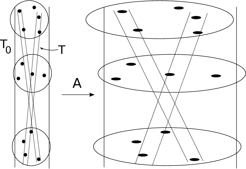
The proof has two phases: the first – and longer – reduces the proof to sets PP of a special form, which I call "quasi-product sets" in lack of a better term. This phase is elementary but tedious. One starts with a counter assumption: the union of the tubes in 𝒯\mathcal{T} can be covered by ≲δ−2​s\lesssim\delta^{-2s} and ≲δ−s\lesssim\delta^{-s} tubes at scales δ\delta and δ1/2\delta^{1/2}, respectively. Building on this information, one eventually finds a single δ1/2\delta^{1/2} tube T0T_{0} with the following properties. First, T0T_{0} contains a large number of points from PP. Second, each point in P∩T0P\cap T_{0} is incident to a large number of δ\delta-tubes TT, which are essentially contained in T0T_{0} (in particular, this can be used to find an upper bound on the total number of relevant tubes TT). After such a δ1/2\delta^{1/2}-tube T0T_{0} has been found, one applies an affine re-scaling AA, which essentially sends P∩T0P\cap T_{0} inside the unit square, and maps the δ\delta-tubes TT to δ1/2\delta^{1/2}-tubes, see Figure 1. Then, it turns out that A⁡(P∩T0)A(P\cap T_{0}) behaves like a quasi-product set, and has suspiciously many incidences with the δ1/2\delta^{1/2}-tubes A⁡(T)A(T).

Refer to caption
Figure 1. The tubes T0,TT_{0},T and the set P∩T0P\cap T_{0}, before and after the affine transformation AA. Explaining why A⁡(P∩T0)A(P\cap T_{0}) "behaves like a quasi-product set" would get too technical here, so I refer to Section 4.5 for more details.

At this point, it may seem like all the work has been fruitless: apart from changing scales from δ\delta to δ1/2\delta^{1/2}, the original incidence problem associated to PP and 𝒯\mathcal{T} has precisely the same numerology as the new incidence problem associated to A⁡(P∩T0)A(P\cap T_{0}) and the δ1/2\delta^{1/2}-tubes A⁡(T)A(T). However, it turns out that the problem is easier to solve (or at least make progress in) for quasi-product sets, because tools from additive combinatorics become available.

In the second phase, one proves an incidence theorem for quasi-product sets (see Proposition 4.36). This uses standard tools from additive combinatorics, such as the Plünnecke-Ruzsa inequalities and the Balog-Szemerédi-Gowers theorem. In the end, it turns out that the incidence problem for quasi-product sets is roughly equivalent to a discretised variant of Bourgain’s projection theorem, Theorem 1.12. Fortunately, Bourgain states and proves a suitable discretised variant of Theorem 1.12 in his paper [2], so the proof of Theorem 3.12 is completed by appealing to Theorem 5 in [2].

1.4. Some notation

An open ball in ℝd\mathbb{R}^{d} with centre xx and radius r>0r>0 will be denoted by B⁡(x,r)B(x,r). The Hausdorff measure and content of dimension tt will be denoted by ℋt\mathcal{H}^{t} and ℋ∞t\mathcal{H}^{t}_{\infty}, respectively. Given real numbers A,B>0A,B>0, the notation A≲BA\lesssim B means that A≤C​BA\leq CB for some constant C≥1C\geq 1. If the dependence of CC on a parameter pp needs to be emphasised, I will write A≲pBA\lesssim_{p}B. The notation A≳BA\gtrsim B means that B≲AB\lesssim A, and A∼BA\sim B stands for A≲B≲AA\lesssim B\lesssim A.

The notation A≲logBA\lesssim_{\log}B means that A≲logC⁡(1/δ)​BA\lesssim\log^{C}(1/\delta)B for some absolute constant C≥1C\geq 1, where δ>0\delta>0 is a "scale". The meaning of δ>0\delta>0 will be clear from the context, whenever the notation is used. The notations A≳logBA\gtrsim_{\log}B and A∼logBA\sim_{\log}B are then defined as above.

Given a bounded set F⊂ℝdF\subset\mathbb{R}^{d}, the notation N⁡(F,δ)N(F,\delta) stands for the least number of balls of radius δ\delta required to cover FF. The upper Minkowski dimension of FF is

dim¯​F:=lim supδ→0log⁡N⁡(F,δ)−log⁡δ.\overline{\dim}\,F:=\limsup_{\delta\to 0}\frac{\log N(F,\delta)}{-\log\delta}.

The packing dimension dimp\dim_{\mathrm{p}} is defined in (2.1) below.

1.5. Acknowledgements

I wish to thank the referees for reading the manuscript carefully and giving excellent comments; they helped me make the paper more readable.

2. Reductions to Minkowski dimension and compact sets

In this short section, I reduce the proofs of Theorems 1.7 and 1.13 to establishing analogous statements for Minkowski dimension (instead of packing dimension), and just for compact sets.

I start with reductions concerning Furstenberg sets. Let K⊂ℝ2K\subset\mathbb{R}^{2} be an arbitrary Furstenberg ss-set, and let SK⊂S1S_{K}\subset S^{1} be the associated set of unit vectors with ℋ1​(SK)>0\mathcal{H}^{1}(S_{K})>0. The definition of packing dimension is

(2.1) dimpK=inf{supidim¯​Fi:K⊂⋃iFi},\dim_{\mathrm{p}}K=\inf\left\{\sup_{i}\overline{\dim}\,F_{i}:K\subset\bigcup_{i}F_{i}\right\},

where the inf\inf is taken over all countable covers of KK with bounded sets FiF_{i}. Since taking closures does not affect the upper Minkowski dimension dim¯\overline{\dim}\,, one may restrict attention to covers by compact sets FiF_{i}. Now, given any ϵ>0\epsilon>0, I claim that one of the sets FiF_{i} is (essentially) a Furstenberg (s−ϵ)(s-\epsilon)-set. This is rather straightforward: since the sets FiF_{i} cover KK, one has

dimH[K∩Le]=supidimH[Fi∩Le],e∈SK,\dim_{\mathrm{H}}[K\cap L_{e}]=\sup_{i}\dim_{\mathrm{H}}[F_{i}\cap L_{e}],\qquad e\in S_{K},

so for any fixed e∈S1e\in S^{1}, it holds that ℋ∞s−ϵ​(Fi∩Le)>0\mathcal{H}^{s-\epsilon}_{\infty}(F_{i}\cap L_{e})>0 for some ii. Consequently, there exists ii such that ℋ∞s−ϵ​(Fi∩Le)≥c>0\mathcal{H}^{s-\epsilon}_{\infty}(F_{i}\cap L_{e})\geq c>0 for some c>0c>0 and for a positive set of vectors ee. Thus, FiF_{i} is a Furstenberg (s−ϵ)(s-\epsilon)-set. Since ϵ>0\epsilon>0 was arbitrary, it follows that it suffices to prove Theorem 1.7 for the Minkowski dimension dim¯\overline{\dim}\,, for compact sets KK, and under the extra assumption that

(2.2) ℋ∞s​(K∩Le)≥c>0,e∈SK.\mathcal{H}^{s}_{\infty}(K\cap L_{e})\geq c>0,\qquad e\in S_{K}.

As a slightly less obvious reduction, I claim that, without loss of generality, one may assume that the lines LeL_{e}, e∈SKe\in S_{K}, form a compact set. To formalise the statement, I recall the (standard) concept of point-line duality in the plane:

Definition 2.3 (Point-line duality).

The points in ℝ2\mathbb{R}^{2} are in one-to-one correspondence with non-vertical lines in ℝ2\mathbb{R}^{2} via the mapping

𝒟:(a,b)↦{y=a​x+b:x∈ℝ}.\mathcal{D}:(a,b)\mapsto\{y=ax+b:x\in\mathbb{R}\}.

For every set of points PP, define the set of lines ℒP:=𝒟⁡(P)={𝒟⁡(p):p∈P}\mathcal{L}_{P}:=\mathcal{D}(P)=\{\mathcal{D}(p):p\in P\}. Similarly, for a set ℒ\mathcal{L} of non-vertical lines ℒ\mathcal{L}, define the set of points Pℒ:=𝒟−1​(ℒ)P_{\mathcal{L}}:=\mathcal{D}^{-1}(\mathcal{L}). A family of lines will be called open/closed/compact etc. if the point set PℒP_{\mathcal{L}} has the same topological property. I will also write ℋt​(ℒ):=ℋt​(Pℒ)\mathcal{H}^{t}(\mathcal{L}):=\mathcal{H}^{t}(P_{\mathcal{L}}).

Remark 2.4.

Even though the family of lines 𝒟⁡(P)\mathcal{D}(P) and the planar set ∪{L:L∈𝒟⁡(P)}\cup\{L:L\in\mathcal{D}(P)\} are different objects, I will not differentiate between them in subsequent notation. In particular, if B⊂ℝ2B\subset\mathbb{R}^{2} is any set, the notation B∩𝒟⁡(P)B\cap\mathcal{D}(P) refers to ∪{B∩L:L∈𝒟⁡(P)}\cup\{B\cap L:L\in\mathcal{D}(P)\}.

Now, let ℒK:={Le:e∈SK}\mathcal{L}_{K}:=\{L_{e}:e\in S_{K}\}. Deleting a set of lines with sufficiently small measure, one may assume that every line in ℒK\mathcal{L}_{K} makes a positive (and uniformly bounded from below) angle with the yy-axis. Then PK:=PℒKP_{K}:=P_{\mathcal{L}_{K}} is a bounded graph, that is, a set of the form {(a,f⁡(a)):a∈A}\{(a,f(a)):a\in A\}, where A⊂ℝA\subset\mathbb{R} is a bounded set of positive length, and ff is a bounded function. Consider the compact line set

ℒ¯K:=ℒP¯K.\overline{\mathcal{L}}_{K}:=\mathcal{L}_{\overline{P}_{K}}.

Then every line L∈ℒ¯KL\in\overline{\mathcal{L}}_{K} has the property (2.2). This follows easily from the upper semi-continuity of Hausdorff content with respect to Hausdorff convergence and the compactness of KK. Namely, assume for a moment that L∈ℒ¯KL\in\overline{\mathcal{L}}_{K} is such that K∩LeK\cap L_{e} can be covered by finitely many open balls BiB_{i} with

∑id​(Bi)s<c.\sum_{i}d(B_{i})^{s}<c.

Choose a sequence of lines Lj∈ℒKL_{j}\in\mathcal{L}_{K} converging to LL locally in the Hausdorff metric. Then, using the compactness of KK, the sets K∩LjK\cap L_{j} can also be covered by the balls BiB_{i} for all jj large enough, contradicting (2.2).

The set P¯K\overline{P}_{K} may no longer be a graph, but it certainly satisfies ℋ1​(P¯K)>0\mathcal{H}^{1}(\overline{P}_{K})>0.

Definition 2.5 (Generalised Furstenberg ss-set).

Let 0<s<10<s<1. Assume that K⊂B⁡(0,1)⊂ℝ2K\subset B(0,1)\subset\mathbb{R}^{2} is a compact set, and ℒ\mathcal{L} is a compact set of lines with ℋ1​(ℒ)>0\mathcal{H}^{1}(\mathcal{L})>0 with the property that ℋ∞s​(K∩L)≥c>0\mathcal{H}^{s}_{\infty}(K\cap L)\geq c>0 for every L∈ℒL\in\mathcal{L}, and for some constant c>0c>0. Also, assume that every line L∈ℒL\in\mathcal{L} makes an angle ≥1/10\geq 1/10 with the yy-axis. Then KK is called a generalised Furstenberg ss-set.

By the previous discussion (and a simple coordinate-change, if necessary, to accommodate the angle requirement), the proof of Theorem 1.7 is now reduced to proving to following statement:

Theorem 2.6.

dim¯​K≥2​s+ϵ\overline{\dim}\,K\geq 2s+\epsilon for every generalised Furstenberg ss-set KK, where ϵ>0\epsilon>0 only depends on ss.

I now turn to the – much shorter – reduction related to the projection result, Theorem 1.13. The following observation is a special case Lemma 4.5 in [17]:

Lemma 2.7.

Assume that K⊂ℝ2K\subset\mathbb{R}^{2} is ℋ1\mathcal{H}^{1}-measurable with ℋ1​(K)>0\mathcal{H}^{1}(K)>0, and

dimH{e∈S1:dimpπe​(K)<σ}>β\dim_{\mathrm{H}}\{e\in S^{1}:\dim_{\mathrm{p}}\pi_{e}(K)<\sigma\}>\beta

for some σ,β>0\sigma,\beta>0. Then, there exists a compact set K′⊂KK^{\prime}\subset K with ℋ1​(K′)>0\mathcal{H}^{1}(K^{\prime})>0 such that ℋ1​(K′)>0\mathcal{H}^{1}(K^{\prime})>0 and

dimH{e∈S1:dim¯​πe​(K′)<σ}>β.\dim_{\mathrm{H}}\{e\in S^{1}:\overline{\dim}\,\pi_{e}(K^{\prime})<\sigma\}>\beta.

It follows immediately that it suffices to prove Theorem 1.13 for dim¯\overline{\dim}\, instead of dimp\dim_{\mathrm{p}}, and for compact sets KK with ℋ1​(K)>0\mathcal{H}^{1}(K)>0. Also, one may restrict attention to the case 0<ℋ1​(K)<∞0<\mathcal{H}^{1}(K)<\infty, since compact subsets with finite measure can always be found, and proving the theorem for any subset implies it for the whole set. For purposes of easy reference, I record the result explicitly:

Theorem 2.8.

Let 1/2<s<11/2<s<1. If K⊂ℝ2K\subset\mathbb{R}^{2} is a is compact with 0<ℋ1​(K)<∞0<\mathcal{H}^{1}(K)<\infty, then

dimH{e∈S1:dim¯​πe​(K)≤s}≤s−ϵ\dim_{\mathrm{H}}\{e\in S^{1}:\overline{\dim}\,\pi_{e}(K)\leq s\}\leq s-\epsilon

for some ϵ>0\epsilon>0 depending only on ss.

3. Proofs of Theorems 2.6 and 2.8

The proofs of both the main theorems are based on counter assumptions. If Theorem 2.6 fails, then for arbitrarily small ϵ>0\epsilon>0, there exists a generalised Furstenberg ss-set KF⊂ℝ2K_{F}\subset\mathbb{R}^{2} such that

(3.1) N⁡(KF,δ)≤δ−2​s−ϵN(K_{F},\delta)\leq\delta^{-2s-\epsilon}

for all small enough δ>0\delta>0, say 0<δ≤δ10<\delta\leq\delta_{1}. Recall that N⁡(K,δ)N(K,\delta) is the least number of balls of radius δ\delta required to cover KK. Similarly, if Theorem 2.8 fails, then for arbitrarily small ϵ>0\epsilon>0, there exists a number 1/2<s<11/2<s<1, a compact set Kπ⊂ℝ2K_{\pi}\subset\mathbb{R}^{2} with 0<ℋ1​(Kπ)<∞0<\mathcal{H}^{1}(K_{\pi})<\infty, and a set of vectors E⊂S1E\subset S^{1} with ℋs​(E)>0\mathcal{H}^{s}(E)>0 such that

(3.2) N⁡(πe​(Kπ),δ)≤δ−s−ϵ,e∈E,N(\pi_{e}(K_{\pi}),\delta)\leq\delta^{-s-\epsilon},\qquad e\in E,

for all 0<δ≤δ20<\delta\leq\delta_{2}.

The purpose of this section is to first pick the scale 0<δ≤δ0≤min⁡{δ1,δ2}0<\delta\leq\delta_{0}\leq\min\{\delta_{1},\delta_{2}\} so that the information from the counter assumptions (3.1) and (3.2) is as strong as possible. Then, at this scale δ>0\delta>0, the counter assumptions are employed to construct an "impossible" configuration of δ\delta-separated points and δ\delta-tubes. The "impossibility" of the configuration is finally deduced from an incidence result, Theorem 3.12. The proof of the incidence result is a separate story, which will occupy the remainder of the paper.

3.1. Finding the scale δ>0\delta>0

The scale δ\delta will only be chosen once, but it can be chosen arbitrarily small (by choosing δ0≤min⁡{δ1,δ2}\delta_{0}\leq\min\{\delta_{1},\delta_{2}\} very small). This will be useful – and implicitly assumed – countless times below. For example, I will always implicitly assume that δ−ϵ\delta^{-\epsilon} is far larger than various constants C≥1C\geq 1, which appear throughout the proof.

I start by recalling some basic facts about "discretising ss-dimensional sets". As far as I know, the following definition is due to Katz and Tao [9]:

Definition 3.3 ((δ,s,C)(\delta,s,C)-sets).

Fix δ,s>0\delta,s>0. A finite δ\delta-separated set P⊂ℝdP\subset\mathbb{R}^{d} is called a (δ,s,C)(\delta,s,C)-set, if

(3.4) |P∩B⁡(x,r)|≤C​(rδ)s|P\cap B(x,r)|\leq C\left(\frac{r}{\delta}\right)^{s}

for all x∈ℝdx\in\mathbb{R}^{d} and δ≤r≤1\delta\leq r\leq 1. Here and below, |⋅||\cdot| stands for cardinality.

An open ball of radius δ>0\delta>0 will be called a δ\delta-ball. A collection of δ\delta-balls will be called a (δ,s,C)(\delta,s,C)-set, if the centres of the balls form a (δ,s,C)(\delta,s,C)-set. The following proposition explains the rationale behind (δ,s,C)(\delta,s,C)-sets:

Proposition 3.5.

Let δ>0\delta>0, and let B⊂B⁡(0,1)⊂ℝ2B\subset B(0,1)\subset\mathbb{R}^{2} be a set with ℋ∞s​(B)=:κ>0\mathcal{H}^{s}_{\infty}(B)=:\kappa>0. Then, there exists a (δ,s,C)(\delta,s,C)-set P⊂BP\subset B with cardinality |P|≥(κ/C)⋅δ−s|P|\geq(\kappa/C)\cdot\delta^{-s}, where C≥1C\geq 1 is an absolute constant.

The proof is very close to that Frostman’s lemma; the details can be found in the appendix of [7]. Note that any (δ,s,C)(\delta,s,C)-set P⊂B⁡(0,1)P\subset B(0,1) satisfies |P|≤C​δ−s|P|\leq C\delta^{-s}. So, slightly informally, Proposition 3.3 says that sets B⊂B⁡(0,1)B\subset B(0,1) with ℋs​(B)>0\mathcal{H}^{s}(B)>0 contain (δ,s,C)(\delta,s,C)-sets with near-maximal cardinality.

Now, I will pick a suitable scale δ>0\delta>0. Recall the sets KFK_{F} and KπK_{\pi}. Since KFK_{F} is a generalised Furstenberg ss-set, it comes bundled with a compact set of lines ℒ\mathcal{L} with ℋ1​(ℒ)>0\mathcal{H}^{1}(\mathcal{L})>0. Clearly, one may also assume that ℋ1​(ℒ)<∞\mathcal{H}^{1}(\mathcal{L})<\infty, since a compact finite-measure subset ℒ′⊂ℒ\mathcal{L}^{\prime}\subset\mathcal{L} can be found, and then the pair KF,ℒ′K_{F},\mathcal{L}^{\prime} satisfies the same hypotheses as KF,ℒK_{F},\mathcal{L}.

Let KK be either one of the sets KπK_{\pi} or PℒP_{\mathcal{L}}, so that K⊂B⁡(0,1)K\subset B(0,1) and 0<ℋ1​(K)<∞0<\mathcal{H}^{1}(K)<\infty. I will treat ℋ1​(K)\mathcal{H}^{1}(K) as an absolute constant in the ≲\lesssim-notation below; in particular ℋ1​(K)∼1\mathcal{H}^{1}(K)\sim 1. Let μ\mu be a Frostman measure supported on KK, that is, μ⁡(K)=1\mu(K)=1 and μ⁡(B⁡(x,r))≲r\mu(B(x,r))\lesssim r for all balls B⁡(x,r)⊂ℝ2B(x,r)\subset\mathbb{R}^{2}. Next, let ℬ\mathcal{B} be an efficient δ0\delta_{0}-cover for KK, that is,

(3.6) sup{diam⁡B:B∈ℬ}≤δ0and∑B∈ℬdiam⁡(B)≲ℋ1​(K)∼1.\sup\{\operatorname{diam}B:B\in\mathcal{B}\}\leq\delta_{0}\quad\text{and}\quad\sum_{B\in\mathcal{B}}\operatorname{diam}(B)\lesssim\mathcal{H}^{1}(K)\sim 1.

One may assume that the diameters of the balls in ℬ\mathcal{B} are of the form 2−j2^{-j}, j∈ℕj\in\mathbb{N}. For 2−j≤δ02^{-j}\leq\delta_{0}, set ℬj:={B∈ℬ:diam⁡(B)=2−j}\mathcal{B}_{j}:=\{B\in\mathcal{B}:\operatorname{diam}(B)=2^{-j}\}, and observe that

∑2−j≤δ0∑B∈ℬjμ⁡(B)≥μ⁡(K)=1.\sum_{2^{-j}\leq\delta_{0}}\sum_{B\in\mathcal{B}_{j}}\mu(B)\geq\mu(K)=1.

In particular, there exists an index j∈ℕj\in\mathbb{N} with 2−j≤δ02^{-j}\leq\delta_{0} and

(3.7) ∑B∈ℬjμ⁡(B)≳1(j−j0+1)2.\sum_{B\in\mathcal{B}_{j}}\mu(B)\gtrsim\frac{1}{(j-j_{0}+1)^{2}}.

Here j0∈ℕj_{0}\in\mathbb{N} is the smallest number with 2−j0≤δ02^{-j_{0}}\leq\delta_{0}. Now, I set

δ:=2−2​j,\delta:=2^{-2j},

so that δ1/2=2−j\delta^{1/2}=2^{-j}. Note that δ1/2≤δ0\delta^{1/2}\leq\delta_{0}. In particular, (3.7) implies that

(3.8) ∑B∈ℬjμ(B)≳log1.\sum_{B\in\mathcal{B}_{j}}\mu(B)\gtrsim_{\log}1.

Observe that |ℬj|≲δ−1/2|\mathcal{B}_{j}|\lesssim\delta^{-1/2} by (3.6), and on the other hand every ball B∈ℬjB\in\mathcal{B}_{j} satisfies μ⁡(B)≲δ1/2\mu(B)\lesssim\delta^{1/2}. Thus, (3.8) implies that there are ∼logδ−1/2\sim_{\log}\delta^{-1/2} balls in ℬj\mathcal{B}_{j}, denoted by ℬjG\mathcal{B}_{j}^{G}, such that

(3.9) μ(B)≳logδ1/2,B∈ℬjG.\mu(B)\gtrsim_{\log}\delta^{1/2},\qquad B\in\mathcal{B}_{j}^{G}.

Discarding a few balls if necessary, one may assume that

(3.10) dist(B,B′)≥δ−1/2,B,B′∈ℬjG.\operatorname{dist}(B,B^{\prime})\geq\delta^{-1/2},\qquad B,B^{\prime}\in\mathcal{B}_{j}^{G}.

For each ball B∈BjGB\in B_{j}^{G}, choose a (δ,1,C)(\delta,1,C)-set PB⊂BP_{B}\subset B with C∼1C\sim 1 and |PB|≳logδ−1/2|P_{B}|\gtrsim_{\log}\delta^{-1/2}. This is possible by Proposition 3.5, since (3.9) and the linear growth of μ\mu imply that ℋ∞1(B∩K)≳logδ1/2\mathcal{H}_{\infty}^{1}(B\cap K)\gtrsim_{\log}\delta^{1/2}. Write

P:=⋃B∈ℬjGPB.P:=\bigcup_{B\in\mathcal{B}_{j}^{G}}P_{B}.

Then |P|∼logδ−1|P|\sim_{\log}\delta^{-1}, and PB=B∩PP_{B}=B\cap P for B∈ℬjGB\in\mathcal{B}_{j}^{G}. I will now verify that PP is a (δ,1,C)(\delta,1,C)-set for some C∼log1C\sim_{\log}1. Fix x∈Px\in P and r≥δr\geq\delta, let B∈ℬjGB\in\mathcal{B}_{j}^{G} be the unique ball with x∈PBx\in P_{B}. There are two cases to consider: if δ≤r≤δ1/2\delta\leq r\leq\delta^{1/2}, one needs only note that |P∩B⁡(x,r)|=|PB∩B⁡(x,r)||P\cap B(x,r)|=|P_{B}\cap B(x,r)| by (3.10), and recall that PBP_{B} is a (δ,1,C)(\delta,1,C)-set with C∼1C\sim 1. So, let r≥δ1/2r\geq\delta^{1/2}. This time, if B⁡(x,r)∩B′≠∅B(x,r)\cap B^{\prime}\neq\emptyset for some ball B′∈ℬjGB^{\prime}\in\mathcal{B}_{j}^{G}, then rr is large enough to ensure that B′⊂B⁡(x,2​r)B^{\prime}\subset B(x,2r). Hence, by |P∩B′|≲δ−1/2|P\cap B^{\prime}|\lesssim\delta^{-1/2} for B′∈ℬjGB^{\prime}\in\mathcal{B}_{j}^{G}, and (3.9), and the disjointness of the balls in ℬjG\mathcal{B}_{j}^{G}, one obtains

|P∩B(x,r)|≲δ−1/2∑B′∈ℬjGB′∩B⁡(x,r)≠∅μ⁡(B′)μ⁡(B′)≲logδ−1∑B′∈ℬjGB′⊂B⁡(x,2​r)μ(B′)≤μ⁡(B⁡(x,2​r))δ≲rδ.|P\cap B(x,r)|\lesssim\delta^{-1/2}\mathop{\sum_{B^{\prime}\in\mathcal{B}_{j}^{G}}}_{B^{\prime}\cap B(x,r)\neq\emptyset}\frac{\mu(B^{\prime})}{\mu(B^{\prime})}\lesssim_{\log}\delta^{-1}\mathop{\sum_{B^{\prime}\in\mathcal{B}_{j}^{G}}}_{B^{\prime}\subset B(x,2r)}\mu(B^{\prime})\leq\frac{\mu(B(x,2r))}{\delta}\lesssim\frac{r}{\delta}.

I recap the main achievements so far. For a suitable scale δ≤δ02\delta\leq\delta_{0}^{2}, a (δ,1,C)(\delta,1,C)-set P⊂K∈{Kπ,Pℒ}P\subset K\in\{K_{\pi},P_{\mathcal{L}}\} has now been constructed with C∼log1C\sim_{\log}1, along with a family of δ1/2\delta^{1/2}-balls ℬ\mathcal{B} such that

  • (P1)

    |P|∼logδ−1|P|\sim_{\log}\delta^{-1}, and |ℬ|≲δ−1/2|\mathcal{B}|\lesssim\delta^{-1/2},

  • (P2)

    P⊂⋃B∈ℬBP\subset\bigcup_{B\in\mathcal{B}}B.

3.2. Finding δ\delta-tubes

Next, relying on the counter assumptions (3.1) and (3.2), I will accompany PP with a finite family of δ\delta-tubes. For technical reasons, I will consider two types of δ\delta-tubes in this paper: the ordinary ones, which are (δ/2)(\delta/2)-neighbourhoods of lines in ℝ2\mathbb{R}^{2}, and then the dyadic ones, which I now proceed to define:

Definition 3.11 (Dyadic tubes).

For δ=2−k\delta=2^{-k}, k≥0k\geq 0, a dyadic δ\delta-tube is a set of the form 𝒟⁡(Q)\mathcal{D}(Q), where Q⊂[0,1)2Q\subset[0,1)^{2} is a dyadic square of side-length δ\delta, and 𝒟\mathcal{D} is the point-line duality mapping from Definition 2.3. One should view 𝒟⁡(Q)\mathcal{D}(Q) here as a set of points in ℝ2\mathbb{R}^{2}, not as a family of lines, see Remark 2.4. The slope of a dyadic δ\delta-tube T=𝒟([a+δ)×[b+δ))T=\mathcal{D}([a+\delta)\times[b+\delta)) is defined fo be s⁡(T):=as(T):=a (which is the actual slope of the line 𝒟⁡(a,b)⊂T\mathcal{D}(a,b)\subset T).

The definition above is convenient for the reason that dyadic tubes have a dyadic structure (unlike ordinary tubes). For dyadic numbers 0<δ1<δ2<10<\delta_{1}<\delta_{2}<1, the δ2\delta_{2}-parent of a δ1\delta_{1}-tube T1=𝒟⁡(Q1)T_{1}=\mathcal{D}(Q_{1}) is the unique tube T2=𝒟⁡(Q2)T_{2}=\mathcal{D}(Q_{2}) such that Q2Q_{2} is a dyadic square of side-length δ2\delta_{2} containing Q1Q_{1}. The δ1\delta_{1}-children of a δ2\delta_{2}-tube are defined in the obvious way: note that a δ1\delta_{1}-tube T1T_{1} is the child of a δ2\delta_{2}-tube T2T_{2}, if and only if T1⊂T2T_{1}\subset T_{2}. Given a collection of δ1\delta_{1}-tubes 𝒯\mathcal{T}, I write N⁡(𝒯,δ2)N(\mathcal{T},\delta_{2}) for the cardinality of the family of δ2\delta_{2}-parents of the tubes in 𝒯\mathcal{T} (that is, minimal family of δ2\delta_{2}-tubes containing all the tubes in 𝒯\mathcal{T}).

From geometric intents and purposes, dyadic tubes are locally very similar to ordinary tubes: if TT is a dyadic δ\delta-tube, then the intersection T∩B⁡(0,R)T\cap B(0,R) is contained in an ordinary CR​δC_{R}\delta-tube with the same slope, for some constant CR≥1C_{R}\geq 1 depending only on RR. Conversely, an ordinary δ\delta-tube can be covered by a bounded number of dyadic δ\delta-tubes with nearly the same slope (with an error of ≲δ\lesssim\delta).

Assume that 𝒯p\mathcal{T}_{p} is a collection of dyadic δ\delta-tubes, each containing a point p∈ℝ2p\in\mathbb{R}^{2}, and let 0<s<10<s<1. Then 𝒯p\mathcal{T}_{p} is called a (δ,s,C)(\delta,s,C)-set, if the set of slopes s⁡(𝒯p):={s⁡(T):T∈𝒯p}s(\mathcal{T}_{p}):=\{s(T):T\in\mathcal{T}_{p}\} is a (δ,s,C)(\delta,s,C)-subset of ℝ\mathbb{R}. The same definition is used, if pp is a δ\delta-ball instead of a point, and "containing pp" is replaced by "intersecting pp".

Similarly, a family of ordinary δ\delta-tubes, all containing a common point, is called a (δ,s,C)(\delta,s,C)-set, if the directions of the tubes (on S1S^{1}) form a (δ,s,C)(\delta,s,C)-set.

As stated above Definition 3.11, the plan is to use the counter assumptions (3.1) and (3.2) to accompany PP with a finite family of dyadic δ\delta-tubes 𝒯\mathcal{T}. Finding 𝒯\mathcal{T} is a somewhat lengthy task, so I start by clarifying: what exactly is required of these tubes to end up with a contradiction? In brief, the tubes need violate the next theorem:

Theorem 3.12.

Given 0<s<10<s<1, there exists an ϵ=ϵ⁡(s)>0\epsilon=\epsilon(s)>0 such that the following holds for small enough dyadic numbers δ>0\delta>0 (depending only on ss). Assume that P⊂B⁡(0,1)⊂ℝ2P\subset B(0,1)\subset\mathbb{R}^{2} is a (δ,1,δ−ϵ)(\delta,1,\delta^{-\epsilon})-set with cardinality |P|≥δ−1+ϵ|P|\geq\delta^{-1+\epsilon} and assume that

(3.13) N(P,δ1/2)≤δ−1/2−ϵ.N(P,\delta^{1/2})\leq\delta^{-1/2-\epsilon}.

Assume that 𝒯\mathcal{T} is a collection of dyadic δ\delta-tubes such that for every p∈Pp\in P, there exists a sub-family 𝒯p⊂{T∈𝒯:p∈T}\mathcal{T}_{p}\subset\{T\in\mathcal{T}:p\in T\}, which is a (δ,s,δ−ϵ)(\delta,s,\delta^{-\epsilon})-set of cardinality |𝒯p|≥δ−s+ϵ|\mathcal{T}_{p}|\geq\delta^{-s+\epsilon}. Then either

(3.14) |𝒯|≥δ−2​s−ϵorN⁡(𝒯,δ1/2)≥δ−s−ϵ.|\mathcal{T}|\geq\delta^{-2s-\epsilon}\quad\text{or}\quad N(\mathcal{T},\delta^{1/2})\geq\delta^{-s-\epsilon}.

Note that the assumptions of Theorem 3.12, in particular (3.13), are valid for the set PP constructed earlier, by properties (P1)–(P2). So, to prove Theorems 2.6 and 2.8, it remains to use (3.1) and (3.2) to find a family of dyadic δ\delta-tubes 𝒯\mathcal{T} which violates Theorem 3.12. I first need to record a few easy geometric lemmas about points and dyadic δ\delta-tubes:

Lemma 3.15.

Assume that 𝒯p\mathcal{T}_{p} is a collection of dyadic δ\delta-tubes, each containing a point p∈B⁡(0,1)p\in B(0,1). Then |s⁡(𝒯p)|∼|𝒯p||s(\mathcal{T}_{p})|\sim|\mathcal{T}_{p}|.

Proof.

Write S:=s⁡(𝒯p)S:=s(\mathcal{T}_{p}). Clearly |S|≤|𝒯p||S|\leq|\mathcal{T}_{p}|, so it suffices to prove that |𝒯p|≲|S||\mathcal{T}_{p}|\lesssim|S|. To this end, I will show that only four tubes in 𝒯p\mathcal{T}_{p} can share a common slope. Assume that a∈Sa\in S, and T1=𝒟([a,a+δ)×[b1,b1+δ))T_{1}=\mathcal{D}([a,a+\delta)\times[b_{1},b_{1}+\delta)) and T2=𝒟([a,a+δ)×[b2,b2+δ))T_{2}=\mathcal{D}([a,a+\delta)\times[b_{2},b_{2}+\delta)) both belong to 𝒯p\mathcal{T}_{p}, so that p=(px,py)∈T1∩T2p=(p_{x},p_{y})\in T_{1}\cap T_{2}. By definition of T1,T2T_{1},T_{2}, this means that there exist numbers a′,b1′,a′′,b2′′a^{\prime},b_{1}^{\prime},a^{\prime\prime},b_{2}^{\prime\prime} with max⁡{|a′−a|,|a′′−a|,|b1′−b1|,|b2′′−b2|}<δ\max\{|a^{\prime}-a|,|a^{\prime\prime}-a|,|b_{1}^{\prime}-b_{1}|,|b_{2}^{\prime\prime}-b_{2}|\}<\delta such that

py=a′​px+b1′andpy=a′′​px=b2′′.p_{y}=a^{\prime}p_{x}+b_{1}^{\prime}\quad\text{and}\quad p_{y}=a^{\prime\prime}p_{x}=b_{2}^{\prime\prime}.

It follows that |b1−b2|≤|px|​|a′−a′′|+2​δ<4​δ|b_{1}-b_{2}|\leq|p_{x}||a^{\prime}-a^{\prime\prime}|+2\delta<4\delta. This completes the proof. ∎

Lemma 3.16.

Assume that 0<δ1<δ20<\delta_{1}<\delta_{2} are dyadic numbers, p∈B⁡(0,1)p\in B(0,1), and T0=𝒟(Q0)=𝒟([a,a+δ2)×[b,b+δ2))T_{0}=\mathcal{D}(Q_{0})=\mathcal{D}([a,a+\delta_{2})\times[b,b+\delta_{2})) is a dyadic δ2\delta_{2}-tube. Further, assume that 𝒯p\mathcal{T}_{p} is a (δ1,s,C)(\delta_{1},s,C)-set of dyadic δ1\delta_{1}-tubes TT with p∈T⊂T0p\in T\subset T_{0}. Then |𝒯p|≲C​(δ2/δ1)s|\mathcal{T}_{p}|\lesssim C(\delta_{2}/\delta_{1})^{s}.

Proof.

Let 𝒬p\mathcal{Q}_{p} be the collection of dyadic δ1\delta_{1}-squares such that 𝒯p={𝒟⁡(Q):Q∈𝒬p}\mathcal{T}_{p}=\{\mathcal{D}(Q):Q\in\mathcal{Q}_{p}\}. Then Q⊂Q0Q\subset Q_{0}, Q∈𝒬pQ\in\mathcal{Q}_{p}, by the assumption T⊂T0T\subset T_{0}, T∈𝒯pT\in\mathcal{T}_{p}. Hence s⁡(𝒯p)s(\mathcal{T}_{p}) is a (δ1,s,C)(\delta_{1},s,C)-subset of [a,a+δ2)[a,a+\delta_{2}), and consequently |s⁡(𝒯p)|≤C​(δ2/δ1)s|s(\mathcal{T}_{p})|\leq C(\delta_{2}/\delta_{1})^{s}. The previous lemma completes the proof.∎

Lemma 3.17.

Assume that P⊂B⁡(0,1)P\subset B(0,1) is a set and 0<δ1≤δ20<\delta_{1}\leq\delta_{2} are dyadic numbers. Assume that a2∈δ2​ℤa_{2}\in\delta_{2}\mathbb{Z}, and PP can be covered by M∈ℕM\in\mathbb{N} dyadic δ2\delta_{2}-tubes 𝒟([a2,a2+δ2)×[bj,bj+δ2))\mathcal{D}([a_{2},a_{2}+\delta_{2})\times[b_{j},b_{j}+\delta_{2})) with fixed slope a2a_{2}. Then the collection of all dyadic δ1\delta_{1}-tubes, which intersect PP and have slope in [a2,a2+δ2)[a_{2},a_{2}+\delta_{2}), can be covered by ≲M\lesssim M dyadic δ2\delta_{2}-tubes with slope a2a_{2}.

Proof.

Assume that 𝒟([a1,a1+δ1)×[b1,b1+δ1))\mathcal{D}([a_{1},a_{1}+\delta_{1})\times[b_{1},b_{1}+\delta_{1})) is a δ1\delta_{1}-tube with slope a1∈[a2,a2+δ2)a_{1}\in[a_{2},a_{2}+\delta_{2}), which intersects PP at a point p=(px,py)p=(p_{x},p_{y}). This means that py=a1′​px+b1′p_{y}=a_{1}^{\prime}p_{x}+b_{1}^{\prime} for some |a1′−a1|<δ1|a_{1}^{\prime}-a_{1}|<\delta_{1}, and consequently |a1′−a2|≤2​δ2|a_{1}^{\prime}-a_{2}|\leq 2\delta_{2}. By assumption, pp is also covered by one of the dyadic δ2\delta_{2}-tubes 𝒟([a2,a2+δ2)×[bj,bj+δ2))\mathcal{D}([a_{2},a_{2}+\delta_{2})\times[b_{j},b_{j}+\delta_{2})), 1≤j≤M1\leq j\leq M, which implies that py=a2′​px+bj′p_{y}=a_{2}^{\prime}p_{x}+b_{j}^{\prime} for some |a2′−a2|<δ2|a_{2}^{\prime}-a_{2}|<\delta_{2} and |bj′−bj|<δ2|b_{j}^{\prime}-b_{j}|<\delta_{2}. It follows that

|b1′−bj′|=|px|​|a1′−a2′|≤3​δ2,|b_{1}^{\prime}-b_{j}^{\prime}|=|p_{x}||a_{1}^{\prime}-a_{2}^{\prime}|\leq 3\delta_{2},

and consequently |b1−bj|≤5​δ2|b_{1}-b_{j}|\leq 5\delta_{2}. Now, the δ2\delta_{2}-tubes of the form 𝒟([a2,a2+δ)×[b,b+δ2))\mathcal{D}([a_{2},a_{2}+\delta)\times[b,b+\delta_{2})) with |b−bj|≤5​δ|b-b_{j}|\leq 5\delta for some 1≤j≤M1\leq j\leq M, form the desired cover. ∎

Now, finally, everything is set up to accompany PP with a family of dyadic δ\delta-tubes 𝒯\mathcal{T}. The process is slightly different in the cases K=KπK=K_{\pi} and K=PℒK=P_{\mathcal{L}}.

3.2.1. The case P⊂K=KπP\subset K=K_{\pi}

Here we use the counter assumption (3.2), restated below:

(3.18) N⁡(πe​(Kπ),δ)≤δ−s−ϵ,e∈E, 0<δ≤δ0,N(\pi_{e}(K_{\pi}),\delta)\leq\delta^{-s-\epsilon},\quad e\in E,\>0<\delta\leq\delta_{0},

where ℋs​(E)>0\mathcal{H}^{s}(E)>0. The plan is to find a (δ,s)(\delta,s)-subset E′⊂EE^{\prime}\subset E of near-maximal cardinality and use (3.18) to cover P⊂KπP\subset K_{\pi} by a small family of dyadic δ\delta-tubes 𝒯e\mathcal{T}_{e} (nearly) perpendicular to ee for every e∈E′e\in E^{\prime}.

Recall that both δ\delta and δ1/2\delta^{1/2} are dyadic numbers. Let Eδ⊂δ​ℤE_{\delta}\subset\delta\mathbb{Z} be a (δ,s,C)(\delta,s,C)-set of slopes almost perpendicular to the vectors in EE: more precisely, if θ∈Eδ\theta\in E_{\delta}, the requirement is that any line with slope θ\theta is perpendicular to some vector in E⁡(10​δ)E(10\delta) (the 10​δ10\delta-neighbourhood is only needed to facilitate Eδ⊂δ​ℤE_{\delta}\subset\delta\mathbb{Z}). By Proposition 3.3 applied to EE and some easy tinkering, one can choose EδE_{\delta} with |Eδ|∼δ−s|E_{\delta}|\sim\delta^{-s} (the implicit constants naturally depend on ℋ∞s​(E)>0\mathcal{H}^{s}_{\infty}(E)>0, which will be treated as an absolute constant). Inequality (3.18) then implies that for every θ∈Eδ\theta\in E_{\delta}, the set KπK_{\pi} can be covered by ≲δ−s−ϵ\lesssim\delta^{-s-\epsilon} dyadic δ\delta-tubes 𝒯θ\mathcal{T}_{\theta} with slope θ\theta. Without loss of generality, all tubes will be assumed to intersect KπK_{\pi}. Let

𝒯:=⋃θ∈Eδ𝒯θ.\mathcal{T}:=\bigcup_{\theta\in E_{\delta}}\mathcal{T}_{\theta}.

Then 𝒯\mathcal{T} is a collection of dyadic δ\delta-tubes such that

  • (T1)

    |𝒯|≲δ−2​s−ϵ|\mathcal{T}|\lesssim\delta^{-2s-\epsilon},

  • (T2)

    for every point p∈P⊂Kp\in P\subset K, there is a (δ,s,C)(\delta,s,C)-subset 𝒯p⊂{T∈𝒯:p∈T}\mathcal{T}_{p}\subset\{T\in\mathcal{T}:p\in T\} of cardinality |𝒯p|∼δ−s|\mathcal{T}_{p}|\sim\delta^{-s}.

  • (T3)

    N⁡(𝒯,δ1/2)≲δ−s−ϵN(\mathcal{T},\delta^{1/2})\lesssim\delta^{-s-\epsilon}.

Here (T1) follows from |Eδ|∼δ−s|E_{\delta}|\sim\delta^{-s} and |𝒯θ|≲δ−s−ϵ|\mathcal{T}_{\theta}|\lesssim\delta^{-s-\epsilon}. To see the (T2), fix p∈P⊂K=Kπp\in P\subset K=K_{\pi} and observe that p∈Tp\in T for some tube T∈𝒯θT\in\mathcal{T}_{\theta}, for every θ∈Eδ\theta\in E_{\delta}. The family 𝒯p\mathcal{T}_{p} can be picked among those tubes TT. The the claim (T3) requires a bit of extra work. I first recall the following basic estimate:

Proposition 3.19.

Assume that K⊂B⁡(0,1)K\subset B(0,1) with ℋ1​(K)>0\mathcal{H}^{1}(K)>0 and 0<t<10<t<1. Then

N({e∈S1:N(πe(K),δ)≤δ−t},δ)≲logδ−t,N(\{e\in S^{1}:N(\pi_{e}(K),\delta)\leq\delta^{-t}\},\delta)\lesssim_{\log}\delta^{-t},

where the implicit constants depend on ℋ1​(K)\mathcal{H}^{1}(K).

This is, for instance, inequality (1.2) in [18], and the proof can be found on p. 9 of the same paper. The proposition also easily follows from Lemma 4.1 below. Now, apply Proposition 3.19 with t=s+ϵt=s+\epsilon, at scale δ1/2\delta^{1/2}, and the set KπK_{\pi}. The conclusion is that

(3.20) N(Eδ,δ1/2)≲N({e∈S1:N(πe(Kπ),δ1/2)≤Cδ−(s+ϵ)/2},δ1/2)≲logδ−(s+ϵ)/2.N(E_{\delta},\delta^{1/2})\lesssim N(\{e\in S^{1}:N(\pi_{e}(K_{\pi}),\delta^{1/2})\leq C\delta^{-(s+\epsilon)/2}\},\delta^{1/2})\lesssim_{\log}\delta^{-(s+\epsilon)/2}.

The first inequality follows from the fact that if θ∈Eδ​(δ1/2)\theta\in E_{\delta}(\delta^{1/2}), then a unit vector eθe_{\theta} parallel to a line with slope θ\theta lies at distance ≲δ1/2\lesssim\delta^{1/2} from some vector e∈E⟂e\in E^{\perp}. Then, if eθ⟂,e⟂e_{\theta}^{\perp},e^{\perp} are perpendicular to eθ,ee_{\theta},e, one has |eθ⟂−e⟂|≲δ1/2|e_{\theta}^{\perp}-e^{\perp}|\lesssim\delta^{1/2}, and

(3.21) N(πeθ⟂(Kπ),δ1/2)≲N(πe⟂(Kπ),δ1/2)≤δ−(s+ϵ)/2N(\pi_{e_{\theta}^{\perp}}(K_{\pi}),\delta^{1/2})\lesssim N(\pi_{e^{\perp}}(K_{\pi}),\delta^{1/2})\leq\delta^{-(s+\epsilon)/2}

by the definition of EE (and δ1/2≤δ0\delta^{1/2}\leq\delta_{0}). This means that eθ⟂e_{\theta}^{\perp} belongs to the set in the middle of (3.20) for large enough C≥1C\geq 1, which implies the first inequality of (3.20) for the vectors eθe_{\theta}, θ∈Eδ\theta\in E_{\delta} – and then for the points θ∈Eδ\theta\in E_{\delta}.

With (3.20) in hand, pick a collection {θj}j∈𝒥⊂δ1/2​ℤ\{\theta_{j}\}_{j\in\mathcal{J}}\subset\delta^{1/2}\mathbb{Z} such that |𝒥|≲δ−(s+ϵ)/2|\mathcal{J}|\lesssim\delta^{-(s+\epsilon)/2} and EδE_{\delta} is contained in the union of the dyadic intervals [θj,θj+δ1/2)[\theta_{j},\theta_{j}+\delta^{1/2}). The numbers θj\theta_{j} can be picked at distance ≤δ1/2\leq\delta^{1/2} from some point in EδE_{\delta}, so (3.21) applies with θ=θj\theta=\theta_{j}: the conclusion is that KπK_{\pi} can be covered by ≲δ−(s+ϵ)/2\lesssim\delta^{-(s+\epsilon)/2} dyadic δ1/2\delta^{1/2}-tubes with slope θj\theta_{j}. Consequently, by Lemma 3.17, all the tubes in the families 𝒯θ\mathcal{T}_{\theta}, with θ∈Eδ∩[θj,θj+δ1/2)\theta\in E_{\delta}\cap[\theta_{j},\theta_{j}+\delta^{1/2}), can be covered by ≲δ−(s+ϵ)/2\lesssim\delta^{-(s+\epsilon)/2} dyadic δ1/2\delta^{1/2}-tubes of slope θj\theta_{j}. It follows that all the tubes in 𝒯\mathcal{T} can be covered by ≲δ−(s+ϵ)/2⋅δ−(s+ϵ)/2=δ−s−ϵ\lesssim\delta^{-(s+\epsilon)/2}\cdot\delta^{-(s+\epsilon)/2}=\delta^{-s-\epsilon} dyadic δ1/2\delta^{1/2}-tubes, as claimed in (T3).

3.2.2. The case P⊂K=PℒP\subset K=P_{\mathcal{L}}

This case is simpler: again, the aim is to find a family of dyadic δ\delta-tubes 𝒯\mathcal{T} satisfying the conditions (T1)–(T3). Recall the main counter assumption (3.1):

(3.22) N⁡(KF,δ)≤δ−2​s−ϵ,0<δ≤δ0.N(K_{F},\delta)\leq\delta^{-2s-\epsilon},\qquad 0<\delta\leq\delta_{0}.

Also, recall that ℒ\mathcal{L} is a compact set of lines LL, which form a large angle with the yy-axis, and with the property that ℋ∞s​(KF∩L)≥c>0\mathcal{H}^{s}_{\infty}(K_{F}\cap L)\geq c>0. By (P1), P⊂PℒP\subset P_{\mathcal{L}} is a (δ,1,C)(\delta,1,C)-set with C∼log1C\sim_{\log}1 of cardinality |P|∼logδ−1|P|\sim_{\log}\delta^{-1}.

I record a small observation about the point-line duality:

Lemma 3.23.

Assume that (c,d)∈𝒟⁡(a,b)(c,d)\in\mathcal{D}(a,b). Then (a,b)∈𝒟⁡(−c,d)(a,b)\in\mathcal{D}(-c,d).

Proof.

By assumption d=a​c+bd=ac+b, or b=(−c)​a+db=(-c)a+d. Hence (a,b)∈𝒟⁡(−c,d)(a,b)\in\mathcal{D}(-c,d). ∎

Note that Lp:=𝒟⁡(p)∈ℒL_{p}:=\mathcal{D}(p)\in\mathcal{L} for all p∈P⊂Pℒp\in P\subset P_{\mathcal{L}}. It follows from ℋ∞s​(KF∩Lp)≥c\mathcal{H}^{s}_{\infty}(K_{F}\cap L_{p})\geq c and Proposition 3.3 that KF∩LpK_{F}\cap L_{p} contains a (δ,s,C)(\delta,s,C)-set with C∼1C\sim 1 and cardinality ∼δ−s\sim\delta^{-s} (I treat cc as an absolute constant). Let 𝒬p′={(ai,ai+δ]×[bi,bi+δ)}i∈ℐ\mathcal{Q}_{p}^{\prime}=\{(a_{i},a_{i}+\delta]\times[b_{i},b_{i}+\delta)\}_{i\in\mathcal{I}} be the collection of (not quite dyadic) δ\delta-squares of the form (a,a+δ]×[b,b+δ)(a,a+\delta]\times[b,b+\delta) with a,b∈δ​ℤa,b\in\delta\mathbb{Z}, which contain a point in the said (δ,s,C)(\delta,s,C)-set on KF∩LpK_{F}\cap L_{p}. Then 𝒬p:={[−ai−δ,ai)×[bi,bi+δ)}i∈ℐ\mathcal{Q}_{p}:=\{[-a_{i}-\delta,a_{i})\times[b_{i},b_{i}+\delta)\}_{i\in\mathcal{I}} is a collection of dyadic squares. Since LpL_{p} is quantitatively non-vertical, the numbers aia_{i} form a (δ,s,C)(\delta,s,C)-set, and hence 𝒯p:={𝒟⁡(Q):Q∈𝒬p}\mathcal{T}_{p}:=\{\mathcal{D}(Q):Q\in\mathcal{Q}_{p}\} is a (δ,s,C)(\delta,s,C)-set of dyadic δ\delta-tubes by definition. Each tube 𝒟([−ai−δ,ai)×[bi,bi+δ))∈𝒯p\mathcal{D}([-a_{i}-\delta,a_{i})\times[b_{i},b_{i}+\delta))\in\mathcal{T}_{p} moreover contains pp, since (ai,ai+δ]×[bi,bi+δ)(a_{i},a_{i}+\delta]\times[b_{i},b_{i}+\delta) contains a point (x1,x2)∈Lp=𝒟⁡(p)(x_{1},x_{2})\in L_{p}=\mathcal{D}(p) by definition, and then

p∈𝒟(−x1,x2)∈𝒟([−ai−δ,ai)×[bi,bi+δ))p\in\mathcal{D}(-x_{1},x_{2})\in\mathcal{D}([-a_{i}-\delta,a_{i})\times[b_{i},b_{i}+\delta))

by Lemma 3.23. Writing

𝒯:=⋃p∈P𝒯p,\mathcal{T}:=\bigcup_{p\in P}\mathcal{T}_{p},

the condition (T2) is automatically valid. Note that 𝒯\mathcal{T} consists of 𝒟\mathcal{D}-images of δ\delta-squares QQ meeting {(−x,y):(x,y)∈KF}\{(-x,y):(x,y)\in K_{F}\}. Hence |𝒯|≲δ−2​s−ϵ|\mathcal{T}|\lesssim\delta^{-2s-\epsilon} by (3.22), which gives (T1). Finally, all these δ\delta-squares can be covered by ≲δ−s−ϵ/2\lesssim\delta^{-s-\epsilon/2} dyadic squares of side-length δ1/2\delta^{1/2}, by (3.22) at scale δ1/2\delta^{1/2}. This gives N⁡(𝒯,δ1/2)≲δ−s−ϵ/2N(\mathcal{T},\delta^{1/2})\lesssim\delta^{-s-\epsilon/2}, which is a little bit better than (T3).

3.3. Concluding the proofs of Theorems 2.6 and 2.8

In both cases K=KπK=K_{\pi} and K=𝒫ℒK=\mathcal{P}_{\mathcal{L}}, a finite set PP and a collection of tubes 𝒯\mathcal{T} have now been found, satisfying (P1)–(P2) and (T1)–(T3), respectively. The counter assumptions (3.1) and (3.2) were heavily used. Now, to conclude the proofs of both Theorems 2.6 and 2.8, it suffices to show that PP can 𝒯\mathcal{T} cannot exist, for sufficiently small ϵ>0\epsilon>0. This follows from Theorem 3.12. Indeed, we already observed earlier that PP satisfies the hypotheses of Theorem 3.12, by (P1)–(P2). Moreover, the condition (T2) is even slightly better than what Theorem 3.12 requires from 𝒯\mathcal{T}, and conditions (T1) and (T3) literally state that the main conclusion (3.14) of Theorem 3.12 fails (assuming that ϵ>0\epsilon>0 is sufficiently small). So, a contradiction has been reached, and the proofs of Theorems 2.6 and 2.8 are complete.

4. An incidence bound for points and tubes

The purpose of this section is to prove Theorem 3.12, stated below as Theorem 4.3 for convenience. I start with a simple – and well-known – incidence bound: heuristically, Theorem 4.3 can then be viewed as an ϵ\epsilon-improvement of this "trivial" bound, although the hypotheses are somewhat stronger.

Lemma 4.1.

Let 0<s<10<s<1 and assume that ϵ>0\epsilon>0 is small enough (depending on ss only). Assume that P⊂B⁡(0,1)⊂ℝ2P\subset B(0,1)\subset\mathbb{R}^{2} is a (δ,1,δ−ϵ)(\delta,1,\delta^{-\epsilon})-set with |P|≥δ−1+ϵ|P|\geq\delta^{-1+\epsilon}, and 𝒯\mathcal{T} is a family of dyadic δ\delta-tubes. Assume that for every point p∈Pp\in P, there exists a sub-family 𝒯p⊂{T∈𝒯:p∈T}\mathcal{T}_{p}\subset\{T\in\mathcal{T}:p\in T\} with |𝒯p|≥δ−s+ϵ|\mathcal{T}_{p}|\geq\delta^{-s+\epsilon}. Then |𝒯|≳logδ−2​s+6​ϵ|\mathcal{T}|\gtrsim_{\log}\delta^{-2s+6\epsilon}.

Proof.

Define the set of incidences as follows:

I⁡(P,𝒯):={(p,T)∈P×𝒯:T∈𝒯p}.I(P,\mathcal{T}):=\{(p,T)\in P\times\mathcal{T}:T\in\mathcal{T}_{p}\}.

Note the slightly non-standard definition: the condition p∈Tp\in T is necessary, but not sufficient, for (p,T)∈I⁡(P,𝒯)(p,T)\in I(P,\mathcal{T}). Evidently

|I⁡(P,𝒯)|≥∑p∈P|𝒯p|≥δ−1−s+2​ϵ.|I(P,\mathcal{T})|\geq\sum_{p\in P}|\mathcal{T}_{p}|\geq\delta^{-1-s+2\epsilon}.

Write

NT:=|{p∈P:T∈𝒯p}|,N_{T}:=|\{p\in P:T\in\mathcal{T}_{p}\}|,

and estimate |I⁡(P,𝒯)||I(P,\mathcal{T})| from above as follows:

|I⁡(P,𝒯)|\displaystyle|I(P,\mathcal{T})| =∑T∈𝒯NT≤|𝒯|1/2​(∑T∈𝒯|{(p,q)∈P×P:T∈𝒯p∩𝒯q}|)1/2\displaystyle=\sum_{T\in\mathcal{T}}N_{T}\leq|\mathcal{T}|^{1/2}\left(\sum_{T\in\mathcal{T}}|\{(p,q)\in P\times P:T\in\mathcal{T}_{p}\cap\mathcal{T}_{q}\}|\right)^{1/2}
≲|𝒯|1/2​(∑p∈P|𝒯p|)1/2+|𝒯|1/2​(∑p≠q|𝒯p∩𝒯q|)1/2\displaystyle\lesssim|\mathcal{T}|^{1/2}\left(\sum_{p\in P}|\mathcal{T}_{p}|\right)^{1/2}+|\mathcal{T}|^{1/2}\left(\sum_{p\neq q}|\mathcal{T}_{p}\cap\mathcal{T}_{q}|\right)^{1/2}

The first term equals |𝒯|1/2​|I⁡(P,𝒯)|1/2|\mathcal{T}|^{1/2}|I(P,\mathcal{T})|^{1/2}. So, in case the first term dominates, one obtains |𝒯|≳|I⁡(P,𝒯)|≥δ−1−s−2​ϵ|\mathcal{T}|\gtrsim|I(P,\mathcal{T})|\geq\delta^{-1-s-2\epsilon}, which beats the desired estimate, if ϵ>0\epsilon>0 is small enough. To estimate the second sum, one observes that

|𝒯p∩𝒯q|≤|{T∈𝒯p:q∈T}|≲1|p−q|,|\mathcal{T}_{p}\cap\mathcal{T}_{q}|\leq|\{T\in\mathcal{T}_{p}:q\in T\}|\lesssim\frac{1}{|p-q|},

using the fact that the slopes of the tubes in 𝒯p\mathcal{T}_{p} are δ\delta-separated (first prove the inequality for any family of ordinary δ\delta-tubes, which contain pp and have δ\delta-separated slopes, and finally use P⊂B⁡(0,1)P\subset B(0,1) to reduce the dyadic case the non-dyadic one). Hence, if the second sum dominates, one obtains

|I(P,𝒯)|≲|𝒯|1/2(∑p≠q1|p−q|)1/2≲log|𝒯|1/2δ−1−ϵ.|I(P,\mathcal{T})|\lesssim|\mathcal{T}|^{1/2}\left(\sum_{p\neq q}\frac{1}{|p-q|}\right)^{1/2}\lesssim_{\log}|\mathcal{T}|^{1/2}\delta^{-1-\epsilon}.

The second inequality is a standard estimate using the (δ,1,δ−ϵ)(\delta,1,\delta^{-\epsilon})-set hypothesis (for each point p∈Pp\in P, divide the points q≠pq\neq p into dyadic annuli around pp, and make the obvious estimates). Consequently |𝒯|≳logδ−2​s+6​ϵ|\mathcal{T}|\gtrsim_{\log}\delta^{-2s+6\epsilon}, as claimed. ∎

Remark 4.2.

The lemma works verbatim the same, if the points pp are replaced by disjoint δ\delta-balls BB, and 𝒯B\mathcal{T}_{B} (instead of 𝒯p\mathcal{T}_{p}) consists of dyadic δ\delta-tubes meeting BB (instead of containing pp). Instead of |p−q||p-q|, consider the distance between the centres of the relevant balls.

The next theorem is just Theorem 3.12 repeated for convenience:

Theorem 4.3.

Given 0<s<10<s<1, there exists an ϵ=ϵ⁡(s)>0\epsilon=\epsilon(s)>0 such that the following holds for small enough dyadic numbers δ>0\delta>0 (depending only on ss). Assume that P⊂B⁡(0,1)⊂ℝ2P\subset B(0,1)\subset\mathbb{R}^{2} is a (δ,1,δ−ϵ)(\delta,1,\delta^{-\epsilon})-set with cardinality |P|≥δ−1+ϵ|P|\geq\delta^{-1+\epsilon} and assume that

(4.4) N(P,δ1/2)≤δ−1/2−ϵ.N(P,\delta^{1/2})\leq\delta^{-1/2-\epsilon}.

Assume that 𝒯\mathcal{T} is a collection of dyadic δ\delta-tubes such that for every p∈Pp\in P, there exists a sub-family 𝒯p⊂{T∈𝒯:p∈T}\mathcal{T}_{p}\subset\{T\in\mathcal{T}:p\in T\}, which is a (δ,s,δ−ϵ)(\delta,s,\delta^{-\epsilon})-set of cardinality |𝒯p|≥δ−s+ϵ|\mathcal{T}_{p}|\geq\delta^{-s+\epsilon}. Then either

(4.5) |𝒯|≥δ−2​s−ϵorN⁡(𝒯,δ1/2)≥δ−s−ϵ.|\mathcal{T}|\geq\delta^{-2s-\epsilon}\quad\text{or}\quad N(\mathcal{T},\delta^{1/2})\geq\delta^{-s-\epsilon}.
Remark 4.6.

Without loss of generality, one may clearly assume that

𝒯=⋃p∈P𝒯p.\mathcal{T}=\bigcup_{p\in P}\mathcal{T}_{p}.

However, it is good to keep in mind that p∈T∈𝒯p\in T\in\mathcal{T} can, nevertheless, happen for some tubes T∉𝒯pT\notin\mathcal{T}_{p}. It would make life somewhat easier, if one could assume

`​`​T∈𝒯p⟺p∈T​",``T\in\mathcal{T}_{p}\Longleftrightarrow p\in T",

but I do not know how to make such a reduction.

Remark 4.7.

I suspect that the assumptions of Theorem 4.3 are unnecessarily strong. The following conjecture seems plausible. Let 0<s<10<s<1 and s≤τ<1s\leq\tau<1. Assume that PP is a (δ,1,δ−ϵ)(\delta,1,\delta^{-\epsilon})-set with |P|≥δ−1+ϵ|P|\geq\delta^{-1+\epsilon}, and assume that 𝒯\mathcal{T} is a family of (dyadic) δ\delta-tubes such that, for every p∈Pp\in P, the sub-family {T∈𝒯:p∈T}\{T\in\mathcal{T}:p\in T\} contains a (δ,τ,δ−ϵ)(\delta,\tau,\delta^{-\epsilon})-set 𝒯p\mathcal{T}_{p} of cardinality |𝒯p|≥δ−s+ϵ|\mathcal{T}_{p}|\geq\delta^{-s+\epsilon}. Then |𝒯|≥δ−2​s−ϵ|\mathcal{T}|\geq\delta^{-2s-\epsilon}, if ϵ>0\epsilon>0 is small enough in a manner depending only on ss and τ\tau. This would give an improvement for the lower Minkowski dimension – and possibly even Hausdorff dimension – of Furstenberg sets.

4.1. The main counter assumption

The proof of Theorem 4.3 begins, and I make a counter assumption:

(4.8) δ−2​s+6​ϵ≲log|𝒯|≤δ−2​s−ϵandN(𝒯,δ1/2)≤δ−s−ϵ.\delta^{-2s+6\epsilon}\lesssim_{\log}|\mathcal{T}|\leq\delta^{-2s-\epsilon}\quad\text{and}\quad N(\mathcal{T},\delta^{1/2})\leq\delta^{-s-\epsilon}.

(The lower bound for |𝒯||\mathcal{T}| is simply a consequence of Lemma 4.1.) In the sequel, I will constantly use the notations A⪅BA\lessapprox B, A⪆BA\gtrapprox B and A≈BA\approx B to signify equivalence up to a factor of Cϵ​δ−C​ϵC_{\epsilon}\delta^{-C\epsilon}, where ϵ>0\epsilon>0 is the counter assumption parameter from (4.8). So, for instance A⪅BA\lessapprox B means that A≤Cϵ​δ−C​ϵ​BA\leq C_{\epsilon}\delta^{-C\epsilon}B for some constant C≥1C\geq 1 depending only on ss, and some constant Cϵ≥1C_{\epsilon}\geq 1 depending only on ϵ\epsilon and ss. It is also convenient to define that a finite collection of points or δ\delta-balls is a (δ,t)(\delta,t)-set, if it is a (δ,t,Cϵ​δ−C​ϵ)(\delta,t,C_{\epsilon}\delta^{-C\epsilon})-set for constants C,Cϵ≥1C,C_{\epsilon}\geq 1 as above.

In brief, the proof below shows that, under the counter assumption (4.8), certain quantities A,BA,B satisfy A⪅BA\lessapprox B. However, Proposition 4.36 below states that A≥δ−ϵs​BA\geq\delta^{-\epsilon_{s}}B for some ϵs>0\epsilon_{s}>0 depending only on ss. Consequently, the counter assumption cannot hold for arbitrarily small ϵ>0\epsilon>0, and Theorem 4.3 follows.

Before starting in earnest, I gather a list of notation which will be introduced more carefully during the proof:

  • B,ℬB,\mathcal{B}

    The letter BB stands for a ball of radius δ1/2\delta^{1/2}, and ℬ\mathcal{B} stands for a family of δ1/2\delta^{1/2}-balls, see the start of Section 4.2.

  • PP

    The letter PP stands for the δ\delta-separated set from the hypothesis of Theorem 4.3.

  • 𝒯,𝒯δ1/2\mathcal{T},\mathcal{T}_{\delta^{1/2}}

    The letter 𝒯\mathcal{T} stands for the family of δ\delta-tubes from Theorem 4.3, whereas 𝒯δ1/2\mathcal{T}_{\delta^{1/2}} is a cover of the tubes in 𝒯\mathcal{T} by δ1/2\delta^{1/2}-tubes; see the definition above (4.11).

  • ′

    Apostrophes generally mean refinements: P′,𝒯′,ℬ′P^{\prime},\mathcal{T}^{\prime},\mathcal{B}^{\prime} are large subsets of P,𝒯,ℬP,\mathcal{T},\mathcal{B}.

  • 𝒯p,𝒯δ1/2B\mathcal{T}_{p},\mathcal{T}^{B}_{\delta^{1/2}}

    Subsets of 𝒯\mathcal{T} or 𝒯δ1/2\mathcal{T}_{\delta^{1/2}} containing a fixed point pp, or intersecting a fixed ball BB, are denoted by 𝒯p\mathcal{T}_{p} or 𝒯δ1/2B\mathcal{T}^{B}_{\delta^{1/2}}; see the line after (4.11), and the hypothesis of Theorem 4.3.

  • PB,pB,Pδ1/2P_{B},p_{B},P_{\delta^{1/2}}

    A certain subset of P∩BP\cap B is denoted by PBP_{B}. The notation pBp_{B} stands for a point in P∩BP\cap B (not necessarily in PBP_{B}), which has been "singled-out". For both the definitions, see the lines after (4.16). The union of the points pBp_{B}, over all the balls B∈ℬB\in\mathcal{B}, is denoted by Pδ1/2P_{\delta^{1/2}}, see (4.23).

  • MT,NTM_{T},N_{T}

    The letter MTM_{T} stands for the number of balls B∈ℬB\in\mathcal{B} intersecting the δ1/2\delta^{1/2}-tubes TT. Similarly, NTN_{T} stands for the number of points in PP contained in a δ\delta-tube TT. See the lines after (4.27) and Lemma 4.29 for definitions.

  • 𝒯0,ℬ0\mathcal{T}_{0},\mathcal{B}_{0}

    The letter 𝒯0\mathcal{T}_{0} stands for a sub-family of 𝒯\mathcal{T}, consisting of δ\delta-tubes contained in a fixed δ1/2\delta^{1/2}-tube T0T_{0}. The family ℬ0\mathcal{B}_{0} consists of balls in ℬ\mathcal{B} meeting the same tube T0T_{0}. See (4.34) and below.

4.2. Considerations at scale δ1/2\delta^{1/2}

Let ℬ\mathcal{B} be a a collection of δ1/2\delta^{1/2}-balls covering PP. Then |ℬ|⪅δ−1/2|\mathcal{B}|\lessapprox\delta^{-1/2} by the assumption (4.4), but clearly also |ℬ|⪆δ−1/2|\mathcal{B}|\gtrapprox\delta^{-1/2}, since PP is a (δ,1)(\delta,1)-set with |P|≈δ−1|P|\approx\delta^{-1}. Moreover, since |P∩B|⪅δ−1/2|P\cap B|\lessapprox\delta^{-1/2} for every B∈ℬB\in\mathcal{B} by the (δ,1)(\delta,1)-set assumption, and |P|≈δ−1|P|\approx\delta^{-1}, one sees that a subset P′⊂PP^{\prime}\subset P with |P′|≈δ−1|P^{\prime}|\approx\delta^{-1} is covered by balls B∈ℬB\in\mathcal{B} with

(4.9) |P∩B|≈δ−1/2.|P\cap B|\approx\delta^{-1/2}.

Since P′P^{\prime} satisfies all the same assumptions as PP – with slightly worse constants perhaps – I may and will assume that P′=PP^{\prime}=P; thus, one may assume that (4.9) holds for all balls B∈ℬB\in\mathcal{B}. By throwing away an additional fraction of the points in PP, one can assume that the balls in ℬ\mathcal{B} are δ1/2\delta^{1/2}-separated:

(4.10) dist⁡(B,B′)≥δ1/2,B,B′∈ℬ.\operatorname{dist}(B,B^{\prime})\geq\delta^{1/2},\qquad B,B^{\prime}\in\mathcal{B}.

(In the most relevant application of Theorem 4.3, to the set PP from the previous section, both (4.9) and (4.10) are a priori guaranteed by (3.10) and the construction of PP below (3.10)). Furthermore, (4.9) implies that ℬ\mathcal{B} is a (δ1/2,1)(\delta^{1/2},1)-set: if the midpoints of the balls B∈ℬB\in\mathcal{B} are temporarily denoted by RR, then

rδ⪆|P∩B(x,2r)|⪆|R∩B(x,r)|⋅δ−1/2,x∈ℝ2,r≥δ1/2.\frac{r}{\delta}\gtrapprox|P\cap B(x,2r)|\gtrapprox|R\cap B(x,r)|\cdot\delta^{-1/2},\qquad x\in\mathbb{R}^{2},\>r\geq\delta^{1/2}.

Now, let 𝒯δ1/2\mathcal{T}_{\delta^{1/2}} be a collection of δ1/2\delta^{1/2}-parents of the tubes in 𝒯\mathcal{T}. By the counter assumption (4.8),

(4.11) |𝒯δ1/2|⪅δ−s.|\mathcal{T}_{\delta^{1/2}}|\lessapprox\delta^{-s}.

For B∈ℬB\in\mathcal{B}, let 𝒯δ1/2B\mathcal{T}_{\delta^{1/2}}^{B} be the collection of tubes in 𝒯δ1/2\mathcal{T}_{\delta^{1/2}} intersecting BB. Pick a large constant C≥1C\geq 1. I now claim that at most half of the balls B∈ℬB\in\mathcal{B} can satisfy

|𝒯δ1/2B|≥δ−s/2−Cϵ.|\mathcal{T}_{\delta^{1/2}}^{B}|\geq\delta^{-s/2-C\epsilon}.

Indeed, since the collection of balls ℬ\mathcal{B} is a (δ1/2,1)(\delta^{1/2},1)-set, Lemma 4.1 applies at scale δ1/2\delta^{1/2} (see also Remark 4.2). The conclusion is that if |ℬ|/2≈δ−1/2|\mathcal{B}|/2\approx\delta^{-1/2} balls in ℬ\mathcal{B} did satisfy |𝒯δ1/2B|≥δ−s/2−Cϵ|\mathcal{T}_{\delta^{1/2}}^{B}|\geq\delta^{-s/2-C\epsilon} the inequality above, then |𝒯δ1/2|⪆δ−s−C​ϵ+6​ϵ|\mathcal{T}_{\delta^{1/2}}|\gtrapprox\delta^{-s-C\epsilon+6\epsilon}. For C≥1C\geq 1 large enough, this would contradict (4.11).

I now discard all the balls from ℬ\mathcal{B} with |𝒯δ1/2B|≥δ−s/2−Cϵ|\mathcal{T}_{\delta^{1/2}}^{B}|\geq\delta^{-s/2-C\epsilon} along with the points of PP contained in them. Since |ℬ|/2≈δ−1/2|\mathcal{B}|/2\approx\delta^{-1/2} balls remain, and each of these balls satisfies (4.9), also ≈δ−1\approx\delta^{-1} points of PP remain. Thus, passing to these subsets of PP and ℬ\mathcal{B} if necessary, one may assume without loss of generality the uniform bound

(4.12) |𝒯δ1/2B|⪅δ−s/2,B∈ℬ.|\mathcal{T}_{\delta^{1/2}}^{B}|\lessapprox\delta^{-s/2},\qquad B\in\mathcal{B}.

On the other hand, the tubes in 𝒯δ1/2B\mathcal{T}_{\delta^{1/2}}^{B} cover all the tubes T∈𝒯pT\in\mathcal{T}_{p}, for any individual p∈Bp\in B. Since 𝒯p\mathcal{T}_{p} is a (δ,s)(\delta,s)-set, any fixed dyadic δ1/2\delta^{1/2}-tube can only cover ⪅δ−s/2\lessapprox\delta^{-s/2} tubes T∈𝒯pT\in\mathcal{T}_{p} by Lemma 3.16. Since |𝒯p|≈δ−s|\mathcal{T}_{p}|\approx\delta^{-s} by assumption, it follows that |𝒯δ1/2B|⪆δ−s/2|\mathcal{T}_{\delta^{1/2}}^{B}|\gtrapprox\delta^{-s/2}. Combining this with (4.12), one obtains

(4.13) |𝒯δ1/2B|≈δ−s/2,B∈ℬ.|\mathcal{T}_{\delta^{1/2}}^{B}|\approx\delta^{-s/2},\qquad B\in\mathcal{B}.

By the argument in the paragraph above (4.12), this implies that

(4.14) |𝒯δ1/2|≈δ−s,|\mathcal{T}_{\delta^{1/2}}|\approx\delta^{-s},

matching the upper bound in the counter assumption (4.8). I still need to regularise the situation a little further: even though (4.13) now holds uniformly for B∈ℬB\in\mathcal{B}, it can happen that the tubes T∈𝒯δ1/2BT\in\mathcal{T}_{\delta^{1/2}}^{B} contain significantly different numbers tubes T∈𝒯pT\in\mathcal{T}_{p} – and even worse, these numbers can depend on the choice of p∈B∩Pp\in B\cap P.

To remedy this, fix B∈ℬB\in\mathcal{B} and any p∈B∩Pp\in B\cap P for the moment. Then the tubes T∈𝒯pT\in\mathcal{T}_{p}, are covered by the tubes in 𝒯δ1/2B\mathcal{T}_{\delta^{1/2}}^{B} (since p∈T⊂T0∈𝒯δ1/2p\in T\subset T_{0}\in\mathcal{T}_{\delta^{1/2}} forces T0∩B≠∅T_{0}\cap B\neq\emptyset). As already observed above, by Lemma 3.16, every tube T∈𝒯δ1/2BT\in\mathcal{T}_{\delta^{1/2}}^{B} can only have ⪅δ−s/2\lessapprox\delta^{-s/2} children in 𝒯p\mathcal{T}_{p}. Since |𝒯p|≈δ−s|\mathcal{T}_{p}|\approx\delta^{-s}, it follows from this and (4.13) that there necessarily exists a family

(4.15) 𝒯δ1/2B​(p)⊂𝒯δ1/2B\mathcal{T}_{\delta^{1/2}}^{B}(p)\subset\mathcal{T}_{\delta^{1/2}}^{B}

with |𝒯δ1/2B|≈δ−s/2|\mathcal{T}_{\delta^{1/2}}^{B}|\approx\delta^{-s/2} such that every tube in 𝒯δ1/2B​(p)\mathcal{T}_{\delta^{1/2}}^{B}(p) has ≈δ−s/2\approx\delta^{-s/2} children in 𝒯p\mathcal{T}_{p}. Then the family 𝒯δ1/2B​(p)\mathcal{T}_{\delta^{1/2}}^{B}(p) is a (δ1/2,s)(\delta^{1/2},s)-set. To see this, fix a ball B⁡(x,r)⊂ℝB(x,r)\subset\mathbb{R} with r≥δ1/2r\geq\delta^{1/2}. If B⁡(x,r)B(x,r) contains s⁡(T0)s(T_{0}) for some T0∈𝒯δ1/2B​(p)T_{0}\in\mathcal{T}_{\delta^{1/2}}^{B}(p), then B⁡(x,2​r)B(x,2r) contains s⁡(T)s(T) for each of the ≈δ−s/2\approx\delta^{-s/2} tubes T∈𝒯pT\in\mathcal{T}_{p} with T⊂T0T\subset T_{0}. There are ≈δ−s/2\approx\delta^{-s/2} such slopes s⁡(T)s(T) by Lemma 3.15. Since s⁡(𝒯p)s(\mathcal{T}_{p}) is a (δ,s)(\delta,s)-set, B⁡(x,r)B(x,r) contains no more than ⪅(r/δ)s\lessapprox(r/\delta)^{s} elements in s⁡(𝒯p)s(\mathcal{T}_{p}), and consequently no more than ⪅(r/δ1/2)s\lessapprox(r/\delta^{1/2})^{s} elements in s⁡(𝒯δ1/2B​(p))s(\mathcal{T}_{\delta^{1/2}}^{B}(p)).

For every p∈B∩Pp\in B\cap P, the family 𝒯δ1/2B​(p)⊂𝒯δ1/2B\mathcal{T}_{\delta^{1/2}}^{B}(p)\subset\mathcal{T}_{\delta^{1/2}}^{B} is a subset of cardinality

|𝒯δ1/2B(p)|≈|𝒯δ1/2B|≈δ−s/2|\mathcal{T}_{\delta^{1/2}}^{B}(p)|\approx|\mathcal{T}_{\delta^{1/2}}^{B}|\approx\delta^{-s/2}

by (4.16), and so

∑T∈𝒯δ1/2B|{p:T∈𝒯δ1/2B​(p)}|=∑p∈B∩P|𝒯δ1/2B​(p)|⪆|B∩P|​|𝒯δ1/2B|.\sum_{T\in\mathcal{T}_{\delta^{1/2}}^{B}}|\{p:T\in\mathcal{T}_{\delta^{1/2}}^{B}(p)\}|=\sum_{p\in B\cap P}|\mathcal{T}_{\delta^{1/2}}^{B}(p)|\gtrapprox|B\cap P||\mathcal{T}_{\delta^{1/2}}^{B}|.

Applying Cauchy-Schwarz on the left hand side then gives

∑p,q∈B∩P|𝒯δ1/2B​(p)∩𝒯δ1/2B​(q)|⪆|B∩P|2​|𝒯δ1/2B|,\sum_{p,q\in B\cap P}|\mathcal{T}_{\delta^{1/2}}^{B}(p)\cap\mathcal{T}_{\delta^{1/2}}^{B}(q)|\gtrapprox|B\cap P|^{2}|\mathcal{T}_{\delta^{1/2}}^{B}|,

which implies that there exist ≈|B∩P|2≈δ−1\approx|B\cap P|^{2}\approx\delta^{-1} pairs of points p,q∈B∩Pp,q\in B\cap P such that

(4.16) |𝒯δ1/2B(p)∩𝒯δ1/2B(q)|≈|𝒯δ1/2B|≈δ−s/2.|\mathcal{T}_{\delta^{1/2}}^{B}(p)\cap\mathcal{T}_{\delta^{1/2}}^{B}(q)|\approx|\mathcal{T}_{\delta^{1/2}}^{B}|\approx\delta^{-s/2}.

Consequently, one can fix a single point p=pB∈P∩Bp=p_{B}\in P\cap B such that (4.16) holds for ≈δ−1/2\approx\delta^{-1/2} points q∈B∩Pq\in B\cap P. Denote these points by PBP_{B}, so (4.16) becomes

(4.17) |𝒯δ1/2B(pB)∩𝒯δ1/2B(q)|≈δ−s/2,q∈PB.|\mathcal{T}_{\delta^{1/2}}^{B}(p_{B})\cap\mathcal{T}_{\delta^{1/2}}^{B}(q)|\approx\delta^{-s/2},\qquad q\in P_{B}.

Now, write

𝒯B′′:=𝒯δ1/2B​(pB),\mathcal{T}_{B}^{\prime\prime}:=\mathcal{T}_{\delta^{1/2}}^{B}(p_{B}),

which is a (δ1/2,s)(\delta^{1/2},s)-set of dyadic δ1/2\delta^{1/2}-tubes meeting BB of cardinality |𝒯B′′|≈δ−s/2|\mathcal{T}_{B}^{\prime\prime}|\approx\delta^{-s/2}. In fact

(4.18) pB∈T​ for all ​T∈𝒯B′′,p_{B}\in T\text{ for all }T\in\mathcal{T}_{B}^{\prime\prime},

since the tubes in 𝒯B′′\mathcal{T}_{B}^{\prime\prime} contain some tubes in 𝒯pB\mathcal{T}_{p_{B}}. There are two apostrophes in 𝒯B′′\mathcal{T}_{B}^{\prime\prime}, because the collection will, eventually, undergo two refinements (or "removals of exceptional sets"), and the end product will be denoted by 𝒯B\mathcal{T}_{B}.

4.3. Refining the families of δ1/2\delta^{1/2}-tubes

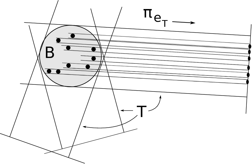
For a tube T=𝒟⁡([a,δ1/2)×[b,δ1/2))∈𝒯B′′T=\mathcal{D}([a,\delta^{1/2})\times[b,\delta^{1/2}))\in\mathcal{T}_{B}^{\prime\prime}, let eT∈S1e_{T}\in S^{1} for the unit vector perpendicular to line 𝒟⁡(a,b)⊂T\mathcal{D}(a,b)\subset T, and let EB:={eT:T∈𝒯B}E_{B}:=\{e_{T}:T\in\mathcal{T}_{B}\}. Then EBE_{B} is a (δ1/2,s)(\delta^{1/2},s)-set. Denote by πeT\pi_{e_{T}} the orthogonal projection onto the line spanned by eTe_{T}, see Figure 2.

Refer to caption
Figure 2. The tubes T∈𝒯B′′T\in\mathcal{T}_{B}^{\prime\prime}, and the projections πeT\pi_{e_{T}}.

Informally, the next lemma says that "for any B∈ℬB\in\mathcal{B}, in an overwhelming majority of directions eT∈EBe_{T}\in E_{B}, the set πeT​(PB)\pi_{e_{T}}(P_{B}), and all its reasonably large subsets, contain a (δ,s)(\delta,s)-set of nearly maximal cardinality, namely ≈δ−s/2\approx\delta^{-s/2}".

Lemma 4.19.

Let C0,C1,C2≥1C_{0},C_{1},C_{2}\geq 1 be constants. Then, if C2C_{2} is sufficiently large, depending on C0,C1C_{0},C_{1} and the various constants behind the ⪅\lessapprox-notation used above, there are at least (1−δC1​ϵ)​|𝒯B′′|(1-\delta^{C_{1}\epsilon})|\mathcal{T}_{B}^{\prime\prime}| "good" vectors eT∈EBe_{T}\in E_{B} with the following property: if PB′⊂PBP_{B}^{\prime}\subset P_{B} is a subset of cardinality |PB′|≥δC0​ϵ​|PB||P_{B}^{\prime}|\geq\delta^{C_{0}\epsilon}|P_{B}|, then πeT​(PB′)\pi_{e_{T}}(P_{B}^{\prime}) contains a (δ,s,C2)(\delta,s,C_{2})-set of cardinality ≥δC2​ϵ−s/2\geq\delta^{C_{2}\epsilon-s/2}.

Proof.

The proof is a variation of the standard "potential theoretic" argument, invented by Kaufman [12]; if the reader is not familiar with the technique, a similar but cleaner statement is Theorem 2 in [6]. First, observe that δ−1/2PB\delta^{-1/2}P_{B} is a (δ1/2,1)(\delta^{1/2},1)-set of cardinality ≈δ−1/2\approx\delta^{-1/2}. Next, consider the measures

μB:=1|PB|∑p∈δ−1/2PBχB⁡(p,δ1/2)δ\mu_{B}:=\frac{1}{|P_{B}|}\sum_{p\in\delta^{-1/2}P_{B}}\frac{\chi_{B(p,\delta^{1/2})}}{\delta}

and

ν:=1|EB|​∑e∈EBχB⁡(e,δ1/2)∩S1δ1/2,\nu:=\frac{1}{|E_{B}|}\sum_{e\in E_{B}}\frac{\chi_{B(e,\delta^{1/2})\cap S^{1}}}{\delta^{1/2}},

and note that μB​(ℝ2)∼1∼ν⁡(S1)\mu_{B}(\mathbb{R}^{2})\sim 1\sim\nu(S^{1}). For r≥δ1/2r\geq\delta^{1/2}, one has the uniform estimates μB​(B⁡(x,r))⪅r\mu_{B}(B(x,r))\lessapprox r and ν⁡(B⁡(e,r))⪅rs\nu(B(e,r))\lessapprox r^{s}, while for 0<r≤δ1/20<r\leq\delta^{1/2} one has the obvious improved estimates. After some straightforward computations, it follows that

(4.20) ∫S1Is​(πe​♯​μB)​𝑑ν​e:=∬[∫S1d​ν​e|πe​(x)−πe​(y)|s]​d​μB​x​d​μB​y⪅1.\int_{S^{1}}I_{s}(\pi_{e\sharp}\mu_{B})\,d\nu e:=\iint\left[\int_{S^{1}}\frac{d\nu e}{|\pi_{e}(x)-\pi_{e}(y)|^{s}}\right]\,d\mu_{B}x\,d\mu_{B}y\lessapprox 1.

Indeed, the inner integral (in brackets) can be estimated by ⪅1/|x−y|s\lessapprox 1/|x-y|^{s}, and then

∫S1Is​(πe​♯​μB)​𝑑ν​e⪅∫[∫d​μB​x|x−y|s]​d​μB​y⪅1,\int_{S^{1}}I_{s}(\pi_{e\sharp}\mu_{B})\,d\nu e\lessapprox\int\left[\int\frac{d\mu_{B}x}{|x-y|^{s}}\right]\,d\mu_{B}y\lessapprox 1,

since the inner integral is again bounded by ⪅1\lessapprox 1 for any y∈ℝ2y\in\mathbb{R}^{2}. Consequently, by Chebyshev’s inequality,

ν⁡({e∈S1:Is​(πe​♯​μB)≥δ−C​ϵ})⪅δC​ϵ,C≥1.\nu(\{e\in S^{1}:I_{s}(\pi_{e\sharp}\mu_{B})\geq\delta^{-C\epsilon}\})\lessapprox\delta^{C\epsilon},\quad C\geq 1.

Now, first, choose C2′≥1C_{2}^{\prime}\geq 1 so large that ν({e:Is(πe​♯μB})≥δ−C2′​ϵ})≤δC1​ϵν(S1)\nu(\{e:I_{s}(\pi_{e\sharp}\mu_{B}\})\geq\delta^{-C_{2}^{\prime}\epsilon}\})\leq\delta^{C_{1}\epsilon}\nu(S^{1}), and let E′:={e:Is​(πe​♯​μB)≤δ−C2′​ϵ}E^{\prime}:=\{e:I_{s}(\pi_{e\sharp}\mu_{B})\leq\delta^{-C_{2}^{\prime}\epsilon}\}. One evidently needs ≥(1−δC1​ϵ)​|EB|\geq(1-\delta^{C_{1}\epsilon})|E_{B}| arcs of the form B⁡(e,δ1/2)∩S1B(e,\delta^{1/2})\cap S^{1}, e∈EBe\in E_{B} to cover E′E^{\prime}, and this gives rise to a subset E⊂EBE\subset E_{B} with |E|≥(1−δC1​ϵ)​|EB||E|\geq(1-\delta^{C_{1}\epsilon})|E_{B}|. I claim that these are of desired "good" vectors.

For every e∈Ee\in E, by definition, there exists a vector e′∈B⁡(e,δ1/2)∩S1e^{\prime}\in B(e,\delta^{1/2})\cap S^{1} with

(4.21) ∬d​μ​x​d​μ​y|πe′​(x)−πe′​(y)|s=Is​(πe′​♯​μ)⪅δ−C2′​ϵ.\iint\frac{d\mu x\,d\mu y}{|\pi_{e^{\prime}}(x)-\pi_{e^{\prime}}(y)|^{s}}=I_{s}(\pi_{e^{\prime}\sharp}\mu)\lessapprox\delta^{-C_{2}^{\prime}\epsilon}.

Now, if PB′⊂PP_{B}^{\prime}\subset P is a subset of cardinality |PB′|≥δC0​ϵ​|PB||P_{B}^{\prime}|\geq\delta^{C_{0}\epsilon}|P_{B}| (as in the statement of the lemma), then the probability measure μ′\mu^{\prime}, defined in the obvious way by restricting and re-normalising μB\mu_{B} to the subset δ−1/2PB′\delta^{-1/2}P_{B}^{\prime}, still satisfies (4.21) with the ⪅\lessapprox-parameters depending on C0C_{0}. It follows that ℋ∞s​(πe′​(spt⁡μ′))⪆1\mathcal{H}^{s}_{\infty}(\pi_{e^{\prime}}(\operatorname{spt}\mu^{\prime}))\gtrapprox 1 (with similar dependence on C0C_{0}), and hence πe′​(spt⁡μ′)\pi_{e^{\prime}}(\operatorname{spt}\mu^{\prime}) contains a (δ1/2,s,C2)(\delta^{1/2},s,C_{2})-set of cardinality ≥δC2​ϵ−s/2\geq\delta^{C_{2}\epsilon-s/2} by Proposition 3.5, if C2≥1C_{2}\geq 1 is large enough (depending on C0C_{0} and C2′C_{2}^{\prime}, which just depends on C1C_{1}). Since πe′​(spt⁡μ′)\pi_{e^{\prime}}(\operatorname{spt}\mu^{\prime}) is contained in the δ1/2\delta^{1/2}-neighbourhood of πe′(δ−1/2PB′)\pi_{e^{\prime}}(\delta^{-1/2}P_{B}^{\prime}), the same conclusion holds for πe′(δ−1/2PB′)\pi_{e^{\prime}}(\delta^{-1/2}P_{B}^{\prime}). Finally, using |e′−e|≤δ1/2|e^{\prime}-e|\leq\delta^{1/2}, the conclusion remains valid for πe(δ−1/2PB′)\pi_{e}(\delta^{-1/2}P_{B}^{\prime}), and thus, rescaling by δ1/2\delta^{1/2}, the projection πe​(PB′)\pi_{e}(P_{B}^{\prime}) contains a (δ,s)(\delta,s)-set of cardinality ≥δC2​ϵ−s/2\geq\delta^{C_{2}\epsilon-s/2} for every e∈Ee\in E. ∎

Fix some constants C0,C1≥1C_{0},C_{1}\geq 1 and let C2C_{2} be specified by the lemma (the constant C0C_{0} will be fixed far below, wheres C1C_{1} will be specified momentarily). I define 𝒯B′⊂𝒯B′′\mathcal{T}_{B}^{\prime}\subset\mathcal{T}_{B}^{\prime\prime} by selecting the ≥(1−δC1​ϵ)​|𝒯B′′|\geq(1-\delta^{C_{1}\epsilon})|\mathcal{T}_{B}^{\prime\prime}| tubes indicated by the lemma. Then, if C1≥1C_{1}\geq 1 is large enough, (4.17) continues to hold for every q∈PBq\in P_{B}, and with 𝒯B′′\mathcal{T}_{B}^{\prime\prime} replaced by 𝒯B′\mathcal{T}_{B}^{\prime}:

(4.22) |𝒯B′∩𝒯δ1/2B(p)|≥|𝒯B′′∩𝒯δ1/2(p)|−δC1​ϵ|𝒯B′′|≈δ−s/2,p∈PB.|\mathcal{T}_{B}^{\prime}\cap\mathcal{T}_{\delta^{1/2}}^{B}(p)|\geq|\mathcal{T}_{B}^{\prime\prime}\cap\mathcal{T}_{\delta^{1/2}}(p)|-\delta^{C_{1}\epsilon}|\mathcal{T}_{B}^{\prime\prime}|\approx\delta^{-s/2},\quad p\in P_{B}.

Note that the parameters in the "≈\approx"-notation here do not depend on C1C_{1}, assuming that C1C_{1} is large enough. This completes the first refinement of 𝒯B′′\mathcal{T}_{B}^{\prime\prime}: roughly speaking, the conclusion was that "without loss of generality", the sets PBP_{B}, B∈ℬB\in\mathcal{B}, can be assumed to have large projections in every direction perpendicular to the tubes meeting BB. The second refinement (from 𝒯B′\mathcal{T}_{B}^{\prime} to 𝒯B\mathcal{T}_{B}) is concerned with the distribution of the balls B∈ℬB\in\mathcal{B} meeting a fixed δ1/2\delta^{1/2}-tube T∈𝒯δ1/2T\in\mathcal{T}_{\delta^{1/2}}. Roughly speaking, I claim that "without loss of generality", every tube T∈𝒯δ1/2T\in\mathcal{T}_{\delta^{1/2}} only meets a (1−s)(1-s)-dimensional family of balls B∈ℬB\in\mathcal{B}.

To formalise such thoughts, write

(4.23) Pδ1/2:={pB:B∈ℬ}.P_{\delta^{1/2}}:=\{p_{B}:B\in\mathcal{B}\}.

Since the balls B∈ℬB\in\mathcal{B} were assumed δ1/2\delta^{1/2}-separated (see (4.10)), it follows that Pδ1/2P_{\delta^{1/2}} is a (δ1/2,1)(\delta^{1/2},1)-set of cardinality |Pδ1/2|=|ℬ|≈δ−1/2|P_{\delta^{1/2}}|=|\mathcal{B}|\approx\delta^{-1/2}. Consider the following inequality (see explanations below):

(4.24) ∑T∈𝒯δ1/2∑B,B′∈ℬB≠B′χ𝒯B′∩𝒯B′′​(T)|pB−pB′|1−s=∑B,B′∈ℬB≠B′|𝒯B′∩𝒯B′′||pB−pB′|1−s⪅∑B,B′∈ℬB≠B′1|pB−pB′|⪅δ−1.\sum_{T\in\mathcal{T}_{\delta^{1/2}}}\mathop{\sum_{B,B^{\prime}\in\mathcal{B}}}_{B\neq B^{\prime}}\frac{\chi_{\mathcal{T}_{B}^{\prime}\cap\mathcal{T}_{B^{\prime}}^{\prime}}(T)}{|p_{B}-p_{B^{\prime}}|^{1-s}}=\mathop{\sum_{B,B^{\prime}\in\mathcal{B}}}_{B\neq B^{\prime}}\frac{|\mathcal{T}_{B}^{\prime}\cap\mathcal{T}_{B^{\prime}}^{\prime}|}{|p_{B}-p_{B^{\prime}}|^{1-s}}\lessapprox\mathop{\sum_{B,B^{\prime}\in\mathcal{B}}}_{B\neq B^{\prime}}\frac{1}{|p_{B}-p_{B^{\prime}}|}\lessapprox\delta^{-1}.

The first "⪅\lessapprox"-inequality uses the fact that 𝒯B′\mathcal{T}_{B}^{\prime} (or 𝒯B′′\mathcal{T}_{B^{\prime}}^{\prime}) is a (δ1/2,s)(\delta^{1/2},s)-set of tubes: since T∈𝒯B′∩𝒯B′′T\in\mathcal{T}_{B}^{\prime}\cap\mathcal{T}_{B^{\prime}}^{\prime} implies that pB,pB′∈Tp_{B},p_{B^{\prime}}\in T (recall (4.18)), this can only hold for ⪅1/|pB−pB′|s\lessapprox 1/|p_{B}-p_{B^{\prime}}|^{s} choices of T∈𝒯B′T\in\mathcal{T}_{B}^{\prime} (or T∈𝒯B′′T\in\mathcal{T}_{B^{\prime}}^{\prime}). The second "⪅\lessapprox"-inequality in (4.24) follows simply from the fact that Pδ1/2P_{\delta^{1/2}} is a (δ1/2,1)(\delta^{1/2},1)-set.

Fix a large constant C3≥1C_{3}\geq 1. It follows from (4.24) and Chebyshev’s inequality that

(4.25) ∑B,B′∈ℬB≠B′χ𝒯B′∩𝒯B′′​(T)|pB−pB′|1−s≥δ−C3​ϵ+s−1\mathop{\sum_{B,B^{\prime}\in\mathcal{B}}}_{B\neq B^{\prime}}\frac{\chi_{\mathcal{T}_{B}^{\prime}\cap\mathcal{T}_{B^{\prime}}^{\prime}}(T)}{|p_{B}-p_{B^{\prime}}|^{1-s}}\geq\delta^{-C_{3}\epsilon+s-1}

can only hold for ⪅δC3​ϵ−s\lessapprox\delta^{C_{3}\epsilon-s} tubes T∈𝒯δ1/2T\in\mathcal{T}_{\delta^{1/2}}. Recalling that |𝒯δ1/2|≈δ−s|\mathcal{T}_{\delta^{1/2}}|\approx\delta^{-s} by (4.14), this roughly says that the tubes satisfying (4.25) are exceptional. I need a the following slightly more accurate statement: for half of the balls B∈ℬB\in\mathcal{B}, only a tiny fraction of the tubes in T∈𝒯BT\in\mathcal{T}_{B} can satisfy (4.25), if C3≥1C_{3}\geq 1 was chosen large enough. Indeed, recall the constant C1C_{1} from the previous page and assume that, for a certain C3≥1C_{3}\geq 1, it holds that ≥δC1​ϵ​|𝒯B′|≈δC1​ϵ−s/2\geq\delta^{C_{1}\epsilon}|\mathcal{T}_{B}^{\prime}|\approx\delta^{C_{1}\epsilon-s/2} tubes in 𝒯B′\mathcal{T}_{B}^{\prime} satisfy (4.25) for B∈ℬ′⊂ℬB\in\mathcal{B}^{\prime}\subset\mathcal{B}, where |ℬ′|≥|ℬ|/2|\mathcal{B}^{\prime}|\geq|\mathcal{B}|/2. Then Lemma 4.1 applies at scale δ1/2\delta^{1/2}, and with the (δ1/2,1)(\delta^{1/2},1)-set ℬ′\mathcal{B}^{\prime}, and implies that the total number of tubes in 𝒯δ1/2\mathcal{T}_{\delta^{1/2}} satisfying (4.25) is ⪆δ−s\gtrapprox\delta^{-s}, where the implicit parameters depend on C1C_{1}, but clearly not on C3C_{3}. Comparing this with the upper bound ⪅δC3​ϵ−s\lessapprox\delta^{C_{3}\epsilon-s} gives an upper bound for C3C_{3}, which depends on C1C_{1}.

Hence, assuming that C3≥1C_{3}\geq 1 is large enough, the converse of (4.25) holds for all B∈ℬ′B\in\mathcal{B}^{\prime}, and for ≥(1−δC1​ϵ)​|𝒯B′|\geq(1-\delta^{C_{1}\epsilon})|\mathcal{T}_{B}^{\prime}| tubes in 𝒯B′\mathcal{T}_{B}^{\prime}. These tubes will be denoted by 𝒯B\mathcal{T}_{B}. And once more, if C1≥1C_{1}\geq 1 is large enough, the analogue of (4.22) continues to hold for 𝒯B\mathcal{T}_{B}:

(4.26) |𝒯B∩𝒯δ1/2B(p)|≈δ−s/2,p∈PB,B∈ℬ′.|\mathcal{T}_{B}\cap\mathcal{T}_{\delta^{1/2}}^{B}(p)|\approx\delta^{-s/2},\quad p\in P_{B},\>B\in\mathcal{B}^{\prime}.

Again, the parameters in the "≈\approx"-notation do not, in fact, depend on C1C_{1}, assuming that C1C_{1} is large enough. For each tube T∈𝒯BT\in\mathcal{T}_{B}, I further observe that the number MT:=|{B∈ℬ′:T∈𝒯B}|M_{T}:=|\{B\in\mathcal{B}^{\prime}:T\in\mathcal{T}_{B}\}| satisfies

(4.27) MT⪅δ(s−1)/2,M_{T}\lessapprox\delta^{(s-1)/2},

where the implicit constants depend on C3C_{3}. Indeed, the failure of (4.27) (say: MT≥δ−(2C3ϵ+s−1)/2M_{T}\geq\delta^{-(2C_{3}\epsilon+s-1)/2}) would imply that there are far more than δs−1\delta^{s-1} pairs B,B′∈ℬ′⊂ℬB,B^{\prime}\in\mathcal{B}^{\prime}\subset\mathcal{B} such that T∈𝒯B∩𝒯B′⊂𝒯B′∩𝒯B′′T\in\mathcal{T}_{B}\cap\mathcal{T}_{B^{\prime}}\subset\mathcal{T}_{B}^{\prime}\cap\mathcal{T}_{B^{\prime}}^{\prime}, which would violate (4.25) (since |pB−pB′|≲1|p_{B}-p_{B^{\prime}}|\lesssim 1 for all pairs B,B′∈ℬB,B^{\prime}\in\mathcal{B}).

4.4. Considerations at scale δ\delta

From now on, only the points in PBP_{B}, B∈ℬ′B\in\mathcal{B}^{\prime}, play any role in the proof. Set

P′:=⋃B∈ℬ′PB,P^{\prime}:=\bigcup_{B\in\mathcal{B}^{\prime}}P_{B},

which is a (δ,1)(\delta,1)-set of cardinality ≈δ−1\approx\delta^{-1}, since |ℬ′|≈δ−1/2|\mathcal{B}^{\prime}|\approx\delta^{-1/2} and |PB|≈δ−1/2|P_{B}|\approx\delta^{-1/2} for B∈ℬB\in\mathcal{B} by the definition of PBP_{B} (just above (4.16)). Fix p∈P′p\in P^{\prime} and B∈ℬ′B\in\mathcal{B}^{\prime} such that p∈PBp\in P_{B}. For every

T∈𝒯B∩𝒯δ1/2B​(p),T\in\mathcal{T}_{B}\cap\mathcal{T}^{B}_{\delta^{1/2}}(p),

define 𝒯p′\mathcal{T}_{p}^{\prime} to consist of all the δ\delta-tubes 𝒯p\mathcal{T}_{p}, which are δ\delta-children of TT. By definition of 𝒯δ1/2B​(p)\mathcal{T}_{\delta^{1/2}}^{B}(p) (see (4.15)) and (4.26)), the resulting subset 𝒯p′⊂𝒯p\mathcal{T}_{p}^{\prime}\subset\mathcal{T}_{p} is a (δ,s)(\delta,s)-set of tubes containing pp, and with

(4.28) |𝒯p′|≈δ−s.|\mathcal{T}_{p}^{\prime}|\approx\delta^{-s}.

Thus, the set P′⊂PP^{\prime}\subset P and the families 𝒯p′⊂𝒯p\mathcal{T}_{p}^{\prime}\subset\mathcal{T}_{p}, p∈P′p\in P^{\prime}, satisfy precisely the same hypotheses as the original families PP and 𝒯p\mathcal{T}_{p} in Theorem 4.3. So, for notational, convenience, I re-define P:=P′P:=P^{\prime}, 𝒯p:=𝒯p′\mathcal{T}_{p}:=\mathcal{T}_{p}^{\prime}, and ℬ:=ℬ′\mathcal{B}:=\mathcal{B}^{\prime}. As before (in Remark 4.6), I continue to assume, without loss of generality, that

𝒯:=⋃p∈P𝒯p.\mathcal{T}:=\bigcup_{p\in P}\mathcal{T}_{p}.

I also re-define 𝒯δ1/2\mathcal{T}_{\delta^{1/2}} to be the union of the families 𝒯B\mathcal{T}_{B}, B∈ℬB\in\mathcal{B}. Note that, with this definition of 𝒯δ1/2\mathcal{T}_{\delta^{1/2}}, one has (4.27) for all tubes in 𝒯δ1/2\mathcal{T}_{\delta^{1/2}}.

Compared with the original families 𝒯p\mathcal{T}_{p}, the new families 𝒯p\mathcal{T}_{p} now enjoy additional regularity properties, which will be useful during the remainder of the proof. To exploit these, I record the following observation:

Lemma 4.29.

Assume that p∈B∈ℬp\in B\in\mathcal{B} and T∈𝒯pT\in\mathcal{T}_{p}. Then the δ1/2\delta^{1/2}-parent of TT belongs to 𝒯B\mathcal{T}_{B}. In particular, the δ1/2\delta^{1/2}-parents of the tubes in 𝒯\mathcal{T} belong to 𝒯δ1/2\mathcal{T}_{\delta^{1/2}}.

Proof.

This follows immediately from the construction of 𝒯p′\mathcal{T}_{p}^{\prime} – which is now called 𝒯p\mathcal{T}_{p}. ∎

For T∈𝒯T\in\mathcal{T}, write

NT:=|{p∈P:T∈𝒯p}|,N_{T}:=|\{p\in P:T\in\mathcal{T}_{p}\}|,

which is the analogue of the number MTM_{T} at scale δ\delta. I make the following (rather familiar) claim: for at least half of the points p∈Pp\in P, only a tiny fraction of the tubes in 𝒯p\mathcal{T}_{p} can fail to satisfy NT⪅δs−1N_{T}\lessapprox\delta^{s-1}. The proof is virtually the same as for the numbers MTM_{T}. One starts with the inequality

∑T∈𝒯∑p,q∈Pp≠qχ𝒯p∩𝒯q​(T)|p−q|1−s⪅δ−2,\sum_{T\in\mathcal{T}}\mathop{\sum_{p,q\in P}}_{p\neq q}\frac{\chi_{\mathcal{T}_{p}\cap\mathcal{T}_{q}}(T)}{|p-q|^{1-s}}\lessapprox\delta^{-2},

which is analogous to and proven in the same way as (4.24). Thus, only ⪅δC4​ϵ−2​s\lessapprox\delta^{C_{4}\epsilon-2s} tubes in 𝒯p\mathcal{T}_{p} can satisfy

∑p,q∈Pp≠qχ𝒯p∩𝒯q​(T)|p−q|1−s≥δ−C4​ϵ+2​s−2.\mathop{\sum_{p,q\in P}}_{p\neq q}\frac{\chi_{\mathcal{T}_{p}\cap\mathcal{T}_{q}}(T)}{|p-q|^{1-s}}\geq\delta^{-C_{4}\epsilon+2s-2}.

Hence, using Lemma 4.1 as before, the inequality above can only hold for a tiny fraction (depending on C4C_{4}) of the tubes in 𝒯p\mathcal{T}_{p}, for half of the points in PP. This implies the statement about the numbers NTN_{T}. Now, as final refinement, I only keep the "good" half of the points in PP, and for those p∈Pp\in P, I re-define 𝒯p\mathcal{T}_{p} to consist of the tubes TT with

(4.30) NT⪅δs−1.N_{T}\lessapprox\delta^{s-1}.

If C4C_{4} was large enough, the cardinality estimate (4.28) stays valid. Finally, if 𝒯\mathcal{T} is re-defined as the union of the (remaining) tubes in 𝒯p\mathcal{T}_{p}, p∈Pp\in P, one may assume that (4.30) holds uniformly for all T∈𝒯T\in\mathcal{T}.

Fix p∈Pp\in P and T∈𝒯T\in\mathcal{T}. Recall that the pair (p,T)(p,T) is called an incidence, if T∈𝒯pT\in\mathcal{T}_{p}, and the collection of all incidences is denoted by I⁡(P,𝒯):={(p,T):T∈𝒯p}I(P,\mathcal{T}):=\{(p,T):T\in\mathcal{T}_{p}\}. Evidently

(4.31) |I⁡(P,𝒯)|=∑p∈P|𝒯p|≈δ−s−1.|I(P,\mathcal{T})|=\sum_{p\in P}|\mathcal{T}_{p}|\approx\delta^{-s-1}.

By the uniform upper bound (4.30), any tube T∈𝒯T\in\mathcal{T} can only be incident to ⪅δs−1\lessapprox\delta^{s-1} points in PP. Since |𝒯|⪅δ−2​s|\mathcal{T}|\lessapprox\delta^{-2s} by the main counter assumption (4.8), the estimate (4.31) shows that there exist ≈δ−2​s\approx\delta^{-2s} tubes in 𝒯\mathcal{T} with NT≈δs−1N_{T}\approx\delta^{s-1}. These tubes will be called good tubes, and they will be denoted by 𝒯G\mathcal{T}^{G}.

Lemma 4.32.

Any fixed tube T0∈𝒯δ1/2T_{0}\in\mathcal{T}_{\delta^{1/2}} can only have ⪅δ−s\lessapprox\delta^{-s} children in 𝒯G\mathcal{T}^{G}.

Proof.

Write 𝒯G​(T0):={T∈𝒯G:T⊂T0}\mathcal{T}^{G}(T_{0}):=\{T\in\mathcal{T}^{G}:T\subset T_{0}\}, and let IG​(T0)I^{G}(T_{0}) be the set of incidences

IG​(T0):={(p,T)∈P×𝒯:T∈𝒯p∩𝒯G​(T0)}.I^{G}(T_{0}):=\{(p,T)\in P\times\mathcal{T}:T\in\mathcal{T}_{p}\cap\mathcal{T}^{G}(T_{0})\}.

By the definition of good tubes, evidently

|IG​(T0)|⪆|𝒯G​(T0)|​δs−1.|I^{G}(T_{0})|\gtrapprox|\mathcal{T}^{G}(T_{0})|\delta^{s-1}.

On the other hand, by Lemma 4.29, an incidence (p,T)∈P×𝒯p(p,T)\in P\times\mathcal{T}_{p} can only occur, if the δ1/2\delta^{1/2}-parent of TT belongs to 𝒯Bp\mathcal{T}_{B_{p}} for the (unique) ball Bp∈ℬB_{p}\in\mathcal{B} containing pp. For T⊂T0T\subset T_{0}, the δ1/2\delta^{1/2}-parent is evidently T0T_{0}, so

T⊂T0​ and ​(p,T)∈𝒯p⟹T0∈𝒯Bp.T\subset T_{0}\text{ and }(p,T)\in\mathcal{T}_{p}\quad\Longrightarrow\quad T_{0}\in\mathcal{T}_{B_{p}}.

Now, recall from the estimate MT0⪅δ(s−1)/2M_{T_{0}}\lessapprox\delta^{(s-1)/2} (see (4.27)), that there are only ⪅δ(s−1)/2\lessapprox\delta^{(s-1)/2} balls BB with T0∈𝒯BT_{0}\in\mathcal{T}_{B}. For every such a ball BB, every point p∈PBp\in P_{B} can be incident to ⪅δ−s/2\lessapprox\delta^{-s/2} tubes T∈𝒯pT\in\mathcal{T}_{p} with T⊂T0T\subset T_{0} (for the simple reason that T0T_{0} only contains ⪅δ−s/2\lessapprox\delta^{-s/2} tubes in 𝒯p\mathcal{T}_{p} by Lemma 3.16). Recalling that |PB|⪅δ−1/2|P_{B}|\lessapprox\delta^{-1/2}, this gives the upper bound

(4.33) |IG(T0)|≤∑B:T0∈𝒯B|{(p,T)∈B×𝒯:T∈𝒯p∩𝒯G(T0)}|⪅δ(s−1)/2⋅δ−1/2⋅δ−s/2=δ−1.|I^{G}(T_{0})|\leq\sum_{B:T_{0}\in\mathcal{T}_{B}}|\{(p,T)\in B\times\mathcal{T}:T\in\mathcal{T}_{p}\cap\mathcal{T}^{G}(T_{0})\}|\lessapprox\delta^{(s-1)/2}\cdot\delta^{-1/2}\cdot\delta^{-s/2}=\delta^{-1}.

Comparing with the lower bound for |IG​(T0)||I^{G}(T_{0})| completes the proof. ∎

To sum up the most recent observations, there are ≈δ−2​s\approx\delta^{-2s} good tubes, each one of which is contained in some tube of 𝒯δ1/2\mathcal{T}_{\delta^{1/2}}, and each tube in 𝒯δ1/2\mathcal{T}_{\delta^{1/2}} can only contain ⪅δ−s\lessapprox\delta^{-s} good tubes. By the main counter assumption (4.8), moreover, one has |𝒯δ1/2|⪅δ−s|\mathcal{T}_{\delta^{1/2}}|\lessapprox\delta^{-s}, which finally implies that there exists a tube T0∈𝒯T_{0}\in\mathcal{T} with |𝒯G​(T0)|≈δ−s|\mathcal{T}^{G}(T_{0})|\approx\delta^{-s}. For simplicity, write

(4.34) 𝒯0:=𝒯G​(T0).\mathcal{T}_{0}:=\mathcal{T}^{G}(T_{0}).

I now claim that there are ≈δ(s−1)/2\approx\delta^{(s-1)/2} balls B∈ℬB\in\mathcal{B}, say ℬ0\mathcal{B}_{0}, such that T0∈𝒯BT_{0}\in\mathcal{T}_{B} for B∈ℬ0B\in\mathcal{B}_{0}, and such that in each ball B∈ℬ0B\in\mathcal{B}_{0} one finds ≈δ−1/2\approx\delta^{-1/2} points of PBP_{B}, say PB′P_{B}^{\prime}, with a near-maximal number of incidences with 𝒯0\mathcal{T}_{0}, namely

(4.35) |𝒯p∩𝒯0|≈δ−s/2,p∈PB′,B∈ℬ0.|\mathcal{T}_{p}\cap\mathcal{T}_{0}|\approx\delta^{-s/2},\qquad p\in P_{B}^{\prime},\>B\in\mathcal{B}_{0}.

This follows directly from the proof of Lemma 4.32. First observe that |IG​(T0)|≈δ−1|I^{G}(T_{0})|\approx\delta^{-1}, since |𝒯0|≈δ−s|\mathcal{T}_{0}|\approx\delta^{-s}. Next, have a look at the upper bound (4.33), and observe that if any part of the claim failed, the bound would be lower than δ−1\delta^{-1}. This establishes the claim.

Now, since T0∈𝒯δ1/2T_{0}\in\mathcal{T}_{\delta^{1/2}}, the converse of (4.25) holds for T0T_{0} (recall the definition of 𝒯B\mathcal{T}_{B} next to (4.26), and recall that every tube in 𝒯δ1/2\mathcal{T}_{\delta^{1/2}} belongs to 𝒯B\mathcal{T}_{B} for some BB):

∑B,B∈ℬ0B≠B′1|pB−pB′|1−s⪅δs−1.\mathop{\sum_{B,B\in\mathcal{B}_{0}}}_{B\neq B^{\prime}}\frac{1}{|p_{B}-p_{B^{\prime}}|^{1-s}}\lessapprox\delta^{s-1}.

Using Chebyshev’s inequality, this implies that a further subset ℬ0′⊂ℬ0\mathcal{B}_{0}^{\prime}\subset\mathcal{B}_{0} of cardinality |ℬ0′|≈δ(s−1)/2|\mathcal{B}_{0}^{\prime}|\approx\delta^{(s-1)/2} satisfies

∑B′∈ℬ01|pB−pB′|1−s⪅δ(s−1)/2,B∈ℬ0′.\sum_{B^{\prime}\in\mathcal{B}_{0}}\frac{1}{|p_{B}-p_{B}^{\prime}|^{1-s}}\lessapprox\delta^{(s-1)/2},\quad B\in\mathcal{B}_{0}^{\prime}.

and then ℬ0′\mathcal{B}_{0}^{\prime} is a (δ1/2,1−s)(\delta^{1/2},1-s)-set of cardinality ≈δ(s−1)/2\approx\delta^{(s-1)/2}. Since the balls ℬ0′\mathcal{B}_{0}^{\prime} satisfy precisely the same estimates as ℬ0\mathcal{B}_{0}, I will continue writing ℬ0:=ℬ0′\mathcal{B}_{0}:=\mathcal{B}_{0}^{\prime}. For convenience, assume that T0T_{0} is a vertical tube (that is, change coordinates so that this holds). Then the yy-coordinates of the points pB∈Bp_{B}\in B, B∈ℬ0B\in\mathcal{B}_{0}, form a (δ1/2,1−s)(\delta^{1/2},1-s)-set in [−1,1][-1,1]. Denote these yy-coordinates by A1:={pByA_{1}:=\{p_{B}^{y}, B∈ℬ0}B\in\mathcal{B}_{0}\}.

4.5. Quasi-product sets, and concluding the proof of Theorem 4.3

Now, recall (from above (4.35)) the subsets PB′⊂PBP_{B}^{\prime}\subset P_{B}, defined for B∈ℬ0B\in\mathcal{B}_{0}. They have cardinality |PB′|≥δC0​ϵ​|PB||P_{B}^{\prime}|\geq\delta^{C_{0}\epsilon}|P_{B}| for some constant C0≥1C_{0}\geq 1. This is the constant with which one wants to apply Lemma 4.19: since T0∈𝒯B′T_{0}\in\mathcal{T}_{B}^{\prime} (recall (4.22)), the projection of π⁡(PB′)\pi(P_{B}^{\prime}) of PB′P_{B}^{\prime} to the xx-axis contains a (δ,s)(\delta,s)-set ΔB\Delta_{B} of cardinality |ΔB|≥δC2​ϵ−s/2|\Delta_{B}|\geq\delta^{C_{2}\epsilon-s/2}.

Consider the "quasi-product set"

F′:=⋃pBy∈A1ΔB×{pBy}.F^{\prime}:=\bigcup_{p_{B}^{y}\in A_{1}}\Delta_{B}\times\{p_{B}^{y}\}.

Fix (a,b)=(a,pBy)∈F′(a,b)=(a,p_{B}^{y})\in F^{\prime}, B∈ℬ0B\in\mathcal{B}_{0}. Then a=π⁡(p)a=\pi(p) for some p=p(a,b)∈PB′p=p_{(a,b)}\in P_{B}^{\prime}, so that |(a,b)−p|≤2​δ1/2|(a,b)-p|\leq 2\delta^{1/2}. Recall that (4.35) holds for pp, and let T∈𝒯p∩𝒯0T\in\mathcal{T}_{p}\cap\mathcal{T}_{0}. By elementary geometry, using |(a,b)−p|≤2​δ1/2|(a,b)-p|\leq 2\delta^{1/2} and p∈T⊂T0p\in T\subset T_{0}, the point (a,b)∈F′(a,b)\in F^{\prime} is covered by B⁡(0,10)∩T′B(0,10)\cap T^{\prime} for some dyadic δ\delta-tube T′T^{\prime} in the C​δC\delta-neighbourhood of TT. (By this, I mean that if T=𝒟⁡(Q)T=\mathcal{D}(Q), then T′=𝒟⁡(Q′)T^{\prime}=\mathcal{D}(Q^{\prime}) for some dyadic δ\delta-square Q′Q^{\prime} with dist⁡(Q,Q′)≤C​δ\operatorname{dist}(Q,Q^{\prime})\leq C\delta.) This is best explained by a picture, see Figure 3.
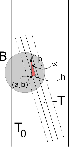
Refer to caption
Figure 3. The geometry of the tubes T0,TT_{0},T and the points (a,b)(a,b) and p=p(a,b)p=p_{(a,b)}. Since T⊂T0T\subset T_{0}, the angle α\alpha is ≲δ1/2\lesssim\delta^{1/2}. Since p,(a,b)∈Bp,(a,b)\in B, the distance between the points pp and (a,b)(a,b) is no greater than 2​δ1/22\delta^{1/2}. Hence h≲δh\lesssim\delta, which ensures that (a,b)(a,b) is contained in B⁡(0,10)∩T′B(0,10)\cap T^{\prime} for some dyadic δ\delta-tube T′T^{\prime} parallel to, and at distance ≲δ\lesssim\delta, from T∈𝒯pT\in\mathcal{T}_{p}.

Now, for each T∈𝒯0T\in\mathcal{T}_{0}, choose an ordinary C​δC\delta-tube parallel to TT, which covers B⁡(0,10)∩T′B(0,10)\cap T^{\prime} for all the dyadic δ\delta-tubes T′T^{\prime} in the C​δC\delta-neighbourhood of TT. The collection of all ordinary C​δC\delta-tubes so obtained is denoted by 𝒯o\mathcal{T}^{o} (here "oo" stands for "ordinary"). Then

|𝒯o|∼|𝒯0|≈δ−s.|\mathcal{T}^{o}|\sim|\mathcal{T}_{0}|\approx\delta^{-s}.

In particular, 𝒯o\mathcal{T}^{o} contains the ordinary C​δC\delta-tubes produced from the dyadic δ\delta-tubes in 𝒯p(a,b)∩𝒯0\mathcal{T}_{p_{(a,b)}}\cap\mathcal{T}_{0}. By (4.35) and the discussion above, this gives rise to a (δ,s)(\delta,s)-subset 𝒯(a,b)o⊂𝒯o\mathcal{T}^{o}_{(a,b)}\subset\mathcal{T}^{o} of ordinary C​δC\delta-tubes of cardinality |𝒯o(a,b)|≈δ−s/2|\mathcal{T}^{o}_{(a,b)}|\approx\delta^{-s/2}, with the property that

(a,b)∈T,T∈𝒯(a,b)o.(a,b)\in T,\qquad T\in\mathcal{T}^{o}_{(a,b)}.

Finally, consider the following affine transformation of F′F^{\prime}:

F:=⋃b∈A1Ab×{b},F:=\bigcup_{b\in A_{1}}A_{b}\times\{b\},

where Ab:=δ−1/2ΔBA_{b}:=\delta^{-1/2}\Delta_{B}. Note that each AbA_{b} is a (δ1/2,s)(\delta^{1/2},s)-set, and recall that A1A_{1} is a (δ1/2,1−s)(\delta^{1/2},1-s)-set. Clearly F=Aff⁡(F′)F=\operatorname{Aff}(F^{\prime}), where Aff(x,y)=(δ−1/2x,y)\operatorname{Aff}(x,y)=(\delta^{-1/2}x,y). Then 𝒯′:=Aff⁡(𝒯o)={Aff⁡(T):T∈𝒯o}\mathcal{T}^{\prime}:=\operatorname{Aff}(\mathcal{T}^{o})=\{\operatorname{Aff}(T):T\in\mathcal{T}^{o}\} is a family of ordinary C′​δ1/2C^{\prime}\delta^{1/2}-tubes of cardinality |𝒯′|∼|𝒯|≈δ−s|\mathcal{T}^{\prime}|\sim|\mathcal{T}|\approx\delta^{-s}. Moreover, every point x=(δ−1/2a,b)∈Fx=(\delta^{-1/2}a,b)\in F is is contained in a (δ1/2,s)(\delta^{1/2},s)-subset 𝒯x′⊂𝒯′\mathcal{T}_{x}^{\prime}\subset\mathcal{T}^{\prime} of ordinary C′​δ1/2C^{\prime}\delta^{1/2}-tubes with |𝒯x′|≈δ−s/2|\mathcal{T}_{x}^{\prime}|\approx\delta^{-s/2}, namely 𝒯x′:=Aff⁡(𝒯(a,b)o)\mathcal{T}_{x}^{\prime}:=\operatorname{Aff}(\mathcal{T}_{(a,b)}^{o}). The existence of FF and the families 𝒯′,𝒯x′\mathcal{T}^{\prime},\mathcal{T}_{x}^{\prime}, now contradict the next proposition (at scale δ1/2\delta^{1/2}, with P=FP=F, 𝒯=𝒯′\mathcal{T}=\mathcal{T}^{\prime} and τ=1−s>0\tau=1-s>0). This completes the proof of Theorem 4.3.

4.6. An incidence theorem for quasi-product sets

The wording "quasi-product set" is rather informal, and simply refers to sets PP of the form (4.37) below (if all the sets AbA_{b} were the same, then PP would truly be a product set). On the last meters of the proof above, such a set, namely FF, was constructed: it turned out that the points x∈Fx\in F were each incident to a large family 𝒯x′\mathcal{T}_{x}^{\prime} of not-too-concentrated tubes, and all the families 𝒯x′\mathcal{T}_{x}^{\prime} were subsets of a fixed small family 𝒯′\mathcal{T}^{\prime}. The next, and final, proposition shows that this is simply not possible.

Proposition 4.36.

Given 0<s<10<s<1 and τ>0\tau>0, there exists a number ϵ=ϵ⁡(s,τ)>0\epsilon=\epsilon(s,\tau)>0 such that the following holds. Let B⊂[0,1]B\subset[0,1] be a (δ,τ,δ−ϵ)(\delta,\tau,\delta^{-\epsilon})-set of cardinality |B|≳δ−τ+ϵ|B|\gtrsim\delta^{-\tau+\epsilon}, and for each b∈Bb\in B, assume that Ab⊂[0,1]A_{b}\subset[0,1] is a (δ,s,δ−ϵ)(\delta,s,\delta^{-\epsilon})-set of cardinality |Ab|≳δ−s+ϵ|A_{b}|\gtrsim\delta^{-s+\epsilon}. Consider the (δ,s+τ,δ−2​ϵ)(\delta,s+\tau,\delta^{-2\epsilon})-set

(4.37) P:=⋃b∈BAb×{b}.P:=\bigcup_{b\in B}A_{b}\times\{b\}.

Assume that 𝒯\mathcal{T} is a collection of (ordinary) δ\delta-tubes such every family {T∈𝒯:p∈T}\{T\in\mathcal{T}:p\in T\}, p∈Pp\in P, contains in a (δ,s,δ−ϵ)(\delta,s,\delta^{-\epsilon})-set 𝒯p⊂𝒯\mathcal{T}_{p}\subset\mathcal{T} with |𝒯p|≳δ−s+ϵ|\mathcal{T}_{p}|\gtrsim\delta^{-s+\epsilon}. Then |𝒯|≳δ−2​s−ϵ|\mathcal{T}|\gtrsim\delta^{-2s-\epsilon}.

The proof of Proposition 4.36 is, again, based on a counter assumption, namely |𝒯|≤δ−2​s−ϵ|\mathcal{T}|\leq\delta^{-2s-\epsilon}. For the remainder of the paper, the notations ⪅\lessapprox, ⪆\gtrapprox and ≈\approx, and the concept of (δ,t)(\delta,t)-set, are defined exactly as before, in Section 4.1, but now relative to the "ϵ\epsilon" in this counter assumption. Naturally, the implicit constants C,CϵC,C_{\epsilon} are now also allowed to depend on τ\tau, in addition to ss.

Before starting the proof of Proposition 4.36 in earnest, I recall two standard results from additive combinatorics. The first is the Balog-Szemerédi-Gowers theorem. The statement below is taken verbatim from p. 196 in [2]. For a proof, see [21], p. 267.

Theorem 4.38 (Balog-Szemerédi-Gowers).

There exists an absolute constant C≥1C\geq 1 such that the following holds. Let A,B⊂ℝA,B\subset\mathbb{R} be finite sets, and assume that G⊂A×BG\subset A\times B is a set of pairs such that

|G|≥|A|​|B|Kand|{x+y:(x,y)∈G}|≤K​|A|1/2​|B|1/2|G|\geq\frac{|A||B|}{K}\quad\text{and}\quad|\{x+y:(x,y)\in G\}|\leq K|A|^{1/2}|B|^{1/2}

for some K>1K>1. Then, there exist A′⊂AA^{\prime}\subset A and B′⊂BB^{\prime}\subset B satisfying

  • •

    |A′|≥K−C​|A||A^{\prime}|\geq K^{-C}|A|, |B′|≥K−C​|B||B^{\prime}|\geq K^{-C}|B|,

  • •

    |A′+B′|≤KC​|A|1/2​|B|1/2|A^{\prime}+B^{\prime}|\leq K^{C}|A|^{1/2}|B|^{1/2}, and

  • •

    |G∩(A′×B′)|≥K−C​|A|​|B||G\cap(A^{\prime}\times B^{\prime})|\geq K^{-C}|A||B|.

The second auxiliary result is the Plünnecke-Ruzsa inequality, whose proof can also be found in [21]:

Theorem 4.39 (Plünnecke-Ruzsa).

Assume that A,B⊂ℝA,B\subset\mathbb{R} are finite sets such that

|A+B|≤C​|A||A+B|\leq C|A|

for some integer C≥1C\geq 1. Then

|Bm±Bn|≤Cm+n​|A||B^{m}\pm B^{n}|\leq C^{m+n}|A|

for all m,n∈ℕm,n\in\mathbb{N}.

Remark 4.40.

Theorem 4.39 will be applied in the following form: if A,B⊂ℝA,B\subset\mathbb{R} are δ\delta-separated sets with |A|≈|B||A|\approx|B| and

N⁡(A+B,δ)⪅|A|,N(A+B,\delta)\lessapprox|A|,

then N⁡(B+B,δ)⪅|A|N(B+B,\delta)\lessapprox|A|. This statement follows easily from Theorem 4.39 by considering the sets [A]δ={[a]δ:a∈A}⊂δ​ℤ[A]_{\delta}=\{[a]_{\delta}:a\in A\}\subset\delta\mathbb{Z} and [B]δ:={[b]δ;b∈B}⊂δ​ℤ[B]_{\delta}:=\{[b]_{\delta};b\in B\}\subset\delta\mathbb{Z}, where [x]δ∈δ​ℤ[x]_{\delta}\in\delta\mathbb{Z} stands for the largest number δ​n∈δ​ℤ\delta n\in\delta\mathbb{Z} satisfying δ​n≤x\delta n\leq x. Then the hypothesis N⁡(A+B,δ)⪅|A|N(A+B,\delta)\lessapprox|A| implies that |[A]δ+[B]δ|⪅|[A]|δ|[A]_{\delta}+[B]_{\delta}|\lessapprox|[A]|_{\delta}, so Theorem 4.39 can be applied.

Proof of Proposition 4.36.

I start by making three convenient extra assumptions, which are not difficult to arrange. First, every tube in 𝒯\mathcal{T} meets only one point in each set Ab×{b}A_{b}\times\{b\} (that is, the tubes in 𝒯\mathcal{T} are "roughly vertical"); this can be arranged by restricting attention to those tubes in each 𝒯p\mathcal{T}_{p}, which form an angle ⪆1\gtrapprox 1 with horizontal lines. By the (δ,s)(\delta,s)-set hypothesis, ≈δ−s\approx\delta^{-s} tubes remain in each 𝒯p\mathcal{T}_{p}, and then one can re-define 𝒯\mathcal{T} as the union of the reduced families 𝒯p\mathcal{T}_{p}. In particular, now each tube in 𝒯\mathcal{T} only intersects the lines ℝ×{b}\mathbb{R}\times\{b\}, b∈Bb\in B, inside a single interval of length ⪅δ\lessapprox\delta. After this procedure, one can remove some points from each Ab×{b}A_{b}\times\{b\} so that the mutual separation exceeds the length of the intervals mentioned above; again, by the (δ,s)(\delta,s)-set hypothesis, this can be arranged to that ≈δ−s\approx\delta^{-s} points remain for every bb.

Second,

Ab⊂δ​ℤ,b∈B.A_{b}\subset\delta\mathbb{Z},\qquad b\in B.

This can be arranged by perturbing the points of AbA_{b} by ≤δ\leq\delta. The tubes in 𝒯p\mathcal{T}_{p} may no longer contain pp, but the 100​δ100\delta-neighbourhoods of the tubes in 𝒯p\mathcal{T}_{p} certainly do. These neighbourhoods can be covered by 200200 ordinary δ\delta-tubes, each, which gives rise to a new family 𝒯′\mathcal{T}^{\prime} of ordinary δ\delta-tubes with |𝒯′|∼|𝒯||\mathcal{T}^{\prime}|\sim|\mathcal{T}|. Then, one can prove the proposition for 𝒯′\mathcal{T}^{\prime} instead of 𝒯\mathcal{T}.

Third, if b1,b2,b3∈Bb_{1},b_{2},b_{3}\in B, and T,T′∈𝒯T,T^{\prime}\in\mathcal{T} are two tubes both containing certain points (a1,b1)∈Ab1×{b1}(a_{1},b_{1})\in A_{b_{1}}\times\{b_{1}\} and (a3,b3)∈Ab3×{b3}(a_{3},b_{3})\in A_{b_{3}}\times\{b_{3}\}, then T∪T′T\cup T^{\prime} can only contain one point in Ab2×{b2}A_{b_{2}}\times\{b_{2}\}. This is similar to the first reduction: it follows from the assumption T∪T′T\cup T^{\prime} intersects ℝ×{b2}\mathbb{R}\times\{b_{2}\} inside a single interval of length ⪅δ\lessapprox\delta (since T∪T′T\cup T^{\prime} is contained in the δ\delta-neighbourhood of the line connecting (a1,b1)(a_{1},b_{1}) to (a3,b3)(a_{3},b_{3}), and both tubes were already assumed to be roughly vertical). Thus, if the separation of Ab2A_{b_{2}} exceeds the length of any such interval, the claim is true. And this can, as before, be arranged by discarding a few points from A2A_{2}.

The proof starts in earnest now, and I make the counter assumption |𝒯|≤δ−2​s−ϵ|\mathcal{T}|\leq\delta^{-2s-\epsilon}, or, in short,

(4.41) |𝒯|⪅δ−2​s.|\mathcal{T}|\lessapprox\delta^{-2s}.

For T∈𝒯T\in\mathcal{T}, write

NT:=|{p∈P:T∈𝒯p}|.N_{T}:=|\{p\in P:T\in\mathcal{T}_{p}\}|.

Then, by the first "convenient extra assumption" above, one has the uniform bound

(4.42) NT≤|B|⪅δ−τ.N_{T}\leq|B|\lessapprox\delta^{-\tau}.

On the other hand

∑T∈𝒯NT=∑p∈P|𝒯p|⪆|P|​δ−s=δ−2​s−τ.\sum_{T\in\mathcal{T}}N_{T}=\sum_{p\in P}|\mathcal{T}_{p}|\gtrapprox|P|\delta^{-s}=\delta^{-2s-\tau}.

By the counter assumption (4.41), one sees that NT≈δ−τN_{T}\approx\delta^{-\tau} for ≈δ−2​s\approx\delta^{-2s} tubes in 𝒯\mathcal{T}. Consequently,

(4.43) ∑T∈𝒯|{(p,q)∈P×P:p∼Tq}|⪆δ−2​s−2​τ,\sum_{T\in\mathcal{T}}|\{(p,q)\in P\times P:p\sim_{T}q\}|\gtrapprox\delta^{-2s-2\tau},

where p∼Tqp\sim_{T}q, if and only if p≠qp\neq q and T∈𝒯p∩𝒯qT\in\mathcal{T}_{p}\cap\mathcal{T}_{q}. Write p∼qp\sim q, if p∼Tqp\sim_{T}q for some T∈𝒯T\in\mathcal{T}, and Q:={(p,q):p∼q}Q:=\{(p,q):p\sim q\}. Then the left hand side of the inequality above can be re-written and estimated as

∑p∼q|𝒯p∩𝒯q|⪅∑p∼q1|p−q|s≲|Q|1/r1​(∑p≠q1|p−q|s+τ)1/r2⪅|Q|1/r1​|P|2/r2.\sum_{p\sim q}|\mathcal{T}_{p}\cap\mathcal{T}_{q}|\lessapprox\sum_{p\sim q}\frac{1}{|p-q|^{s}}\lesssim|Q|^{1/r_{1}}\left(\sum_{p\neq q}\frac{1}{|p-q|^{s+\tau}}\right)^{1/r_{2}}\lessapprox|Q|^{1/r_{1}}|P|^{2/r_{2}}.

The first inequality follows from the (δ,s)(\delta,s)-set hypothesis of either 𝒯p\mathcal{T}_{p} or 𝒯q\mathcal{T}_{q} (as in (4.24)). The numbers r1,r2>1r_{1},r_{2}>1 are dual exponents such that s​r2=s+τsr_{2}=s+\tau, and the last inequality follows from the fact that PP is a (δ,s+τ)(\delta,s+\tau)-set with |P|≈δ−s−τ|P|\approx\delta^{-s-\tau}. From this and (4.43), one infers that

|Q|⪆|P|2.|Q|\gtrapprox|P|^{2}.

In heuristic terms, this shows that the graph with vertex set PP and edge set {(p,q):p∼q}\{(p,q):p\sim q\} has almost maximal connectivity. Since there are no "edges" p∼qp\sim q with p,q∈Ab×{b}p,q\in A_{b}\times\{b\} for any fixed b∈Bb\in B, the inequality above implies

(4.44) ∑b1≠b2|{(p,q)∈Ab1×Ab2:p∼q}|=|Q|⪆|P|2≈δ−2​s−2​τ,\sum_{b_{1}\neq b_{2}}|\{(p,q)\in A^{b_{1}}\times A^{b_{2}}:p\sim q\}|=|Q|\gtrapprox|P|^{2}\approx\delta^{-2s-2\tau},

where Abi=Abi×{bi}A^{b_{i}}=A_{b_{i}}\times\{b_{i}\}.

Let b1,b2∈Bb_{1},b_{2}\in B, and assume that (p,q)∈Ab1×Ab2(p,q)\in A^{b_{1}}\times A^{b_{2}} satisfy p∼qp\sim q. Then, by definition, there exists at least one tube T(p,q)∈𝒯p∩𝒯qT_{(p,q)}\in\mathcal{T}_{p}\cap\mathcal{T}_{q}. If there are several, pick exactly one and call it T(p,q)T_{(p,q)}. Also, make these choices so that T(p,q)=T(q,p)T_{(p,q)}=T_{(q,p)}. Then, set

𝒯b1,b2:={T(p,q):(p,q)∈Ab1×Ab2​ and ​p∼q},\mathcal{T}^{b_{1},b_{2}}:=\{T_{(p,q)}:(p,q)\in A^{b_{1}}\times A^{b_{2}}\text{ and }p\sim q\},

and note that

(4.45) 𝒯b1,b2=𝒯b2,b1,b1,b2∈B.\mathcal{T}^{b_{1},b_{2}}=\mathcal{T}^{b_{2},b_{1}},\quad b_{1},b_{2}\in B.

Now, if (p1,q1),(p2,q2)∈Ab1×Ab2(p_{1},q_{1}),(p_{2},q_{2})\in A^{b_{1}}\times A^{b_{2}} are two distinct pairs, then the collections 𝒯p1∩𝒯q1\mathcal{T}_{p_{1}}\cap\mathcal{T}_{q_{1}} and 𝒯p2∩𝒯q2\mathcal{T}_{p_{2}}\cap\mathcal{T}_{q_{2}} are disjoint. Indeed, if p1≠p2p_{1}\neq p_{2}, say, then no tube can lie in both 𝒯p1\mathcal{T}_{p_{1}} and 𝒯p2\mathcal{T}_{p_{2}} (since this would imply p1∼p2p_{1}\sim p_{2}). This implies that T(p1,q1)≠T(p2,q2)T_{(p_{1},q_{1})}\neq T_{(p_{2},q_{2})}, and consequently |𝒯b1,b2|≥|{(p,q)∈Ab1×Ab2:p∼q}||\mathcal{T}^{b_{1},b_{2}}|\geq|\{(p,q)\in A^{b_{1}}\times A^{b_{2}}:p\sim q\}|. Hence

(4.46) ∑b1,b2|𝒯b1,b2|⪆|P|2≈δ−2​s−2​τ\sum_{b_{1},b_{2}}|\mathcal{T}^{b_{1},b_{2}}|\gtrapprox|P|^{2}\approx\delta^{-2s-2\tau}

by (4.44). Now, using the counter assumption |𝒯|⪅δ−2​s|\mathcal{T}|\lessapprox\delta^{-2s}, and recalling (4.45), one can perform the following estimate:

∑b1,b2,b3|𝒯b1,b2∩𝒯b2,b3|\displaystyle\sum_{b_{1},b_{2},b_{3}}|\mathcal{T}^{b_{1},b_{2}}\cap\mathcal{T}^{b_{2},b_{3}}| =∑T∈𝒯∑b2∑b1,b3χ𝒯b1,b2​(T)​χ𝒯b2,b3​(T)\displaystyle=\sum_{T\in\mathcal{T}}\sum_{b_{2}}\sum_{b_{1},b_{3}}\chi_{\mathcal{T}^{b_{1},b_{2}}}(T)\chi_{\mathcal{T}^{b_{2},b_{3}}}(T)
=∑T∈𝒯∑b2(∑bχ𝒯b,b2​(T))2\displaystyle=\sum_{T\in\mathcal{T}}\sum_{b_{2}}\left(\sum_{b}\chi_{\mathcal{T}^{b,b_{2}}}(T)\right)^{2}
≥1|𝒯|​|B|​(∑T∈𝒯∑b,b2χ𝒯b,b2​(T))2\displaystyle\geq\frac{1}{|\mathcal{T}||B|}\left(\sum_{T\in\mathcal{T}}\sum_{b,b_{2}}\chi_{\mathcal{T}^{b,b_{2}}}(T)\right)^{2}
⪆|P|4|𝒯|​|B|⪆δ−2​s​|B|3.\displaystyle\gtrapprox\frac{|P|^{4}}{|\mathcal{T}||B|}\gtrapprox\delta^{-2s}|B|^{3}.

Since evidently |𝒯b1,b2∩𝒯b2,b3|≤|𝒯|⪅δ−2​s|\mathcal{T}^{b_{1},b_{2}}\cap\mathcal{T}^{b_{2},b_{3}}|\leq|\mathcal{T}|\lessapprox\delta^{-2s} for any triple (b1,b2,b3)(b_{1},b_{2},b_{3}), it follows that there exist ≈|B|3\approx|B|^{3} triples (b1,b2,b3)(b_{1},b_{2},b_{3}) with the property that

(4.47) |𝒯b1,b2∩𝒯b2,b3|≈δ−2​s.|\mathcal{T}^{b_{1},b_{2}}\cap\mathcal{T}^{b_{2},b_{3}}|\approx\delta^{-2s}.

As will be made precise in a moment, the condition |𝒯b1,b2∩𝒯b2,b3|≈δ−2​s|\mathcal{T}^{b_{1},b_{2}}\cap\mathcal{T}^{b_{2},b_{3}}|\approx\delta^{-2s} roughly means that there are ≈δ−2​s\approx\delta^{-2s} points in Ab1×Ab3A_{b_{1}}\times A_{b_{3}} such that the projection of these points is small in a certain direction, determined by b1,b2,b3b_{1},b_{2},b_{3}.

Consider a triple of distinct points b1,b2,b3∈B3b_{1},b_{2},b_{3}\in B^{3} with 𝒯b1,b2∩𝒯b2,b3≠∅\mathcal{T}^{b_{1},b_{2}}\cap\mathcal{T}^{b_{2},b_{3}}\neq\emptyset. Fix T∈𝒯b1,b2∩𝒯b2,b3T\in\mathcal{T}^{b_{1},b_{2}}\cap\mathcal{T}^{b_{2},b_{3}}. Since T∈𝒯b1,b2T\in\mathcal{T}^{b_{1},b_{2}}, one has T∈𝒯p1∩𝒯p2T\in\mathcal{T}_{p_{1}}\cap\mathcal{T}_{p_{2}} for some unique pair of points

p1=(a1,b1)∈Ab1andp2=(a2,b2)∈Ab2.p_{1}=(a_{1},b_{1})\in A^{b_{1}}\quad\text{and}\quad p_{2}=(a_{2},b_{2})\in A^{b_{2}}.

Similarly, because T∈𝒯b2,b3T\in\mathcal{T}^{b_{2},b_{3}}, there exists yet another unique point

p3=(a3,b3)∈Ab3p_{3}=(a_{3},b_{3})\in A^{b_{3}}

such that T∈𝒯p2∩𝒯p3T\in\mathcal{T}_{p_{2}}\cap\mathcal{T}_{p_{3}}. In particular, gathering all the pairs (a1,a3)∈Ab1×Ab3(a_{1},a_{3})\in A_{b_{1}}\times A_{b_{3}} obtained this way, one sees that the tubes T∈𝒯b1,b2∩𝒯b2,b3T\in\mathcal{T}^{b_{1},b_{2}}\cap\mathcal{T}^{b_{2},b_{3}} give rise to a subset

Gb1,b2,b3′⊂Ab1×Ab3.G_{b_{1},b_{2},b_{3}}^{\prime}\subset A_{b_{1}}\times A_{b_{3}}.

of cardinality

(4.48) |Gb1,b2,b3′|=|𝒯b1,b2∩𝒯b2,b3|.|G_{b_{1},b_{2},b_{3}}^{\prime}|=|\mathcal{T}^{b_{1},b_{2}}\cap\mathcal{T}^{b_{2},b_{3}}|.

To see the cardinality claim, one needs to check that distinct tubes T,T′∈𝒯b1,b2∩𝒯b2,b3T,T^{\prime}\in\mathcal{T}^{b_{1},b_{2}}\cap\mathcal{T}^{b_{2},b_{3}} give rise to distinct pairs in (a1,a3),(a1′,a3′)∈Ab1×Ab3(a_{1},a_{3}),(a_{1}^{\prime},a_{3}^{\prime})\in A_{b_{1}}\times A_{b_{3}}. For TT and T′T^{\prime}, let p1,p2,p3p_{1},p_{2},p_{3} and p1′,p2′,p3′p_{1}^{\prime},p_{2}^{\prime},p_{3}^{\prime} be the unique points above. Suppose, for contradiction, that a1=a1′a_{1}=a_{1}^{\prime} and a3=a3′a_{3}=a_{3}^{\prime}, which means that p1=p1′p_{1}=p_{1}^{\prime} and p3=p3′p_{3}=p_{3}^{\prime}. Then T,T′∈𝒯p1∩𝒯p2T,T^{\prime}\in\mathcal{T}_{p_{1}}\cap\mathcal{T}_{p_{2}} and T,T′∈𝒯p1∩𝒯p2′T,T^{\prime}\in\mathcal{T}_{p_{1}}\cap\mathcal{T}_{p_{2}^{\prime}}. This implies that p2≠p2′p_{2}\neq p_{2}^{\prime}, since otherwise two tubes in T,T′∈𝒯p1∩𝒯p2T,T^{\prime}\in\mathcal{T}_{p_{1}}\cap\mathcal{T}_{p_{2}} would have been chosen to 𝒯b1,b2\mathcal{T}^{b_{1},b_{2}} contrary to the construction. But then T,T′T,T^{\prime} are tubes both containing the points p1∈Ab1p_{1}\in A^{b_{1}} and p3∈Ab3p_{3}\in A^{b_{3}} such that the union T∪T′T\cup T^{\prime} contains two distinct points p2,p2′∈Ab2p_{2},p_{2}^{\prime}\in A^{b_{2}}. This contradicts the third "convenient extra assumption" made at the beginning of the proof, and establishes (4.48).

From now on, restrict attention to triples (b1,b2,b3)∈B3(b_{1},b_{2},b_{3})\in B^{3} such that

(4.49) mini≠j⁡|bi−bj|≈1.\min_{i\neq j}|b_{i}-b_{j}|\approx 1.

Since the set of triples satisfying min⁡|bi−bj|≤δC​ϵ\min|b_{i}-b_{j}|\leq\delta^{C\epsilon} for C≥1C\geq 1 has cardinality no larger than ⪅δC​τ​ϵ−τ​|B|2⪅δC​τ​ϵ​|B|3\lessapprox\delta^{C\tau\epsilon-\tau}|B|^{2}\lessapprox\delta^{C\tau\epsilon}|B|^{3} (using the (δ,τ)(\delta,\tau)-set hypothesis of BB), a large enough choice of CC, depending on τ\tau, guarantees that |𝒯b1,b2∩𝒯b2,b3|≈δ−2​s|\mathcal{T}^{b_{1},b_{2}}\cap\mathcal{T}^{b_{2},b_{3}}|\approx\delta^{-2s} holds for ≈|B|3\approx|B|^{3} triples satisfying (4.49). Fix one such triple, and consider a pair (a1,a3)∈Gb1,b2,b3′(a_{1},a_{3})\in G_{b_{1},b_{2},b_{3}}^{\prime}. Recall how such points arise, and the notation for p1,p2,p3p_{1},p_{2},p_{3}. Let

L={x=a3−a1b3−b1​y+a1​b3−a3​b1b3−b1:y∈ℝ}L=\left\{x=\frac{a_{3}-a_{1}}{b_{3}-b_{1}}y+\frac{a_{1}b_{3}-a_{3}b_{1}}{b_{3}-b_{1}}:y\in\mathbb{R}\right\}

be the line spanned by p1p_{1} and p3p_{3}; then, since p1,p2,p3p_{1},p_{2},p_{3} all lie in the common δ\delta-tube T∈𝒯T\in\mathcal{T}, the line LL passes at distance ≲δ\lesssim\delta from p2=(a2,b2)∈Ab2×{b2}p_{2}=(a_{2},b_{2})\in A_{b_{2}}\times\{b_{2}\}, which implies

|a3​(b2−b1)+a1​(b3−b2)b3−b1−a2|⪅δ,\left|\frac{a_{3}(b_{2}-b_{1})+a_{1}(b_{3}-b_{2})}{b_{3}-b_{1}}-a_{2}\right|\lessapprox\delta,

using the fact that the tubes in 𝒯\mathcal{T} are nearly vertical. Recalling (4.49), this further implies that

|(a1+b2−b1b3−b2​a3)−b3−b1b3−b2​a2|⪅δ.\left|\left(a_{1}+\frac{b_{2}-b_{1}}{b_{3}-b_{2}}a_{3}\right)-\frac{b_{3}-b_{1}}{b_{3}-b_{2}}a_{2}\right|\lessapprox\delta.

Consequently, if πb1,b2,b3\pi_{b_{1},b_{2},b_{3}} stands for the projection-like mapping

(4.50) πb1,b2,b3​(x,y)=x+b2−b1b3−b2​y,\pi_{b_{1},b_{2},b_{3}}(x,y)=x+\frac{b_{2}-b_{1}}{b_{3}-b_{2}}y,

then πb1,b2,b3​(Gb1,b2,b3′)\pi_{b_{1},b_{2},b_{3}}(G_{b_{1},b_{2},b_{3}}^{\prime}) is contained in the ⪅δ\lessapprox\delta-neighbourhood of

b3−b1b3−b2​Ab2.\frac{b_{3}-b_{1}}{b_{3}-b_{2}}A_{b_{2}}.

Observing that N⁡([(b3−b1)/(b3−b2)]​Ab2,δ)⪅δ−sN([(b_{3}-b_{1})/(b_{3}-b_{2})]A_{b_{2}},\delta)\lessapprox\delta^{-s} by (4.49), it follows that

(4.51) N⁡(πb1,b2,b3​(Gb1,b2,b3′),δ)⪅δ−s.N(\pi_{b_{1},b_{2},b_{3}}(G_{b_{1},b_{2},b_{3}}^{\prime}),\delta)\lessapprox\delta^{-s}.

This holds for any triple (b1,b2,b3)∈B3(b_{1},b_{2},b_{3})\in B^{3} satisfying (4.49) by definition of Gb1,b2,b3′G_{b_{1},b_{2},b_{3}}^{\prime}, but the information is most useful, if |Gb1,b2,b3′|≈δ−2​s≈|Ab1×Ab3||G_{b_{1},b_{2},b_{3}}^{\prime}|\approx\delta^{-2s}\approx|A_{b_{1}}\times A_{b_{3}}|, which holds for ≈|B|3\approx|B|^{3} triples (recall (4.48) and (4.47)). Write

Fb1,b2,b3:={(a1,[b2−b1b3−b2​a3]δ):(a1,a3)∈Gb1,b2,b3′}⊂Ab1×[b2−b1b3−b2​Ab3]δ.F_{b_{1},b_{2},b_{3}}:=\left\{\left(a_{1},\left[\frac{b_{2}-b_{1}}{b_{3}-b_{2}}a_{3}\right]_{\delta}\right):(a_{1},a_{3})\in G^{\prime}_{b_{1},b_{2},b_{3}}\right\}\subset A_{b_{1}}\times\left[\frac{b_{2}-b_{1}}{b_{3}-b_{2}}A_{b_{3}}\right]_{\delta}.

Recall that [r]δ[r]_{\delta} stands for the largest number of the form δ​n\delta n, n∈ℤn\in\mathbb{Z}, with δ​n≤r\delta n\leq r, and [R]δ:={[r]δ:r∈R}[R]_{\delta}:=\{[r]_{\delta}:r\in R\}. It follows easily from (4.51) (and recalling Ab1⊂δ​ℤA_{b_{1}}\subset\delta\mathbb{Z}) that

|{t1+t2:(t1,t2)∈Fb1,b2,b3}|⪅δ−s.|\{t_{1}+t_{2}:(t_{1},t_{2})\in F_{b_{1},b_{2},b_{3}}\}|\lessapprox\delta^{-s}.

Moreover, since |(b2−b1)/(b3−b2)|≈1|(b_{2}-b_{1})/(b_{3}-b_{2})|\approx 1 for every triple (b1,b2,b3)(b_{1},b_{2},b_{3}) satisfying (4.49), it follows that |Fb1,b2,b3|≈δ−2​s|F_{b_{1},b_{2},b_{3}}|\approx\delta^{-2s} whenever (4.49) holds and |Gb1,b2,b3′|≈δ−2​s|G_{b_{1},b_{2},b_{3}}^{\prime}|\approx\delta^{-2s}. For such a good triple (b1,b2,b3)(b_{1},b_{2},b_{3}), the Balog-Szemerédi-Gowers theorem, Theorem 4.38, implies that there exist subsets

Db1,b2,b31⊂Ab1andD~b1,b2,b32⊂[b2−b1b3−b2​Ab3]δD^{1}_{b_{1},b_{2},b_{3}}\subset A_{b_{1}}\quad\text{and}\quad\tilde{D}^{2}_{b_{1},b_{2},b_{3}}\subset\left[\frac{b_{2}-b_{1}}{b_{3}-b_{2}}A_{b_{3}}\right]_{\delta}

such that |Db1,b2,b31|,|D~b1,b2,b32|≈δ−s|D^{1}_{b_{1},b_{2},b_{3}}|,|\tilde{D}^{2}_{b_{1},b_{2},b_{3}}|\approx\delta^{-s},

(4.52) |(Db1,b2,b31×D~b1,b2,b32)∩Fb1,b2,b3|≈δ−2​s|(D^{1}_{b_{1},b_{2},b_{3}}\times\tilde{D}^{2}_{b_{1},b_{2},b_{3}})\cap F_{b_{1},b_{2},b_{3}}|\approx\delta^{-2s}

and

(4.53) |Db1,b2,b31+D~b1,b2,b32|⪅δ−s.|D^{1}_{b_{1},b_{2},b_{3}}+\tilde{D}^{2}_{b_{1},b_{2},b_{3}}|\lessapprox\delta^{-s}.

Let

Db1,b2,b32:={a3∈Ab3:[b2−b1b3−b2​a3]δ∈D~b1,b2,b32}.D_{b_{1},b_{2},b_{3}}^{2}:=\left\{a_{3}\in A_{b_{3}}:\left[\frac{b_{2}-b_{1}}{b_{3}-b_{2}}a_{3}\right]_{\delta}\in\tilde{D}^{2}_{b_{1},b_{2},b_{3}}\right\}.

It then follows from the definition of Fb1,b2,b3F_{b_{1},b_{2},b_{3}} and (4.52) that

(4.54) |Gb1,b2,b3|:=|(Db1,b2,b31×Db1,b2,b32)∩Gb1,b2,b3′|≈δ−2​s.|G_{b_{1},b_{2},b_{3}}|:=|(D^{1}_{b_{1},b_{2},b_{3}}\times D^{2}_{b_{1},b_{2},b_{3}})\cap G_{b_{1},b_{2},b_{3}}^{\prime}|\approx\delta^{-2s}.

for a good triple (b1,b2,b3)(b_{1},b_{2},b_{3}). Moreover, (4.53) easily implies that

(4.55) N1:=N⁡(Db1,b2,b31+b2−b1b3−b2​Db1,b2,b32,δ)⪅δ−s.N_{1}:=N\left(D^{1}_{b_{1},b_{2},b_{3}}+\frac{b_{2}-b_{1}}{b_{3}-b_{2}}D^{2}_{b_{1},b_{2},b_{3}},\delta\right)\lessapprox\delta^{-s}.

Finally, combining (4.55) with the Plünnecke-Ruzsa inequality, Theorem 4.39, gives

(4.56) N2:=N⁡(Db1,b2,b32+Db1,b2,b32,δ)≈N⁡(b2−b1b3−b2​Db1,b2,b32+b2−b1b3−b2​Db1,b2,b32,δ)⪅δ−sN_{2}:=N(D^{2}_{b_{1},b_{2},b_{3}}+D^{2}_{b_{1},b_{2},b_{3}},\delta)\approx N\left(\frac{b_{2}-b_{1}}{b_{3}-b_{2}}D^{2}_{b_{1},b_{2},b_{3}}+\frac{b_{2}-b_{1}}{b_{3}-b_{2}}D^{2}_{b_{1},b_{2},b_{3}},\delta\right)\lessapprox\delta^{-s}

for any good triple (b1,b2,b3)(b_{1},b_{2},b_{3}). Since there are ≈|B|3\approx|B|^{3} good triples (b1,b2,b3)(b_{1},b_{2},b_{3}), one can find b1,b3b_{1},b_{3} such that (4.54)–(4.56) hold for ≈|B|\approx|B| choices of b2b_{2} (and so that (b1,b2,b3)(b_{1},b_{2},b_{3}) remains a good triple). Fix such b1,b3∈Bb_{1},b_{3}\in B. Then, a simple Cauchy-Schwarz argument (similar to the one before (4.16)) shows that |Gb1,b2,b3∩Gb1,b2′,b3|≈δ−2​s|G_{b_{1},b_{2},b_{3}}\cap G_{b_{1},b_{2}^{\prime},b_{3}}|\approx\delta^{-2s} for ≈|B|2\approx|B|^{2} pairs (b2,b2′)(b_{2},b_{2}^{\prime}), with both (b1,b2,b3)(b_{1},b_{2},b_{3}) and (b1,b2′,b3)(b_{1},b_{2}^{\prime},b_{3}) being good triples. Now, one can finally fix b2∈Bb_{2}\in B such that (b1,b2,b3)(b_{1},b_{2},b_{3}) is a good triple, and

(4.57) |Gb|:=|Gb1,b2,b3∩Gb1,b,b3|≈δ−2​s|G_{b}|:=|G_{b_{1},b_{2},b_{3}}\cap G_{b_{1},b,b_{3}}|\approx\delta^{-2s}

for ≈|B|\approx|B| choices of b∈Bb\in B such that (b1,b,b3)(b_{1},b,b_{3}) is a good triple. I denote the set of b∈Bb\in B satisfying these conditions by B0B_{0}. With (4.55) in mind, write

cb:=b−b1b3−b,b∈B0,c_{b}:=\frac{b-b_{1}}{b_{3}-b},\qquad b\in B_{0},

and abbreviate c:=cb1c:=c_{b_{1}} (note that |c|,|cb|≈1|c|,|c_{b}|\approx 1 for all b∈B0b\in B_{0} by (4.49)). Also, write

D1:=Db1,b2,b31​(δ)andD2:=Db1,b2,b32​(δ),D^{1}:=D_{b_{1},b_{2},b_{3}}^{1}(\delta)\quad\text{and}\quad D^{2}:=D^{2}_{b_{1},b_{2},b_{3}}(\delta),

where R⁡(δ)R(\delta) stands for the δ\delta-neighbourhood of R⊂ℝdR\subset\mathbb{R}^{d}. To complete the proof, I repeat an argument of Bourgain (see p. 219 in [2]). Assume for a moment that x∈c​D2×D2⊂ℝ2x\in cD^{2}\times D^{2}\subset\mathbb{R}^{2} and b∈B0b\in B_{0}. Then χ−Gb​(δ)−y​(x)=1\chi_{-G_{b}(\delta)-y}(x)=1, whenever

y∈−Gb(δ)−x⊂−(D1×D2)−(cD2×D2)=−(D1+cD2)×−(D2+D2),y\in-G_{b}(\delta)-x\subset-(D^{1}\times D^{2})-(cD^{2}\times D^{2})=-(D^{1}+cD^{2})\times-(D^{2}+D^{2}),

(the first inclusion uses (4.54) and (4.57)) and the Lebesgue measure of such choices yy is evidently ℒ2​(Gb​(δ))\mathcal{L}^{2}(G_{b}(\delta)). This gives the inequality

(4.58) χc​D2+cb​D2≤1ℒ2​(Gb​(δ))∫−(D1+cD2)×−(D2+D2)χπb1,b,b3​(−Gb​(δ))−πb1,b,b3​(y)dy,b∈B0,\chi_{cD^{2}+c_{b}D^{2}}\leq\frac{1}{\mathcal{L}^{2}(G_{b}(\delta))}\int_{-(D^{1}+cD^{2})\times-(D^{2}+D^{2})}\chi_{\pi_{b_{1},b,b_{3}}(-G_{b}(\delta))-\pi_{b_{1},b,b_{3}}(y)}\,dy,\quad b\in B_{0},

by the definition of πb1,b,b3\pi_{b_{1},b,b_{3}} (see (4.50)). Indeed, if t∈c​D2+cb​D2=πb1,b,b3​(c​D2×D2)t\in cD^{2}+c_{b}D^{2}=\pi_{b_{1},b,b_{3}}(cD^{2}\times D^{2}), then t=πb1,b,b3​(x)t=\pi_{b_{1},b,b_{3}}(x) for some x∈c​D2×D2x\in cD^{2}\times D^{2}. As discussed above,

t=πb1,b,b3​(x)∈πb1,b,b3​(−Gb​(δ)−y)=πb1,b,b3​(−Gb​(δ))−πb1,b,b3​(y),t=\pi_{b_{1},b,b_{3}}(x)\in\pi_{b_{1},b,b_{3}}(-G_{b}(\delta)-y)=\pi_{b_{1},b,b_{3}}(-G_{b}(\delta))-\pi_{b_{1},b,b_{3}}(y),

whenever for y∈−Gb(δ)−x⊂−(D1+cD2)×−(D2+D2)y\in-G_{b}(\delta)-x\subset-(D^{1}+cD^{2})\times-(D^{2}+D^{2}), and the set of such points yy has measure ℒ2​(Gb​(δ))\mathcal{L}^{2}(G_{b}(\delta)).

Finally, integrating inequality (4.58) and recalling (4.55), (4.56), (4.51) and (4.57), one obtains

(4.59) ℒ1​(c​D2+cb​D2)≲(N1​δ)​(N2​δ)ℒ2​(Gb​(δ))​ℒ1​(πb1,b,b2​(Gb))⪅δ1−s,b∈B0.\mathcal{L}^{1}(cD^{2}+c_{b}D^{2})\lesssim\frac{(N_{1}\delta)(N_{2}\delta)}{\mathcal{L}^{2}(G_{b}(\delta))}\mathcal{L}^{1}(\pi_{b_{1},b,b_{2}}(G_{b}))\lessapprox\delta^{1-s},\quad b\in B_{0}.

However, D2×D2D^{2}\times D^{2} is the δ\delta-neighbourhood of a generalised (δ,2​s)(\delta,2s)-set in the plane, so Bourgain’s discretized projection theorem, Theorem 5 in [2], can be applied with α:=2​s<2=:d\alpha:=2s<2=:d. If μ1\mu_{1} is the normalised counting measure on the set {cb/c:b∈B0}\{c_{b}/c:b\in B_{0}\}, then it is not hard to check that μ1\mu_{1} satisfies assumption (0.14) from [2] for any τ0>0\tau_{0}>0 and some κ>0\kappa>0 depending only on τ\tau (using the fact that B0B_{0} is a (δ,τ)(\delta,\tau)-set with |B0|≈δ−τ|B_{0}|\approx\delta^{-\tau}; if preferred, this is even easier to check, if one first reduces B0B_{0} slightly so that the the derivative of b↦cbb\mapsto c_{b} has absolute value ≈1\approx 1 uniformly for b∈B0b\in B_{0}). Thus, the conclusion (0.19) of [2] states that some cb/cc_{b}/c with b∈B0b\in B_{0} should satisfy ℒ1​(D2+(cb/c)​D2)≥δ1−s−ϵ2\mathcal{L}^{1}(D^{2}+(c_{b}/c)D^{2})\geq\delta^{1-s-\epsilon_{2}} for some constant ϵ2>0\epsilon_{2}>0 depending only on ss and τ\tau. Recalling that |c|≈1|c|\approx 1, this evidently violates (4.59). A contradiction is reached, and the proof of Proposition 4.36 is complete. ∎

References

  • [1] J. Bourgain: On the Erdős-Volkmann and Katz-Tao ring conjectures, Geom. Funct. Anal. 13 (2003), 334–365
  • [2] J. Bourgain: The discretised sum-product and projection theorems, J. Anal. Math 112 (2010), pp. 193–236
  • [3] J. Ellenberg and D. Erman: Furstenberg sets and Furstenberg schemes over finite fields, to appear in Algebra Number Theory, available at arXiv:1502.03736
  • [4] G. A. Edgar and C. Miller: Borel Subrings of the Reals, Proc. Amer. Math. Soc. 131 (4) (2003), 1121–1129
  • [5] K. Falconer, J. Fraser and Z. Jin: Sixty Years of Fractal Projections, in Fractal Geometry and Stochastics V, Vol. 70 of Progress in Probability, 3–25
  • [6] K. Falconer and P. Mattila: Strong Marstrand theorems and dimensions of sets formed by subsets of hyperplanes, to appear in J. Fractal Geom., available at arXiv:1503.01284
  • [7] K. Fässler and T. Orponen: On restricted families of projections in ℝ3\mathbb{R}^{3}, Proc. London Math. Soc. 109 (2) (2014), 353–381
  • [8] H. Furstenberg: Intersections of Cantor sets and transversality of semigroups, Problems in Analysis (Sympos. Salomon Bochner, Princeton Univ., Princeton, N.J., 1969), Princeton Univ. Press, Princeton, N.J., 1970, 41–59
  • [9] N. Katz and T. Tao: Some connections between Falconer’s distance set conjecture, and sets of Furstenberg type, New York J. Math. 7 (2001), pp. 149–187
  • [10] N. Katz, I. Łaba and T. Tao: An improved bound on the Minkowski dimension of Besicovitch sets in ℝ3\mathbb{R}^{3}, Ann. of Math. 152 (2000), 383–446
  • [11] N. Katz and J. Zahl: An improved bound on the Hausdorff dimension of Besicovitch sets in ℝ3\mathbb{R}^{3}, preprint (2017), arXiv:1704.07210
  • [12] R. Kaufman: On Hausdorff dimension of projections, Mathematika 15 (1968), 153–155
  • [13] R. Kaufman and P. Mattila: Hausdorff dimension and exceptional sets of linear transformations, Ann. Acad. Sci. Fenn. Ser. A I Math. 1 (1975), 387–392
  • [14] J. M. Marstrand: Some fundamental geometrical properties of plane sets of fractional dimensions, Proc. London Math. Soc.(3), 4, (1954), 257–302
  • [15] D. Oberlin: Restricted Radon transforms and projections of planar sets, published electronically in Canadian Math. Bull. (2014), available at arXiv:0805.1678
  • [16] D. Oberlin: Some toy Furstenberg sets and projections of the four-corner Cantor set, Proc. Amer. Math. Soc. 142 (4) (2013), 1209–2015
  • [17] T. Orponen: On the Packing Dimension and Category of Exceptional Sets of Orthogonal Projections, Ann. Mat. Pura Appl. 194 (3) (2015), 843–880
  • [18] T. Orponen: Projections of planar sets in well-separated directions, Adv. Math. 144 (8) (2016), 3419–3430
  • [19] T. Orponen: Improving Kaufman’s exceptional set estimate for packing dimension, preprint (2016), available at arXiv:1610.06745
  • [20] P. Shmerkin: On Furstenberg’s intersection conjecture, self-similar measures, and the LqL^{q} norms of convolutions, preprint (2016), arXiv:1609.07802v1
  • [21] T. Tao and V. Vu: Additive combinatorics, Cambridge University Press (2006)
  • [22] T. Wolff: Recent work connected with the Kakeya problem, in: Prospects in mathematics (Princeton, NJ, 1996), Amer. Math. Soc., Providence, RI, (1999), 129–162
  • [23] M. Wu: A proof of Furstenberg’s conjecture on the intersections of ×p\times p and ×q\times q-invariant sets, preprint (2016), arXiv:1609.08053
  • [24] R. Zhang: Polynomials with dense zero sets and discrete models of the Kakeya conjecture and the Furstenberg set problem, appeared online in Sel. Math. New Ser. (2016), available at arXiv:1403.1352
  • [25] R. Zhang: On configurations where the Loomis-Whitney inequality is nearly sharp and applications to the Furstenberg set problem, Mathematika 61 (1) (2015), 145–161