Tricritical Casimir forces and order parameter profiles in wetting films of ${{}^{3}\text{He}}$ -${{}^{4}\text{He}}$ mixtures

In this section we carry out a mean field approximation for the present model (for details of the calculations see Appendix A). The symmetry of the problem implies that all statistical quantities exhibit the same mean values for all lattice sites within a layer, in particular the same mean field generated by their neighborhood. Therefore all quantities depend only on the distance $l$ of a layer from the surface. (Note that $l$ is an integer which not only represents the position of the layer but also marks the corresponding layer.) We define the following dimensionless OPs:

which are coupled by the following self-consistent equations:

and

where $\beta=1/T$ with $T$ as temperature times $k_{\text{B}}$, $I_{0}(\beta J_{s}\tilde{M_{l}})$ and $I_{1}(\beta J_{s}\tilde{M_{l}})$ are modified Bessel functions, and

The dimensionless functions $W_{l}$ and $R_{l}$ depend on the following set of parameters:
$(X_{l},D_{l};\mu_{-},\mu_{+},f_{+}(l),f_{-}(l),T)$. They are given by

and

Accordingly, the equilibrium free energy per number of lattice sites in a single layer is given by

Within the grand–canonical ensemble the pressure is $P=-\phi/V$, where here the volume is $V=L\mathcal{N}a$, with $a=1$. The functional form of the expressions for the chemical potentials are obtained by solving Eqs. (7) and (8) for them (see Appendix A):

and

Finally, one can express the magnetization $M_{l}$ in terms of $X_{l}$ and $D_{l}$ by using Eqs. (7) to (9):

According to the definition of the OPs in Eq. (6) and by using Eqs. (2) and (35) one can express the number densities of species ${{}^{4}\text{He}}$ and ${{}^{3}\text{He}}$ in the $l^{\text{th}}$ layer as

so that $D_{l}=X_{4,l}+X_{3,l}=\langle s_{l}^{2}\rangle$ and $X_{l}=X_{4,l}-X_{3,l}=\langle s_{l}\rangle$, where $s_{l}\equiv s_{(l,v_{l})}$ is the occupation variable of a single lattice site within the $l^{\text{th}}$ layer; its thermal average is independent of $v_{l}$ (see Appendix A). Accordingly, the concentration of the two species in the $l^{\text{th}}$ layer is given by $\mathcal{C}_{4,l}\equiv\frac{X_{4,l}}{X_{4,l}+X_{3,l}}=\frac{D_{l}+X_{l}}{2D_{l}}$ and $\mathcal{C}_{3,l}\equiv\frac{X_{3,l}}{X_{4,l}+X_{3,l}}=\frac{D_{l}-X_{l}}{2D_{l}}$.

In order to study wetting films at given values of $(T,\mu_{+},\mu_{-})$, one has to solve the set of equations given by Eqs. (14) - (16) for the set of OPs $\{(X_{l},D_{l},M_{l})\,|\,l=0,...,L-1\}$. Since Eqs. (7) - (9) cannot be solved analytically, we did so numerically by using the GSL library [35]. Since for the last layer $l=L-1$ Eqs. (14) to (16) request OP values at $l=L$, one has to assign values to $(X_{L+1},D_{L+1},M_{L+1})$. If the system size $L$ is sufficiently large one expects that far away from the surface the OP profiles attain their bulk values. This implies $(X_{L},D_{L},M_{L})=(X_{\text{bulk}},D_{\text{bulk}},M_{\text{bulk}})$. The system size $L$ can be considered to be large enough if the OP profiles $(X_{l},D_{l},M_{l})$ remain de facto unchanged upon increasing $L$ (which mimics a semi-infinite system). The minimization procedure, which leads to Eqs. (14) - (16) does not involve the second derivative of $\phi$ with respect to the trial density matrix $\rho_{l}$ (see Appendix A). Therefore, depending on the initial profile $\{(X_{l},D_{l},M_{l})\,|\,l=0,...,L-1\}$, with which one starts the iteration algorithm, the solution of Eqs. (14) - (16) might correspond to a local minimum, a local maximum, or a saddle point.

Since the realization of the experimental paths in Ref. [3] requires the knowledge of the bulk phase diagram, first one has to find the set of coupling constants, for which the model exhibits a phase diagram similar to that of actual ${{}^{3}\text{He}}$ -${{}^{4}\text{He}}$ mixtures. This issue has been addressed in Ref. [34]. Here we summarize those results of these studies which are relevant for the present analysis.

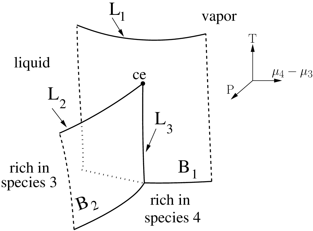
Taking the OPs to be independent of $l$ and omitting the surface fields, i.e., $f_{+}(l)=f_{-}(l)=0$, Eqs. (7) - (9), and Eqs. (14) - (16), together with the expression for the equilibrium free energy given by Eq. (13), render the bulk phase diagram of the system as studied in Ref. [34]. It has been demonstrated in Ref. [34] (see also Ref. [36]) that various coupling constants lead to diverse topologies of the phase diagram for the bulk liquid–liquid demixing transitions. The topologies discussed in Ref. [34] range from the phase diagram of a classical binary mixture (Figs. 4(a) and 5) to a phase diagram which to a large extent resembles the actual one of ${{}^{3}\text{He}}$ -${{}^{4}\text{He}}$ mixtures (Fig. 4 (b)). By extending the corresponding discussion in Ref. [34] one can study how, within the present model, for a suitable value of $J_{s}$ the bulk phase diagram of a classical binary mixture with specific values of $(C_{0}/K_{0},J_{0}/K_{0})$ and for $J_{s}=0$ (dotted curve in Fig. 6) transforms into that of the ${{}^{3}\text{He}}$-${{}^{4}\text{He}}$ mixture. Figure 6 illustrates schematically this transformation. One has to find and to adopt a nonzero value of $J_{s}=J_{s}^{0}$ such that the critical end point ce of the phase diagram for $(C_{0}/K_{0},J_{0}/K_{0},J_{s}=0)$ is in thermodynamic coexistence with a superfluid phase. This locates the critical end point ce on the right shoulder of the transformed phase diagram. Thus for $J_{s}>J_{s}^{0}$, the initial phase diagram for $(C_{0}/K_{0},J_{0}/K_{0},J_{s}=0)$ (including its critical end point ce), lies in the two–phase region of the phase diagram for $(C_{0}/K_{0},J_{0}/K_{0},J_{s}>J_{s}^{0})$ [37]. Although the phase diagram in Fig. 4 (b) satisfies the above condition and captures the main features of the bulk phase diagram of ${{}^{3}\text{He}}$-${{}^{4}\text{He}}$ mixtures, its shape near the tricritical end point tce differs from the experimental one (see Fig. 2). In particular, in the phase diagram in Fig. 4 (b), upon lowering the temperature below $T_{\text{tce}}$ along the path $X_{3}=X_{3}^{\text{tce}}$, the model mixture does not enter the two–phase region, as it is the case for the actual ${{}^{3}\text{He}}$-${{}^{4}\text{He}}$ mixture. Note that the experimental phase diagram in Fig. 2 is drawn in the $(T,\mathcal{C}_{3})$ plane. (The model phase diagram in the same $(T,\mathcal{C}_{3})$ plane is shown in the inset of Fig. 4 (b)) Furthermore, although the condition $J_{s}>J_{s}^{0}$ places the critical end point ce of the phase diagram with $(C_{0}/K_{0},J_{0}/K_{0},J_{s}=0)$ into the two–phase region of the phase diagram with $(C_{0}/K_{0},J_{0}/K_{0},J_{s}>J_{s}^{0})$, a certain residual, distorting influence of this critical end point ce on the wetting films may still be present, especially if ce lies near any of the two binodals of the demixing transitions of the transformed phase diagram (solid black lines in Figs. 4(b) and (c)). In order to address this issue, after finding the necessary conditions for the coupling parameters leading to the desired topology, we have modified the values of $(C_{0}/K_{0},J_{0}/K_{0})$ with $J_{s}=J_{s}^{0}$ such, that the critical end point ce (which starts to shift into metastablity for $J_{s}=J_{s}^{0}$) moves deeply into the two-phase region of the transformed phase diagram. These considerations have led us to choosing the following choice for the coupling constants: $(C/K,J/K,J_{s}/K)=(1,9.10714,3.70107)$. The corresponding phase diagram is shown in Fig. 4 (c).

In this subsection we consider a classical binary liquid mixture of species $3$ and $4$, described by the Hamiltonian given in Eq. (3) with the coupling constants $(C/K,J/K,J_{s}/K)=(1,5.714,0)$. The bulk phase diagram of this system in the $(T,X_{3})$ plane is shown in Fig. 4(a). All figures in this subsection (i.e., Figs. 7 - 11) share the coupling constants $(C/K,J/K,J_{s}/K)=(1,5.714,0)$. In Figs. 7(a) and 8 - 11 the system size is $L=40$, whereas in Fig. 7(b) it is $L=80$. We study how the strengths of the surface fields influence the formation of the wetting films for thermodynamic states with $T>T_{\text{ce}}$ and $\Delta\mu_{+}=\mu_{+}-\mu_{+}^{\text{co}}<0$, i.e., corresponding to the vapor being the bulk phase and the wetting phase being the mixed supercritical liquid phase.

We start our discussion by taking $\tilde{f_{-}}=0$ and varying $\tilde{f_{+}}$. We find that weak surface fields $\tilde{f_{+}}$ cannot stabilize high density layers near the surface, so that the model does not exhibit wetting by the mixed–liquid phase. Instead, for weak $\tilde{f}_{+}$ the wall prefers the vapor phase so that upon approaching the liquid–vapor coexistence from the liquid side (i.e., $\Delta\mu_{+}\to 0^{+}$) a vapor film forms close to the wall corresponding to drying of the interface between the wall and the mixed liquid.

Covering the case of weak surface fields, Fig. 7(a) shows the number density profiles for $(\tilde{f_{+}},\tilde{f_{-}})/K=(0.857,0)$ at $\Delta\mu_{+}/K=(\mu_{+}-\mu_{+}^{\text{co}})/K=-8.57\times 10^{-4}$, i.e., on the vapor side for several temperatures above the $T_{\text{ce}}$ and at fixed $X_{3}=X_{3}^{\text{ce}}$. Figure. 7(b) shows the number density profiles for the same bulk system with the same surface fields but for $\Delta\mu_{+}/K=(\mu_{+}-\mu_{+}^{\text{co}})/K=+8.57\times 10^{-4}$ so that the stable bulk phase is liquid. Since the wall prefers the vapor phase, upon increasing $T$ a drying film forms at the surface of the solid substrate.

For larger values of $\tilde{f_{+}}$ (see Fig. 8), i.e., for $(\tilde{f_{+}},\tilde{f_{-}})/K=(5.143,0)$, at lower temperatures $T$ we find monotonically decaying density profiles without shoulder formation whereas at higher temperatures the density profiles tend to exhibit plateaus characteristic of wetting (see Fig. 8(a)). Note that in Figs. 8(a) and (b) the number density in the first layer as part of the wetting film decreases upon increasing $T$. This is in accordance with the fact that the density of the bulk liquid phase as the wetting phase decreases upon heating, whereas the bulk vapor density increases. The profiles $X_{l}=X_{4,l}-X_{3,l}$ shown in red and blue in Fig. 8(b) have local minima at $l=5$ and $l=9$, respectively. These minima occur approximately at the position of the emerging liquid-vapor interface (see the corresponding curves in panel (a)) and indicate that species of type $3$ preferentially accumulate at the liquid-vapor interface. Figures 8 (c) and (d) show the OP profiles for $(\tilde{f_{+}},\tilde{f_{-}})/K=(5.143,0.857)$ and $\Delta\mu_{+}/K=-8.57\times 10^{-4}$ at several values of the temperature. One can see that for positive values of $\tilde{f_{-}}$ both $D_{l}$ and $X_{l}$ are enhanced in the first layer. This corresponds to the preferential adsorption of species of type $4$ at the wall.

In order to see how the wetting films grow upon approaching the liquid-vapor coexistence surface, we fix $T$ and vary $\Delta\mu_{+}$. Figure 9 shows the film thickness $y/a$ versus $\Delta\mu_{+}$ for $(\tilde{f_{+}},\tilde{f_{-}})/K=(8.571,0)$ and for several temperatures; $y$ is calculated according to Eq. (18). For low temperatures, upon approaching the liquid-vapor coexistence surface the film thickness increases smoothly and reaches a plateau. This corresponds to incomplete wetting. The height of this plateau increases gradually upon increasing $T$ towards $7.097<T_{w}/K<7.123$, which corresponds to a critical wetting transition between incomplete and complete wetting [38]. The corresponding line of wetting transitions lies on the surface of the liquid–vapor transitions (B₁ in Fig. 5) between the critical end point ce and and the line of critical points of the liquid–vapor transitions (L₁ in Fig. 5). Note that Fig. 9 provides a semi–logarithmic plot so that the linear growth of the film thickness on this scale confirms the theoretically expected logarithmic growth of the film thickness $y\sim\log(|\Delta\mu_{+}|/K)$ for short–ranged surface fields [38]. At higher temperatures $T$ the film thickness does not increase smoothly anymore but rather exhibits jumps due to layering transition. Figure 10 shows the location of these layering transitions in the $(\mu_{+},T)$ plane for $(\tilde{f_{+}},\tilde{f_{-}})/K=(8.571,0)$. If a thermodynamic path passes through any of these lines the film thickness undergoes a small jump of the size $l\simeq 1$. Each line of the layering transitions ends at a critical point. Along thermodynamic paths, which pass by these critical points the jumps of the film thickness become rounded as for the green and red curves in Fig. 9. The color code in Fig. 10 does not carry a particular meaning; the lines are colored differently so that it is easier to distinguish them. The closer the system is to the liquid-vapor coexistence surface, i.e., the smaller $\Delta\mu_{+}$ is, the closer are the lines of layering transitions. Figure 11 shows how the increasing density of the layering transition lines affects the film thickness while varying the temperature at fixed values of $\Delta\mu_{+}/K=-8.57\times 10^{-8}$ and $X_{3}=X_{3}^{\text{ce}}=0.431$.

In order to describe wetting films of ${{}^{3}\text{He}}$ -${{}^{4}\text{He}}$ mixtures, we focus on systems exhibiting phase diagrams with nonzero values of $J_{s}$ as in Fig. 4(c) and we choose the surface fields $(\tilde{f_{+}},\tilde{f_{-}})/K=(10.714,16.071)$. All figures in this subsection (i.e., Figs. 12 - 18) share the coupling constants $(C/K,J/K,J_{s}/K)=(1,9.10714,3.70107)$, the surface fields $(\tilde{f_{+}},\tilde{f_{-}})/K=(10.714,16.071)$, and the system size $L=60$. The growth of wetting films upon approaching the liquid-vapor coexistence surface is illustrated in Fig. 12, where we have used Eq. (18) for defining the film thickness. For all temperatures considered, upon approaching liquid–vapor coexistence the wetting films become thicker: $y(\Delta_{+}\to 0^{-})\sim\kappa\text{ln}\frac{1}{|\Delta\mu_{+}|/K}$ with a significant temperature dependence of the amplitude $\kappa$. This is different from the situation in Fig. 9 with $J_{s}=0$, where only for sufficiently high temperatures (i.e., $T>T_{w}$) complete wetting occurs. This means that in Fig. 12 $T_{w}$ is below the considered temperature interval. Interestingly, in Fig. 12 at the reduced temperature $(T-T_{\text{tce}})/T_{\text{tce}}\approx-0.016$ the film thickness exhibits the most rapid increase upon approaching the liquid-vapor coexistence surface (see the red curve), whereas for higher and lower temperatures the growth of the film thickness is reduced, i.e., the amplitude $\kappa(T)$ introduced above has a maximum at $(T-T_{\text{tce}})/T_{\text{tce}}\approx-0.016$. This is different from what one observes in Fig. 9, where the thickness of the wetting film is, via $\kappa(T)$, a monotonically increasing function of $T$. Note that in Fig. 12 for the curves with $T\geq T_{\text{tce}}$ the number density of ${{}^{3}\text{He}}$ is fixed at $X_{3}=X_{3}^{\text{tce}}=0.20845$. However, for $T<T_{\text{tce}}$ the system phase separates and the number density of ${{}^{3}\text{He}}$ changes. Accordingly, in Fig. 12 for $(T-T_{\text{tce}})/T_{\text{tce}}=-0.016$ and $(T-T_{\text{tce}})/T_{\text{tce}}=-0.042$, the number density of ${{}^{3}\text{He}}$ on the superfluid branch of the binodal (Fig. 4(c)) is $X_{3}=0.201$ and $X_{3}=0.188$, respectively. The OP profiles for three temperatures at $\Delta\mu_{+}/K=-1.07\times 10^{-4}$ are shown in Fig. 13. Due to the large value of $\tilde{f_{-}}$, the number density $X_{4,l}$ of ${{}^{4}\text{He}}$ is enhanced near the wall and hence $X_{l}=X_{4,l}-X_{3,l}$ is large there. If the bulk liquid is in the normal fluid phase but close to either the $\lambda$-line for $T>T_{\text{tce}}$, or to the normal branch of the binodal (Fig. 4(c)) for $T<T_{\text{tce}}$, this enhancement induces symmetry breaking of the superfluid OP near the wall. At the liquid-vapor coexistence surface, this so-called surface transition occurs at temperatures $T_{\text{s}}(X_{3})$, which depend on the bulk number density $X_{3}$ of ${{}^{3}\text{He}}$ atoms or, equivalently, on the bulk concentration $\mathcal{C}_{3}$ of ${{}^{3}\text{He}}$ as $T_{\text{s}}(\mathcal{C}_{3})$ (see Fig. 14). With the bulk being in the vapor phase, the continuous surface transition occurs within the wetting film for offsets $\Delta\mu_{+}$ from the liquid-vapor coexistence surface smaller than a certain temperature dependent value, which is marked in Fig. 12 by the tick along the abscissa colored accordingly. Upon crossing the continuous surface transition one observes a nonzero profile $M_{l}$ in the wetting film (see Figs. 13(a) and (b)). For $T<T_{\text{tce}}$, for which the bulk liquid phase separates into a superfluid and a normal fluid phase, the OP profiles within the wetting films exhibit two plateaus, one corresponding to the superfluid phase (note the left plateau of $M_{l}$ in Fig. 13(c)) and the other one (on the right side) corresponding to the normal fluid phase. The minimum of the profile $X_{l}$ occurs at the emerging liquid-vapor interface at around (a) $l=31$, (b) $l=9$, and (c) $l=17$. This demonstrates the effective attraction of ${{}^{3}\text{He}}$ towards the emerging liquid-vapor interface, which suppresses the superfluid OP at the liquid–vapor interface. On the other hand the preference of the wall for ${{}^{4}\text{He}}$ enhances the superfluid OP there as if there would be a surface field acting on the superfluid OP, which is , however, not the case.

The experimental data [3], reproduced in Fig. 15, have been obtained at liquid-vapor coexistence along the paths of fixed concentration $\mathcal{C}_{3}$ of ${{}^{3}\text{He}}$ as shown in the inset of Fig. 14 by the vertical dotted lines. (Note that in Fig. 15 $X$ corresponds to the concentration of ${{}^{3}\text{He}}$, which here is denoted by $\mathcal{C}_{3}=(D-X)/(2D)=X_{3}/(X_{3}+X_{4})$. We have ignored the subscript $l$ because we are referring to the bulk values.) The thermodynamic paths of fixed ${{}^{3}\text{He}}$ concentration followed in our calculations are parallel to the experimental ones but are located in the vapor phase close to the liquid-vapor coexistence surface (like the brown surface in Fig. 1).

The film thickness versus temperature along a path with an offset $\Delta\mu_{+}/K=-1.07\times 10^{-4}$ parallel to the vertical black dashed line in Fig. 14 is shown in Fig. 16. Within the considered temperature range the system is above the wetting temperature $T_{\text{w}}$ (not shown in the figure). We find that at fixed $\mathcal{C}_{3}$ the variation of the film thickness with temperature is nonmonotonic. Upon increasing the temperature, for $T>T_{\text{s}}$, the film thickness increases. A much steeper increase of the film thickness, associated with a break in slope, occurs between $T_{\text{s}}$ and $T_{\text{tce}}$, where the TCFs emerge. (Note that due to the offset from liquid–vapor coexistence the sharp drop of $y/a$ occurs slightly below $T_{\text{tce}}$ (see Fig. 14).)

As discussed before, due to the surface transition close to $T_{\text{tce}}$ the superfluid OP becomes nonzero near the wall. This profile vanishes at the emerging liquid-vapor interface, where the ${{}^{3}\text{He}}$ atoms accumulate. This behavior corresponds to the non-symmetric, effective $(+,O)$ BCs for the superfluid order parameter $M_{l}$ in the wetting film. Therefore, the resulting TCF acting on the liquid-vapor interface is repulsive and leads to an increase of the film thickness. The maximum film thickness occurs at $T_{\text{peak}}/K\approx 8.3346$, which lies below $T_{\text{tce}}$ - in agreement with the experimental results (see Fig. 15) ($T_{\text{peak}}$ is defined as the mid point of the temperature range enclosing the maximum film thickness). $T_{\text{s}}$ denotes the temperature of the surface transition. Figure 17 shows how the offset value $\Delta\mu_{+}$ affects the equilibrium film thickness $y$. As expected, upon increasing the offset value, the film thickness decreases. Moreover $T_{\text{peak}}$ shifts towards lower temperatures.

Following the other thermodynamic paths indicated in Fig. 14 renders a distinct scenario. Figure 18 shows the film thickness $y$ versus temperature $T$ for two values of $\mathcal{C}_{3}>\mathcal{C}_{3}^{\text{tce}}$ (green curve and violet curve) at $\Delta\mu_{+}/K=-1.07\times 10^{-4}$. (As a reference, we plot also the results for $\mathcal{C}_{3}=\mathcal{C}_{3}^{\text{tce}}$ (black curve)). The maximum of each of these two curves occurs at a temperature close to the corresponding bulk demixing temperature denoted as $T_{\text{d}}^{(\text{n})}(\mathcal{C}_{3})$. (This slight deviation from $T_{\text{d}}(\mathcal{C}_{3})$ is due to the offset $\Delta\mu_{+}$ from the liquid-vapor coexistence surface.) The green curve corresponding to $\Delta\mathcal{C}_{3}=\mathcal{C}_{3}-\mathcal{C}_{3}^{\text{tce}}=0.0087$ joins the black one at $T/K\simeq T_{\text{d}}^{(\text{n})}(\mathcal{C}_{3})/K=8.3925$; for lower temperatures both curves merge. Since for the green curve $T_{\text{d}}^{(\text{n})}(\mathcal{C}_{3})>T_{\text{peak}}=8.3346$, the maximum of this curve is the same as the maximum of the black curve. However, for $\Delta\mathcal{C}_{3}=0.0257$ the violet curve joins the black curve at the corresponding demixing temperature $T_{\text{d}}^{(\text{n})}(\mathcal{C}_{3})/K=8.2392$, which is below the temperature $T_{\text{peak}}$ of the peak. Therefore, the maximum of the violet curve differs from the maximum of the black curve. Figure 18 corresponds to panel (a) in Fig. 15. Note that $X_{\text{t}}$ in Fig. 15 corresponds to $\mathcal{C}_{3}^{\text{tce}}$ in the present notation.

Figure 19 shows the film thickness as function of temperature for two values of $\mathcal{C}_{3}<\mathcal{C}_{3}^{\text{tce}}$ (red curve and blue curve; compare the inset in Fig. 14 with the same color code) and for $\mathcal{C}_{3}^{\text{tce}}$ (black curve) at $\Delta\mu_{+}/K=-1.07\times 10^{-4}$. The blue curve and the red curve merge with the black one at $T_{\text{d}}$ close to the demixing temperature denoted as $T_{\text{d}}^{(\text{s})}(\mathcal{C}_{3})$ in Fig. 14 (there is a slight deviation due to the offset from the liquid–vapor coexistence). Whereas for $\mathcal{C}_{3}\geq\mathcal{C}_{3}^{\text{tce}}$ the sudden drop of the film thickness occurs near $T_{\text{d}}^{(\text{n})}(\mathcal{C}_{3})$ (note that for $T_{\text{d}}^{(\text{s},\text{n})}(\mathcal{C}_{3}^{\text{tce}})=T_{\text{tce}}$), for $\mathcal{C}_{3}<\mathcal{C}_{3}^{\text{tce}}$ it takes place close to the bulk $\lambda$-transition temperature $T_{\lambda}(\mathcal{C}_{3})\geqslant T_{\text{tce}}$. (Again, there is a slight deviation due to the offset from the liquid-vapor coexistence surface.) This sudden drop is associated with a break in slope in the curves $y(T)$ and leads to the formation of characteristic shoulders. This agrees with the experimental observations (see panel (b) in Fig. 15). Note that because $T_{\lambda}(\mathcal{C}_{3})$ is a decreasing function of $\mathcal{C}_{3}$, for lower concentrations of ${{}^{3}\text{He}}$, the break in slope occurs at higher temperatures. For the red curve in Fig. 19, this shoulder is due to the emerging of the CCFs close to the $\lambda$-line. For even lower values of $\mathcal{C}_{3}$ the films encounter only the CCFs due to the $\lambda$–transition and the TCFs due to the tricritical point do not influence them (see the blue curve). In Fig. 19 all curves attain their lowest value at the surface transition temperature $T_{\text{s}}(\mathcal{C}_{3})>T_{\lambda}(\mathcal{C}_{3})$.

For a vertical path at $\mathcal{C}_{3}<\mathcal{C}_{3}^{\text{s*}}$ (see Fig. 14), the film thickness does not exhibit an increase near the ${\lambda}$–transition. In fact, for $\mathcal{C}_{3}<\mathcal{C}_{3}^{\text{s*}}$ the BCs for the superfluid OP at the interface of the wetting film are the symmetric (O,O) BCs (i.e., $M=0$ at the wall and at the emerging liquid-vapor interface). Therefore, in this regime one expects the occurrence of an attractive CCF; however, this cannot be captured within the present mean field approximation because for Dirichlet–Dirichlet BCs the resulting CCF is solely due to fluctuations beyond mean field theory [15, 16]. Although both black curves in Fig. 18 and 19 correspond to $\mathcal{C}_{3}=\mathcal{C}_{3}^{\text{tce}}$, they differ slightly due to the infinitesimal difference of the thermodynamic paths for $T<T_{\text{tce}}$. In Fig. 18, for $T<T_{\text{tce}}$ the thermodynamic paths follow the demixing line $T_{\text{d}}^{(\text{n})}(\mathcal{C}_{3})$ infinitesimally on the normal fluid side, whereas in Fig. 19 for $T<T_{\text{tce}}$ the thermodynamic paths run along the superfluid binodal $T_{\text{d}}^{(\text{s})}(\mathcal{C}_{3})$.

A fluid film exerts an effective force on its confining walls. For two parallel, planar walls a distance $L$ apart this fluid mediated force $f_{s}$ is given by [40]

where $f_{\text{b}}$ is the grand canonical bulk free energy density of a one–component fluid at temperature $T$ and chemical potential $\mu$. ${\cal F}$ is the free energy of the film of volume $V={\cal A}L$ where ${\cal A}$ is the macroscopically large surface area of one wall. Since $\mathcal{F}-Vf_{b}$ is proportional to $\mathcal{A}$, $f_{\text{s}}/{\cal A}$ is the pressure in excess over its bulk value. Upon approaching the bulk critical point of the confined fluid, $f_{\text{s}}$ acquires a universal long-ranged contribution $f_{C}$, known as the critical Casimir force [41, 18, 42].

Extending this concept to binary liquid mixtures, here we focus on that contribution to $f_{\text{s}}/{\cal A}$ which arises near a tricritical point of ${{}^{3}\text{He}}$ - ${{}^{4}\text{He}}$ mixtures. We call this contribution tricritical Casimir force $f_{\text{tcr}}$ (TCF) and express it in units of $k_{\text{B}}T_{\text{tc}}$, where $T_{\text{tc}}$ is the temperature of a tricritical point on the line TC in Fig. 1.

As discussed in the Introduction, concerning wetting by a critical fluid, the critical fluctuations of the OP are confined by the solid substrate surface on one side and by the emerging liquid-vapor interface on the other side. Accordingly, the TCF is the derivative of the corresponding excess free energy with respect to the film thickness $y$ at constant temperature and chemical potentials. In contrast to the slab geometry with two fixed walls as discussed above (see Eq. (20)), varying the equilibrium wetting film thickness requires to change the thermodynamic state of the fluid. Moreover, in the present microscopic approach the film thickness is not an input parameter of a model; hence, the excess free energy is not an explicit function of $y$. (Note that $y$ is uniquely defined in terms of the equilibrium density profile $D_{l}(T,\mu_{+},\mu_{-})$ via Eq. (18).) In order to calculate the TCF, we consider a system at fixed $T,\mu_{+}$, and $\mu_{-}$, for which the film thickness is fixed to a specific value $\ell$ by an externally imposed constraint. For the total free energy $F_{\text{cstr}}$ of such a constraint system, one has for large $L$ [1, 16, 43]

where $\sigma_{\text{w,l}}$ and $\sigma_{\text{l,v}}$ are the wall-liquid and vapor-liquid surface tensions, respectively, $f_{\text{m}}$ is the free energy density of the metastable liquid, and $A:=\mathcal{N}a^{2}$ is the cross section area of a layer. Since at liquid–vapor coexistence $f_{\text{b}}=f_{\text{vapor}}=f_{\text{liquid}}<f_{\text{m}}$ one has $(f_{\text{m}}-f_{\text{b}})l>0$. The $\ell$-dependent excess free energy $f_{\text{ex}}(\ell)$ is the sum of two contributions: the free energy density (per area $A$) $f_{0}(\ell)$ due to the effective interaction of the emerging liquid–vapor interface with the substrate wall and the singular contribution $f_{\text{sing}}(\ell)$ due to the critical finite-size effects within the wetting film of thickness $l$. For short–ranged surface fields, the effective potential between the wall and the emerging liquid-vapor interface is an exponentially decaying function of the film thickness $\ell$. To leading order one has [44]

References

- [1] M. Krech and S. Dietrich, Phys. Rev. A 46, 1922 (1992).
- [2] R. Garcia and M. H. W. Chan, Phys. Rev. Lett. 83, 1187 (1999).
- [3] R. Garcia and M. H. W. Chan, Phys. Rev. Lett. 88, 086101 (2002).
- [4] A. Ganshin, S. Scheidemantel, R. Garcia, and M. H. W. Chan, Phys. Rev. Lett. 97, 075301 (2006).
- [5] M. Fukuto, Y. F. Yano, and P. S. Pershan, Phys. Rev. Lett. 94, 135702 (2005).
- [6] S. Rafaï, D. Bonn, and M. J., Physica 386, 31 (2007).
- [7] A. Mukhopadhyay and B. M. Law, Phys. Rev. Lett. 83, 772 (1999).
- [8] A. Mukhopadhyay and B. M. Law, Phys. Rev. E 62, 5201 (2000).
- [9] M. E. Fisher and P. G. de Gennes, C. R. Seances Acad. Sci. Paris Ser. B 287, 207 (1978).
- [10] K. Binder, in Phase Transitions and Critical Phenomena, edited by C. Domb and J. L. Lebowitz (Academic, London, 1983), Vol. 8, p. 149.
- [11] V. Privman, in Finite Size Scaling and Numerical Simulation of Statistical Systems, edited by V. Privman (World Scientific, Singapore, 1990), p. 1.
- [12] H. Casimir, Proc. K. Ned. Akad. Wet 51, 793 (1948).
- [13] M. Krech, The Casimir effect in critical systems (World Scientific, Singapore, 1994).
- [14] M. P. Nightingale and J. O. Indekeu, Phys. Rev. Lett. 54, 1824 (1985).
- [15] M. Krech and S. Dietrich, Phys. Rev. Lett. 66, 345 (1991).
- [16] M. Krech and S. Dietrich, Phys. Rev. A 46, 1886 (1992).
- [17] H. W. Diehl, in Phase Transitions and Critical Phenomena, edited by C. Domb and J. L. Lebowitz (Academic, London, 1986), Vol. 10, p. 75.
- [18] J. G. Brankov, D. Danchev, and N. Tonchev, Theory of critical phenomena in finite–size systems (World Scientific, Singapore, 2000).
- [19] R. Zandi, J. Rudnick, and M. Kardar, Phys. Rev. Lett. 93, 155302 (2004).
- [20] A. Maciołek, A. Gambassi, and S. Dietrich, Phys. Rev. E 76, 031124 (2007).
- [21] R. Zandi, A. Shackell, J. Rudnick, M. Kardar, and L. P. Chayes, Phys. Rev. E 76, 030601(R) (2007).
- [22] O. Vasilyev, A. Gambassi, A. Maciołek, and S. Dietrich, EPL 80, 60009 (2007).
- [23] O. Vasilyev, A. Gambassi, A. Maciołek, and S. Dietrich, Phys. Rev. E 79, 041142 (2009).
- [24] D. Dantchev and M. Krech, Phys. Rev. E 69, 046119 (2004).
- [25] A. Hucht, Phys. Rev. Lett. 99, 185301 (2007).
- [26] M. Hasenbusch, J. Stat. Mech.: Theory and Experiment 2009, P07031 (2009).
- [27] M. Hasenbusch, Phys. Rev. B 81, 165412 (2010).
- [28] J. P. Romagnan, J. P. Laheurte, J. C. Noiray, and W. F. Saam, J. Low Temp. Phys. 30, 425 (1978).
- [29] A. Maciołek and S. Dietrich, Europhys. Lett. 74, 22 (2006).
- [30] A. Maciołek, A. Gambassi, and S. Dietrich, Phys. Rev. E 76, 031124 (2007).
- [31] M. Blume, V. J. Emery, and R. B. Griffiths, Phys. Rev. A 4, 1071 (1971).
- [32] A. N. Berker and D. R. Nelson, Phys. Rev. B 19, 2488 (1979).
- [33] J. L. Cardy and D. J. Scalapino, Phys. Rev. B 19, 1428 (1979).
- [34] N. Farahmand Bafi, A. Maciołek, and S. Dietrich, Phys. Rev. E 91, 022138 (2015).
- [35] M. Galassi, J. Davies, J. Theiler, B. Gough, G. Jungman, P. Alken, M. Booth, and F. Rossi, GNU Scientific Library Reference Manual, Network Theory Ltd., 2009; library available online at http://www.gnu.org/software/gsl/.
- [36] A. Maciołek, M. Krech, and S. Dietrich, Phys. Rev. E 69, 036117 (2004).
- [37] G. M. Bell and D. A. Lavis, Statistical mechanics of lattice models,Vol.1, (Springer, Chichester, 1989).
- [38] S. Dietrich, in Phase Transitions and Critical Phenomena, edited by C. Domb and J. L. Lebowitz (Academic, London, 1988), Vol. 12, p. 1.
- [39] S. Dietrich, in Phase Transitions in Surface Films 2, proceedings of the NATO ASI (Series B) held in Erice, Italy, 19-30 June 1990, edited by H. Taub, G. Torzo, H. J. Lauter, and S. C. Fain (Plenum, New York, 1991), Vol. B 267, p. 391.
- [40] R. Evans, J. Phys.: Condens. Matter 2, 8989 (1990).
- [41] M. Krech, Phys. Rev. E 56, 1642 (1997).
- [42] A. Gambassi, J. Phys.: Conf. Series 161, 012037 (2009).
- [43] S. Dietrich and M. Napiórkowski, Phys. Rev. A 43, 1861 (1991).
- [44] K. Binder, D. Landau, and M. Müller, J. Stat. Phys. 110, 1411 (2003).
- [45] E. K. Riedel, Phys. Rev. Lett. 28, 675 (1972).
- [46] I. D. Lawrie and S. Sarbach, in Phase Transitions and Critical Phenomena, edited by C. Domb and J. L. Lebowitz (Academic, London, 1984), Vol. 9, p. 2.
- [47] P. M. Chaikin and T. Lubensky, Principles of condensed matter physics (Cambridge University press, Cambridge, 1995).
- [48] M. Abramowitz and I. A. Stegun, eds., Handbook of mathematical functions (Dover, New York, 1972).