Dyck Paths and Positroids
from Unit Interval Orders
Abstract.
It is well known that the number of non-isomorphic unit interval orders on equals the -th Catalan number. Using work of Skandera and Reed and work of Postnikov, we show that each unit interval order on naturally induces a rank positroid on . We call the positroids produced in this fashion unit interval positroids. We characterize the unit interval positroids by describing their associated decorated permutations, showing that each one must be a -cycle encoding a Dyck path of length . We also provide recipes to read the decorated permutation of a unit interval positroid from both the antiadjacency matrix and the interval representation of the unit interval order inducing . Using our characterization of the decorated permutation, we describe the Le-diagrams corresponding to unit interval positroids. In addition, we give a necessary and sufficient condition for two Grassmann cells parameterized by unit interval positroids to be adjacent inside the Grassmann cell complex. Finally, we propose a potential approach to find the -vector of a unit interval order.
Key words and phrases:
Positroid, Dyck path, unit interval order, decorated permutation, Le diagram, positive Grassmannian1. Introduction
A unit interval order is a partially ordered set that captures the order relations among a collection of unit intervals on the real line. Unit interval orders originated in the study of psychological preferences, first appearing in the work of Wiener [18], and then in greater detail in the work of Armstrong [4] and others. They were also studied by Luce [10] to axiomatize a class of utilities in the theory of preferences. Since then they have been systematically studied (see [5, 6, 7, 8, 19, 16] and references therein). These posets exhibit many interesting properties; for example, they can be characterized as the posets that are simultaneously -free and -free (see Section 2). Moreover, it was first proved in [19] that the number of non-isomorphic unit interval orders on equals , the -th Catalan number (see also [5, Section 4]).
In [16], motivated by the desire to understand the -vectors of various classes of posets, Skandera and Reed showed that a simple procedure for labeling a unit interval order yields the useful form of its antiadjacency matrix which is totally nonnegative (i.e., has all its minors nonnegative) with its zero entries appearing in a right-justified Young diagram located strictly above the main diagonal and anchored in the upper-right corner. The zero entries of such a matrix are separated from the one entries by a Dyck path joining the upper-left corner to the lower-right corner. Motivated by this observation, we call such matrices Dyck matrices. The Hasse diagram and the antiadjacency (Dyck) matrix of a canonically labeled unit interval order are shown in Figure 1.


On the other hand, it follows from work of Postnikov [12] that the antiadjacency (Dyck) matrix of a (properly labeled) unit interval order can be regarded as representing a rank positroid on the ground set . We will say that such a positroid is induced by . Positroids, which are special matroids, were introduced and classified by Postnikov in his study of the totally nonnegative part of the Grassmannian [12]. He showed that there is a cell decomposition of the totally nonnegative part of the Grassmannian so that cells are indexed by positroids (or equivalent combinatorial objects). Positroids and the nonnegative Grassmannian have been the subject of a great deal of recent work, with connections and applications to cluster algebras [15], scattering amplitudes [3], soliton solutions to the Kadomtsev-Petviashvili equation [9], and free probability [2].
In this paper we characterize the positroids that arise from unit interval orders, which we call unit interval positroids. We show that the decorated permutations associated to rank unit interval positroids are certain -cycles in bijection with Dyck paths of length . The following theorem is a formal statement of our main result (the necessary definitions are given in Section 2).
Main Theorem.
A decorated permutation represents a unit interval positroid on if and only if is a -cycle satisfying the following two conditions:
- (1)
in the sequence the elements appear in increasing order while the elements appear in decreasing order;
- (2)
for every , the set contains at least as many elements of the set as elements of the set .
In particular, there are unit interval positroids on .
The decorated permutation associated to a unit interval positroid on induced by a unit interval order naturally encodes a Dyck path of length . Here we provide a recipe to read this decorated permutation directly from the Dyck path appearing in the antiadjacency (Dyck) matrix of . We will refer to this path as the semiorder path of .
Theorem 1.1.
Let be a canonically labeled unit interval order on , and let be its antiadjacency matrix. Number the vertical steps of the semiorder path of from bottom to top by and label the horizontal steps from left to right by . Then the sequence of labels, read in the northwest direction, is the decorated permutation associated to the unit interval positroid induced by .
Example 1.2.
The vertical assignment on the left of Figure 2 shows a set of unit intervals along with a canonically labeled unit interval order on describing the order relations among the intervals in (see Theorem 2.2). The vertical assignment on the right illustrates the recipe given in Theorem 1.1 to read the decorated permutation associated to the unit interval positroid induced by directly from the antiadjacency matrix. Note that the decorated permutation is a -cycle satisfying conditions (1) and (2) of our main theorem. The solid and dashed assignment signs represent functions that we shall introduce later.

This paper is organized as follows. In Section 2 we establish the notation and formally present the fundamental concepts and objects used throughout this paper. Then, in Section 3, we formally introduce canonical labelings and canonical interval representations of unit interval orders. Also, we use canonical labelings to exhibit an explicit bijection from the set of non-isomorphic unit interval orders on to the set of Dyck matrices. Section 4 is dedicated to the description of the unit interval positroids via their decorated permutations, which yields the direct implication of the main theorem. In Section 5, we show how to read the decorated permutation associated to a unit interval positroid from either an antiadjacency matrix or a canonical interval representation of the corresponding unit interval order, which allows us to complete the proof of the main theorem. Then, in Section 6, we characterize the Le-diagrams of unit interval positroids. In Section 7, we find a necessary and sufficient condition for two unit interval positroids to index adjacent cells in the cell decomposition of the totally nonnegative part of the Grassmannian. Finally, in Section 8, we interpret the -vector of a poset in terms of its antiadjacency matrix and, based on this, we propose a potential approach to compute the -vector of a unit interval order.
2. Background and Notation
For ease of notation, when is a partially ordered set (poset for short), we just write , tacitly assuming that the order relation on is to be denoted by the symbol . For , we will write when and . In addition, every poset showing up in this paper is assumed to be finite.
Definition 2.1.
A poset is a unit interval order if there exists a bijective map from to a set of closed unit intervals of the real line such that for , if and only if . We then say that is an interval representation of .
For each , we denote by the set of all non-isomorphic unit interval orders of cardinality . For nonnegative integers and , let denote the poset which is the disjoint sum of an -element chain and an -element chain. Let and be two posets. We say that is an induced subposet of if there exists an injective map such that for all one has if and only if . By contrast, is a -free poset if does not contain any induced subposet isomorphic to . The following theorem provides a useful characterization of the elements of .
Theorem 2.2.
[13, Theorem 2.1] A poset is a unit interval order if and only if it is simultaneously -free and -free.
If the poset has cardinality , then a bijective function is called an -labeling of ; after identifying with via , we say that is an -labeled poset. The -labeled poset is naturally labeled if implies that as integers for all .
Example 2.3.
The figure below depicts the -labeled unit interval order introduced in Figure 1 with a corresponding interval representation.


Another useful way of representing an -labeled unit interval order is through its antiadjacency matrix.
Definition 2.4.
If is an -labeled poset, then the antiadjacency matrix of is the binary matrix with if and only if .
Recall that a binary square matrix is said to be a Dyck matrix if its zero entries are separated from its one entries by a Dyck path joining the upper-left corner to the lower-right corner. We call such a Dyck path the semiorder path of . All minors of a Dyck matrix are nonnegative (see, for instance, [1]). We denote by the set of all Dyck matrices. As presented in [16], every unit interval order can be naturally labeled so that its antiadjacency matrix is a Dyck matrix (details provided in Section 3). This yields a natural map that is a bijection (see Theorem 3.5). In particular, is the -th Catalan number, which can also be deduced from the one-to-one correspondence between Dyck matrices and their semiorder (Dyck) paths.
For any matrix and any -element subsets , of row and column indices of , define , the ,-minor of to be the determinant of the submatrix of determined by rows and columns . Let denote the set of all full rank real matrices with nonnegative maximal minors. Given a totally nonnegative real matrix , there is a natural assignment , where .
Lemma 2.5.
Using Lemma 2.5 and the aforementioned map , we can assign via a matrix of to each unit interval order of cardinality . In turn, every real matrix of gives rise to a positroid, a special representable matroid which has a very rich combinatorial structure. Let us recall the concept of matroid.
Definition 2.6.
Let be a finite set, and let be a nonempty collection of subsets of . The pair is a matroid if for all and , there exists such that .
If is a matroid, then is called the ground set of and the elements of are called bases of . Any two bases of have the same size, which we denote by and call the rank of . If and , then we say that is representable if there exists a real matrix with columns such that precisely when is a basis for the vector space .
Definition 2.7.
The rank matroid on the ground set represented by a matrix is denoted by and called a positroid.
Each unit interval order (labeled so that its antiadjacency matrix is a Dyck matrix) induces a positroid via Lemma 2.5, namely, the positroid represented by the matrix .
Definition 2.8.
A positroid on induced by a unit interval order is called a unit interval positroid.
We denote by the set of all unit interval positroids on the ground set . The function plays a fundamental role in this paper. Indeed, we will end up proving that this function is a bijection (see Theorem 5.4).
Several families of combinatorial objects, in bijection with positroids, were introduced in [12] to study the totally nonnegative Grassmannian: decorated permutations, Grassmann necklaces, Le-diagrams, and plabic graphs. We use decorated permutations, obtained from Grassmann necklaces, to provide a compact and elegant description of unit interval positroids.
In the next definition subscripts should be interpreted modulo .
Definition 2.9.
Let such that . An -tuple of -subsets of is called a Grassmann necklace of type if for every the following conditions hold:
- •
implies for some ;
- •
implies .
For , the total order on defined by is called the shifted linear -order. For a matroid of rank , one can define the sequence , where is the lexicographically minimal ordered basis of with respect to the shifted linear -order. It was proved in [12, Section 16] that the sequence is a Grassmann necklace of type . We call the Grassmann necklace associated to . When is a positroid we can recover from its Grassmann necklace via Theorem 2.10; however, this does not hold for a general matroid, which can be deduced also from Theorem 2.10.
For , the Gale order on with respect to is the partial order defined in the following way. If and , then if and only if for each .
Theorem 2.10.
[11, Theorem 6] For such that , let be a Grassmann necklace of type . Then
is the collection of bases of a positroid , where is the Gale -order on . Moreover, for all positroids .
Therefore there is a natural bijection between positroids on of rank and Grassmann necklaces of type . However, decorated permutations, also in one-to-one correspondence with positroids, will provide a more succinct representation.
Definition 2.11.
A decorated permutation of is an element whose fixed points are marked either “clockwise” (denoted by ) or “counterclockwise” (denoted by ).
A weak -excedance of a decorated permutation is an index satisfying or . It is easy to see that the number of weak -excedances does not depend on , so we just call it the number of weak excedances.
To every Grassmann necklace one can associate a decorated permutation as follows:
- •
if , then ;
- •
if and , then ;
- •
if and , then .
The assignment defines a one-to-one correspondence between the set of Grassmann necklaces of type and the set of decorated permutations of having exactly weak excedances.
Proposition 2.12.
[2, Proposition 4.6] The map is a bijection between the set of Grassmann necklaces of type and the set of decorated permutations of having exactly weak excedances.
Definition 2.13.
If is a positroid and is the Grassmann necklace associated to , then we call the decorated permutation associated to .
3. Canonical Labelings on Unit Interval Orders
In this section we introduce the concept of a canonically labeled poset, and we use it to exhibit an explicit bijection from the set of non-isomorphic unit interval orders of cardinality to the set of Dyck matrices.
Given a poset and , the order ideal and the dual order ideal of are defined to be and , respectively. We define the altitude function of to be the map defined by . We say that an -labeled poset respects altitude if for all , the fact that implies (as integers). Notice that every poset can be labeled by the set such that, as an -labeled poset, it respects altitude (see also [6, p. 33]).
Definition 3.1.
An -labeled poset is canonically labeled if it respects altitude.
Each canonically -labeled poset is, in particular, naturally labeled. The next proposition, extending [17, proof of Theorem 2.11], characterizes canonically -labeled unit interval orders in terms of their antiadjacency matrices.
Proposition 3.2.
[16, Proposition 5] An -labeled unit interval order is canonically labeled if and only if its antiadjacency matrix is a Dyck matrix.
The above proposition indicates that the antiadjacency matrices of canonically labeled unit interval orders are quite special. In addition, canonically labeled unit interval orders have very convenient interval representations.
Proposition 3.3.
Let be an -labeled unit interval order. Then the labeling of is canonical if and only if there exists an interval representation of such that .
Proof.
Let be the altitude map of . For the forward implication, suppose that the -labeling of is canonical. Among all interval representations of , assume that gives the maximum such that . Suppose, by way of contradiction, that . The maximality of implies that . This, along with the fact that , ensures that . Similarly, for any ; otherwise
would contradict that the -labeling of respects altitude. An analogous argument guarantees that for any .
Now take to be the smallest natural number in such that for all , and take . We will show that , where , is an interval representation of . Take such that . Since and are comparable in , at least one of them must be fixed by ; say . If , then . Also, if , then . It follows from that . The case of can be argued similarly. Thus, is an interval representation of . As , the definition of implies that , which contradicts the maximality of . Hence , and the direct implication follows.
Conversely, note that if is an interval representation of satisfying , then for every we have
which means that the labeling of is canonical. ∎
If is a canonically -labeled unit interval order, and is an interval representation of satisfying , then we say that is a canonical interval representation of .
Note that the image (as a multiset) of the altitude map does not depend on the labels but only on the isomorphism class of a poset. On the other hand, the altitude map of a canonically -labeled unit interval order satisfies . Thus, if is a canonically -labeled unit interval order isomorphic to , then
| (3.1) |
where is the altitude map of . Let and be the antiadjacency matrices of and , respectively. As , the first rows of and are equal. Since the number of zeros in the -th column (resp., -th row) of is precisely (resp., ), and similar statement holds for , the next lemma follows immediately by using (3.1) and induction on the row index of and .
Lemma 3.4.
If two canonically labeled unit interval orders are isomorphic, then they have the same antiadjacency matrix.
Now we can define a map , by assigning to each unit interval order its antiadjacency matrix with respect to any of its canonical labelings. By Lemma 3.4, this map is well defined.
Theorem 3.5.
For each natural number , the map is a bijection.
4. Description of Unit Interval Positroids
We proceed to describe the decorated permutation associated to a unit interval positroid. Throughout this section is an Dyck matrix and is as in Lemma 2.5. We will consider the indices of the columns of modulo . Furthermore, let be the unit interval positroid represented by , and let and be the Grassmann necklace and the decorated permutation associated to .
Lemma 4.1.
For , the -th coordinate set of does not contain .
Proof.
It is not hard to verify that every matrix resulting from removing one column from still has rank . As the matrix obtained by removing the -st column from has rank , it contains linearly independent columns. Therefore the lemma follows straightforwardly from the -minimality of the -th coordinate set of . ∎
For the rest of this section let denote the -th column of . As a direct consequence of Lemma 4.1, we have that does not have any counterclockwise fixed point. On the other hand, cannot have any clockwise fixed point because every column of is nonzero. Hence (and therefore ) does not fix any point. The next lemma immediately follows from the way is produced from the Grassmann necklace (see the end of Section 2).
Lemma 4.2.
For , equals the minimum with respect to the -order such that .
Now we find an explicit expression for the function representing the inverse of the decorated permutation associated to . In order to do so, we will find it convenient to associate an index set and a map to the matrix . We define the set of principal indices of to be the subset of defined by
We associate to the weight map defined by ; more explicitly, we obtain that
Since the last row of the antiadjacency matrix has all its entries equal to , the map is well defined. If , then is the number of nonzero entries in the column . Now we have the following formula for .
Proposition 4.3.
For , we have
The index in the final case is necessarily unique.
Proof.
First, suppose that and . Then we have and the set is linearly dependent. Lemma 4.2 then implies that .
Now suppose that and . Then results from replacing () of the last nonzero entries of by zeros. Since , the indices and both appear in the -th coordinate set of . Also, because the columns are linearly dependent, not all the indices appear in the -th coordinate set of . On the other hand, at most one index in is missing from the -th coordinate of ; this is because the submatrix of determined by the row-index set and the column-index set has rank . By the minimality of the -th coordinate set of with respect to the -order, the index of missing in the -th coordinate set of is . As a result, we have ; otherwise, in the submatrix of whose columns are indexed by the -st coordinate set of , the -th row would consist entirely of zeros, which, in turn, would contradict the fact that such a coordinate set represents a basis of the positroid .
The above argument also applies when provided that we extend the domain of to and set .
Note that follows immediately from the minimality of the second coordinate set of and the fact that are linearly independent.
Now suppose that and . The minimality of the coordinate sets of implies that all the indices appear in the -th coordinate set. Furthermore, Lemma 4.1 implies that does not belong to the -th coordinate set of . Since no has weight , the -st and -th rows of the maximal submatrix of determined by the column index set are equal. Consequently, we have ; otherwise the associated maximal submatrix of determined by the indices of the -th coordinate set of would have the -th and -st rows identical, which would contradict the fact that the -th coordinate set of represents a basis of .
Finally, suppose that and . Since not two elements of have the same weight, there is at most one such that . As before, all the indices appear in the -th coordinate set of (because ). Each column , for such that , is a linear combination of the columns . Therefore such indices do not appear in the -th coordinate set of . By Lemma 4.1, it follows that does not appear in the -th coordinate set of . Thus, , where satisfies that ; otherwise, in the submatrix of whose columns are indexed by the -st coordinate set of , the -st row would consist entirely of zeros, which would contradict that the -st coordinate set of represents a basis of . By minimality of the -st coordinate set of one finds that . ∎
As the next theorem indicates, is a -cycle satisfying a very special property.
Theorem 4.4.
is a -cycle satisfying the next two conditions:
- (1)
in the sequence the elements appear in increasing order while the elements appear in decreasing order;
- (2)
for every , the set contains at least as many elements of the set as elements of the set .
Proof.
From Proposition 4.3 we immediately deduce that if for , then when and when . This implies, in particular, that . Suppose, by way of contradiction, that , and so , is not a -cycle. Then there is a cycle in the canonical cycle-type decomposition of that does not contain . Therefore one has
which implies . Since does not contain , it follows that , which is a contradiction. Hence the cycle-type decomposition of contains only one cycle, which has length .
Since , one gets that , where is precisely the set . As
and for every , the elements of the set must appear in the cycle in decreasing order. On the other hand, by Proposition 4.3 the indices of equal columns of (but perhaps the first one) show in increasing order and consecutively in the sequence . Also, as the weight map is strictly decreasing when restricted to , the elements of the set must appear in increasing order in the cycle . Thus, condition (1) holds.
To show condition (2), write and suppose, by way of contradiction, that there exists such that
| (4.1) |
Let be the minimal such index. By the minimality of , one obtains that . Let be the maximum index such that and for each . Note that and . Since
and
it follows by (4.1) that , which implies . On the other hand, the fact that all the entries of below and on the main diagonal equal implies that for every . Since , one finds that . As , we have
which is a contradiction. Hence, writing , we will obtain that for , the set contains at least as many elements of the set as elements of the set , which is condition (2). ∎
5. A Direct Way to Read The Unit Interval Positroid
Throughout this section, let be a canonically -labeled unit interval order with antiadjacency matrix . Also, let be a canonical interval representation of (i.e., ); Proposition 3.3 ensures the existence of such an interval representation. In this section we describe a way to obtain the decorated permutation associated to the unit interval positroid induced by directly from either or . Such a description will reveal that the function introduced in Section 2 is a bijection (Theorem 5.4).
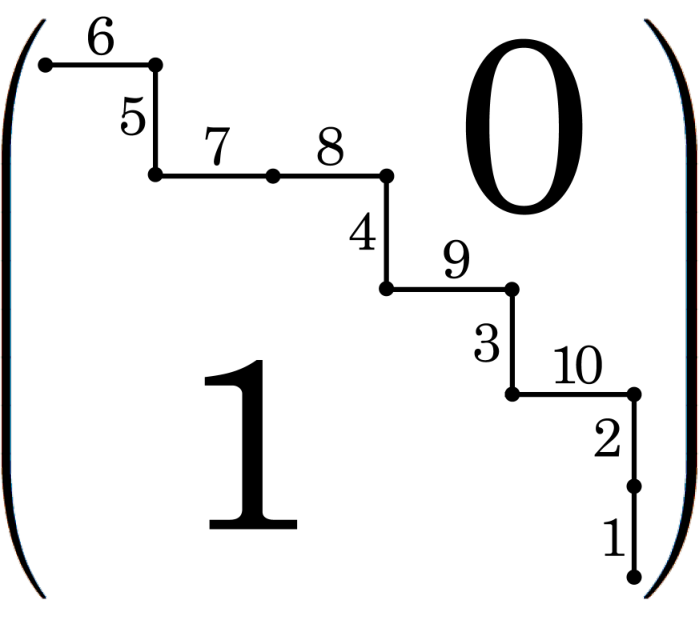
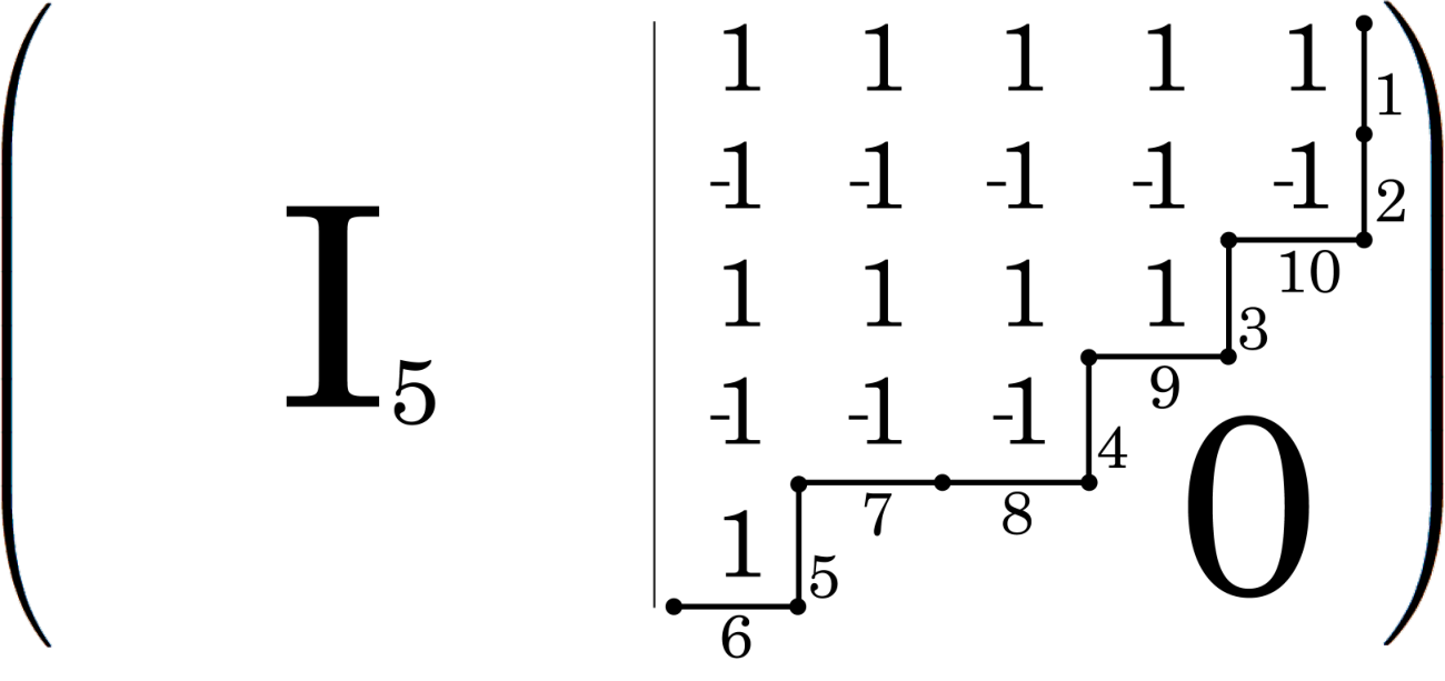
Recall that the north and east borders of the Young diagram formed by the nonzero entries of give a path of length that we call the semiorder path of . Let , where is the map introduced in Lemma 2.5. We will also associate a second path to . Let the inverted path of be the path consisting of the south and east borders of the Young diagram formed by the nonzero entries of . Note that the inverted path of is just the reflection in a horizontal line of the semiorder path of . Example 5.2 sheds light upon the statement of the next theorem, which describes a way to find the decorated permutation associated to the unit interval positroid induced by directly from .
Theorem 5.1.
If we number the vertical steps of the semiorder path of from bottom to top in increasing order with and the horizontal steps from left to right in increasing order with , then by reading the semiorder path in the northwest direction, we obtain the decorated permutation associated to the unit interval positroid induced by .
Proof.
Let be the decorated permutation associated to the unit interval positroid induced by . Label the vertical steps of the inverted path of from top to bottom in increasing order using the label set , and we label the horizontal steps from left to right in increasing order using the label set (see Example 5.2). Proving the theorem amounts to showing that we can obtain (the inverse of the decorated permutation) by reading the inverted path in the northeast direction. Let be the finite sequence obtained by reading the inverted path in the northeast direction. Since the first step of the inverted path is horizontal and the last step of the inverted path is vertical, and . Thus, it suffices to check that for .
Suppose first that the -th step of the inverted path is horizontal, and so located right below the last nonzero entry of the -th column of . If the -st step is also horizontal, then , which means that and so . On the other hand, if the -st step is vertical, then or is in the set of principal indices of ; in both cases, , the number of vertical steps from the top to , namely, . Hence .
Suppose now that the -th step of the inverted path is vertical. Clearly, this implies that . If the -st step is also vertical, then . Because steps and are both vertical, does not contain any column with weight . As a result, . Finally, if the -st step is horizontal, then and, by Proposition 4.3, we find that . ∎
Example 5.2.
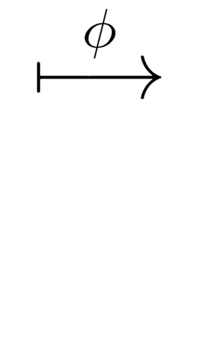
In Figure 4, we can see displayed the antiadjacency matrix of the canonically -labeled unit interval order introduced in Example 1.2 and the matrix both showing their respective semiorder and inverted path encoding the decorated permutation associated to the positroid induced by .
As a consequence of Theorem 5.1, we can deduce that the map , where , , and are as defined in Section 2 and Section 3, is indeed a bijection.
Lemma 5.3.
The set of -cycles satisfying conditions (1) and (2) of Theorem 4.4 is in bijection with the set of Dyck paths of length .
Proof.
We can assign a Dyck path of length to the -cycle by thinking of the entries as ascending steps of the Dyck path and the entries as descending steps of . The fact that such an assignment yields the desired bijection is straightforward. ∎
Theorem 5.4.
The map is a bijection.
Proof.
By definition of , it follows that is surjective. Since is the -th Catalan number, it suffices to show that . To see this, one can take a -cycle satisfying conditions (1) and (2) of Theorem 4.4, and consider the Dyck path specified by as in Lemma 5.3. By Theorem 1.1, the Dyck matrix whose semiorder path is the reverse of induces a unit interval positroid with decorated permutation . Because the decorated permutation associated to a positroid is unique, Lemma 5.3 guarantees that . Hence is bijective. ∎
Corollary 5.5.
The number of unit interval positroids on the ground set equals the -th Catalan number.
We conclude this section by describing how to decode the decorated permutation associated to the unit interval positroid induced by directly from its canonical interval representation . Labeling the left and right endpoints of the intervals by and , respectively, we obtain a -tuple consisting of pluses and minuses by reading from the real line the labels of the endpoints of all such intervals. On the other hand, we can have another plus-minus -tuple if we replace the horizontal and vertical steps of the semiorder path of by and , respectively, and then read it in southeast direction as indicated in the following example.
Example 5.6.
The figure below shows the antiadjacency matrix of the canonically -labeled unit interval order from Example 1.2 and a canonical interval representation of , both encoding the plus-minus -tuple , as described in the previous paragraph.


Lemma 5.7.
Let and be the -tuples with entries in obtained by labeling the steps of the semiorder path of and the endpoints of all intervals in , respectively, in the way described above. Then .
Proof.
Let us proceed by induction on the cardinality of . When , both and are equal to and so . Suppose now that the statement of the lemma is true for every canonically -labeled unit interval order, and assume that is a unit interval order canonically labeled by with antiadjacency matrix and canonical interval representation . Set . By Proposition 3.2, the poset is a unit interval order canonically labeled by ; therefore its associated plus-minus -tuples and are equal. Observe, in addition, that can be recovered from by inserting the corresponding to the left endpoint of (labeled by ) in the position (there are left interval endpoints and right interval endpoints to the left of in ) and adding the corresponding to the right endpoint of (labeled by ) at the end. On the other hand, can be recovered from by inserting the corresponding to the rightmost horizontal step of the semiorder path of in the position (there are horizontal steps and vertical steps before the last horizontal step of the semiorder path) and placing the corresponding to the vertical step labeled by in the last position. Hence , and the lemma follows by induction. ∎
As a consequence of Theorem 5.1 and Lemma 5.7, one obtains a way of reading the decorated permutation associated to the unit interval positroid induced by directly from .
Corollary 5.8.
Labeling the left and right endpoints of the intervals by and , respectively, we obtain the decorated permutation associated to the positroid induced by by reading these labels from right to left on the real line.
Proof.
Example 5.9.
The diagram below illustrates how to label the endpoints of a canonical interval representation of the -labeled unit interval order shown in Figure 1 to obtain the decorated permutation associated to the positroid induced by by reading such labels from the real line (from right to left).

6. The Le-diagram of a Unit Interval Positroid
The set consisting of all -dimensional subspaces of , denoted by , is called the real Grassmannian. Elements in can also be understood as the orbits of the set of full-rank real matrices under the left action of . For and , the Plücker coordinate is the maximal minor of determined by the column set . The embedding induced by the map makes a projective variety. Let denote the set of real matrices of positive determinant, and recall that is the set of real matrices of rank having nonnegative maximal minors.
Definition 6.1.
The totally nonnegative Grassmannian, denoted by , is the set of orbits of under the left action of , i.e., .
For a full-rank real matrix , let denote the matroid represented by , and let denote the element of represented by . The matroid stratification or Gelfand-Serganova stratification of is the collection of all strata
where runs over the set of rank representable matroids on the ground set . For each stratum , we define a positroid cell in by
Note that a representable matroid is a positroid precisely when is nonempty. The collection of nonempty positroid cells is called the cellular decomposition of . For further details, see [12, Sections 2 and 3].
Positroids, and therefore positroid cells, can be parameterized by a family of combinatorial objects called Le-diagrams. In this section, we characterize the Le-diagrams corresponding to unit interval positroids.
Definition 6.2.
Let and let be the Young diagram associated to a given partition . A L -diagram (or Le-diagram) of shape and type is a Young diagram contained in a rectangle, whose boxes are filled with zeros and pluses such that there is no zero entry which has simultaneously a plus entry above it in the same column and a plus entry to its left in the same row.
The left picture in Figure 7 shows a L -diagram of square shape and type . As mentioned before, L -diagrams of type parameterize rank positroids on the ground set . The next lemma yields a method to find the decorated permutation of a positroid given its corresponding L -diagram.
Lemma 6.3.
[2, Lemma 4.8] The following algorithm is a bijection between L -diagrams of type and decorated permutations on letters with weak excedances.
- (1)
Replace each in the L -diagram with an elbow joint
![[Uncaptioned image]](1611.09279v2/LeDiagramElbow.png) , and each in with a cross
, and each in with a cross ![[Uncaptioned image]](1611.09279v2/LeDiagramPlus.png) .
. - (2)
Note that the south and east border of gives rise to a length- path from the northeast corner to the southwest corner of the rectangle. Label the edges of this path with the numbers through .
- (3)
Now label the edges of the north and west border of so that opposite horizontal edges and opposite vertical edges have the same label.
- (4)
View the resulting “pipe dream” as a permutation by following the “pipes” from the northwest border to the southeast border of the Young diagram. If the pipe originating at label ends at the label , we define .
- (5)
If and labels two horizontal (respectively, vertical) edges of , then we set (respectively, ).
The picture on the left of Figure 7 shows the L -diagram corresponding to the positroid induced by the unit interval order displayed in Figure 1. The “pipe dream” of this L -diagram, as described in Lemma 6.3, is depicted on the right.


The next theorem provides a characterization of the L -diagrams corresponding to unit interval positroids.
Theorem 6.4.
A L -diagram of type parameterizes a unit interval positroid on if and only if its shape is a square of size and satisfies the following two conditions:
- (1)
every column has exactly one plus except the last one that has pluses;
- (2)
the horizontal unit steps right below the bottom-most pluses are the horizontal steps of a length Dyck path supported on the main diagonal of .
Proof.
Suppose first that satisfies (1) and (2). To verify that corresponds to a unit interval positroid, let us use Lemma 6.3 to compute its decorated permutation and show that satisfies Proposition 4.3. Note that . For , we find .
Assume first that . If there is only one plus in the -st row of (which means that for each ), it follows by Lemma 6.3 that . On the other hand (which means that there is exactly one principal element in ), one obtains that is the label of the first column (from right to left) of having a plus in the -st row (which means ).
Assume now that . If the bottom-most plus in the column of labeled by is the last plus from right to left in its row, which is labeled by , then by Lemma 6.3 it follows that (note, in this case, that or is a principal index). On the other hand, the columns of labeled by and are identical (i.e., is not a principal index), and Lemma 6.3 yields .
Thus, is as described in Proposition 4.3, and so is the decorated permutation of a unit interval positroid on the ground set . As the number of L -diagrams satisfying the conditions above and the number of decorated permutations corresponding to unit interval positroids on the ground set are equal to the -th Catalan number, the proof follows. ∎
As a result of Theorem 6.4, each unit interval positroid cell in can be indexed by a L -diagrams described in the same theorem. Postnikov proved that the positroid cell indexed by a L -diagram has dimension equal to the number of pluses of [12, Theorem 4.6]. This immediately implies the following corollary.
Corollary 6.5.
The positroid cell of a unit interval positroid on the ground set inside the cell decomposition of has dimension .
7. Adjacency of Unit Interval Positroid Cells
Given a decorated permutation on letters, its chord diagram is constructed in the following way. First, place points labeled by in clockwise order around a circle. For all with and , draw a directed chord from to . If fixes , then draw a directed chord from to , oriented counterclockwise if and only if . For , let denote the set of points in the boundary circle of the chord diagram from to (both included) in clockwise order. Figure 8 shows an example of a chord diagram.

Let and be two chords in the chord diagram of a decorated permutation . We say that and form a crossing if they intersect inside the circle or on its boundary, and this crossing is simple if there are no other chords from to . The left diagram in Figure 9 shows a simple crossing. On the other hand, two chords and form an alignment if they do not intersect and have a parallel orientation as shown in the right diagram of Figure 9. Notice that if and coincided in the right diagram below, then in order for and to have parallel orientation must be a loop oriented counterclockwise. An alignment, as shown in the right side of the picture below, is said to be simple if there are no other chords from to .


Let and be two decorated permutations of the same size . We say that covers , and write , if the chord diagram of is obtained by turning a simple crossing of into a simple alignment. This is depicted in Figure 10.

If the points and happen to coincide, then the chord from to in the chord diagram of degenerates to a counterclockwise loop. Similarly, if the points and coincide, then the chord from to in the chord diagram of becomes a clockwise loop. Finally, if or , then the loops at and in the chord diagram of must be counterclockwise and clockwise, respectively. These three types of covering relations, illustrated in Figure 11, are said to be degenerate.


Two positroid cells are adjacent if the decorated permutation parameterizing them cover a common decorated permutation. Here is a necessary and sufficient condition for two unit interval positroid cells to be adjacent.
Proposition 7.1.
Let and be two distinct rank unit interval positroids and and their respective decorated permutations. Then and label adjacent positroid cells if and only if there exists such that when is removed from the cycle decomposition of and the resulting cycles are equal.
Proof.
Let and be the chord diagrams of and , respectively. Assume first that and label adjacent positroid cells whose decorated permutations both cover a permutation . Let denote the chord diagram of . Theorem 4.4 ensures that and have a directed edge from to and their non-degenerate simple crossings occur only along this edge. Unlike non-degenerate coverings, degenerate coverings increase the number of fixed points; therefore is a degenerate covering relation if and only if so is . If and were both non-degenerate coverings, then the fact that both covering relations uncross the chord from to would imply that both and can be uniquely recovered from , as the other chord being uncrossed in both covering relations must be the chord from to . This, in turn, would contradict that . As a result, both and are degenerate coverings. As and are -cycles, fixes exactly one element . Moreover, is the result of removing from the cycle decomposition of any of the permutations or .
Conversely, suppose that for some , removing from the cycle decomposition of either or produces the same -cycle . In this case, and are degenerate covering relations. Hence and are adjacent and the proof follows. ∎
Example 7.2.
There are a total of five unit interval positroids on the ground set . Let be their five corresponding decorated permutations. These permutations are illustrated in the top row of Figure 12 via their chord diagrams. The bottom row of the same figure shows the chord diagrams of four of the decorated permutations covered by the ’s. Although there are more than four decorated permutations covered by the ’s, those depicted below are enough to obtain all possible adjacency relations between the positroid cells parameterized by the ’s. The exterior long arrows below represent covering relations.

It was proved in [12] that if and are two decorated permutations such that , then they both have the same number of weak excedances. Thus, the set of all decorated permutations of having excedances can be regarded as a poset with order given by the transitive closure of the covering relation “”; this poset is called the cyclic Bruhat order and is denoted by . Given that the adjacency relations of unit interval positroid cells can be described so nicely, we believe the subposet of consisting of those decorated permutations representing positroids in the closures of unit interval positroid cells of may have an interesting description. Here we propose a problem stemming from Proposition 7.1.
Problem 7.3.
Describe the subposet of consisting of those decorated permutations representing positroids in the closures of unit interval positroid cells of .
8. An Interpretation of the -vector of a Unit Interval Order
In hopes of a more thorough understanding of the -vectors of -free posets, Skandera and Reed in [16] posed the following open problem: characterize the -vectors of unit interval orders. In this aim, we provide a combinatorial interpretation for the -vector of a naturally labeled poset in terms of its antiadjacency matrix. Through this section, is assumed to be a naturally labeled poset of cardinality with antiadjacency matrix .
Definition 8.1.
The -vector of is the sequence , where is the number of -element chains of .
We wish to interpret the -element chains of in terms of some special Dyck paths inside . To do this, define a valley Dyck path of to be a Dyck path drawn inside that has its endpoints and all its valleys on the main diagonal and all its peaks in positions such that . The following figure illustrates a valley Dyck path with three peaks.

Proposition 8.2.
The entries of the -vector of are and equals the number of valley Dyck paths of having exactly peaks.
Proof.
To each -element chain we can assign a valley Dyck path with peaks as follows: the -th peak begins at , heads east to , and then heads south to . To see that is a valley Dyck path, it suffices to notice that every peak of occurs at a zero entry of since for each . On the other hand, suppose that is a valley Dyck path with peaks, namely . Then every valley of is supported on the main diagonal, which means that for each . Setting , we obtain that , where is the -element chain . Thus, we have established a bijection that yields the desired result. ∎
Example 8.3.
The naturally labeled poset depicted below has -vector
Examples of valley Dyck paths realized on are also shown below.

| one peak | two peaks | three peaks |
|---|---|---|
 |
 |
 |
Remark: Proposition 8.2 provides, in particular, an interpretation of the -vector of any unit interval order. Given that a unit interval order can be labeled so that its antiadjacency matrix is a Dyck matrix, we think that the interpretation of the -vector in Proposition 8.2 might be useful to find an explicit formula for the ’s. This is because zero and one entries in a Dyck matrix are nicely separated, which could facilitate counting the valley Dyck paths having exactly peaks.
Problem 8.4.
Given an Dyck matrix , let be the number of one entries in the -th row of . For , can we find, in terms of the ’s, an explicit formula for the number of valley Dyck paths of containing exactly peaks?
Acknowledgements
While working on this paper, the first author was partially supported by the NSF Alliances for Graduate Education and the Professoriate, while the second author was partially supported by the UC Berkeley Department of Mathematics. Both authors are grateful to Lauren Williams for her guidance throughout this project, Federico Ardila for many helpful conversations, Alejandro Morales for the initial question that motivated this project, and the anonymous referees for many suggestions that led to an improvement of this paper.
References
- [1] M. Aissen, I. J. Schoenberg, and A. Whitney. On generating functions of totally positive sequences, J. Anal. Math. 2 (1952) 93–103.
- [2] F. Ardila, F. Rincón, and L. K. Williams. Positroids and non-crossing partitions, Trans. Amer. Math. Soc. 368 (2016) 337–363.
- [3] N. Arkani-Hamed, J. Bourjaily, F. Cachazo, A. Goncharov, A. Postnikov, and J. Trnka. Grassmannian Geometry of Scattering Amplitudes. Cambridge University Press, 2016. Preliminary version titled “Scattering Amplitudes and the Positive Grassmannian” on the arXiv at http://arxiv.org/abs/1212.5605.
- [4] W. E. Armstrong. The determinateness of the utility function, Econ. J. 49 (1939) 453–467.
- [5] R. A. Dean and G. Keller. Natural partial orders, Canad. J. Math. 20 (1968) 535–554.
- [6] P. C. Fishburn. Interval Graphs and Interval Orders, Wiley, New York, 1985.
- [7] P. C. Fishburn. Interval representations for interval orders and semiorders, J. Math. Psych. 10 (1973) 91–105.
- [8] P. C. Fishburn and B. Monjardet. Norbert Wiener on the theory of measurement (1914, 1915, 1921), J. Math. Psych. 36 (1992) 165–184.
- [9] Y. Kodama and L. K. Williams. KP solitons and total positivity on the Grassmannian, Invent. Math. 198 (2014) 637–699.
- [10] R. D. Luce. Semiorders and a theory of utility discrimination, Econometrica 24 (1956) 178–191.
- [11] S. Oh. Positroids and Schubert matroids, J. Combin. Theory Ser. A 118 (2011) 2426–2435.
- [12] A. Postnikov. Total positivity, Grassmannians, and networks, on the arXiv at https://arxiv.org/abs/math/0609764.
- [13] D. Scott. Measurement structures and linear inequalities, J. Math. Psych. 1 (1964) 233–247.
- [14] D. Scott and P. Suppes. Foundational aspects of theories of measurements, J. Symbol. Logic 23 (1958) 113–128.
- [15] J. S. Scott. Grassmannians and cluster algebras, Proc. London Math. Soc. 92 (2006) 345–380.
- [16] M. Skandera and B. Reed. Total nonnegativity and (3+1)-free posets, J. Combin. Theory Ser. A 103 (2003), 237–256.
- [17] W. T. Trotter. Combinatorics and Partially Ordered Sets: Dimension Theory, Johns Hopkins University Press, Baltimore, 1992.
- [18] N. Wiener. A contribution to the theory of relative position, Proc. Cambridge Philos. Soc. 17 (1914) 441–449.
- [19] R. L. Wine and J. E. Freund. On the enumeration of decision patterns involving means, Ann. Math. Stat. 28 (1957) 256–259.