Nonabelian Higgs models: paving the way for asymptotic freedom
Abstract
Asymptotically free renormalization group trajectories can be constructed in nonabelian Higgs models with the aid of generalized boundary conditions imposed on the renormalized action. We detail this construction within the languages of simple low-order perturbation theory, effective field theory, as well as modern functional renormalization group equations. We construct a family of explicit scaling solutions using a controlled weak-coupling expansion in the ultraviolet, and obtain a standard Wilsonian RG relevance classification of perturbations about scaling solutions. We obtain global information about the quasi-fixed function for the scalar potential by means of analytic asymptotic expansions and numerical shooting methods. Further analytical evidence for such asymptotically free theories is provided in the large- limit. We estimate the long-range properties of these theories, and identify initial/boundary conditions giving rise to a conventional Higgs phase.
I Introduction
A fascinating aspect of quantum field theories is the fact that they can represent truly fundamental theories valid on all energy or length scales as a matter of principle – or predict their own failure. An example of the first class are nonabelian gauge theories that represent perfect quantum field theories in the sense of being potentially valid on all scales. In particular, their high-energy behavior is governed by asymptotic freedom [1, 2]. This property persists also upon the inclusion of a suitable matter content [3, 4, 5, 6, 7, 8].
An example of the second class are pure scalar theories in spacetime dimensions which suffer from triviality [9], implying that a meaningful continuum theory exists only for the noninteracting theory. While rigorous proofs for triviality exist for [10], strong evidence for triviality in has been collected by lattice simulations [11, 12, 13, 14, 15, 16, 17] as well as by functional renormalization group (RG) studies [18]. Similar conclusions appear to hold for QED [19, 20].
While triviality rather represents a mathematical consequence that arises from insisting on sending the maximum validity scale of a theory (technically corresponding to an ultraviolet (UV) cutoff) to infinity, the physical viewpoint is slightly different: by keeping the interaction at low energies finite, triviality translates into a breakdown of the quantum-field-theory description at a finite UV scale. For instance, in perturbation theory this is signaled by the artifact of a Landau pole singularity in the RG evolution of couplings [21, 22]. Nonperturbatively, this singularity might be screened such as in QED [19, 20], but the conclusion persists that the physically observed infrared (IR) behavior cannot be connected to the same theory at an arbitrarily high scale with suitably renormalized couplings.
Triviality appears to threaten the standard model of particle physics not only with respect to its U(1) sector. It is well conceivable that the U(1) factor arises from symmetry breaking of a compact grand unified gauge theory. It is rather the potential triviality of the Higgs sector which we consider as the more substantial obstacle of building a perfect quantum field theory for particle physics. Hence, we concentrate on nonabelian Higgs systems in the present work.
A naive expectation would be that nonabelian Higgs systems should be trivial, as the gauge sector is asymptotically free such that the scalar triviality problem remains. This is not necessarily true: already a standard perturbative analysis [3, 23, 24, 25, 26, 27, 8, 28, 29] reveals the existence of gauged Yukawa models, where also the seemingly problematic scalar self-interaction can become asymptotically free as well. This happens along suitable RG trajectories depending on the precise matter content of the model. Such scenarios in principle have the advantage of yielding a reduction of couplings [30, 31, 32], as the scalar self-interaction may then be induced by the gauge sector. In essence, this can fix the Higgs-to-gauge-boson mass ratio. So far, a concrete model building has not been satisfactory, as no unequivocally convincing model sufficiently similar to the standard model has been identified, though the search is ongoing, see, e.g., [33, 34, 35, 36].
In the present work, we detail and extend our recent results on the construction of asymptotically free non-abelian Higgs models which become visible upon the use of generalized boundary conditions for the correlation functions of the theory [37]. The fact that the RG behavior of a model is sensitive to boundary conditions is well known from interacting fixed-points in statistical field theories. For instance, the scaling solution for the potential at the Wilson-Fisher fixed point yields the correct critical exponents of the Ising universality class, once it satisfies suitable boundary conditions for small and large fields as well as self-similarity conditions [38, 39, 40, 41]. The new ingredient in our construction is that we allow for boundary conditions for the scalar potential which depend on the gauge coupling .
Such a dependence appears natural in view of the fact that the scalar potential governing the scalar self-interactions is expected to become absolutely flat for an asymptotically free theory, vanishing synchronously with the asymptotically free gauge coupling . In contrast to the role of boundary conditions at interacting fixed points, which typically constrain the number of possible scaling solutions severely (see, e.g., the singularity count in [42, 43]), we find a larger set of possibilities of imposing boundary conditions on the scalar potential in the case of asymptotic freedom, yielding a family of scaling solutions.
The present work intends to give a detailed account of our construction. For this, we use several approaches of increasing sophistication in order to explain our results from various viewpoints. In Sect. II, we start from simple one-loop perturbation theory in order to make contact with the standard language of describing asymptotic freedom. Sections III and IV use the language of effective field theory that allows to study the renormalization properties of the model upon the inclusion of higher-dimensional operators. This approach makes the asymptotically free scaling solutions already visible and facilitates a first glance at their connection to RG boundary conditions. In Sect. V, the picture unfolds more comprehensively on the basis of the functional RG flow of nonabelian Higgs models. This modern tool gives access to the global behavior of the scalar potential at high energies and allows for a classification of the scaling solutions as well as a RG relevance count of perturbations about the noninteracting Gaußian fixed point. Further insights are obtained on the basis of a large- approximation in Sect. V.5.3, which also allows for a first but rough estimate of the full flow from the UV to the IR. The latter is also discussed more phenomenologically in Sect. VI in order to estimate the long-range properties of our models. We conclude in Sect. VII.
II Perturbative one-loop analysis
We consider nonabelian Higgs models with an SU() gauge sector coupled to a charged scalar in the fundamental representation. The classical action reads
| (1) |
where . Classically, the model has three (bare) parameters, the scalar mass , self-coupling , and gauge coupling . From a perturbative viewpoint, the two couplings correspond to deformations of the free theory. The noninteracting limit denotes the Gaußian fixed point. The covariant derivative reads
| (2) |
where are the generators of the fundamental representation and denotes the Yang-Mills vector potential with field strength .
For the present purpose, perturbative quantization of the model is most-conveniently performed with the Faddeev-Popov method applied to a background-field gauge, as detailed below in Sect. V. For a first perturbative glance at the system, it suffices to consider the conventional one-loop functions for the renormalized couplings and , as presented for example by Gross and Wilczek [3],
| (3) | |||||
| (4) |
where denotes the derivative with respect to an RG scale . The constants are given by
| (5) | |||||
We mostly specialize to the simplest case of SU(2), where
| (6) |
We emphasize that these functions approximate perturbatively the RG flow of the couplings in the deep Euclidean region, where all mass scales are neglected compared to energy, momentum, or RG scales. In this regime, the flow of the mass parameter decouples from Eqs. (3),(4), and is thus ignored at this point. The functions define a vector field on the coupling space. The zeros of this vector field read
| (7) |
The notation suggests that the Gaußian fixed point can be read as being governed by the vanishing of the gauge coupling . At finite , the constant combinations define the zeros of the scalar sector, . For SU(2), these roots are complex,
| (8) |
(they turn real for ). In the present simple case, the RG flow can be integrated straightforwardly. The flow of can be written as
| (9) |
where
| (10) |
and is an integration constant. The flow of the gauge coupling obeys the standard asymptotically free log-like running involving a separate integration constant.
If were positive, one could follow a smooth trajectory in the positive plane down to the origin corresponding to the Gaußian fixed point, and the theory would be asymptotically free. However, since is negative for all SU() with , the turns into a tangent. This induces branch cuts at positions depending on the initial conditions. One cut inevitably occurs in between a positive initial point and the origin. This is the nonabelian Higgs version of the Landau pole occurring in the pure scalar theory that prevents the theory to be perturbatively meaningful at all scales. This is plotted for the present model in the left panel of Fig. 1.


Incidentally, could be made positive by suitably tuning to small values upon introducing a balanced number of fermions. This line of model building has been pursued since the early days of asymptotic freedom [3, 23, 24, 25, 26, 27, 8, 28, 29]. However in this work, we stay within the class of nonabelian Higgs models, and intend to construct asymptotically free trajectories without further degrees of freedom.
The perturbative Landau-pole problem can also be illustrated directly with the RG flow vector field provided by the functions on the plane. Such a phase diagram is shown in the right panel of Fig. 1. The branch cut manifests itself in the form of a separatrix making its way from the lower right corner of the plane to the origin. Trajectories starting at at an IR scale are repelled from this separatrix during their flow towards the UV (direction of arrows) and run away towards in a finite RG time. Trajectories on the left of this line at positive but negative are on the left of their own Landau pole and approach the Gaußian fixed point in the UV. The latter trajectories are considered unphysical as the scalar potential appears unstable.
As emphasized above, the existence of this Landau-pole behavior of perturbation theory is tied to the fact that for the present model. In order to illustrate the expected UV behavior for asymptotically free theories, let us discuss a fake model with positive for the remainder of the section. For this, we simply change the sign of by hand. As mentioned above, there is no Landau pole in this case which also becomes obvious in the streamplot in the left panel of Fig. 2. As a consequence of the negative sign of implying , the trajectories that satisfy physical boundary conditions with positive in the IR are now asymptotically attracted by the Gaußian fixed point towards the UV, and no run-away to occurs.


In the left panel of Fig. 2, we highlight two lines that correspond to the trajectories with
| (11) |
which can be obtained in the limit or , respectively. Along these trajectories, the system shows a peculiar behavior since is proportional to at all scales. Eq. 9 shows that all the asymptotically free trajectories of this model close to the Gaußian fixed point have a leading linear -dependence with a -independent proportionality constant ; i.e., all trajectories exhibit the same UV asymptotics for . This is in agreement with the observation that zeros of need to be of order , but it might be surprising that the constant of proportionality does not agree with these zeros, cf. Eq. (7). The mismatch has a deep meaning and is of key relevance for what follows.
In a one-loop set-up, asymptotic freedom occurs with an asymptotic scaling of proportional to . The latter piece of information can be encoded in the condition that the ratio is frozen in the far UV, namely that [3]. Since
| (12) |
we can understand the above-mentioned mismatch by realizing that is the relevant condition that characterizes all the asymptotically free trajectories, rather than simply (which is nevertheless satisfied at ). Thus, one can translate the flow diagram of the model in terms of , as in the right panel of Fig. 2. This makes the properties of the asymptotically free trajectories more transparent. We observe that the flow of has two fixed points corresponding to at finite with different properties. For , the -direction is UV attractive (RG relevant), implying that we can build a one-parameter family of trajectories hitting this fixed point. For , the -direction is UV repulsive (RG irrelevant), such that only one trajectory hits this fixed point. This trajectory is obtained by moving off this fixed point along the marginally relevant direction , without switching on any component along the -direction. This trajectory is an example of a reduced number of physical parameters for the IR physics (in the present fake model, however, it corresponds to unphysical negative values of the coupling ).
In conclusion, the roots of the finite- fixed-point equation for classify the asymptotic (small ) behavior of the possible asymptotically free trajectories. The latter trajectories exist in the real space of couplings if and only if there are real roots of . These roots are a first example for the auxiliary concept of quasi-fixed points, which is heavily used below: such quasi-fixed points denote zeroes of the functions of the appropriately -rescaled scalar sector even for finite values of the gauge coupling . Incidentally, this fixed point condition for ratios of couplings, has been used in the literature for a long time, starting with [3], under different names, such as eigenvalue conditions [23] [8] or fixed-flows [28]. As a seemingly trivial consequence of the shift from to , we have for any for vanishing gauge coupling . In other words, the Gaußian fixed point , in the old parametrization, becomes the whole axis in the new parametrization. This trivial statement has an immediate consequence for the search for nonvanishing- fixed-points. Whereas the standard parametrization demands for a trajectory hitting a single point in the far UV, the new parametrization requires to search for trajectories hitting a whole axis. In the fake model and within the one-loop flows discussed above, trajectories exist that asymptotically reach one of two possible points on the -axis.
III Effective field-theory analysis in the deep Euclidean region
The previous standard one-loop analysis of the nonabelian Higgs model (with the correct positive sign for ) reveals the absence of perturbative asymptotic freedom. This result clearly holds under the standard assumptions for a perturbative analysis, being typically extendible to any finite order in an expansion in terms of . Further implicit assumptions include, for instance, the anticipated appropriateness of an analysis in the deep Euclidean region, such that the running of mass terms and threshold effects can be ignored.
Despite the seemingly negative answer from the perturbative analysis of the real model, we keep the lesson from the fake model in mind that asymptotically free trajectories – if they exist – can be characterized by a peculiar kind of scaling, for which the scalar self-interactions are governed not only by the renormalization scale but also by the running gauge coupling. For the correspondingly rescaled coupling , the Gaußian fixed point unfolds to a whole line which may or may not be reachable by legitimate RG trajectories.
Let us now slightly change the viewpoint: considering the interaction term , we can also reinterpret the coupling rescaling as a field rescaling
| (13) |
Now, if happens to approach the line for on an asymptotically free trajectory (as in the fake model), fluctuations of the rescaled field variable will correspond to large amplitude fluctuations in . This motivates to go beyond the lowest-order interaction term and more generally study the full running potential. In the spirit of effective field-theory, we can span the full potential in terms of operators of increasing mass dimension,
| (14) |
where the couplings are dimensionless because of an appropriate scaling with the RG scale , and labels the highest order included in this operator expansion. For simplicity, we ignore here the necessary wave function renormalizations for the proper definition of the renormalized couplings. They are included in the full calculation and will be more carefully introduced in the next section.
In standard effective field theory, a potential as in Eq. (14) or further higher-dimensional operators are used to parametrize the physics at a fixed (high-energy) scale , and then fluctuations are integrated out to describe the long-range physics at momenta . In the present work, we instead use Eq. (14) with the running scale and study the flow of the couplings towards higher and higher energies.
In this spirit, each coupling has its own RG flow given by the corresponding function, which can be derived by standard effective-field theory techniques (see also next section). In the massive scheme and within the approximations considered in this work, the function generically depends on the couplings up to order ; (precise definitions will be given in Sec. V). Truncating the expansion in Eq. (14) as well as the set of functions at a fixed polynomial order , leaves the next higher coupling undetermined, even though it enters the flow equation for . To close the system of equations, one may approximate . This is well justified in a perturbative region where the higher-order operators are generated by the fluctuations involving the leading operators, and hence parametrizes subleading higher-loop corrections.
While Eq. (14) is a suitable expansion in the symmetric regime, the potential can also be expanded about the vacuum expectation value in the broken regime,
| (15) |
The mass-like parameters of Eq. (14), or in Eq. (15) are assumed to be negligible for a UV analysis in the deep Euclidean region. In fact, the validity of this assumption has been challenged in a series of works [44, 45, 46], where nontrivial RG flows towards the UV have been constructed on the basis of scale-dependent threshold phenomena. The present work is partly related with these constructions, but more generally relates the new UV trajectories to boundary conditions at large fields, allowing for asymptotically free scaling solutions.
III.1 First glance at scaling solutions
In order to understand how the higher-dimensional perturbatively non-renormalizable operators in Eq. (14) can support the construction of asymptotically free scaling solutions, let us generalize the concept of rescaling the scalar coupling or fields by the gauge coupling, cf. Eq. (13), to the full potential. By consistency, this entails consequent rescalings of higher polynomial couplings, . Yet, might still attain vanishing or diverging values towards the UV.
The presence of fixed-points (in the fake model) at for finite values of now serves as a motivation for a new search strategy for asymptotically free trajectories. As a hypothesis, let us for the moment assume that the model beyond the perturbative realm admits trajectories hitting any chosen point along the asymptotically free axis. If this were the case, neither perturbation theory nor truncations of the effective-field theory expansion at a fixed setting would be able to reveal this feature: there simply is no free parameter in the remaining set of functions that would allow us to choose the value at which the flow arrives in the UV.
In order to test this hypothesis, we need an approximation that is able to describe lines of fixed points, i.e. allowing for the presence of a free parameter. This can be achieved in the effective-field theory context by treating the next coupling outside a given truncation as a free parameter instead of assuming that it can be ignored. From the point of view of a full functional approach discussed in the next section, where we deal with the full potential and not with simple polynomials, this free parameter can be interpreted as emerging from the boundary conditions for the potential.
Let us now demonstrate in a somewhat oversimplified setting, that such a parameter freedom can be sufficient to find trajectories that reach any desired value for in the far UV. For this, we consider the one-loop flow within the effective-theory approach and minimally include the coupling as a free parameter, corresponding to truncating at . Staying within the deep Euclidean region (), the function for , or alternatively reads,
| (16) | |||||
| (17) |
As does not represent a power-counting renormalizable coupling, the coefficient is non-universal, i.e., scheme and regulator dependent. In our scheme detailed below and for SU(2), we have . All other constants are the same as in Sect. II.
Having as a free parameter in Eq. (17) is equivalent to a free coefficient in the pure one-loop case. As a consequence, we can choose such that the roots are real. Specifically, the inclusion of in Eq. (17) amounts to replacing in Eq. (12) with . This suggests to keep the ratio fixed, such that approaches finite real roots in the limit,
| (18) |
representing quasi-fixed points, where
| (19) |
The integrated flow is then again
| (20) |
where is an integration constant. For chosen such that , there is no Landau pole in . Hence, we obtain asymptotically free trajectories, as can be seen from Fig. 3.


We observe that the fixed point for a given ratio with a positive value of for has a marginal-irrelevant direction, implying that the long-range physics depends on one physical parameter less then predicted by perturbative power counting. This dynamical reduction of parameters is, however, compensated by the necessary choice of a value for . Nevertheless, the meaning of these parameters has slightly changed: whereas in the perturbative framework we fix parameters within a theory, different values of correspond to different boundary conditions and thus rather to different theories.
At this simple stage, the choice of fixing to a constant looks rather arbitrary. In particular, it implies that we are fixing specific dependencies for the couplings, e.g., or . A gauge coupling dependence is only natural as the gauge sector will inevitably drive the running of higher-order operators. Still, at this simple level of approximation, it seems that we would have to guess the correct scaling of couplings in the full system or we are left with an ambiguity of possible different choices. In the next section, we demonstrate that this ambiguity is removed in the full system leading to a remaining dependence on the boundary conditions for the theory.
To illustrate the effect of different choices in the present simple setting, let us insist on a flow that keeps constant at the expense of choosing (or ) accordingly. Insisting on as a function of and , leads us to a flow of given by
| (21) |
To lowest order in the gauge coupling, we obtain
| (22) |
Again, we observe the existence of quasi-fixed points at finite , satisfying the same relations (18) and (19), including the implicit mapping between a choice for and the corresponding value of . The corresponding flow at a fixed is shown in Fig. 4. We conclude that the asymptotic properties of these asymptotically free trajectories are independent of the precise choice of the free parameter. For both choices of finite asymptotic ratios or we observe asymptotic freedom and a UV fixed-point behavior with the same type of marginal-irrelevant perturbation in the mutual dynamical coupling or , respectively.

III.2 Generalized scaling solutions
The preceding simple analysis revealed that an appropriate scaling of the higher-order operators is required in order to build asymptotically free trajectories. At a first glance, it seems that the scaling for small is essential for the desired result. For instance, if we keep constant, the last term in Eq. (17) makes diverge towards the UV. Still, for an answer about the (non-)existence of asymptotically free trajectories in that case, we have to inspect the UV flow of .
In order to understand the set of possible consistent scalings that feature asymptotically free trajectories, let us try to generalize the previous analysis. For this, we start from the function (16) in the effective-theory setting with as before, keeping as a possibly scale-dependent free parameter. As before, we assume to be finite, and look for quasi-fixed points defined by . For , we precisely discover the one-parameter family of the preceding subsection parametrized by a fixed value of .
Let us now be more general and set
| (23) |
(in this language, the value corresponds to the previous analysis). The quasi-fixed points of are then given by the analogue of Eq. (18) with the replacement
| (24) |
For , the term dominates in the small-coupling limit, yielding real roots,
| (25) |
For fixed , we hence observe a whole set of further asymptotically free trajectories parametrized by the power . At this point, it seems that has to satisfy , since the term vanishes for small gauge coupling for and the corresponding roots in remain complex. In the following, we use the terminology -scaling solutions for the asymptotically free trajectories where vanishes proportional to in the UV (in the present case, we have for ; as shown below, the counterparts, in fact, do exist, but only become visible, once we drop the artificial restriction to the deep Euclidean regime). That or could scale like some arbitrary non-integer power of might look suspicious, and might point to possible pathological properties of these trajectories. Nevertheless, our analysis, as discussed more in detail in what follows, is not able to rule out this possibility. Moreover, such kind of asymptotically free trajectories have already been discovered at one loop in supersymmetric models [47][48], see also [31] for a lucid explanation close to the present treatment.
Let us look at the case more specifically using the example mentioned above where approaches a constant. In the new notation of Eqs. (23) and (25), this corresponds to the case and . From Eq. (25), we expect the occurrence of asymptotically free trajectories where vanishes like in the UV. These trajectories can indeed be localized in the phase diagram in Fig. 5 (upper panel). From the perspective that the rescaling with the gauge coupling corresponds to a rescaling of the fields analogously to Eq. (13), , it is useful to also generalize the definition of the the gauge-rescaled couplings:
| (26) |
With this generalized definition, the asymptotically free trajectories become again manifest by ending on the axis in the plane, with for , see Fig. 5 (lower panel).


Again, there is a trajectory reaching a positive fixed point with a marginally-irrelevant direction. The new feature for the present case is that the critical trajectory emanating from this fixed point is no longer independent. In order to verify whether a given point in the coupling plane in the IR is on the asymptotically safe trajectory, we have to integrate the flow towards the UV (with sufficient numerical precision). The explicit trajectories (blue curves) in the plane (upper panel) or plane (lower panel) are shown in Fig. 6. We also plot the positive root of the equation , i.e. the quasi-fixed point, for any given value of (black curves) which represents a reasonable approximation for small values of the gauge coupling. Though the quasi-fixed points (determined as a function of ) do not give the correct physical RG flow, the results of Fig. 6 demonstrate that the quasi-fixed points can be used to track or approximate scaling solutions of the full system in the asymptotically free regime .


The results are similar for any other value of the scaling power . If we consider the effective-field-theory flow equations at fixed , we can build asymptotically free trajectories such that the rescaled coupling attains a finite positive value in the limit. Any limiting value of can be reached by a suitable choice of . For small the corresponding trajectory can be approximated by the quasi-fixed point given by the positive root of the equation . Explicitly,
| (27) |
with the generalized definition,
The resulting quasi-fixed-point representing an approximation to the flow trajectory for small is then
| (28) |
Some of these are plotted in terms of for different values of in Fig. 7.

A natural question is, of course, whether the present simplest approximation of the effective-field theory RG flows truncating at is legitimate and capable of describing the full system appropriately. In fact, it is straightforward to generalize the argument to any higher by self-consistently solving the coupled system of flows for and choosing an appropriate -dependent scaling for the highest order occurring in the flows. The result is a polynomial approximation to a full scalar interaction potential which approaches asymptotic flatness on a suitable trajectory in the limit .
Since all couplings scale with certain powers of to zero, one may actually worry about the influence of , which according to Eq. (26) scales with the least power of . So far, we have ignored possible contributions by assuming that it suffices to stay within the deep Euclidean region. A more careful discussion is the subject of the following section.
IV Effective field-theory analysis including thresholds
Let us now give up the artificial restriction to stay within the deep Euclidean region. In standard analyses, this region where all momenta and RG scales are assumed to be larger than any mass scale is used to define RG functions such as the functions. Together with the use of a mass-independent RG scheme, this removes any mass-scale dependence from the RG functions. As long as these mass-scales do not run fast or grow large in the UV, the analyses in the deep Euclidean region suffices completely to study the UV properties of a theory also in the broken phase [49]. In fact, some of our scaling solutions turn out to violate the implicit assumptions underlying the deep Euclidean analysis. Hence, we now include mass scales that can induce threshold behavior explicitly in our simplified effective field-theory analysis in the following.
The deviations from the deep Euclidean behavior show up in the behavior of the scalar expectation value . Therefore, we concentrate on the expansion (15) which to lowest order as required for the approximation reads
| (29) |
In addition to the RG flow of , we also consider the flow of or a suitably gauge-rescaled version thereof. Apart from possible wave function renormalizations, the gauge/field rescaling suggests to consider the dimensionless variable
| (30) |
with denoting the dimensionless expectation value without gauge rescaling. If or is nonzero, the gauge and scalar propagators acquire mass terms which are also accounted for in the following. Since does not correspond to a marginal operator, its flow is not universal, but scheme and regularization dependent. Throughout this work, we use a natural functional RG scheme, the details of which are given below in Sect. V. Here we continue with the simplified effective field-theory-type analysis in the spirit of the preceding section.
IV.1 -scaling solutions
Let us start by analyzing the role of the flow of the scalar expectation value for the example , where the analysis in the deep Euclidean region revealed a scaling solution with for a fixed . We are specifically interested in the role of the rescaled expectation value . To one-loop order, we obtain the following flow equations to lowest order in the gauge coupling
| (31) | |||||
The equation exactly corresponds to Eq. (22), except for the last term, which arises from the fact that the potential is expanded about the running expectation value . (Here and in the following, the functions can be obtained by straightforward expansion of the full RG flow of the potential given below in Eq. (71), taking the gauge rescalings appropriately into account.)
We observe again that Eqs. (31) and () exhibit quasi-fixed points at finite values of . For instance those of can be read off by plotting the required value of for a given value of in order to obtain , see Fig. 8 .

As a new feature, we observe that also negative values of can lead to admissible values of . Naively, a negative seems to indicate that the potential may become unstable towards large field amplitudes. However, the sign of the highest term in a truncated expansion does not necessarily capture the global stability properties. All global solutions given below are fully stable. The important observation at this point is that an asymptotically free trajectory appears to exist for any value of which can be constructed with a suitable choice of fixed .
Once, the quasi-fixed-point value for has been identified, Eq. (31) yields the corresponding quasi-fixed-point value for , which is approached in the UV in the limit . These values are shown in Fig. 9 as a function of for fixed (upper panel), or as a function of for (lower panel). In particular, this lower panel shows that does not vanish in the deep UV, but approaches a constant. This implies that the dimensionful expectation value of the field increases with the scale towards the UV, for . In other words, the RG flow is never in the deep Euclidean region along this asymptotically free trajectory.


As the inclusion of goes along with an operator , we have now included a power-counting relevant direction in the flow. It is straightforward to verify that this also holds for our approach to the asymptotically free fixed point. In Fig. 10, we show the flow in the plane at fixed values of . The single green (critical) line in Fig. 3 has become a two-dimensional surface (a line in each slice of Fig. 10), i.e. a one-parameter family of trajectories. In other words, the UV critical surface of each UV fixed point becomes two-dimensional, and any point on this trajectory lies on top of an asymptotically free trajectory.


This is consistent with power-counting Gaußian critical exponents, which suggest that the UV critical surface can be parametrized by and . This can be verified by computing the critical exponents (scaling dimensions) within the present approximation of the beta functions from a linearization near the Gaußian fixed point. Collecting the couplings in a vector with components , we consider the stability matrix
| (33) |
at the fixed point . The critical exponents correspond to minus the eigenvalues of this matrix. This linearization has to be done with care by using the coupling instead of , otherwise we would run into an artificial branch-cut singularity at vanishing . Furthermore, we use and as couplings, and parametrize the set of trajectories with the UV fixed-point value for for . The standard diagonalization of the stability matrix then leads to the expected Gaußian set of exponents and perturbations, that is, to the following eigenvalues and eigenvectors of the linearized flow
| (34) |
The first line characterizes the relevant direction corresponding to a scalar mass term with in agreement with the power-counting dimension. The second line refers to the quartic coupling, which is marginal at the linear level as usual; as discussed below, nonlinearities of the flow make it, in fact, marginally irrelevant. The second vanishing exponent in the third line corresponds to the marginally relevant direction due to the function of the gauge coupling. Notice that in presence of scalar degrees of freedom this direction necessarily mixes the gauge and the scalar sector, since gauge loops induce scalar self-interactions. The UV value for parametrizes this set of marginally relevant directions corresponding to asymptotically free trajectories ending at for . The fact that the UV critical surface is spanned by a relevant coupling, which for decreases as , and a marginally relevant coupling, which shows a log decrease , entails that all the asymptotically free trajectories merge into a single trajectory for very large RG time. This single trajectory is characterized by a vanishing relevant component and, as a consequence, it approaches the Gaußian fixed point with a vanishing critical exponent .
The trajectory asymptotically approaching a given value of can be constructed in the same way as before this time including the parameter . Concentrating on the case, where does not flow rapidly, we consider values, where , i.e., near the glitches in Fig. 10. From the first line of Eq. (31), we can solve for as a function of and , thus reducing the problem to a two-dimensional theory space. The leading order of the beta-function of as displayed in Eq. () does not depend on , such that this reduction leaves the far UV running of the quartic coupling unaltered. We plot the corresponding projection of the RG vector field in Fig. 11.

As we had before for the case without a relevant direction, cf. Fig. 3 (right panel), the asymptotically free trajectory is simply parametrized by a constant value of . This is exactly the one corresponding to the quasi-fixed points of Eq. () at nonvanishing .
We anticipated that the quartic coupling is marginally irrelevant, but this issue needs a careful analysis, since it reveals some subtleties. To this end, one can inspect the eigenvalues of the stability matrix up to order ,
Here we set and to their relative quasi-fixed-point values, but keep nonvanishing. While and are always positive, the sign of can change depending on . Inserting the determination of in terms of at the quasi-fixed point one finds
| (35) |
Hence, is negative everywhere apart for the region to the right of the pole in Fig. 8, where the curve has negative slope. In other words, the quartic coupling is always irrelevant apart for the latter case. This region of values can be achieved by fixing to a sufficiently positive number, cf. Fig. 8. If this is the case, there is always one additional quasi-fixed point at which the quartic coupling is irrelevant.
These quasi-fixed points should manifest themselves as two asymptotically free trajectories, a UV stable one, at a smaller value of , and a UV unstable one, at a bigger value of . At the leading order of Eq. (), these trajectories are straight lines. Both at next and next-to-next-to-leading order in (NLO and NNLO in the following) these trajectories become curves which move towards negative values of , possibly merging at some finite value of . The corresponding stream plots look essentially identical at NLO and NNLO, therefore we show the NLO one in Fig. 12. Also the value of at which moves towards zero is essentially the same. We conclude that this remains true also at higher orders. Let us recall that we need to replace by its quasi-fixed-point value to produce these plots; this value can be computed analytically not only at leading order Eq. (), but also at NLO and at NNLO. By sampling other large positive values of , we always observe the same phenomenon, which makes us believe that the branch of quasi-fixed-point solutions having are generically affected by an instability driving the quartic coupling towards negative values. The remaining branch of quasi-fixed-point solutions, at which the quartic coupling is marginally irrelevant, does not show such a behavior, and the potential remains stable at every . For this reason, we will address only such solutions in what follows.


It is instructive to compare the present trajectories to those considered by Coleman and Weinberg in the context of scalar QED [50]. The Coleman-Weinberg (CW) trajectories are characterized by renormalization conditions that ensure the absence of a bare and renormalized scalar mass parameter. In the present setting, this is equivalent to demanding for the absence of a relevant component at any scale, which can here be arranged for without spoiling asymptotic freedom. Whereas a nontrivial vacuum expectation value is generated along CW trajectories towards the IR, the present marginally relevant asymptotically free trajectory exhibits a finite value of the scale dependent potential minimum at and close to the UV fixed point. For increasing towards the IR we observe the same property, at least approximately by recalling that the line of fixed points at nonvanishing , plotted in Fig. 9, is a satisfactory approximation of the asymptotically free trajectories for sufficiently small . The main difference to the CW trajectories is that our trajectories are asymptotically free and do not suffer from UV Landau poles. In this sense the present trajectories are similar to those considered by Salam and collaborators [26] where the UV behavior is also characterized by a vanishing quartic coupling . Unlike in the CW mechanism, the absence of a relevant component at an initial renormalization scale does not entail that the bare Lagrangian is classically scale invariant. Indeed it is not, since is always nonvanishing. Only asymptotically at full (not classical) scale invariance is recovered.
Another important difference is that the present case actually offers a one-parameter family of marginally-relevant asymptotically free trajectories labeled, e.g., by the value of at the fixed point. This free parameter does not occur in the original CW mechanism since the free quartic coupling is unambiguously tied to the gauge coupling in order to reach the symmetry-broken phase. As a consequence, the ratio between the Higgs mass and the gauge boson mass can be predicted along CW trajectories, being a fixed number. While the CW trajectories are conceptually attractive as they do not suffer from a naturalness problem, they seem not relevant for standard-model phenomenology, as this mass ratio unfortunately comes out too small for accommodating the Higgs and boson masses. For our marginally-relevant asymptotically free trajectories, the existence of a one-parameter family of trajectories implies that the mass ratio of scalar and gauge boson masses becomes a function of the free parameter . This means, our scenario features marginally-relevant asymptotically free trajectories with zero relevant direction (“CW-like”) apparently free from a naturalness problem, as the relevant direction corresponding to the field expectation value does not run quadratically with the RG scale . Hence,it is interesting to estimate the IR mass spectrum emerging from these trajectories. For this, we study the flow of the dimensionful mass parameters
| (36) |
This ratio is at any scale equal to evaluated at that scale, and the latter strongly depends on its fixed-point value at , which is an arbitrary positive number. Plots of this ratio are given below within a full FRG analysis. However, these are restricted to the case of standard trajectories featuring a IR Higgs phase thanks to the presence of a nonvanishing relevant component. As far as CW trajectories in their original sense are concerned, the task of following their flow over many orders of magnitude while consistently eliminating the relevant component and possibly capturing strongly-coupled dynamics, is beyond the reach of the present work.
To summarize, an effective-field theory treatment including a parametrization of the influence of higher-dimensional operators by one free parameter allows to construct a two dimensional UV critical surface for each fixed point with positive . This translates into a -dimensional family of asymptotically free trajectories, that can be labeled by the free parameter , which in turn can be expressed in terms of in the far UV, or by the relevant component at a finite value of . It is tempting to view as an exactly marginal coupling, parametrizing a line of fixed points. However, parametrizes different boundary conditions for the RG flow. Thus, different values of can rather be considered as parametrizing different theories.
IV.2 -scaling solutions
For the discovery of asymptotically free trajectories in the effective-field-theory setting discussed above, it is crucial to introduce a parametrization of the influence of unknown higher-dimensional operators. Still, the UV behavior has remained accessible by standard perturbative expansion techniques with the gauge coupling as the governing small parameter. For the details of the expansion, it is important to keep track of the dependence of the boundary condition, which is parametrized by the rescaling power in our setting.
We are therefore looking for the simplest description that preserves the presence of real finite- quasi-fixed points, at values of the coupling that come arbitrarily close to the full description in the limit. In the previous subsection, this simplest description for is provided by the next-to-leading dependence of and . The corresponding roots of the quasi-fixed-point equations – if expressed in terms of and – were independent and therefore equal to the full quasi-fixed-point values. We now want to repeat this kind of analysis for . Let us recall the general rescalings:
| (37) |
After these rescalings, appears in the beta functions through positive integer powers of three elementary powers: , , and . It is useful to think of the weak-coupling expansion in terms of a Taylor expansion of the beta functions in powers of these three variables. Concentrating on , the leading power is . A coherent picture already arises at second order,
| (38) | |||||
| (39) |
Compared with the case, the and terms of the one-loop formula, are now sub-leading, because they are of order and . As in the case, this lowest order description of does not depend on . Also the fact that the fixed-point value of does not depend on extends to the whole range in this simple approximation. It is interesting to note that is independent of for . This implies that each of the -scaling solutions yields the same nonvanishing dimensionless field expectation value in the far UV, even though different values exhibit a different -power-like approach to an asymptotically free flat interaction potential.
Going beyond this lowest order expansion, the quasi-fixed-point values of and can straightforwardly be computed from the full functions in this effective field theory setting for a given value of and , see e.g., Fig. 13 (upper panel) for . For small coupling, the full numerical result shown in Fig. 13 agrees with the values predicted by Eqs. 38 and 39 to a high accuracy. Deviations become visible for increasing values of (lower panel).


IV.3 -scaling solutions
Let us now study whether the inclusion of the relevant direction gives us also access to -scaling solutions for . For simplicity, we stay within the simplest effective-field theory approximation and consider the functions of and , obtained from the running of the original couplings and by an appropriate rescaling, cf. Eq. (37). As before, we Taylor-expand the functions in powers of , , and . For , these powers are ordered as for .
We follow the same line of argument as before, expanding the functions for weak coupling treating , and as independent. To leading order in , we obtain for ,
| (40) |
which already defines a meaningful nontrivial quasi-fixed point for finite values of . For , care has to be taken of the fact that any integer power of can be smaller than itself, depending on . We thus retain both and the full dependence on , obtaining
| (41) | |||||
This simplified set of equations supports a simple quasi-fixed-point solution for finite , at which stays nonvanishing provided , and
| (42) |
This solution is exactly reproduced also with the non-Taylor-expanded functions. Knowing the scaling of at the fixed point, we can further simplify to
| (43) |
Compared to the previous cases, we observe a qualitative change in the resulting dependence of some couplings in order to obtain asymptotically free trajectories. For instance, the power dependence of on decreases now for and goes to zero for , whereas it was increasing for . A similar qualitative change applies to the scaling of . We find that has to be negative as is also legitimate for .
An important novelty of these scaling solutions is the behavior of the dimensionless field expectation value . Since , it diverges in the limit . This does not lead to any problem, since the expectation value increases as the potential gets flatter and flatter, such that only when the potential is completely flat the expectation value has reached infinity. This behavior of is essential for these scaling solutions, which is why we were not able to see them without the inclusion of the relevant direction. Despite the fact that grows unboundedly towards the UV, no nontrivial threshold effects appear, since the expectation value enters the denominators with sufficient powers of vanishing in the UV.
IV.4 -scaling solutions


The case is particularly interesting as the powers counting in changes completely, since is no longer a good expansion variable, and becomes the only available small parameter. Already the leading order collects a lot of terms and is rather extensive. On the other hand, the fact that provides already sufficient structure to the zeroth-order functions in order to exhibit nontrivial quasi-fixed points. As a consequence, the far UV behavior of the asymptotically free trajectories will be described by finite nonvanishing values of all the three parameters , , and in the case. The zeroth-order expansion of the beta functions reads
| (44) | |||||
| (45) |
and provides us with three fixed-point solutions, one of which is real. For small the latter is
which favors negative values of . That needs to be negative is confirmed by the analysis of the non-Taylor-expanded full version of the functions, for generic , that provides the quasi-fixed-point values shown in Fig. 14. From the simplified functions of Eqs. (44) and (45), these are most simply described by expressing and as function of ,
For the scaling solution, it is useful to take a closer look at the corresponding RG flow and at the trajectory itself, similar to the analysis for the case. As Fig. 15 shows, the quasi-fixed points have a relevant direction that dies off exponentially in the UV. Therefore, the far UV behavior of any asymptotically free trajectory is one and the same at fixed . The latter can be described also in the reduced theory space with vanishing relevant direction (CW-like trajectories). This is obtained by solving for within the zeroth-order approximation presented above. This process is tantamount to restricting ourselves to the repulsive line in Fig. 15, which is a two-dimensional space with coordinates and . This

system of coordinates is singular at , since we can solve for as a function of and only if is nonvanishing. The projection of the RG flow onto the two-dimensional theory space with vanishing relevant component is shown in Fig. 16. As a trivial consequence of the fact that the simplified beta functions for the matter sector are independent, the asymptotically free trajectory is the one with constant and equal to its fixed-point value.

IV.5 -scaling solutions


For , we replace with the inverse as the appropriate variable for the Taylor expansion. For this is also the leading term. To leading-order, the functions in the effective-field theory approximation with read for
| (46) | |||||
| (47) |
If the leading variable merges with , and the simplest approximation we can inspect is an expansion to linear order in
| (48) | |||||
| (49) |
For , both and are larger than at small coupling, such that only the leading term in is relevant for the UV behavior. The lowest-order approximation is, however, not sufficient in the present truncation, since the only quasi-fixed point would yield . At next-to-leading order, we encounter a term linear in in the functions:
| (50) | |||||
| (51) |
which reproduces the correct fixed-point values for , if compared to the non-Taylor-expanded full form.
In summary, these weak-coupling functions feature quasi-fixed points of , and at finite values of the gauge coupling for all values of , provided that scales like with negative . The leading order dependence of these fixed points is given by
| (52) | |||||
| (53) |
We observe that vanishes as towards the UV, however the dimensionless field expectation value at the same time runs to infinity, . A difference to the previous cases is that must scale like a negative power of which implies a somewhat less suppressed . Yet, is still more suppressed than , since while . The full and dependence of the quasi-fixed points as obtained from the non-Taylor-expanded full form of the functions is shown in Figs. 17 for ; all other cases with are rather similar.
V Functional renormalization group
V.1 Flow equation for the nonabelian Higgs model
The effective-field theory method used in the previous section is based on several explicit or implicit assumptions which need to be checked in order to claim the existence of asymptotically free scaling solutions in nonabelian Higgs models: explicitly, we assumed that the flow equation of the highest coupling of our polynomial operator expansion of the effective potential Eq. (14) exhibits solutions with the desired properties. While we have argued that this can always be arranged for by our expansion technique to any desired order, an implicit assumption underlying this construction is that the resulting all-order expansion (or a resummed version thereof) yields a physically legitimate potential .
In particular, we demand for a globally defined regular potential for all field amplitudes . For instance, it is well known and widely studied that the criterion of global existence of the fixed point potential singles out physical solutions of the fixed-point equations such as the Wilson-Fisher fixed point in O() models below dimensions, see, e.g., [38, 39] and App. B. We also demand for global stability, i.e., the fixed point potential should be bounded from below. This criterion is, for instance, at the center of ongoing discussions about the possible existence of interacting fixed points in scalar theories in higher dimensions [51, 52, 53, 54, 55, 56]. A third, equally important criterion is the requirement of large-field self-similarity or polynomial boundedness of the scaling solutions near the fixed points [39, 57, 58]. This criterion guarantees the quantization of critical exponents associated with the scaling directions. Giving up this criterion would, for instance, give rise to a continuum of critical exponents and associated asymptotically free trajectories in pure scalar O() models in dimensions [59, 60, 61, 62, 63], going beyond conventional quantum field theory standards [64, 65, 57].
For a discussion of our asymptotically free trajectories in the light of these criteria, we need to study the renormalization of the full scalar potential, i.e., we need a functional for the potential. This is provided by the functional renormalization group, which can be formulated in terms of a flow equation for a scale-dependent effective action . The Wetterich equation [66],
| (54) |
determines the evolution of the effective action in the space of action functionals as a function of a running scale at which fluctuations are regularized by means of a regulator function . For permissible choices, this function acts simultaneously as an IR mass-like regulator in the exact field-dependent propagator , and as multiplicative UV regulator through the momentum-shell-defining functional , for details see [67, 68, 69, 70, 71, 58, 72].
For our study of asymptotically free trajectories, we consider an approximation of the full effective action spanned by the following operators,
| (55) | ||||
where the effective potential and the wave-function renormalizations are dependent. Also the parameter could be considered as scale dependent, but we choose to work in the Landau gauge which is known to be a fixed-point of the RG [73, 74]. The quantization can most conveniently be performed in a background-field gauge. The definition of this gauge requires splitting the scalar field into the bare expectation value and the fluctuations about the expectation value
| (56) |
where is a unit vector () defining the direction of the expectation value in fundamental space. A label in place of a fundamental index denotes the contraction with the unit vector (or , depending on the position of the index). For vanishing background field, the gauge fixing can then be written as
| (57) |
where the component is not included in the sum over , such that only the would-be Goldstone-boson directions are involved, excluding the radial mode. In the presence of a background field , the partial derivative acting on the gauge field is replaced by a background covariant derivative . This gauge condition gives rise to the gauge-fixing term in Eq. (55) as well as the Faddeev-Popov ghost term featuring the Faddeev-Popov operator
| (58) |
given here for vanishing background and again excluding in the sum over . Focusing on asymptotically free behavior, it suffices to study the running of the gauge sector perturbatively. For extracting the flow of the gauge coupling, it is convenient to use the background-field method [75] which relates the running of the coupling to the wave function renormalization of the background field , such that the renormalized coupling and its function are given by
| (59) |
where we have used the anomalous dimension of the background field. The anomalous dimensions of the fields are defined by
| (60) |
For the remainder of the paper, we identify the anomalous dimensions of the background field and the fluctuation field, , which maintains the one-loop exactness of all flow equations and only introduces minor errors in the higher-loop terms contained in the threshold functions, see below, which become exceedingly irrelevant in the asymptotically free region.
In order to specify the flow equations for the potential and the anomalous dimension, it is useful to introduce several auxiliary quantities. Let us start with the mass matrix of the gauge bosons as a consequence of a nontrivial (unrenormalized) minimum of the potential ,
| (61) |
The mass matrix can be diagonalized by an appropriate basis in adjoint space,
| (62) |
The scalar mass matrix reads
| (63) |
In a diagonalizing basis, we have (no sum over ), with vanishing eigenvalues for the would-be Goldstone modes corresponding to the broken generators in this gauge. The flow equations can most conveniently be written in terms of renormalized dimensionless quantities, such as the dimensionless potential in terms of the dimensionless field invariant,
| (64) |
The correspondingly dimensionless expectation value already used in the preceding section then reads
| (65) |
where the wave function renormalization has been properly included now. The analog polynomial expansions of the dimensionless potential in the symmetric or broken regimes then read
| (66) |
where, in comparison with Eqs. (14) and (15), the wave function renormalizations are included now for the definition of the couplings .
A crucial role is played by dimensionless renormalized mass parameters
| (67) |
Most of the analysis presented in this work will refer to the example of a gauge group SU(). In this case
| (68) |
Long-range observables are best described in terms of dimensionful renormalized quantities, which are then easily obtained by
| (69) |
An analogous relation holds for the dimensionful renormalized expectation value
| (70) |
The RG flow equations for the present system have been derived in [46] for an even larger system including chiral fermions. Taking over the results for the sector of the nonabelian Higgs model, the flow equation of the scalar potential and the equation for the scalar anomalous dimension read
| (71) | |||||
| (72) | |||||
where are defined as functions of the full scalar field in analogy with Eqs. (61),(62), reducing to the dimensionless gauge boson renormalized masses for . Furthermore, we have used the abbreviation , e.g., , and and denote the dimension of the fundamental and adjoint representations, respectively. The threshold functions , , , represent the various regularized loop contributions involving the full RG-improved propagators, with the superscripts B and G indicating contributions from scalar and gauge boson fluctuations, respectively. All threshold functions depend on generally field-dependent mass-like arguments; they vanish for large argument and approach finite constants for zero arguments. The threshold functions have an additional dependence on the anomalous dimensions of the fluctuating fields signifying the RG improvement. In the present work, we use the threshold functions arising from a piece-wise linear regulator [76, 77] for simplicity,
| (73) |
For integral representations for general threshold functions, see the appendix of [46].
From Eq. (71), we can extract the functions for the effective vertices by projecting both sides of this flow equation onto the coefficients of the potential expansion Eq. (66). As a matter of principle, we would have to distinguish the scalar anomalous dimension for the would-be Goldstone modes from that of the radial mode in the symmetry-broken regime. For simplicity, we ignore this difference. As the Goldstone modes as such would not propagate in unitary gauge, we compute the scalar anomalous dimension in the broken regime by projecting the flow onto the radial scalar operators.
Finally, we need the anomalous dimension of the (background) gauge field for the running of the gauge coupling, cf. Eq. (59). For almost all results deduced below, the simple one-loop perturbative result would be sufficient. For reasons of consistency with the scalar sector, we also include the corresponding threshold behavior. As discussed in detail in [46], slightly different definitions of the gauge coupling can be used in the symmetry-broken regime arising from different legitimate choices of the relative orientation between the scalar expectation value in fundamental space and the background color field in adjoint space. In the following, we use the so-called minimal decoupling option, for which the anomalous dimension for SU(), in Euclidean dimensions reads
The threshold functions satisfy , such that the standard universal one-loop function for the gauge coupling is obtained in this limit which corresponds precisely to the deep Euclidean regime. For generic arguments instead, they read for the piece-wise linear regulator,
| (74) |
This concludes our presentation of the functional RG flow for the theory space spanned by the effective action of Eq. (55). The polynomial expansion of Eq. (71) together with the function of the gauge sector directly reproduces all functions for the couplings and its descendants used in the preceding section.
V.2 Gauge-rescaled flows
We have characterized the scaling trajectories discovered before within a perturbative or an effective-field-theory setting by their UV-asymptotic scaling behavior of the scalar interactions with the gauge-coupling. For instance, the -scaling solutions are those enjoying the property that in the far UV. According to Eq. (26), this generalizes to all higher couplings and thus suggests to define a gauge-rescaled dimensionless potential,
| (75) |
being a function of the gauge-rescaled scalar field
| (76) |
The flow equation for follows straightforwardly from Eq. (71),
| (77) | |||||
where ; e.g., for SU(2), we simply have for any . A polynomial expansion of as well as Eq. (77) either about or about a nontrivial minimum straightforwardly reproduces the functions for the couplings as well as the minimum as used above for various values of . More concretely, we have considered the truncation
| (78) |
in the previous section, resulting in a specific scaling of and with respect to at fixed , which is summarized in Tab. 1.
In other words, we have identified an asymptotically free trajectory for each choice of the two-parameter family . The scaling behavior of Tab. 1 entails that the minimum of always vanishes asymptotically in the UV, the curvature attains a finite nonvanishing value, while the fate of depends on . For instance, the dependence of on and its asymptotic behavior with can be made explicit as follows:
| (79) |
In the following, we aim at substantiating these properties studying the full flow of without recourse to an expansion in the scalar field . Our strategy is similar to the previous sections: we are looking for a quasi-fixed-point behavior of the flow of even at finite values of , such that the full model approaches asymptotic freedom in the UV. The corresponding quasi-fixed-point potential is defined by a vanishing functional for even at finite .
V.3 Weak-coupling analysis
In our preceding studies, we observed that such a quasi-fixed point as a function of the coupling represents a good estimate for the asymptotically free trajectory. The difference between a true RG trajectory and the quasi-fixed point is controlled by the coupling itself and vanishes in the limit , see, e.g., Fig. 6. This allows us to construct the quasi-fixed-point potential in terms of an expansion of the fixed point equation in powers of the gauge coupling. By keeping only the leading -dependence, we expect to get a portrait of the asymptotically free trajectory which accurately describes the UV asymptotics of the latter.
This type of construction guarantees that we hit a genuine fixed point at also in the scalar sector. At finite , the quasi-fixed-point condition can be interpreted as the definition of the marginally-relevant perturbation associated with switching on the gauge coupling. Denoting the leading -dependent terms inside by , we are thus interested in solving the quasi-fixed-point condition
| (80) |
For the zeroth order coincides with the canonical terms (up to a field-independent additive constant)
| (81) |
while the leading dependence is given in Tab. 2, being corroborated in the next sections.
For the zeroth-order features also a term due to gauge-bosons loops
| (82) |
The leading dependence of on the gauge coupling is of order , and it multiplies an extensive correction to the function which we do not display here but can straightforwardly be obtained by expansion.
We emphasize that the zeroth-order result for the quasi-fixed-point condition is a first-order linear ordinary differential equation (ODE) for any that allows for a one-parameter family of solutions , depending on and an integration constant . These solutions are
| (83) |
and . Upon inclusion of the leading-order correction , the quasi-fixed-point condition (80) becomes a second order ODE. As detailed below, this does not introduce a further free parameter such that the same counting of free parameters as for the zeroth order persists also to higher orders. The solutions to Eq. (80) define an approximation to marginally relevant trajectories which parametrically depend also on . Clearly, by taking the limit of the latter potentials one should recover the zeroth-order expressions above, such that these describe the first corrections to exact scaling along the marginally relevant asymptotically free trajectories. In the following we will give details of the shape of the leading-order -dependent potentials.
V.3.1 -scaling solutions
In order to stay on the level of elementarily integrable equations, we keep only the leading power in for the case . This is indeed sufficient for our purposes. As verified in App. A, the same leading-order effective-field-theory analysis leads to the correct quasi-fixed-point values for and as discussed in Subsect. IV.1, and introduces only errors at order for the higher-order coupling . The same pattern with parametrically quantifiable error estimates also holds for as well as for .
Hence, we expand to linear order in , with or , for or respectively, and set the result to zero. This yields a linear differential equation which is solved by
| (84) |
By means of these parametrizations one can easily reproduce the position of as a function of and the curvature at the minimum, , that we have found in Sec. IV.1, IV.2 and IV.3, which is summarized in Eq. (79).
For , the linear ODE for the quasi-fixed-point potential is of second order, and has therefore a two-parameter family of solutions. We restricted our analysis to a one-parameter sub-class labeled by , because the remaining solutions contain exponentially growing pieces, and thus do not correspond to physical trajectories [57]. To be precise, the large- behavior of the discarded solutions for is
and thus they do not satisfy the criterion of uniform convergence [57].
V.3.2 -scaling solutions
Our study of the -scaling solutions in Sec. IV.2 has shown that not only but also and attain nontrivial -independent finite values in the far UV. This is compatible with the quasi-fixed-point potential found in Eq. (83). Indeed it is straightforward to check that the values of and , as functions of , that can be extracted from this analytic potential exactly agree with those computed from the polynomial beta-functions of Sec. IV.2. Thus, the upper panel of Fig. 14 already implicitly displayed these functions. To compute the equivalent of the lower panel of Fig. 14 in the present functional approach, i.e., the scaling of the potential to asymptotic freedom alongside , we need to consider the leading correction to scaling, which is encoded in the linearization of with respect to . The latter is a lengthy expression as in the polynomial truncations, and the resulting ODE for the quasi-fixed point is difficult to treat analytically. We display some numerical solutions below.
At this point, a remark is in order: so far, we have abstained from a standard technique of fixed-point analysis as often used for Wilson-Fisher type fixed points within the functional RG approach. This analysis would proceed in terms of a linearization of the flow equations with respect to the functional perturbation . In fact, such a linearized analysis would not be consistent for a similar reason as has been discussed recently for nonpolynomial interactions in scalar field theory in [57]. For instance for the case , equating the linearized beta function of to zero yields a first-order ODE that corresponds to the traditional marginality condition for a small perturbation about the fixed point. One solution is the -perturbation expected from the usual marginally irrelevant quartic coupling. The only other solution is the marginally relevant direction associated to the gauge coupling, of the form . Here , for large , behaves like times a coefficient that is positive. Hence, it would be tempting to conclude that this perturbation gives rise to bounded potentials only for and it is therefore unphysical. However, such a conclusion would not be well founded because grows faster than itself for large fields, thus signaling the breakdown of the linearized analysis. Indeed, that this seeming stability problem is a fallacy of the linearization becomes obvious from the asymptotic behavior of the marginally relevant for large , as is discussed below.
Let us now continue the analysis of the -dependence of along the marginally relevant asymptotically free trajectory by numerical means. By neglecting for simplicity, we solve the ODE Eq. (80) numerically by shooting both from and from large field. In the former case, can be used as a free parameter labeling the asymptotically free trajectories, like at . One of the boundary conditions is provided by the requirement , while the other one can be parametrized by the value of . We know that the quasi-fixed-point condition has exactly a one-parameter family of solutions for . Hence we expect that this remains true also for any fixed value of , as we already observed for . A closer global inspection of the full quasi-fixed-point equation performed below provides evidence for the existence of at least one solution corresponding to a value of that, for small , is close to the quasi-fixed-point value. Such a solution to Eq. (80) is plotted in Fig. 18 (lower panel) with the asymptotic approach to the quasi-fixed point depicted in more detail in the upper panel. Figure 19 shows a comparison to an analytical large-field asymptotics determined from Eq. (80), and given in Eqs. (125), (126).


V.3.3 -scaling solutions
The lowest-order analytic approximation of the polynomial beta functions for , as presented in Sec. IV.5, was obtained by expanding to linear order in , and neglecting any other -dependence. If we do the same with the beta function of the scalar potential, the leading -dependent term in is and by integrating the quasi-fixed-point condition we obtain the following effective potential
| (85) |
Clearly this potential has a nontrivial minimum for nonvanishing , and we can easily extract the polynomial couplings at this minimum, which are and
| (86) | |||||
| (87) |
and perfectly agree with Eqs. (52) and (53) found in Sec. IV.5. Furthermore, one can also deduce that higher derivatives at the minimum have alternating signs and scale like , that is . Notice that this potential is singular at , which does not inhibit to extract physical interaction vertices at the nontrivial minimum. Nevertheless, analyzing the origin of this pole helps us to get a better approximation of the full potential.
The singular term in the beta function is produced by expanding the contribution from gauge loops (2nd line of Eq. (77)) in powers of . In fact, a general feature of is the appearance of a negative power of in the beta function of the potential, such that an expansion in powers of is the same as expanding in . Yet, the gauge loop contribution has finite and limits. This suggests that we should keep the whole -dependence of the beta function, that is the whole gauge loop, which for the linear regulator reads
| (88) |
In this way, Eq. (80) leads to the following Coleman-Weinberg-like potential
| (89) |
where . This time the potential and its first derivative have a finite limit, but the higher derivatives become singular. Also, as for the simpler parametrization obtained by Taylor expansion in , the and limits do not commute. In fact, such singularities of the higher-derivatives are generic for Coleman-Weinberg potentials for , while the physical correlation functions extracted by taking derivatives at the nontrivial minimum stay finite.
Following Sec. IV.5, we expect that a linear term in becomes at least as important as the contribution of the gauge loops from on. The only piece of which is linear in , comes from the entering in the canonical scaling term of the flow equation for , as a consequence of the rescaling of the field with a power of . Therefore, the inclusion of this just term results in a shift of the dimensionality of the SU invariant from to
| (90) |
Let’s address first the case , where is the leading power. If we retain only this term, the solution of Eq. (80) is simple,
exhibiting again a logarithmic singularity at the origin. In this leading-power approximation, the nontrivial minimum found by the effective-field theory method is not visible. Indeed, in Sec. IV.5 we already observed that by considering only the linear terms in we were not able to describe the full quasi-fixed points for without the next-to-leading term . In the present analysis, this is tantamount to considering
| (91) |
whose integration leads to
Expanding this form to linear order in and , we find
| (92) |
By means of the latter expression, we can again extract the corresponding polynomial couplings upon expansion about the minimum . There are at least two minima for . One of them is independent of and diverges as the gauge coupling vanishes, since it is related to the two terms multiplied by in the previous expression. The other one is instead well described by dropping the last logarithmic term for small gauge coupling, and thus retaining the same simple potential that we found for . The fact the the asymptotic description of the scalar interactions in the two intervals and is the same, matches with what we have already found in Sec. IV.5. Again, for a more accurate description of the potential, we can retain the complete gauge loop, yielding
| (93) |
Thus, the equation defining becomes the same as for , apart for the effective change in field-dimensionality. Then the solution then takes the more general form
| (94) | |||||
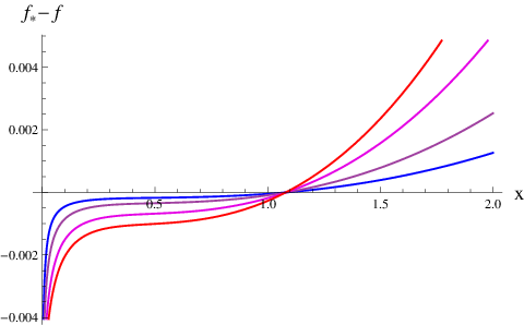
Upon expansion to linear order in , we recover the simplified expressions discussed before. The approach of Eq. (94) to the Gaußian fixed point written as the zeroth order result for the quasi-fixed-point condition, cf. Eq. (83), is shown in Fig. 20 for the case , and various values of the gauge coupling.
V.4 Linearized flow near the Gaußian fixed point
The standard way of characterizing the properties of the RG flow in the neighborhood of a fixed point is through linearization with respect to the displacement from the fixed point. Here we discuss how the analysis of such a linearized flow of the dimensionless potential relates to the construction of scaling solutions for . It should first be emphasized that while a fixed-point condition for differs from one for because of the supplementary boundary conditions, yielding different scaling phenomena, the information encoded in the differential equation, i.e. the flow equations, for and is one and the same. Hence, the UV asymptotics of the flows of the potential should be inside the flow equation for in vicinity of the Gaußian fixed point. Making the meaning of ’vicinity’ more precise requires a discussion of subtleties.
The analysis of the stability properties of the Gaußian fixed point can be reduced to an eigenvalue problem if one sets up an approximate description of the RG flow in terms of a linear operator. The standard construction proceeds by separating the RG-time dependence from the field-dependence [39]
| (95) | |||
| (96) |
i.e. considering and as -independent, and expanding the flow equations for and to linear order in . This provides an eigenvalue system for and , where the eigenvalue controls the RG evolution along the corresponding eigendirection, since . As , eigenvectors with must have and correspond to the usual purely-scalar Gaußian eigenperturbations with , . The case gives us the marginal interaction, which is marginally irrelevant in the standard analysis. The other marginal direction descends from keeping , and it corresponds to a scalar potential solving the marginality condition
| (97) |
implying up to field-independent constants
| (98) |
where is an integration constant. The other integration constant of this second order linear ODE needs to be set equal to zero otherwise the potential would have an exponential growth for large , which violates self-similarity of the linearized RG flow [39] (see the discussion in Sec. V.3.1). Here the only constraints on come from self-consistency of the linearized analysis, i.e. it should be sufficiently small, and from the stability of the corresponding potential, i.e. it should be positive. At the level of the eigenvalue analysis is also -independent by construction, on the same footing as and .
Beyond linearization, we already know that this perturbation cannot be exactly marginal. Indeed the eigenvalue problem simply illustrates the local properties of the RG flow. By consistency the solution given above should describe the leading asymptotics of the running scalar potential along the marginally relevant trajectory governed by the gauge coupling. Hence, we can replace the infinitesimal displacements from the fixed point and with their running counterparts and , and require that the corresponding potential vanishes when approaches zero. This is possible only if equals zero or if it is an appropriate function of . The first option is clearly not acceptable since it does not lead to stable potentials as in the analysis of [26], and furthermore it clashes with the freedom in the choice of allowed by the linearized analysis. On the other hand assuming to be a function of one can comply with all the requirements listed so far, as long as and .
Since we are still confining ourselves to the UV asymptotics, we can parametrize the small- behavior of this function by a simple power law , with and a sufficiently small . For the consistency of the linearized analysis yielding Eq. (98) for , we need to constrain ; otherwise would become of the same order of higher powers of that have been neglected in the linearization of the flow. Indeed, by translating the above formula for the linearized potential in terms of rescaled quantities and one obtains exactly the next-to-leading parametrizations of the -scaling solutions presented in Sec. V.3.1. The scaling solutions are beyond the scope of the present conventional linearized analysis, since one needs to consistently take into account higher powers of inside . Unfortunately, if one sticks to the variables and the next-to-leading power of appearing inside is and this comes together with nonlinearities and more explicit field-dependencies. This renders the function too complicated for an analytic functional treatment. However, if , its minimum and its derivatives scale like definite powers of , one does not need to take into account all of the -terms inside , and an intermediate approximation order becomes available between and . This is precisely what the rescaling in the definition of and accounts for.
V.5 Global analysis of the quasi-fixed-point potentials
An analysis of the flow for the full potential (or ) requires to consider the global properties of this partial differential equation in field space. So far, we have performed this analysis either in an effective-field-theory spirit (polynomial expansion in or ) or in terms of a weak-coupling expansion, each coming with its own limitations. In the following, we improve on both by considering the functional quasi-fixed-point condition at a given finite value of . As argued in general above and verified explicitly in various limits, the quasi-fixed-point condition describes a locus of points in theory space which gets closer and closer to the true asymptotically free trajectory for small gauge coupling. For increasing coupling, the solution to as a function of this coupling may still represent an acceptable approximation of the true RG trajectory. The technical advantage of solving the quasi-fixed-point condition clearly is that it corresponds to an ODE instead of the PDE of the full flow in and .
From the global viewpoint in field space, the expansions so far are not only expected to have a limited range of validity. By expanding the beta functional of in powers of or , we also modify the nonlinear structure of the flow equation, most importantly removing movable or fixed singularities. Indeed, these singularities of the flow equation are known to lead to rather selective criteria for the existence and physical eligibility of fixed-point solutions [38, 39, 78, 79, 43, 80, 81, 82, 83, 84]. Hence, the results obtained so far still have to pass the test of global existence and eligibility, as the expansions used so far might decisively change the behavior of for large fields or close to the origin. For a significant test, we need to maintain the singularity structure of the flow equations, and construct again quasi-fixed-point potentials .
For the following numerical analysis, we neglect the dependence of the anomalous dimensions on the expectation value of the scalar . This corresponds to dropping the scalar loops in the expressions of the anomalous dimensions and keeping only the gauge loops; (technically, this corresponds to setting or inside and ). For this is fully justified at weak coupling as the terms dropped are of higher order than the leading order . For , the expectation value is numerically small, also justifying the approximation. The latter also holds for except for non-generically small values of which we exclude from the following analysis. In summary, this approximation is quantitatively well justified, and, most importantly, does not significantly alter the functional structure of the flow equation. The remaining analysis of the solutions still requires numerical methods, since the quasi-fixed-point equation is of second order and highly nonlinear.
V.5.1 Shooting from the minimum
Let us start by numerically constructing the solution to the quasi-fixed-point equation for fixed values of first by shooting from the minimum. For a given value of , we expect the existence of a one parameter family of solutions labeled, for instance, by the parameter above. In fact, this problem at first sight seems very similar to that of constructing fixed point solutions for the scalar potential at Wilson-Fisher-type fixed points. We review the latter for completeness in App. B, where we demonstrate that the techniques used in the following can reproduce known results to a high accuracy. The quasi-fixed point condition can be rewritten into a conventional ODE form,
| (100) | |||||
where the numerator function depends nonlinearly on its arguments and can be straightforwardly computed from Eq. (77). Both, numerator and denominator function depend on . We integrate the ODE by starting from the minimum towards both smaller values (shooting inwards ) and larger values (shooting outwards ). The initial conditions,
| (101) |
a priori form a 2-parameter set of solutions. As in the well-known Wilson-Fisher case (App. B), the right-hand side of Eq. (100) has both a fixed singularity at , as well as a movable singularity at the point , where . Shooting outwards, the movable singularity is generically hit at some value , . The existence of a regular solution requires to fix one of the parameters, e.g., , such that also the numerator vanishes and the solution can go in a regular fashion through and be continued to .
In the Wilson-Fisher case, the fixed singularity at implying the condition also fixes the second parameter and thus only a discrete set of solutions exists, yielding a quantization of both physical fixed points as well as critical exponents. As discussed in App. B, this solution can be found by tuning the remaining parameter, say , to its critical value.
This is precisely the point, where the present nonabelian Higgs model in differs from the pure scalar case (in ): we have numerically not been able to satisfy the condition for curing the fixed singularity at for a wide range of numerically explored parameter regions . Whereas this seems like a reason for concern, it comes actually not unexpectedly, as the weak-coupling solutions studied above also partly exhibited singularities in the higher-derivatives of . In fact, we find that the potential and its first derivative stay numerically well-behaved down to rather small values of , see Fig. 26 . Very close to , the fixed singularity in eventually contaminates standard integration algorithms and the numerical integration stops. This behavior of a stable solution for and and a divergence in higher-derivatives is rather independent of the initial conditions at . Again, this is in contrast to the Wilson-Fisher case, where singularities in higher derivatives as well as the potential itself appear and depend strongly on initial conditions if the criterion is missed.
Still, singularities also in higher derivatives would represent a problem if they persisted in the limit , as this could contradict asymptotic freedom. In order to test this, we have determined the onset of the singularity near in the numerical solution as a function of . As a criterion, we have computed the position where , which is still in the region where and behave regularly and slowly varying, whereas the higher derivatives start to vary rapidly. An estimate of is shown in Fig. 21 for the case for a wide range of values. A fit to the data at small coupling confirms that the singular regime shrinks to zero for . Numerically, we find with for . A similar behavior is observed also for other values of .
In fact, for the description of this singular behavior close to seems within reach of the weak-coupling expansion, because the corresponding quasi-fixed-point potentials exhibit logarithmic structures, leading to divergences in their higher order derivatives. It is thus interesting to compare these features to those of the full numerical solution. Since the small field behavior is only weakly sensible to the position of the movable singularities at , we do not need to fine-tune the parameters to their quasi-fixed-point values as boundary conditions of the numerical integration. For definiteness, we insert values according to the leading weak-gauge-coupling quasi-fixed-point relation of Eq. (79). For instance, at we can use the approximation in Eq. (94), and relate as in the quasi-fixed-point case, even if is not tiny. The comparison between this analytic form and the numerical solution is shown in Fig. 22, where a discrepancy is visible in a neighborhood of the origin. This failure of the weak-coupling expansion is reasonable, since it relies on the assumption that the argument of the gauge-thresholds is big, which excludes values of much smaller than . Indeed, these plots show that this region progressively shrinks as decreases, such that the range of applicability of the analytic approximation gets larger.


We take these numerical studies as evidence that global solutions to the quasi-fixed-point equation exist. These solutions form a one-parameter family for each value of which can be parametrized, e.g., by the position of the minimum (alternatively, this could be rephrased in terms of a parameter as before). These solutions develop singularities in their higher derivatives near . This singular regime vanishes with such that the quasi-fixed-point potential approaches asymptotic freedom globally on field space.
As a further check, we can compare these numerical findings with the approximate results obtained in the effective-field-theory setting in the weak-coupling limit. If the numerical solutions obtained by shooting correspond to those of the effective-field-theory analysis, the minimum and the critical value for fixed by outward shooting should be tightly related for a given value of the gauge coupling . A comparison with the expansion of the potential in Eq. (29) implies to identify with the expansion coefficient of at the minimum, . From the effective-field-theory analysis, we hence expect in the weak-coupling limit
| (102) | |||||
| (103) | |||||
| (104) |
where Eq. (102) summarizes Eqs. (52) and (53), Eq. (103) follows from Eq. (42), and Eq. (104) arises from an analogous analysis of Eq. (38) if the next-to-leading order is included. The result of the comparison of our numerical studies with these analytical forms is shown in Fig. 23 as a function of for fixed for various values of . The analytical estimates Eqs. (103) and (104) are shown as dashed lines and agree with the full numerical curves for all the depicted values of and small values of . Interestingly, Eq. (103) also approximates the full numerical solution for for , while the proper analytic form Eq. (102) (dotted line) takes over for sufficiently small, (for , this asymptotics sets in for only much smaller values of and thus is not visible in this plot). We conclude that the numerical analysis of the full quasi-fixed-point equation agrees very well with the effective-field-theory analysis in the corresponding validity limit, lending support to the existence of asymptotically free trajectories in the nonabelian Higgs model.

V.5.2 Shooting from large fields
Another option to extract information from the quasi-fixed-point condition beyond the weak-field, weak-coupling expansion is to compute the large- asymptotic expansion of the quasi-fixed-point potential. This can be done for any and without neglecting subleading powers of ; in fact, no expansion in is involved in the following. The result is given in Eqs. (127) and (128). For the present discussion it suffices to refer to the leading term of this expansion, which is
| (105) | ||||
| (106) |
where is an arbitrary integration constant, while the subleading terms depend on , , , and itself. Since is always positive the scalar potential is stable as long as .
For the following analysis, we can again ignore the dependence of the anomalous dimensions. This is consistent with the large-field expansion, as the anomalous dimensions depend only on which is considered as much smaller than the expansion point , . Remarkably, in the approximation of neglecting the contribution of scalar loops to the anomalous dimensions, the latter are both negative and controlled by . This allows for the case which corresponds to and . Yet, already in the one-loop approximation such range of values is quite restricted, being . The contribution of the scalar loops to are positive and are expected to further restrict this bound. Quite in general, instead, AF requires to be a monotonically increasing function of , such that by choosing arbitrarily large we can make arbitrarily close to zero.
The analytic large-field asymptotic expansion (and its first derivative) can be used as a boundary condition at a large field value , for numerical integration of the quasi-fixed-point equation towards the origin [85]. This procedure can be called ‘shooting’, since it involves an arbitrary coefficient . The criterion for fixing this free parameter is usually provided by requirements on the behavior of the solutions at , which are absent in the present context. Hence, we expect to be able to construct a one-parameter family of solutions labeled by , which can then be related to the position of the nontrivial minimum or to the curvature . For consistency, one needs to make sure that the chosen is big enough, for instance, by checking that the values of , , are stable against an increase of . This procedure can be repeated for any , and must be adjusted correspondingly.
Such an analysis is important for testing the stability of the potential, for which a method capable of probing the large-field region is mandatory. For the weak coupling expansion is one such tool, since one can solve the ODE without requiring to be small. This is because the only nontrivial explicit -dependence of appears in the gauge loop, through the combination , such that small and large play the same role. For instead, the weak coupling expansion is not applicable when is kept fixed and is taken arbitrarily large. Also shooting from the minimum is not helpful, since the corresponding solution always hits a movable singularity for .
For definiteness, let us discuss in detail the case. The corresponding weak- expansion in Eq. (84) provides two crucial relationships: one between the large-field behavior of the potential () and the curvature at the minimum (), the other between this curvature and the position of the minimum. These are fulfilled also by the present numerical solutions to an accuracy controlled by the gauge coupling, see Figs. 24 and 25 respectively. In the limit, the deviations are roughly of the same order of magnitude as .


One can also compare the two solutions obtained by the two shooting procedures from a large field value or from the minimum . The two solutions have different ranges of applicability: while the former is accurate for the whole inner region , the latter is appropriate for , and quickly breaks down towards larger values of . Hence, we compare the two solutions in the domain of applicability of the latter. Since we provide different kinds of boundary conditions in the two cases, and since at non-tiny there is a small difference between and , we need to tune the parameters in such a way that the produced solutions have the same value of . These are compared to each other and to the analytic large-field asymptotics at a given value of in Fig. 26. This confirms the compatibility of the two approaches.

V.5.3 Large- approximation
The matrix can be diagonalized such that it reduces to . For SU() and pointing into the -direction in fundamental color space, one has
| (107) |
We have explicitly verified for various gauge groups that the spectrum does not depend on the direction of in the Cartan. The multiplicities in this spectrum scales with respectively, such that the first line in Eq. (107) seems to dominate in the large- limit. However, the combination that enters agrees with the the Casimir invariant and thus is in fact dominated by the second line of Eq. (107). In order to extract the large- limit of the flow equations, a rescaling is convenient
| (108) |
The flow equation in the limit then simplifies to
| (109) | |||||
| (110) | |||||
The dependence of on , together with the general expectation that holds because of the contribution of the gauge loops, makes the analysis of this system harder than a corresponding large- limit for purely scalar models or Yukawa models. To simplify the system, we use the observation that the finite values of exert a small quantitative influence on the flows in the weak coupling regime. As in the preceding analysis, we hence set in both anomalous dimensions and . As a consequence, these anomalous dimensions become simple functions of only. For instance, the one-loop expressions are re-obtained to lowest order (including the rescaling (108))
| (111) |
For instance, the full expression for in the limit consists of only the first line of Eq. (110), which most importantly contains the term in the one-loop beta-function of the quartic coupling (cf. Eq. (4)) as well as its RG improvement due to the presence of and inside . Let us introduce the notation
| (112) |
Then the flow equation for the potential function is a first order PDE which can be recast into the form of two inhomogeneous ODEs by the method of characteristics. By denoting , for the linear regulator these read
| (113) | |||||
| (114) |
where both and have to be interpreted as functions of only. The desired potential function is obtained from the previous system as the solution corresponding to the initial condition , representing the bare potential, and . Because of the difference between and at , the freedom to specify the function can be translated into a freedom in determining the running of the potential w.r.t. the RG time . This is another way of recognizing the freedom to choose a boundary condition for the integration of the RG equations. The goal of this subsection is to explicitly show how the latter allows for the construction of -scaling in the UV.
Unfortunately, this system of ODEs does not offer a straightforward explicit solution, though it could be solved numerically rather straightforwardly. For reasons of analytical insight, we perform another physically motivated simplification: the second term on the right-hand side of Eq. (114) arises from the would-be Goldstone modes. Owing to the Higgs mechanism, these modes are actually not propagating degrees of freedom, but remain visible here only because of our choice of using a Landau-type gauge. In particular, such contributions would be absent in unitary gauge which is more adapted to the physical degrees of freedom in the Higgs phase. Therefore, we drop these contributions in Eq. (114), which decouples the two solutions and makes the latter equation trivially solvable. It is interesting to note that this line of argument together with the large- limit removes the scalar-loop contributions to the flow of the scalar sector altogether. Hence, we expect the conventional triviality problem of perturbative nonabelian Higgs models to be alleviated in the current limit anyway.
In this limit, we can again go back to the PDE for the potential function , such that Eq. (109) reads
| (115) | |||||
Here and in the following, we use the lowest-order form Eq. (111) for the anomalous dimensions and ignore the dependence of the threshold function on . This makes Eq. (115) accessible to straightforward integration. The solution is a linear combination of the corresponding quasi-fixed-point solution and of the solution of the homogeneous flow equation. For the linear regulator in , it reads
| (116) | |||||
where is an arbitrary function that can depend on and only through its argument. From here, we can recover the -scaling solutions from different choices of . First, we go over from the variable to the gauge-rescaled field as used before, identifying ,
| (117) | |||||
We then look for finite limits of and when .
If the inhomogeneous solution corresponding to the second line becomes trivial in the limit (even though it this is not regular at ). In order to have a finite nontrivial potential then we need to demand for the homogeneous solution (first line) to remain different from zero. This is the case if when , such that when .
If it is sufficient to choose a function that approaches a constant for in order to recover the corresponding quasi-fixed-point solution; note that the different numerical factors in front of the inhomogeneous piece compared to the solutions arises from subleading terms of the expansion. We conclude that we rediscover the family of -scaling solutions towards asymptotic freedom also in the large- limit.
We observe that only the asymptotic behavior of for large argument is fixed by the requirement to realize asymptotic freedom in the UV. Apart from this asymptotic behavior, remains largely undetermined in the present approximation. Whereas this freedom does not affect the approach to asymptotic freedom, the shape of at finite argument can take influence on the IR behavior. For instance, if exhibited an exponential behavior for small argument,
| (118) |
this would correspond to a dimensionful relevant component, i.e., a nonvanishing dimensionful mass, which increases logarithmically with the gauge coupling towards the IR. Within the limitations of the current large- analysis, it is difficult to judge whether the freedom to choose (beyond the asymptotics which controls asymptotic freedom) is merely an artifact of the approximations or whether it can parametrize further relevant components as in Eq. (118).
VI IR flows and mass spectrum
Our analysis of the UV behavior of the model allowed us to classify the asymptotically free trajectories which are attracted by the Gaußian fixed point at high energies. In total, we found a four-parameter family of these trajectories which we label by . Whereas and are fixed parameters for each trajectory, the parameters and quantify the magnitude of the relevant component and the gauge coupling, respectively, at a reference scale . This reference scale is not physical, as a change of can be compensated by a corresponding change of and as dictated by the renormalization flow along the trajectory.
Once, the trajectory is chosen in terms of these parameters, the theory is fixed and all long-range observables can, in principle, be predicted. Technically, this corresponds to solving the full coupled PDE/ODE system of our truncation from down to the IR scales. For the initial conditions for this PDE/ODE system, we need to relate the parameters to the corresponding functions/variables. In particular, we have to fix the full potential at the initialization scale. We have argued that this can be approximated by the solution of a quasi-fixed-point equation. This approximation becomes better for smaller gauge coupling: the parametrizations obtained in the previous sections are trustworthy if the -dependent powers of appearing in Tab. 2 are small. Hence, this suggests to fix the initial conditions at scales much larger than any IR scale (e.g., the Fermi scale, or the scale where the gauge coupling grows large). Though using the quasi-fixed-point solution may introduce small errors in the irrelevant components as compared to the true scaling solution, RG universality guarantees that these errors are washed out by the RG flow towards IR scales. In practice, this suggests to compute the IR flow approximately in terms of a simple polynomial expansion of the potential. In fact, the reliability of such an expansion for a description of Fermi scale observables has been verified for a variety of standard-model-like (gauged)-Higgs-Yukawa models in [86, 87, 88, 89, 90].
However, there is an apparent clash: on the one hand, we can apply truncated polynomial (effective-field-theory-like) approximations for the IR flow of the potential; on the other hand, our asymptotically free UV scaling solutions require boundary conditions that fix higher-order couplings to gauge-rescaled dimensionless ratios and that give rise to a global existence of the potential in field space. For instance in the effective-field-theory setting, we have discovered the asymptotically free trajectories, provided that the ratios and
| (119) |
etc. approach nonvanishing constants in the UV. It is obvious that this property cannot meaningfully persist along the RG flow towards the IR: for instance, it would imply that the dimensionful couplings could diverge in the IR, e.g., the six-point vertex would scale as for , where is the -dependent power given in the second column of Tab. 1. This would correspond to a substantial deviation from Wilsonian power counting, being in strong contradiction to the anticipated vicinity of the Higgs sector to the Gaußian fixed point.
Therefore, we expect the scaling conditions such as Eq. (119) to be satisfied in the UV whereas Wilsonian scaling should hold in the IR. The quantitative details of the transition between the different scaling regimes are governed by the full PDE. In the present section, we aim at a simple estimate for the flow between the different regimes. For this purpose, we stay within the polynomial effective-field-theory setting and model the behavior of a higher-order coupling; it turns out that the results for the long-range observables only show a mild dependence on the details of this modeling.
It is worthwhile to compare the parameter fixing to that of conventional perturbation theory. In the latter case, the couplings would be fixed in terms of the long-range observables of Higgs mass , gauge boson mass and vacuum expectation value . These translate into renormalization conditions for, say , , and at a certain fixing scale . For the asymptotically free trajectories, we have one additional parameter. Say, we fix this additional one in terms of a concrete choice for . Next, we choose some (small) value of . The asymptotically free scaling potential can then be constructed from the quasi-fixed-point condition in conjunction with the choice for the third parameter . Now, in the simplest effective-field theory approximation including a term, we can trade for the ratio of Eq. (119) which approaches a constant in the deep UV. The choice of the four parameters is then completed by adding a value for the relevant direction. In practice, this value has a strong influence on the value of the Fermi scale, i.e., the value of the vacuum expectation value in units of . This choice of parameters fixes all initial conditions; e.g., in the effective-field-theory setting to order , also and are fixed by the quasi-fixed-point conditions at the scale in this manner.
Figure 27 shows a set of example flows for .


Here, we have chosen and naively kept fixed over all scales. The latter choice implies (fixing ), and the relevant component is varied such that is an integer number ranging from 1 to 9. Even for this unphysical case of keeping constant over all scales, we observe a freeze-out behavior of the dimensionful renormalized expectation value (upper panel) and quartic coupling (lower panel) towards the infrared at a scale for sufficiently big . This indicates the generation of the Fermi scale and the Higgs mass, and marks the decoupling of all massive modes. Only for much lower scales , the artificial choice of a constant spoils the decoupling behavior towards the deep IR, triggering an unphysical strong flow of and of . This signals the break down of the oversimplifying approximation of keeping constant on all scales, destabilizing the physical decoupling regime in the deep IR.
A simple approximation to model the UV to IR transition region is to switch from =const. to a fixed renormalized dimensionful coupling after the onset of the physical freeze-out behavior. A simple choice is even to set near decoupling, which is enough to achieve the freeze-out of . Resulting flows for the simplest choice with for are shown in Fig. 28 , again for and the same initial conditions as before.


The decoupling regime is now more stable (upper panel), facilitating to read off the physical long-range observables; for instance, the Higgs mass would correspond to . Only in the very deep IR, yet another pathological IR behavior sets in, which artificially drives (lower panel). This artifact is caused by the spurious presence of propagating would-be Goldstone bosons in the Landau gauge used here [87]. The dominating positive contribution of these modes to the scalar anomalous dimension drives the flow artificially in the very deep IR. This artifact would be absent in the unitary gauge.
The difference between the extreme choices of const. and for the flows is shown in Fig. 29 for the expectation value and the quartic coupling.


The quantitative difference in the physical decoupling regime is on the per mille level and decreases for a larger relevant component and a smaller initial . Of course, any smooth modeling of the transition regime from constant to vanishing is equally possible, but is expected to lead to even smaller differences.
In the examples shown in Figs. 27, 28, 29 the separation of scales between initialization and decoupling is rather small, as encoded in the ratio . Still, it is already visible that the details about the treatment of the nonrenormalizable interaction have a tiny effect on the IR spectrum, as long as the chosen boundary conditions allow to end up in a Higgs phase. This corroborates the expectation that boundary conditions compatible with asymptotic freedom in the UV and a Higgs phase in the IR can also preserve the IR-irrelevance of nonrenormalizable interactions. For phenomenological applications the separation of scales is expected to be larger, implying that the effect of different boundary conditions for nonrenormalizable operators will even be smaller.
Still, the task to compute phenomenologically viable flows is far from straightforward, as these would require the decoupling scale to be near the Fermi scale. At that scale, the gauge coupling should approach the physical value (as dictated by the boson mass relative to the vacuum expectation value), which is not small. As the quasi-fixed-point condition facilitates an accurate determination of the asymptotically free trajectory only for small gauge couplings, the flow of the trajectories has to be followed over many orders of magnitude, say from the Planck scale to the Fermi scale. In addition, the relevant component at the Planck scale has to be fine-tuned very accurately to trigger decoupling near the Fermi scale. This is a manifestation of the standard hierarchy problem in the present setting. Computing such a functional flow for a full potential over many orders of magnitude represents a viable challenge for modern FRG PDE solvers [91].
Here, we will follow a simpler pragmatic approach: we assume that RG flows from the asymptotically free trajectories, including suitable small relevant perturbations, ending up in the Higgs phase in the IR do exist. The preceding studies represent simple examples for such flows. In order to separate the UV regime from the Fermi scale, the parameter for the relevant direction has to be very small at a high UV scale . In fact, it has to have a negligible influence on a large part of the flow towards the IR until becomes sufficiently large at a cross-over (CO) scale where it kicks the system off the logarithmically slow running in the UV fixed point regime. In this way, the relevant direction triggers the approach to decoupling at . As the relevant perturbation increases with critical exponent , the cross-over scale will already be comparable to . At the cross-over scale, the four UV parameters can be mapped by the RG flow onto a set of four other suitable parameters, e.g., the values of the couplings in the effective-field-theory description . In principle, also the values of all higher order parameters are determined by the UV parameters; however, the full PDE would have to be solved accurately for a quantitative estimate. Nevertheless, as long as the flow ends up in the IR Higgs regime where Wilsonian power counting becomes applicable, the precise details do not matter but are washed out by the RG flow.
If so, this suggests to stay within the effective-field-theory viewpoint and set up the IR flow at a fiducial cross-over scale . Though it is difficult to relate the precise initial data at to the four UV parameters , we can at least estimate them by solving the quasi-fixed-point condition for the scalar sector with , and by superimposing a suitable relevant component with parameter . In other words, we model our ignorance about the effect of the relevant component on the relations among higher order couplings by suddenly and discontinuously switching on the relevant component at .
As a self-consistency check of this procedure, we can again study the sensitivity of the results in the decoupling regime to the details of how we treat the higher-order interactions, as we did before in the weak-coupling case. For this purpose, we now initialize the flow at the fiducial at a coupling value slightly below the desired and compute the flow towards decoupling in the const. as well as the approximation. All other parameters are chosen as before. Also for this bigger value of the initial gauge coupling, we observe that adding a relevant component is sufficient to drive the system towards decoupling in both approximations. The resulting differences for the field expectation value and the quartic coupling are shown in Fig. 30.


These differences are again found to be comparatively small though somewhat larger than before because of the larger gauge coupling. We conclude that different choices of boundary conditions for the running of , even those that would artificially violate its Wilsonian IR irrelevance such as for const., have only a minor effect on the properties at decoupling, even in the case that the initialization and decoupling scale are separated by less than one order of magnitude, and even for a larger value of the gauge coupling.
Within this simple effective-field-theory setting, we can now construct an approximate mapping of the four UV parameters onto the long range observables. As the gauge coupling is fixed by the desired IR value ( boson mass), and the relevant component is determined by ending up with a vacuum expectation value at the Fermi scale, GeV, a variation of the parameters and is expected to shift the Higgs mass.
In our approximate treatment, some care is required for the determination of the magnitude of the relevant component at the cross-over scale parametrized by . Self-consistency of our cross-over picture requires to be sufficiently small such that it is justified to ignore the relevant component at larger scales. On the other hand, should be sufficiently large such that it triggers to flow towards the decoupling regime. For instance, if would be chosen too small in our approximation, the physical decoupling could overlap with the artificial IR flow of the would-be Goldstone bosons which do not properly decouple in the Landau gauge in our approximation.
This gauge insufficiency also has the consequence that the decoupling is not visible in the gauge coupling, which is driven by gauge modes even in the deep IR in our approximation. This contaminates the freeze-out behavior of the flow of the mass and creates a minimum in as a function of instead of the plateau behavior which we observe for the Higgs mass and signals decoupling. If is chosen too large, the minimum in occurs at larger values than the plateau of , such that we cannot unambiguously identify the point of decoupling. This is shown in Fig. 31 for the case, where the running masses are exhibited for various choices for .
In summary, we observe that there is an interval of acceptable values of for any choice of and which is consistent with the physical and technical requirements listed above. This interval spans approximately an order of magnitude. Inside this interval we prefer small values of , as it simplifies the identification of the decoupling scale. For the sake of inspecting several and values at once, turns out to be a reasonable choice. By fixing this value to a constant, the physical Fermi scale in turn implicitly fixes the cross-over scale, such that only and remain as parameters.


With all these prerequisites, we are now ready to explore the properties of the mass spectrum. For this, we first estimate the initial data at the cross-over scale from the analytic parametrization of the asymptotically free trajectories obtained in Sec. V. Having fixed the Fermi scale as well as the boson mass by the choice of the gauge coupling at , we can then study the dependence of the Higgs mass on the parameters and . The ratio of Higgs to boson mass is shown in Fig. 32. We observe that each of the two parameters can be used to tune the Higgs mass. This is similar to perturbation theory where governs the Higgs mass. Hence, and are not uniquely fixed by the knowledge of the mass spectrum, since for each one can find a suitable . Indeed, these numerical scans show that the qualitative dependence of the mass ratio is well described by the same ratio at initialization, which in the cross-over picture is the same as the ratio at the fixed-point regime. We find
| (120) |
As a consequence, the theory is not fully specified by the mass spectrum and the Fermi scale contrary to the perturbative setting, but an additional higher-order operator has to be measured in order to determine the asymptotically free trajectory that can guarantee UV completion of the theory.

We close this section with the comment that the present estimate of IR observables is close to the spirit of a perturbative estimate of the spectrum. In particular, the present treatment is blind to nonperturbative bound-state effects triggered by the gauge sector. This becomes obvious from the fact that or could be chosen such that the system seemingly stays in the perturbatively massless phase. In fact, such a phase does not exist, as the gauge sector eventually grows strong towards the IR. As a consequence, the perturbatively massless phase actually corresponds to a QCD-like phase, with a massive spectrum of glueballs and corresponding gauge-Higgs bound states. The properties of and distinction between these phases has recently been under intense investigation [92, 93, 94]. A particular interesting question is as to whether the non-perturbative effects can exert a strong influence also on the Higgs side of the phase transition, e.g., in terms of providing a lower bound on the Higgs mass [94], or even reshape the spectrum in comparison with a pure perturbative reasoning [95, 96].
VII Conclusions
Our work demonstrates the construction of asymptotically free renormalization group trajectories in nonabelian Higgs models. We emphasize that we have identified these trajectories also for those models, where low-order perturbation theory does not exhibit asymptotic freedom. Whereas most of our analysis is performed at weak coupling, the essential difference to standard perturbation theory arises from the fact that we carefully pay attention to boundary conditions to be imposed on the renormalized action.
While perturbation theory is largely insensitive to boundary conditions and merely implicitly assumes that suitable boundary conditions exist, the importance of boundary conditions for the existence of scaling solutions is well known from the study of interacting fixed points in critical phenomena. Our work can be viewed as an extension of this concept to quasi-fixed points which solve a fixed-point condition for the scalar potential at finite but fixed gauge coupling. The corresponding scalar quasi-fixed-point potential yields an estimate of asymptotically free RG trajectories of the model becoming accurate in the limit of vanishing gauge coupling.
The set of asymptotically free models for a given gauge group SU() has four parameters which is one more than for a perturbative analysis. In the latter, nonabelian Higgs models have a relevant parameter (mass parameter of the scalar potential), the marginally relevant gauge coupling and the marginally irrelevant Higgs self-coupling. In our construction the relevant mass-like parameter persists and the marginally relevant gauge coupling goes along with a nontrivial perturbation of the scalar potential determined by the quasi-fixed-point conditions. The latter, however, can be solved in terms of two parameters for which we have not found any further constraint. They may be viewed as exactly marginal in an RG language.
While we have presented indications for this scenario first in the languages of simple low-order perturbation theory and effective field theory, the picture unfolds both more quantitatively and conceptually with the method of functional renormalization. This technique facilitates to extract global information about the scalar potential by means of analytic asymptotic expansions and numerical shooting methods. Most importantly, this function passes all standard tests of being polynomially (uniformly) bounded and self-similar for large field values. As an interesting feature which is different from pure scalar models for critical phenomena, we observe a logarithmic non-analyticity of the quasi-fixed-point potential at the origin in field space where the potential and its first derivative still stay finite. This non-analyticity implies that the asymptotically free trajectories globally belong to a different functional space than that spanned by polynomial interactions – even though many features of these trajectories are visible in polynomial effective-field-theory like approximations.
The formulation of the property of asymptotic freedom as a standard RG fixed-point condition allows to perform a standard Wilsonian RG relevance classification of perturbations about scaling solutions. In the weak-coupling regime, they exhibit a standard (quantized) behavior of the critical exponents. As a consequence, our asymptotically free trajectories may solve triviality problems but – within a perturbative analysis of the mass spectrum – they appear to feature the same properties with respect to a separation of hierarchies as the perturbative standard model.
The functional RG has also helped to further corroborate the evidence for such asymptotically free theories in the large- limit, where an even larger set of parameters in the form of a whole function seems admissible in order to find asymptotically free trajectories. While this might be an artifact of the large- limit, we have been able to rediscover unambiguously the family of trajectories parametrized by and , again corresponding to boundary conditions for the solution of the differential RG equations.
Whereas we have concentrated on pure nonabelian Higgs models, viewed as a key ingredient of the standard model or of suitable sectors of grand unified models, first signatures of the existence of the trajectories described here had already been found before in a gauged Yukawa model in [46]. That previous study had in fact been inspired by the search for asymptotically safe trajectories, potentially being triggered by a quasi-conformal running of the field expectation value [44, 45]. While the latter may still be a viable ingredient, our present results illustrate that such a property is not necessary for the construction of asymptotically free trajectories. As far as asymptotic safety is concerned, a wide class of gauged Higgs-Yukawa models has recently been identified that allows for a controlled determination of a non-trivial UV limit in terms of an interacting fixed point [97, 98, 99, 36, 100].
Finally, we have estimated the long-range properties of theories that arise from our asymptotically free trajectories, and identified initial/boundary conditions giving rise to a conventional Higgs phase. Whereas solving a full functional flow from a high UV scale down to the Fermi scale remains a technical challenge, our estimates give access to the particle spectrum analogous to perturbation theory. We observe that the range of particle masses remains unconstrained because of the freedom encoded in the parameters and . For a realistic application of such asymptotically free trajectories to standard model physics, the inclusion of chiral fermion degrees of freedom is, of course, mandatory.
Acknowledgements.
We thank Jörg Jäckel, Axel Maas, Christof Wetterich and Omar Zanusso for interesting discussions, and Stefan Rechenberger, René Sondenheimer, and Michael Scherer for collaboration on related projects. We acknowledge support by the DFG under grants No. GRK1523/2, and Gi 328/5-2 (Heisenberg program).Appendix A Lowest-order weak-coupling effective field theory
In the effective field theory analysis in Sect. III, we consider the functions fully in the spirit of effective field theory including all couplings of a given truncation as they would arise from corresponding Feynman diagrams. By contrast, the functional RG analysis in Sect. V is mostly based on a weak-coupling analysis, sorting the functions in powers of the gauge coupling and disregarding higher orders. This seems to imply a clash between the two approaches, as the functional RG analysis ignores terms that have been fully taken into account in the effective field theory analysis.
In this Appendix, we show that the lowest-order weak-coupling analysis can also be performed in the effective-field theory case. Though this is a rather crude approximation, results for the quasi-fixed-point values of the potential minimum and the rescaled coupling are maintained, and the error for the higher-order couplings is parametrically quantifiable. The order of the following results parallels that of the main text.
We start with the case discussed in Subsect. III.1. There the function in Eq. (III.1) contains terms of order and . Keeping both already suffices in order to unfold the gauge-rescaling pattern of the higher order terms. However, if we strictly impose a weak-coupling scheme, the leading-order analogue would simply read . Hence, is still a quasi-fixed point if . With being the all-order result, this lowest-order result implies an error of for the six-point coupling .
This observation generalizes to the generalized scaling solutions presented in Subsect. III.2: the function for to leading power in reads (cf. Eq. (27)),
| (121) |
Solving the quasi-fixed-point equation for at arbitrary , we find the simple solution . This simple leading-order estimate entails an error of in the determination of along the asymptotically free trajectory.
Let us now turn to the more general case that includes the relevant direction, i.e. a possibly nontrivial field expectation value. We start again with the case as discussed in Subsect. IV.1. To lowest order in the coupling, the functions for and read, cf. Eqs. (31) and (),
The quasi-fixed-point solution reproduces the correct value for , and suggests as before. Thus, the degree of accuracy of this approximation, as far as couplings beyond are concerned, would be the same as in the corresponding approximation without the relevant direction.
This pattern generalizes to as discussed in Subsect. IV.2: the lowest-order approximation does not affect in Eq. (38), so that the quasi-fixed point for remains correct at that order. The corresponding function for of Eq. (39) simplifies to with the solution , implying an error for of . The same pattern holds also for the lowest-order calculation for the case . The quasi-fixed-point values of Eq. (42) persist, whereas the result to lowest order would represent an error of order in the determination of along the asymptotically free trajectories.
For , the main text in Subsect. IV.4 and subsequent sections is already devoted to a leading-order analysis, yielding non-trivial values for at the quasi-fixed point. In conclusion, the effective-field theory and functional RG analysis are partly complementary, but fully agree with each other in the regime of overlapping applicability.
Appendix B Singularities, boundary conditions and free parameters of fixed point solutions
The determination and properties of fixed point solutions of functional RG equations is a widely studied subject. These so-called fixed functionals have been constructed for a wide variety of theories with different methods, see, e.g. [38, 39, 78, 101, 79, 43, 80, 81, 82, 83, 102, 84]. In the present work, we use the shooting method for an analysis of the solution space of the quasi-fixed-point potentials of the nonabelian Higgs model.
In order to highlight the similarities and differences to conventional models, let us start here with a short recap of the Wilson-Fisher fixed-point potential of the Ising model below . For the purpose of illustration, we use the simple local-potential approximation (LPA), ignoring anomalous dimensions, and use the piece-wise linear regulator. The fixed-point equation for the potential for the dimensionless order parameter then reads [76]
| (122) |
It is illustrative to write this ordinary differential equation as
| (123) |
and the numerator function being . Being a second order equation, the solution manifold is generally parametrized by two initial conditions. symmetry, requiring , reduces the solution manifold to only one parameter, e.g., the choice of . Still, there is no one-parameter family of fixed-point solutions, because of the fact that the scaling terms in the denominator of Eq. (123) generically exhibits a zero at some finite field amplitude when integrating the differential equation from to larger field values for a generic . This zero of indicates the presence of a movable singularity in the fixed point equation. This singularity can be lifted, if the numerator also vanishes sufficiently fast at the same field value, . This later condition effectively fixes (quantizes) the remaining parameter . For the Ising model, only one choice of yields a nontrivial fixed point potential which is globally defined for all ; this solution is stable, i.e., bounded from below and also matches the large-field asymptotics [38, 85].
As a second illustrative step, we rephrase the same model in the language of the invariant . The resulting flow equation for the potential can be obtained by rewriting Eq. (122) accordingly as well as from the flow equation (71) by dropping the gauge contributions and setting (as counts complex scalars). In the LPA, we can bring the fixed-point equation into the form similar to Eq. (123),
| (124) |
and the numerator function . In addition to the movable singularity arising from for some , there is now also a fixed singularity of the fixed point equation at . The latter even inhibits to naively integrate from to larger field values. Also, the boundary condition establishing symmetry is seemingly lost, as is already manifestly invariant.
In fact, invariance and the occurrence of the fixed singularity are connected: e.g., if a linear -violating term occurred in the potential near zero field, we would have and the derivatives exhibited singularities.
These issues of the formulation using the invariant field variable , can be resolved by constructing the fixed-point potential by starting from a finite field value. The two-dimensional manifold of solutions to Eq. (124) can, for instance, be parametrized by demanding for at a fiducial value for the minimum , and similarly for the curvature at the minimum. (Here we anticipated that the Wilson-Fisher fixed-point potential has a nonvanishing minimum. For other systems, alternative initial conditions can be chosen in terms of two parameters.) By starting from and integrating Eq. (124) both to larger and smaller field values, i.e., “shooting” outward and inward, we obtain a two-parameter family of solutions of Eq. (124). This time, the integrations yield global solutions, if both singularities are lifted by suitable conditions. As before, the movable singularity at has to be lifted by the condition . In addition, the fixed singularity at has to be lifted by the further condition . In total, we again obtain two conditions for the two-parameter family, which leads to a quantization of these parameters and a discrete set of fixed-point solutions. For , we have checked that this method rediscovers the Wilson-Fisher fixed-point potential, finding accurate agreement with the known literature values. E.g. the position of the minimum agrees on this accuracy level with the highest-precision data for the LPA obtained in [83].
Appendix C Asymptotic expansions for large field amplitudes
One remarkable property of functional RG equations like Eq. (77) is that they apply to arbitrarily large constant field amplitudes. The corresponding asymptotic properties of the potential often play a crucial role in constraining and characterizing the set of physically acceptable solutions. For the Higgs model such an equation has not only a functional dependence on the average field (as well as the location of the nontrivial minimum , which enters through the anomalous dimensions), but also a parametric dependence on the gauge coupling , and the interplay between these two quantities gives rise to a rich spectrum of possible behaviors.
In particular, we have been mainly concerned with the understanding of the set of consistent boundary conditions for quasi-fixed-point potentials. We have addressed the construction of these functional solutions, both in a weak coupling expansion and beyond. In the first case, the ODE defining the problem is provided by Eq. (80). For the case, we had to solve it numerically, and then the knowledge of the right large- behavior serves to validate/construct the corresponding solution. These quasi-fixed-point potentials must have an asymptotic behavior for large of the kind
| (125) |
where is an arbitrary integration constant, while all the rest is a function of and . We adopted an expansion up to , which is enough for the level of accuracy we are interested in. Retaining the full anomalous dimensions but neglecting terms of order , and denoting , one finds
| (126) | ||||
Since is positive and close to , the scalar potential is stable along such trajectories (the case is also stable but not bounded, just like the fixed point). Thus, it is not possible to split such a solution in a fixed-point potential plus a small fluctuation, since the latter would grow like for large field values.
As Eq. (80) arises by an expansion in , with respect to the full gauge dependence, this large-field asymptotics is valid in an intermediate field-amplitude regime, where is still sufficiently small. In other words, it applies in the double limit and , provided the latter is stronger than the former.
Clearly, to go beyond the weak gauge coupling approximation, we need a different asymptotic expansion. This can be obtained by directly analyzing the complete functional of Eq. (77), for any and . Furthermore, in computing this asymptotic expansion, it is convenient to keep and implicit. Hence, the result remains valid also upon retaining the full expressions (or even better approximations) for the anomalous dimensions. The first five terms of such an expansion turn out to be sufficient for our purposes,
| (127) | |||||
Again stays free, while the other parameters can be written as functions of , , , as follows:
| (128) | ||||
At this point one could ask whether the weak coupling approximation of this expression agrees with Eqs. (125) and (126) in the case. The agreement does occur at leading order, but it is restricted to the integer expansion terms in Eqs. (127) and (128). The reason for the discrepancy of the remaining terms lies in the fact the the two limits and do not commute, such that the two expansions refer to different asymptotic regions.
References
- [1] D. J. Gross and F. Wilczek, Phys. Rev. Lett. 30, 1343 (1973a).
- [2] H. D. Politzer, Phys. Rev. Lett. 30, 1346 (1973).
- [3] D. J. Gross and F. Wilczek, Phys. Rev. D8, 3633 (1973b).
- [4] D. J. Gross and F. Wilczek, Phys. Rev. D9, 980 (1974).
- [5] H. D. Politzer, Phys. Rept. 14, 129 (1974).
- [6] T. P. Cheng, E. Eichten, and L.-F. Li, Phys. Rev. D9, 2259 (1974).
- [7] F. A. Bais and H. A. Weldon, Phys. Rev. D18, 1199 (1978).
- [8] D. J. E. Callaway, Phys. Rept. 167, 241 (1988).
- [9] K. G. Wilson and J. B. Kogut, Phys. Rept. 12, 75 (1974).
- [10] J. Frohlich, Nucl. Phys. B200, 281 (1982).
- [11] M. Luscher and P. Weisz, Nucl. Phys. B290, 25 (1987).
- [12] M. Luscher and P. Weisz, Nucl. Phys. B295, 65 (1988).
- [13] M. Luscher and P. Weisz, Nucl. Phys. B318, 705 (1989).
- [14] A. Hasenfratz, K. Jansen, C. B. Lang, T. Neuhaus, and H. Yoneyama, Phys. Lett. B199, 531 (1987).
- [15] U. M. Heller, H. Neuberger, and P. M. Vranas, Nucl. Phys. B399, 271 (1993), arXiv:hep-lat/9207024 [hep-lat] .
- [16] U. Wolff, Phys. Rev. D79, 105002 (2009), arXiv:0902.3100 [hep-lat] .
- [17] P. V. Buividovich, Nucl. Phys. B853, 688 (2011), arXiv:1104.3459 [hep-lat] .
- [18] O. J. Rosten, JHEP 07, 019 (2009), arXiv:0808.0082 [hep-th] .
- [19] M. Gockeler, R. Horsley, V. Linke, P. E. L. Rakow, G. Schierholz, and H. Stuben, Phys. Rev. Lett. 80, 4119 (1998), arXiv:hep-th/9712244 [hep-th] .
- [20] H. Gies and J. Jaeckel, Phys. Rev. Lett. 93, 110405 (2004), arXiv:hep-ph/0405183 [hep-ph] .
- [21] L. D. Landau, in Niels Bohr and the Development of Physics, ed. Wolfgang Pauli, London: Pergamon Press.
- [22] M. Gell-Mann and F. E. Low, Phys. Rev. 95, 1300 (1954).
- [23] N.-P. Chang, Phys. Rev. D10, 2706 (1974).
- [24] N.-P. Chang and J. Perez-Mercader, Phys. Rev. D18, 4721 (1978), [Erratum: Phys. Rev.D19,2515(1979)].
- [25] E. S. Fradkin and O. K. Kalashnikov, J. Phys. A8, 1814 (1975).
- [26] A. Salam and J. A. Strathdee, Phys. Rev. D18, 4713 (1978).
- [27] A. Salam and V. Elias, Phys. Rev. D22, 1469 (1980).
- [28] G. F. Giudice, G. Isidori, A. Salvio, and A. Strumia, JHEP 02, 137 (2015), arXiv:1412.2769 [hep-ph] .
- [29] B. Holdom, J. Ren, and C. Zhang, JHEP 03, 028 (2015), arXiv:1412.5540 [hep-ph] .
- [30] W. Zimmermann, Commun. Math. Phys. 97, 211 (1985).
- [31] R. Oehme and W. Zimmermann, Commun. Math. Phys. 97, 569 (1985).
- [32] S. Heinemeyer, J. Kubo, M. Mondragon, O. Piguet, K. Sibold, W. Zimmermann, and G. Zoupanos, (2014), arXiv:1411.7155 [hep-ph] .
- [33] J. Hetzel and B. Stech, Phys. Rev. D91, 055026 (2015), arXiv:1502.00919 [hep-ph] .
- [34] G. M. Pelaggi, A. Strumia, and S. Vignali, JHEP 08, 130 (2015), arXiv:1507.06848 [hep-ph] .
- [35] C. Pica, T. A. Ryttov, and F. Sannino, (2016), arXiv:1605.04712 [hep-th] .
- [36] E. Molgaard and F. Sannino, (2016), arXiv:1610.03130 [hep-ph] .
- [37] H. Gies and L. Zambelli, Phys. Rev. D92, 025016 (2015), arXiv:1502.05907 [hep-ph] .
- [38] A. Hasenfratz and P. Hasenfratz, Nucl. Phys. B270, 687 (1986).
- [39] T. R. Morris, Nonperturbative QCD: Structure of the QCD vacuum, Prog. Theor. Phys. Suppl. 131, 395 (1998), arXiv:hep-th/9802039 [hep-th] .
- [40] T. R. Morris, Nucl. Phys. B495, 477 (1997), arXiv:hep-th/9612117 [hep-th] .
- [41] T. R. Morris and M. D. Turner, Nucl. Phys. B509, 637 (1998), arXiv:hep-th/9704202 [hep-th] .
- [42] J. A. Dietz and T. R. Morris, JHEP 01, 108 (2013), arXiv:1211.0955 [hep-th] .
- [43] M. Demmel, F. Saueressig, and O. Zanusso, JHEP 08, 113 (2015), arXiv:1504.07656 [hep-th] .
- [44] H. Gies and M. M. Scherer, Eur. Phys. J. C66, 387 (2010), arXiv:0901.2459 [hep-th] .
- [45] H. Gies, S. Rechenberger, and M. M. Scherer, Eur. Phys. J. C66, 403 (2010), arXiv:0907.0327 [hep-th] .
- [46] H. Gies, S. Rechenberger, M. M. Scherer, and L. Zambelli, Eur. Phys. J. C73, 2652 (2013), arXiv:1306.6508 [hep-th] .
- [47] S. Browne, L. O’Raifeartaigh, and T. Sherry, Nucl. Phys. B99, 150 (1975).
- [48] V. Kaplunovsky, Nucl. Phys. B211, 297 (1983).
- [49] B. W. Lee and W. I. Weisberger, Phys. Rev. D10, 2530 (1974).
- [50] S. R. Coleman and E. J. Weinberg, Phys. Rev. D7, 1888 (1973).
- [51] L. Fei, S. Giombi, and I. R. Klebanov, Phys. Rev. D90, 025018 (2014), arXiv:1404.1094 [hep-th] .
- [52] L. Fei, S. Giombi, I. R. Klebanov, and G. Tarnopolsky, Phys. Rev. D91, 045011 (2015), arXiv:1411.1099 [hep-th] .
- [53] R. Percacci and G. P. Vacca, Phys. Rev. D90, 107702 (2014), arXiv:1405.6622 [hep-th] .
- [54] I. F. Herbut and L. Janssen, Phys. Rev. D93, 085005 (2016), arXiv:1510.05691 [hep-th] .
- [55] P. Mati, (2016), arXiv:1601.00450 [hep-th] .
- [56] A. Eichhorn, L. Janssen, and M. M. Scherer, (2016), arXiv:1604.03561 [hep-th] .
- [57] I. H. Bridle and T. R. Morris, (2016), arXiv:1605.06075 [hep-th] .
- [58] O. J. Rosten, Phys. Rept. 511, 177 (2012), arXiv:1003.1366 [hep-th] .
- [59] K. Halpern and K. Huang, Phys. Rev. Lett. 74, 3526 (1995), arXiv:hep-th/9406199 [hep-th] .
- [60] K. Halpern and K. Huang, Phys. Rev. D53, 3252 (1996a), arXiv:hep-th/9510240 [hep-th] .
- [61] V. Periwal, Mod. Phys. Lett. A11, 2915 (1996), arXiv:hep-th/9512108 [hep-th] .
- [62] A. Bonanno, Phys. Rev. D62, 027701 (2000), arXiv:hep-th/0001060 [hep-th] .
- [63] H. Gies, Phys. Rev. D63, 065011 (2001), arXiv:hep-th/0009041 [hep-th] .
- [64] T. R. Morris, Phys. Rev. Lett. 77, 1658 (1996), arXiv:hep-th/9601128 [hep-th] .
- [65] K. Halpern and K. Huang, Phys. Rev. Lett. 77, 1659 (1996b).
- [66] C. Wetterich, Phys. Lett. B301, 90 (1993).
- [67] K. Aoki, Methods of renormalization group. Proceedings, Summer School on mathematical physics, Tokyo, Japan, September 23-26, 1999, Int. J. Mod. Phys. B14, 1249 (2000).
- [68] J. Berges, N. Tetradis, and C. Wetterich, Phys. Rept. 363, 223 (2002), arXiv:hep-ph/0005122 [hep-ph] .
- [69] J. M. Pawlowski, Annals Phys. 322, 2831 (2007), arXiv:hep-th/0512261 [hep-th] .
- [70] H. Gies, ECT* School on Renormalization Group and Effective Field Theory Approaches to Many-Body Systems Trento, Italy, February 27-March 10, 2006, Lect. Notes Phys. 852, 287 (2012), arXiv:hep-ph/0611146 [hep-ph] .
- [71] B. Delamotte, Lect. Notes Phys. 852, 49 (2012), arXiv:cond-mat/0702365 [cond-mat.stat-mech] .
- [72] J. Braun, J. Phys. G39, 033001 (2012), arXiv:1108.4449 [hep-ph] .
- [73] U. Ellwanger, M. Hirsch, and A. Weber, Z. Phys. C69, 687 (1996), arXiv:hep-th/9506019 [hep-th] .
- [74] D. F. Litim and J. M. Pawlowski, Phys.Lett. B435, 181 (1998), arXiv:hep-th/9802064 [hep-th] .
- [75] L. F. Abbott, Nucl. Phys. B185, 189 (1981).
- [76] D. F. Litim, Phys. Lett. B486, 92 (2000), arXiv:hep-th/0005245 [hep-th] .
- [77] D. F. Litim, Phys. Rev. D64, 105007 (2001), arXiv:hep-th/0103195 [hep-th] .
- [78] C. Bervillier, B. Boisseau, and H. Giacomini, Nucl. Phys. B789, 525 (2008), arXiv:0706.0990 [hep-th] .
- [79] A. Codello and G. D’Odorico, Phys. Rev. Lett. 110, 141601 (2013), arXiv:1210.4037 [hep-th] .
- [80] J. A. Dietz and T. R. Morris, JHEP 04, 118 (2015), arXiv:1502.07396 [hep-th] .
- [81] G. P. Vacca and L. Zambelli, Phys. Rev. D91, 125003 (2015), arXiv:1503.09136 [hep-th] .
- [82] T. Hellwig, A. Wipf, and O. Zanusso, (2015), arXiv:1508.02547 [hep-th] .
- [83] J. Borchardt and B. Knorr, Phys. Rev. D91, 105011 (2015), arXiv:1502.07511 [hep-th] .
- [84] D. F. Litim and E. Marchais, (2016), arXiv:1607.02030 [hep-th] .
- [85] T. R. Morris, Phys. Lett. B334, 355 (1994), arXiv:hep-th/9405190 [hep-th] .
- [86] H. Gies, C. Gneiting, and R. Sondenheimer, Phys. Rev. D89, 045012 (2014), arXiv:1308.5075 [hep-ph] .
- [87] H. Gies and R. Sondenheimer, Eur. Phys. J. C75, 68 (2015), arXiv:1407.8124 [hep-ph] .
- [88] A. Eichhorn, H. Gies, J. Jaeckel, T. Plehn, M. M. Scherer, and R. Sondenheimer, JHEP 04, 022 (2015), arXiv:1501.02812 [hep-ph] .
- [89] J. Borchardt, H. Gies, and R. Sondenheimer, (2016), arXiv:1603.05861 [hep-ph] .
- [90] A. Jakovac, I. Kaposvari, and A. Patkos, (2015), arXiv:1508.06774 [hep-th] .
- [91] J. Borchardt and B. Knorr, Phys. Rev. D94, 025027 (2016), arXiv:1603.06726 [hep-th] .
- [92] A. Maas, Mod. Phys. Lett. A28, 1350103 (2013), arXiv:1205.6625 [hep-lat] .
- [93] A. Maas and T. Mufti, JHEP 04, 006 (2014), arXiv:1312.4873 [hep-lat] .
- [94] A. Maas and T. Mufti, Phys. Rev. D91, 113011 (2015), arXiv:1412.6440 [hep-lat] .
- [95] A. Maas, Mod. Phys. Lett. A30, 1550135 (2015), arXiv:1502.02421 [hep-ph] .
- [96] A. Maas and P. Törek, (2016), arXiv:1607.05860 [hep-lat] .
- [97] D. F. Litim and F. Sannino, JHEP 12, 178 (2014), arXiv:1406.2337 [hep-th] .
- [98] A. D. Bond and D. F. Litim, (2016), arXiv:1608.00519 [hep-th] .
- [99] A. Codello, K. Langæble, D. F. Litim, and F. Sannino, JHEP 07, 118 (2016), arXiv:1603.03462 [hep-th] .
- [100] B. Bajc and F. Sannino, (2016), arXiv:1610.09681 [hep-th] .
- [101] J. Braun, H. Gies, and D. D. Scherer, Phys. Rev. D83, 085012 (2011), arXiv:1011.1456 [hep-th] .
- [102] N. Ohta, R. Percacci, and G. P. Vacca, Phys. Rev. D92, 061501 (2015), arXiv:1507.00968 [hep-th] .