Efficient Solution of Parameter Dependent Quasiseparable Systems and Computation of Meromorphic Matrix Functions

P. Boito Affiliation: XLIM–MATHIS, UMR 7252 CNRS Université de Limoges, 123 avenue Albert Thomas, 87060 Limoges Cedex, France. Email: paola.boito@unilim.fr Affiliation: CNRS, Université de Lyon, Laboratoire LIP (CNRS, ENS Lyon, Inria, UCBL), 46 allée d’Italie, 69364 Lyon Cedex 07, France. Y. Eidelman Affiliation: School of Mathematical Sciences, Raymond and Beverly Sackler Faculty of Exact Sciences, Tel-Aviv University, Ramat-Aviv, 69978, Israel. Email: eideyu@post.tau.ac.il L. Gemignani Affiliation: Dipartimento di Informatica, Università di Pisa, Largo Bruno Pontecorvo, 3 - 56127 Pisa, Italy. Email: l.gemignani@di.unipi.it

Abstract

In this paper we focus on the solution of shifted quasiseparable systems and of more general parameter dependent matrix equations with quasiseparable representations. We propose an efficient algorithm exploiting the invariance of the quasiseparable structure under diagonal shifting and inversion. This algorithm is applied to compute various functions of matrices. Numerical experiments show that this approach is fast and numerically robust.

Keywords: Quasiseparable matrices , shifted linear system, QR factorization, matrix function, matrix equation.

2010 MSC: 65F15

1 Introduction

In this paper we propose a novel method for computing the solution of shifted quasiseparable systems and of more general parameter dependent linear matrix equations with quasiseparable representations. We show that our approach has also a noticeable potential for effectively solving some large-scale algebraic problems that reduce to evaluating the action of a quasiseparable matrix function to a vector.

Quasiseparable matrices, characterized by the property that off-diagonal blocks have low rank, have found their application in several branches of applied mathematics and engineering. In the last decade there has been major interest in developing fast algorithms for working with such matrices [6, 7, 20, 19]. The quasiseparable structure arises in the discretization of continuous operators, as a consequence of the local properties of the discretization schemes, and/or because of the decaying properties of the operator or its finite approximations.

It is a celebrated fact that operations with quasiseparable matrices can be performed in linear time with respect to their size. In particular, the QR factorization algorithm presented in [5] computes in linear time a QR decomposition of a quasiseparable matrix $A\in\mathbb{C}^{N\times N}$ . This decomposition takes the special form $A=V\cdot U\cdot R$ , where $R$ is upper triangular, whereas $U$ and $V$ are banded unitary matrices. It turns out that the matrix $V$ only depends on the generators of the strictly lower triangular part of $A$ . This implies that any shifted linear system $A+\sigma I_{N}$ , $\sigma\in\mathbb{C}$ , can also be factored as $A+\sigma I_{N}=V\cdot U_{\sigma}\cdot R_{\sigma}$ for suitable $U_{\sigma}$ and $R_{\sigma}$ .

Relying upon this fact, in this paper we design an efficient algorithm for solving a sequence of shifted quasiseparable linear systems. The invariance of the factor $V$ can be exploited to halve the overall computational cost. Section 2 illustrates the potential of our approach using motivating examples and applications. In Section 3 we describe the novel algorithm by proving its correctness. Finally, in Section 4 we present several numerical experiments where our method is applied to the computation of $f(A)v$ and to the solution of linear matrix equations. The results turn out to be as accurate as classical approaches and timings are consistent with the improved complexity estimates.

2 Motivating Examples

In this section we describe two motivating examples from applied fields that lead to the solution of several shifted or parameter dependent quasiseparable linear systems.

2.1 A Model Problem for Boundary Value ODEs

Consider the non-local boundary value problem in a linear finite dimensional normed space $X=\mathbb{R}^{N}$ :

\frac{d{\mbox{\boldmath$v$}}}{dt}=A\mbox{\boldmath$v$},\quad 0<t<\tau,

(2.1)

\frac{1}{\tau}\int_{0}^{\tau}\mbox{\boldmath$v$}(t)\;dt=\mbox{\boldmath$g$}

(2.2)

where $A$ is a linear operator in $\mathbb{R}^{N}$ and $\mbox{\boldmath$g$}\in\mathbb{R}^{N}$ is a given vector.

The nonlocal problem of the form (2.1), (2.2) has been a subject of intensive study, see the papers by I. V. Tikhonov [18, 17], as well as [8] and the literature cited therein.

Under the assumption that all the numbers $\mu_{k}=2\pi ik/\tau,\;k=\pm 1,\pm 2,\pm 3,\dots$ are regular points of the operator $A$ the problem (2.1), (2.2) has a unique solution. Moreover this solution is given by the formula

\mbox{\boldmath$v$}(t)=q_{t}(A)\mbox{\boldmath$g$},\quad q_{t}(z)=\frac{\tau ze^{zt}}{e^{z\tau}-1}.

(2.3)

Without loss of generality one can assume that $\tau=2\pi$ .

Expanding the function $q_{t}(z)$ in the Fourier series of $t$ we obtain

q_{t}(z)=1+\sum_{k\in{\mathbb{Z}}/\{0\}}\frac{ze^{ikt}}{z-ik},\quad 0<t<2\pi.

We consider the equivalent representation with the real series given by

q_{t}(z)=1+2\sum_{k=1}^{\infty}z(z\cos kt-k\sin kt)(z^{2}+k^{2})^{-1},\quad 0<t<2\pi.

Using the formula

-\frac{k}{z^{2}+k^{2}}=\frac{z^{2}}{k(k^{2}+z^{2})}-\frac{1}{k}

we find that

q_{t}(z)=1+2\sum_{k=1}^{\infty}z(z\cos kt+\frac{1}{k}z^{2}\sin kt)(z^{2}+k^{2})^{-1}-2z\sum_{k=1}^{\infty}\frac{1}{k}\sin kt,\quad 0<t<2\pi

and since

2\sum_{k=1}^{\infty}\frac{1}{k}\sin kt=\pi-t,\quad 0<t<2\pi

we arrive at the following formula

q_{t}(z)=1+2\sum_{k=1}^{\infty}(z\cos kt+\frac{1}{k}z^{2}\sin kt)(z^{2}+k^{2})^{-1}-z(\pi-t),\quad 0<t<2\pi.

Thus we obtain the sought expansion of the solution $\mbox{\boldmath$v$}(t)$ of the problem (2.1), (2.2):

v(t)=g-(\pi-t)Ag+2\sum_{k=1}^{\infty}(A\cos kt+\frac{1}{k}A^{2}\sin kt)(A^{2}+k^{2}I_{N})^{-1}Ag,\quad 0\leq t\leq 2\pi.

(2.4)

Under the assumptions

\|(A-ikI_{N})^{-1}\|\leq\frac{C}{|k|},\quad k=\pm 1,\pm 2,\dots

(2.5)

and by using the Abel transform one can check that the series in (2.4) converges uniformly in $t\in[0,2\pi]$ . Hence, by continuity we extend here the formula (2.4) for the solution on all the segment $[0,2\pi]$ . The rate of convergence of the series in (2.4) is the same as for the series $\sum_{k=1}^{\infty}\frac{1}{k^{2}}$ . The last may be improved using standard techniques for series acceleration but by including higher degrees of $A$ . Indeed set

C_{k}(t)=A\cos kt+\frac{1}{k}A^{2}\sin kt.

Using the identity

(A^{2}+k^{2}I)^{-1}=\frac{1}{k^{2}}I-\frac{1}{k^{2}}A^{2}(A^{2}+k^{2}I)^{-1}

we get

\sum_{k=1}^{\infty}C_{k}(t)(A^{2}+k^{2}I_{N})^{-1}Ag=\sum_{k=1}^{\infty}\frac{1}{k^{2}}C_{k}(t)Ag-\sum_{k=1}^{\infty}\frac{1}{k^{2}}C_{k}(t)(A^{2}+k^{2}I)^{-1}A^{3}g.

The first entry here has the form

\sum_{k=1}^{\infty}\frac{1}{k^{2}}C_{k}(t)Ag=\sum_{k=1}^{\infty}\left(\frac{\cos kt}{k^{2}}A^{2}g+\frac{\sin kt}{k^{3}}A^{3}g\right).

Using the formulas

\sum_{k=1}^{\infty}\frac{\cos kt}{k^{2}}=\frac{\pi^{2}}{6}-\frac{\pi}{2}t+\frac{t^{2}}{4},\quad\sum_{k=1}^{\infty}\frac{\sin kt}{k^{3}}=\frac{\pi^{2}}{6}t-\frac{\pi}{4}t^{2}+\frac{t^{3}}{12},

we get

v(t)=V_{0}(t)g+V_{1}(t)Ag+V_{2}(t)A^{2}g+V_{3}(t)A^{3}g-2\sum_{k=1}^{\infty}\frac{1}{k^{2}}C_{k}(t)(A^{2}+k^{2}I)^{-1}A^{3}g.

(2.6)

with

V_{0}(t)=1,\;V_{1}(t)=t-\pi,\;V_{2}(t)=\frac{\pi^{2}}{3}-{\pi}t+\frac{t^{2}}{2},\;V_{3}(t)=\frac{\pi^{2}}{3}t-\frac{\pi}{2}t^{2}+\frac{t^{3}}{6}.

Summing up, our proposal consists in approximating the solution $\mbox{\boldmath$v$}(t)$ of the problem (2.1), (2.2) by the finite sum

v_{\ell}(t)=g-(\pi-t)Ag+2\sum_{k=1}^{\ell}(A\cos kt+\frac{1}{k}A^{2}\sin kt)(A^{2}+k^{2}I_{N})^{-1}Ag,\quad 0\leq t\leq 2\pi,

(2.7)

or using (2.6) by the sum

	$\displaystyle\hat{v}_{\ell}(t)=\sum_{j=0}^{3}V_{j}(t)A^{j}g$
	$\displaystyle-2\sum_{k=1}^{\ell}\frac{1}{k^{2}}(A\cos kt+\frac{1}{k}A^{2}\sin kt)(A^{2}+k^{2}I_{N})^{-1}A^{3}g,\quad 0\leq t\leq 2\pi,$		(2.8)

where $\ell$ is suitably chosen by checking the convergence of the expansion.

The computation of $\mbox{\boldmath$v$}_{\ell}(t_{i})\simeq\mbox{\boldmath$v$}(t_{i})$ , $0\leq i\leq M+1$ , requires the solution of a possibly large set of the shifted systems of the form

(A+\sigma_{i}I_{N})\mbox{\boldmath$x$}_{i}=\mbox{\boldmath$y$},\quad i=1,\dots,\ell.

(2.9)

The same conclusion applies to the problem of computing the function of a quasiseparable matrix whenever the function can be represented as a series of partial fractions. The classes of meromorphic functions admitting such a representation were investigated for instance in [14]. Other partial fraction approximations of certain analytic functions can be found in [12]. In the next section we describe an effective algorithm for this task.

As additional context for this model problem, note that a numerical approximation of the solution can be obtained by using the discretization of the boundary value problem on a grid and the subsequent application of the cyclic reduction approach discussed in [1]. This approach can be combined with techniques for preserving an approximate quasiseparable structure in recursive LU-based solvers: see the recent papers [2, 4, 10]. The approximate quasiseparable structure of functions of quasiseparable matrices has also been investigated in [13].

2.2 Sylvester-type Matrix Equations

As a natural extension of the problem (2.9), the right-hand side $y$ could also depend on the parameter $\sigma$ , that is, $\mbox{\boldmath$y$}=\mbox{\boldmath$y$}(\sigma)$ and $\mbox{\boldmath$y$}_{i}=\mbox{\boldmath$y$}(\sigma_{i})$ , $i=1,\dots,\ell$ . This situation is common in many applications such as control theory, structural dynamics and time-dependent PDEs [11]. In this case, the systems to be solved take the form

AX+XD=Y,\quad A\in\mathbb{R}^{N\times N},\ D=\mbox{\rm{diag}}\left[\sigma_{1},\ldots,\sigma_{\ell}\right],\ Y=\left[\mbox{\boldmath$y$}_{1},\ldots,\mbox{\boldmath$y$}_{\ell}\right].

Using the Kronecker product this matrix equation can be rewritten as a bigger linear system $\mathcal{A}\,\mbox{\rm{vec}}(X)=\mbox{\rm{vec}}(Y)$ , where $\mathcal{A}=I_{\ell}\otimes A+D^{T}\otimes I_{N}\in\mathbb{R}^{N\ell\times N\ell}$ , $\mbox{\rm{vec}}(X)=\left[\mbox{\boldmath$x$}_{1}^{T},\ldots,\mbox{\boldmath$x$}_{\ell}^{T}\right]^{T}$ , $\mbox{\rm{vec}}(Y)=\left[\mbox{\boldmath$y$}_{1}^{T},\ldots,\mbox{\boldmath$y$}_{\ell}^{T}\right]^{T}$ .

The extension to the case where $D$ is replaced by a lower triangular matrix $L=(l_{i,j})\in\mathbb{R}^{\ell\times\ell}$ is based on the backward substitution technique which amounts to solve

(A+l_{i,i}I_{N})\mbox{\boldmath$x$}_{i}=\mbox{\boldmath$y$}_{i}-\sum_{j=i+1}^{\ell}l_{i,j}\mbox{\boldmath$x$}_{j},\quad i=\ell\colon-1\colon 1.

(2.10)

Such approach has been used in different related contexts where the considered Sylvester equation is occasionally called a sparse-dense equation [16]. The classical reduction proposed by Bartels and Stewart [3] makes it possible to deal with a general matrix $F$ by first computing its Schur decomposition $F=ULU^{H}$ and then solving $A(XU)+(XU)L=YU$ . The resulting approach is well suited especially when the size of $A$ is large w.r.t. the number of shifts. If $A$ is quasiseparable then (2.10) again reduces to computing a sequence of shifted systems having the same structure in the lower triangular part and the method presented in the next section can be used.

3 The basic algorithm

Let us first recall the definition of quasiseparable matrix structure and quasiseparable generators. See [6] for more details.

Definition 3.1.

A block matrix $A=(A_{i,j})_{i,j=1}^{N}$ , with block entries $A_{i,j}\in\mathbb{R}^{m_{i}\times m_{j}}$ , is said to have lower quasiseparable generators $P(i)\in\mathbb{R}^{m_{i}\times r^{L}_{i-1}}\ (i=2,\dots,N)$ , $Q(j)\in\mathbb{R}^{r^{L}_{j}\times m_{j}}\ (j=1,\dots,N-1)$ , $\Xi(k)\in\mathbb{R}^{r^{L}_{k}\times r^{L}_{k-1}}\ (k=2,\dots,N-1)$ of orders $r^{L}_{k}\;(k=1,\dots,N-1)$ and upper quasiseparable generators $G(i)\in\mathbb{R}^{m_{i}\times r^{U}_{i}}(i=1,\dots,N-1)$ , $H(j)\in\mathbb{R}^{r^{U}_{j-1}\times m_{j}}\ (j=2,\dots,N)$ , $\Theta(k)\in\mathbb{R}^{r^{U}_{k-1}\times r^{U}_{k}}\,(k=2,\dots,N-1)$ of orders $r^{U}_{k}\;(k=1,\dots,N-1)$ if

A_{i,j}=\left\{\begin{array}[]{ll}P(i)\Xi_{i,j}^{>}Q(j)\ {\rm if}\ 1\leq j<i\leq N,\\ G(i)\Theta_{i,j}^{<}H(j)\ {\rm if}\ 1\leq i<j\leq N,\end{array}\right.

where $\Xi_{i,j}^{>}=\Xi(i-1)\cdots\Xi(j+1)$ for $i>j+1$ and $\Xi_{j+1,j}=I_{r^{L}_{j}}$ , and, similarly, $\Theta_{i,j}^{<}=\Theta(i+1)\cdots\Theta(j-1)$ for $j>i+1$ and $\Theta_{i,i+1}=I_{r^{U}_{i}}$ .

If $A$ admits such a representation, is is said to be $(r_{L},r_{U})$ -quasiseparable. Diagonal entries are stored separately, that is, we set $\Lambda(i)=A_{i,i}\in\mathbb{R}^{m_{i}\times m_{i}}$ .

The same representation can be applied to complex matrices.

We have denoted the quasiseparable generators by capital letters, as it is often done for matrices. Note however that the generators can be numbers, vectors or matrices, depending on the quasiseparable orders $r_{L_{i}},r_{U_{j}}$ and on the block sizes $m_{i},m_{j}$ .

To solve the systems (2.9), (2.10) we rely upon the QR factorization algorithm described in [5] (see also Chapter 20 of [6]). At first we compute the factorization

A+\sigma I=V\cdot T_{\sigma}

(3.11)

with a unitary matrix $V$ and a lower banded, or a block upper triangular, matrix $T_{\sigma}$ . It turns out that the matrix $V$ does not depend on $\sigma$ at all and moreover an essential part of the quasiseparable generators of the matrix $T_{\sigma}$ do not depend on $\sigma$ either. So a relevant part of the computations for all the values of $\sigma$ only needs to be performed once. Thus the problem is reduced to the solution of the set of the systems

T_{\sigma}\mbox{\boldmath$x$}_{\sigma}=V^{H}\mbox{\boldmath$y$}_{i},\quad\sigma=\sigma_{i},\;i=1,\dots,\ell.

(3.12)

The inversion of every matrix $T_{\sigma}$ as well as the solution of the corresponding linear system is significantly simpler than for the original matrix. We compute the factorization

T_{\sigma}=U_{\sigma}R_{\sigma}

(3.13)

with a block upper triangular unitary matrix $U_{\sigma}$ and upper triangular $R_{\sigma}$ and solve the systems

R_{\sigma}\mbox{\boldmath$x$}_{\sigma}=U_{\sigma}^{H}V^{H}\mbox{\boldmath$y$}_{i}.

(3.14)

Thus we obtain our main algorithm, which takes as input a set of quasiseparable generators for $A$ , shifts $\sigma_{i}$ and right-hand block vectors $\mbox{\boldmath$y$}_{i}$ , and outputs the solutions $\mbox{\boldmath$x$}_{i}$ of the linear systems $(A+\sigma_{i}I)\mbox{\boldmath$x$}_{i}=\mbox{\boldmath$y$}_{i}$ . The algorithm is comprised of two parts.

•

Part 1 computes useful quantities that are common to all the linear systems, namely, quasiseparable generators for $V$ in the factorization (3.11), and some quasiseparable generators for each $T_{\sigma_{i}}$ that do not actually depend on $\sigma_{i}$ .
•

Part 2 uses the results of Part 1, along with input data, to solve efficiently each linear system (which is why it begins with a loop over all the systems). For each $i=1,\ldots,\ell$ it computes the factorization (3.13), and then solves the triangular system (3.14).

Note that each of the matrices $V$ and $U_{\sigma_{i}}$ can also be factored as the product of $N$ “small” unitary matrices, which are denoted as $V_{k}$ and $U_{k}^{(i)}$ , respectively, in the algorithm that follows. Throughout the algorithm, these factored representations are computed via successive QR factorizations of suitable matrices and then used to compute products by $V^{H}$ or $U_{\sigma_{i}}^{H}$ in $O(N)$ time: see the proof of the algorithm for more details.

The sentences in italics explain the purpose of each block of instructions.

Main algorithm

Input:

•
quasiseparable generators for the block matrix $A$ , with entries $(A_{i,j})_{i,j=1}^{N}$ of sizes $m_{i}\times m_{j}$ , namely:
- –
  
  lower quasiseparable generators $P(i)\;(i=2,\dots,N),\;Q(j)\;(j=1,\dots,N-1),\;\Xi(k)\;(k=2,\dots,N-1)$ of orders $r^{L}_{k}\;(k=1,\dots,N-1)$ ,
- –
  
  upper quasiseparable generators $G(i)\;(i=1,\dots,N-1),\;H(j)\;(j=2,\dots,N),\;\Theta(k)\;(k=2,\dots,N-1)$ of orders $r^{U}_{k}\;(k=1,\dots,N-1)$ ,
- –
  
  diagonal entries $\Lambda(k)\;(k=1,\dots,N)$ ;
•

complex numbers $\sigma_{i},\;i=1,\dots,\ell$ ;
•

block vectors $\mbox{\boldmath$y$}_{i}=(y_{i}(k))_{k=1}^{N}$ with $m_{k}$ - dimensional coordinates $y(k)$ .

Output: solutions $\mbox{\boldmath$x$}^{(i)}=\mbox{\boldmath$x$}_{\sigma_{i}},\;i=1,\dots,\ell$ of the systems (3.12).

Part 1.

1.

Initialize auxiliary quantities:

$\rho_{N}=0,\quad\rho_{k-1}=\min\{m_{k}+\rho_{k},\;r^{L}_{k-1}\},\quad k=N,\dots,2,\;\rho_{0}=0,$

$\rho^{\prime}_{k}=\rho_{k}+r^{U}_{k},\;k=1,\dots,N-1,\quad\nu_{k}=m_{k}+\rho_{k}-\rho_{k-1},\;k=1,\dots,N.$

Compute the quasiseparable representation of the matrix $V$ (that is, generators with subscript _V) and the basic elements of the representation of the matrix $T_{\sigma}$ (that is, generators with subscript _T), as well as the vector $\mbox{\boldmath$w$}_{i}=V^{H}\mbox{\boldmath$y$}_{i}$ . Note that this is done through the computation of the “small” unitary factors $V_{k}$ of $V$ .

–

Using the QR factorization or another algorithm compute the factorization

$P(N)=V_{N}\left(\begin{array}[]{c}X_{N}\\ 0_{\nu_{N}\times r^{L}_{N-1}}\end{array}\right),$ (3.15)

where $V_{N}$ is a unitary matrix of sizes $m_{N}\times m_{N}$ , $X_{N}$ is a matrix of sizes $\rho_{N-1}\times r^{L}_{N-1}$ .

Determine the matrices $P_{V}(N),\Lambda_{V}(N)$ of sizes $m_{N}\times\rho_{N-1},m_{N}\times\nu_{N}$ from the partition

$V_{N}=\left(\begin{array}[]{cc}P_{V}(N)&\Lambda_{V}(N)\end{array}\right).$ (3.16)

Compute

$\left(\begin{array}[]{c}H_{T}(N)\\ \Lambda_{T}(N)\end{array}\right)=\left(\begin{array}[]{c}H(N)\\ V_{N}^{H}\Lambda(N)\end{array}\right),$ (3.17)

$\left(\begin{array}[]{c}c_{N,i}\\ w_{i}(N)\end{array}\right)=V^{H}_{N}y_{i}(N),\quad 1\leq i\leq\ell$ (3.18)

with the matrices $H_{T}(N),\Lambda_{T}(N),c_{N,i},w_{i}(N)$ of sizes $\rho^{\prime}_{N-1}\times m_{N},\nu_{N}\times m_{N},\rho_{N-1}\times 1,\nu_{N}\times 1$ respectively.

Set

$\Gamma_{N}=\left(\begin{array}[]{c}0_{r^{U}_{N-1}\times m_{N}}\\ P_{V}^{H}(N)\end{array}\right).$ (3.19)

–

For $k=N-1,\dots,2$ perform the following.

Using the QR factorization or another algorithm compute the factorization

\left(\begin{array}[]{c}P(k)\\ X_{k+1}\Xi(k)\end{array}\right)=V_{k}\left(\begin{array}[]{c}X_{k}\\ 0_{\nu_{k}\times r^{L}_{k-1}}\end{array}\right),

(3.20)

where $V_{k}$ is a unitary matrix of sizes $(m_{k}+\rho_{k})\times(m_{k}+\rho_{k})$ , $X_{k}$ is a matrix of sizes $\rho_{k-1}\times r^{L}_{k-1}$ .

Determine the matrices $P_{V}(k),Q_{V}(k),\Xi_{V}(k),\Lambda_{V}(k)$ of sizes $m_{k}\times\rho_{k-1},\rho_{k}\times\nu_{k},\rho_{k}\times\rho_{k-1}$ , $m_{k}\times\nu_{k}$ from the partition

V_{k}=\left(\begin{array}[]{cc}P_{V}(k)&\Lambda_{V}(k)\\ \Xi_{V}(k)&Q_{V}(k)\end{array}\right).

(3.21)

Compute

\left(\begin{array}[]{cc}H_{T}(k)&\Theta_{T}(k)\\ \Lambda_{T}(k)&G_{T}(k)\end{array}\right)=\left(\begin{array}[]{cc}I_{r^{U}_{k-1}}&0\\ 0&V_{k}^{H}\end{array}\right)\left(\begin{array}[]{ccc}H(k)&\Theta(k)&0\\ \Lambda(k)&G(k)&0\\ X_{k+1}Q(k)&0&I_{\rho_{k}}\end{array}\right).

(3.22)

with the matrices $H_{T}(k),\Theta_{T}(k),\Lambda_{T}(k),G_{T}(k)$ of sizes $\rho^{\prime}_{k-1}\times m_{k},\rho^{\prime}_{k-1}\times\rho^{\prime}_{k},\nu_{k}\times m_{k},\nu_{k}\times\rho^{\prime}_{k}$ respectively.

Set

\Gamma_{k}=\left(\begin{array}[]{c}0_{r^{U}_{k-1}\times m_{k}}\\ P_{V}^{H}(k)\end{array}\right)

(3.23)

and compute

\left(\begin{array}[]{c}c_{k,i}\\ w_{i}(k)\end{array}\right)=V_{k}^{H}\left(\begin{array}[]{c}y_{i}(k)\\ c_{k+1,i}\end{array}\right),\quad 1\leq i\leq\ell

(3.24)

with the vector columns $c_{k,i},w_{i}(k)$ of sizes $\rho_{k-1},\nu_{k}$ respectively.

–

Set $V_{1}=I_{\nu_{1}}$ and

\Lambda_{T}(1)=\left(\begin{array}[]{c}\Lambda(1)\\ X_{2}Q(1)\end{array}\right),\;G_{T}(1)=\left(\begin{array}[]{cc}G(1)&0\\ 0&I_{\rho_{1}}\end{array}\right),\quad\Gamma_{1}=\left(\begin{array}[]{c}I_{m_{1}}\\ 0_{\rho_{1}\times m_{1}}\end{array}\right),

(3.25)

w_{i}(1)=V_{1}^{H}\left(\begin{array}[]{c}y_{i}(1)\\ c_{2,i}\end{array}\right),\quad 1\leq i\leq\ell.

(3.26)

Part 2.

For $i=1,\dots,\ell$ (that is, for each shifted linear system) perform the following:

Compute the factorization $T_{\sigma_{i}}=U_{\sigma_{i}}R_{\sigma_{i}}$ and the vector $\mbox{\boldmath$v$}^{(i)}=\mbox{\boldmath$v$}_{\sigma_{i}}=U_{\sigma_{i}}^{H}\mbox{\boldmath$w$}_{i}$ , $\mbox{\boldmath$w$}_{i}=V^{H}\mbox{\boldmath$y$}_{i}$ . In particular, compute the “small” unitary factors $U_{k}^{(i)}$ of $U_{\sigma_{i}}$ and use this factorization to determine the quasiseparable generators of $T_{\sigma_{i}}$ , denoted by the subscript _T, and the vector $\mbox{\boldmath$v$}^{(i)}$ .

–

Compute the QR factorization

\Lambda_{T}(1)+\sigma_{i}\Gamma_{1}=U_{1}^{(i)}\left(\begin{array}[]{c}\Lambda_{R}^{(i)}(1)\\ 0_{\rho_{1}\times m_{1}}\end{array}\right),

(3.27)

where $U_{1}^{(i)}$ is a $\nu_{1}\times\nu_{1}$ unitary matrix and $\Lambda_{R}^{(i)}(1)$ is an upper triangular $m_{1}\times m_{1}$ matrix.

Compute

\left(\begin{array}[]{c}G_{R}^{(i)}(1)\\ Y_{1}^{(i)}\end{array}\right)=(U_{1}^{(i)})^{H}G_{T}(1),

(3.28)

\left(\begin{array}[]{c}v^{(i)}(1)\\ {\alpha}^{(i)}_{1}\end{array}\right)=(U_{1}^{(i)})^{H}w_{i}(1)

(3.29)

with the matrices $G_{R}^{(i)}(1),v^{(i)}(1),Y_{1}^{(i)},{\alpha}^{(i)}_{1}$ of sizes $m_{1}\times\rho^{\prime}_{1},m_{1}\times 1,\rho_{1}\times\rho^{\prime}_{1},\rho_{1}\times 1$ .

–

For $k=2,\dots,N-1$ perform the following.

Compute the QR factorization

\left(\begin{array}[]{c}Y^{(i)}_{k-1}(H_{T}(k)+\sigma_{i}\Gamma_{k})\\ \Lambda_{T}(k)+\sigma_{i}\Lambda_{V}^{H}(k)\end{array}\right)=U_{k}^{(i)}\left(\begin{array}[]{c}\Lambda_{R}^{(i)}(k)\\ 0_{\rho_{k}\times m_{k}}\end{array}\right),

(3.30)

where $U_{k}^{(i)}$ is an $(m_{k}+\rho_{k})\times(m_{k}+\rho_{k})$ unitary matrix and $\Lambda_{R}^{(i)}(k)$ is an $m_{k}\times m_{k}$ upper triangular matrix.

Compute

\left(\begin{array}[]{c}G_{R}^{(i)}(k)\\ Y_{k}^{(i)}\end{array}\right)=(U_{k}^{(i)})^{H}\left(\begin{array}[]{c}Y^{(i)}_{k-1}\Theta_{T}(k)\\ G_{T}(k)\end{array}\right),

(3.31)

\left(\begin{array}[]{c}v^{(i)}(k)\\ {\alpha}^{(i)}_{k}\end{array}\right)=(U_{k}^{(i)})^{H}\left(\begin{array}[]{c}{\alpha}^{(i)}_{k-1}\\ w_{i}(k)\end{array}\right)

(3.32)

with the matrices $G_{R}^{(i)}(k),v^{(i)}(k),Y_{k}^{(i)},{\alpha}^{(i)}_{k}$ of sizes $m_{k}\times\rho^{\prime}_{k},m_{k}\times 1,\rho_{k}\times\rho^{\prime}_{k},\rho_{k}\times 1$ .

–

Compute the $QR$ factorization

\left(\begin{array}[]{c}Y^{(i)}_{N}H_{T}(N)+\sigma_{i}\Gamma_{N}\\ \Lambda_{T}(N)+\sigma_{i}\Lambda_{V}^{H}(N)\end{array}\right)=U^{(i)}_{N}\Lambda_{R}^{(i)}(N),

(3.33)

where $U^{(i)}_{N}$ is a unitary matrix of sizes $(\nu_{N}+\rho_{N-1})\times(\nu_{N}+\rho_{N-1})$ and $\Lambda_{R}^{(i)}(N)$ is an upper triangular matrix of sizes $m_{N}\times m_{N}$ .

Compute

v^{(i)}(N)=(U^{(i)}_{N})^{H}\left(\begin{array}[]{c}{\alpha}^{(i)}_{N-1}\\ w_{i}(N)\end{array}\right).

(3.34)

4.
Solve the system $R_{\sigma_{i}}\mbox{\boldmath$x$}^{(i)}=\mbox{\boldmath$v$}^{(i)}$ , using the previously computed quasiseparable generators.
- –
  
  Compute
  
  $x^{(i)}(N)=(\Lambda_{R}^{(i)}(N))^{-1}v^{(i)}(N),$
  
  $\eta^{(i)}_{N-1}=(H_{T}(N)+\sigma_{i}\Gamma_{N})v^{(i)}(N)$
- –
  
  For $k=N-1,\dots,2$ compute
  
  $x^{(i)}(k)=(\Lambda_{R}^{(i)}(k))^{-1}(v^{(i)}(k)-G_{R}^{(i)}(k)\eta^{(i)}_{k}),$
  
  $\eta^{(i)}_{k-1}=\Theta_{T}(k)\eta^{(i)}_{k}+(H_{T}(k)+\sigma_{i}\Gamma_{k})x^{(i)}(k).$
- –
  
  Compute
  
  $x^{(i)}(1)=(\Lambda_{R}^{(i)}(1))^{-1}(v^{(i)}(1)-G_{R}^{(i)}(1)\eta^{(i)}_{1})$

Proof of correctness. The shifted matrix $A+\sigma I_{N}$ has the same lower and upper quasiseparable generators as the matrix $A$ and diagonal entries $\Lambda(k)+\sigma I_{m_{k}}\;(k=1,\dots,N)$ . To compute the factorization (3.11) we apply Theorem 20.5 from [6], obtaining the representation of the unitary matrix $V$ in the form

V=\tilde{V}_{N}\tilde{V}_{N-1}\cdots\tilde{V}_{2}\tilde{V}_{1},

(3.35)

where

\tilde{V}_{1}=V_{1}\oplus I_{\phi_{1}},\quad\tilde{V}_{k}=I_{\eta_{k}}\oplus V_{k}\oplus I_{\phi_{k}},\;k=2,\dots,N-1,\quad\tilde{V}_{N}=I_{\eta_{N}}\oplus V_{N}

with $\eta_{k}=\sum_{j=1}^{k-1}m_{j},\;\phi_{k}=\sum_{j=k+1}^{N}m_{j}$ and $(m_{k}+\rho_{k})\times(m_{k}+\rho_{k})$ unitary matrices $V_{k}$ , as well as the formulas (3.15), (3.16), (3.20), (3.21), $V_{1}=I_{\nu_{1}}$ . Here we see that the matrix $V$ does not depend on $\sigma$ . Moreover the representation (3.35) yields the formulas (3.18), (3.24), (3.26) to compute the vectors $\mbox{\boldmath$w$}_{i}=V^{H}\mbox{\boldmath$y$}_{i}$ , $1\leq i\leq\ell$ .

Next we apply the corresponding formulas from the same theorem to compute diagonal entries $\Lambda_{T}^{\sigma}(k)\;(k=1,\dots,N)$ and upper quasiseparable generators $G_{T}^{\sigma}(i)\;(i=1,\dots,N-1),\;H_{T}^{\sigma}(j)\;(j=2,\dots,N),\;\Theta_{T}^{\sigma}(k)\;(k=2,\dots,N-1)$ of the matrix $T_{\sigma}$ . Hence, we obtain that

	$\displaystyle\left(\begin{array}[]{c}H_{T}^{\sigma}(N)\\ \Lambda_{T}^{\sigma}(N)\end{array}\right)=\left(\begin{array}[]{cc}I_{r^{U}_{N-1}}&0\\ 0&V_{N}^{H}\end{array}\right)\left(\begin{array}[]{c}H(N)\\ \Lambda(N)+\sigma I_{m_{N}}\end{array}\right),$
	$\displaystyle\left(\begin{array}[]{cc}\Lambda_{T}^{\sigma}(1)&G_{T}^{\sigma}(1)\end{array}\right)=\left(\begin{array}[]{ccc}\Lambda(1)+\sigma I_{m_{1}}&G(1)&0\\ X_{2}Q(1)&0&I_{\rho_{1}}\end{array}\right),$

and for $k=N-1,\ldots,2$ ,

\left(\begin{array}[]{cc}H_{T}^{\sigma}(k)&\Theta_{T}^{\sigma}(k)\\ \Lambda_{T}^{\sigma}(k)&G_{T}^{\sigma}(k)\end{array}\right)=\left(\begin{array}[]{cc}I_{r^{U}_{k-1}}&0\\ 0&V_{k}^{H}\end{array}\right)\left(\begin{array}[]{ccc}H(k)&\Theta(k)&0\\ \Lambda(k)+\sigma I_{m_{k}}&G(k)&0\\ X_{k+1}Q(k)&0&I_{\rho_{k}}\end{array}\right).

From here we obtain the formulas

\begin{gathered}H_{T}^{\sigma}(k)=H_{T}(k)+\sigma\Gamma_{k},\;k=N,\dots,2,\\ \Lambda_{T}^{\sigma}(k)=\Lambda_{T}(k)+\sigma\Lambda_{V}^{*}(k),\;k=N,\dots,2,\quad\Lambda_{T}^{\sigma}(1)=\Lambda_{T}(1)+\sigma\Gamma_{1},\\ G_{T}^{\sigma}(k)=G_{T}(k),\;k=1,\dots,N-1,\quad\Theta_{T}^{\sigma}(k)=\Theta_{T}(k),\;k=2,\dots,N-1\end{gathered}

(3.36)

with $H_{T}(k),\Lambda_{T}(k),G_{T}(k),\Theta_{T}(k)$ and $\Gamma_{k}$ as in (3.17), (3.19), (3.22), (3.23) and (3.25).

Now by applying Theorem 20.7 from [6] to the matrices $T_{\sigma_{i}},\;i=1,2,\dots,M$ with the generators determined in (3.36) we obtain the formulas (3.27), (3.28), (3.30), (3.31), (3.33) to compute unitary matrices $U_{k}^{(i)}$ and quasiseparable generators of the upper triangular $R_{\sigma_{i}}$ such that $T_{\sigma_{i}}=U_{\sigma_{i}}R_{\sigma_{i}}$ , where

U_{\sigma_{i}}=\tilde{U}_{1}^{(i)}\tilde{U}_{2}^{(i)}\cdots\tilde{U}_{N-1}^{(i)}\tilde{U}_{N}^{(i)}

(3.37)

with

\tilde{U}^{(i)}_{1}=U^{(i)}_{1}\oplus I_{\phi_{1}},\quad\tilde{U}^{(i)}_{k}=I_{\eta_{k}}\oplus U^{(i)}_{k}\oplus I_{\phi_{k}},\;k=2,\dots,N-1,\quad\tilde{U}^{(i)}_{N}=I_{\eta_{N}}\oplus U^{(i)}_{N}.

Moreover the representation (3.37) yields the formulas (3.29), (3.32), (3.34) to compute the vector $\mbox{\boldmath$v$}^{(i)}=U^{H}_{\sigma_{i}}\mbox{\boldmath$w$}_{i}$ , $1\leq i\leq l$ .

Finally applying Theorem 13.13 from [6] we obtain Step 2.2 to compute the solutions of the systems $R_{\sigma_{i}}\mbox{\boldmath$x$}^{(i)}=\mbox{\boldmath$v$}_{(i)}$ . $\hfill\Box$

Concerning the complexity of the previous algorithm we observe that, under the simplified assumptions of $r^{L}_{k}=r^{U}_{k}=r$ , $m_{i}=m_{j}=m$ and $r\ll m$ , the cost of step 1 is of the order $(6r^{2}m+2m^{2})(Nm)$ , whereas the cost of step 2 can be estimated as $(2m^{2}\ell)(Nm)$ arithmetic operations. Therefore, the proposed algorithm saves at least half of the overall cost of solving $\ell$ shifted quasiseparable linear systems.

4 Numerical Experiments

The proposed fast algorithm has been implemented in MATLAB.¹¹ 1 The code is available at http://www.unilim.fr/pages_perso/paola.boito/software.html. All the experiments were performed on a MacBookPro equipped with MATLAB R2016b.

Example 4.1.

Let us test the computation of functions of quasiseparable matrices via series expansion, as outlined in Section 2. We choose $A$ as the $100\times 100$ one-dimensional discretized Laplacian with zero boundary conditions, which is $(1,1)$ -quasiseparable, and $g$ as a random vector with entries taken from a uniform distribution over $[0,1]$ . Define

v_{ex}=2\pi Ae^{At}(e^{2\pi A}-I)^{-1}g,

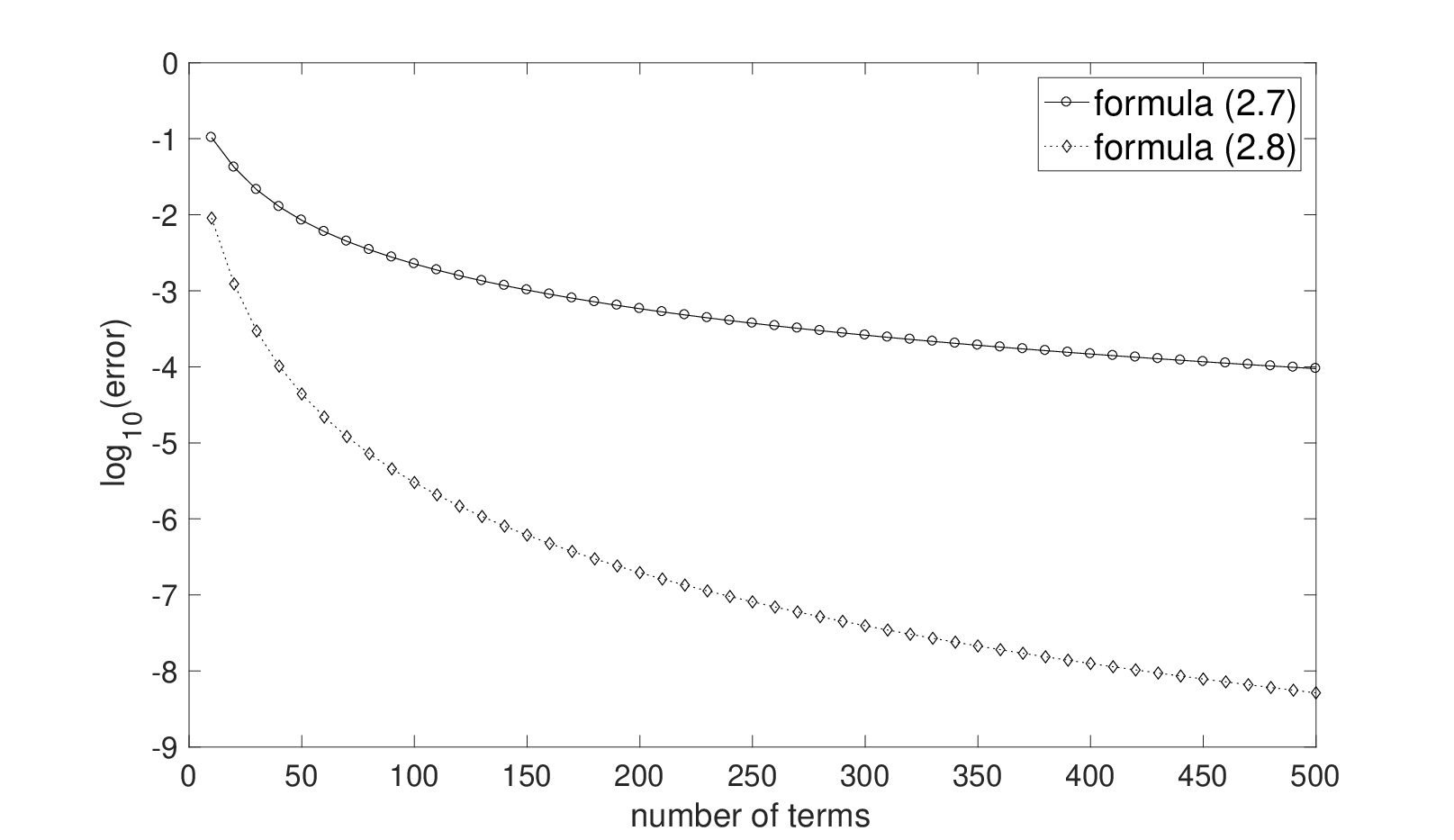
as exact solution (computed in multiprecision) to the problem (2.1), (2.2). Let $v_{\ell}$ and $\hat{v}_{\ell}$ be the approximate solutions obtained from (2.7) and (2.8), respectively, with $\ell$ expansion terms. Figures 1 and 2 show logarithmic plots of the absolute normwise errors $\|v_{ex}-v_{\ell}\|_{2}$ and $\|v_{ex}-\hat{v}_{\ell}\|_{2}$ for $t=\pi/2$ and $t=\pi/12$ , and values of $\ell$ ranging from $10$ to $500$ . The results clearly confirm that the formulation (2.8) has improved convergence properties with respect to (2.7). Note that the decreasing behavior of the errors is not always monotone.

It should be pointed out that, in this approach, a faster convergence of the series expansion gives a faster method for approximating the solution vector with a given accuracy. Indeed, the main computational effort comes from the solution of the shifted linear systems $(A^{2}+k^{2}I_{N})\mbox{\boldmath$x$}_{k}=Ag$ or $(A^{2}+k^{2}I_{N})\mbox{\boldmath$x$}_{k}=A^{3}g$ , and it is therefore proportional to the number of terms in the truncated expansion.

Refer to caption — Figure 1: Results for Example 4.1 for $t=\pi/2$ . This is a logarithmic plot of the errors given by the application of formulas (2.7) (circles with solid line) and (2.8) (diamonds with dotted line) for the computation of a matrix function times a vector.

Example 4.2.

This example is taken from [15], Example 3.3. We consider here the matrix $A\in\mathbb{R}^{2500\times 2500}$ stemming from the centered finite difference discretization of the differential operator $-\Delta u+10u_{x}$ on the unit square with homogeneous Dirichlet boundary condition. Note that $A$ has (scalar) quasiseparability order $50$ , but it can also be seen as block $1$ -quasiseparable with block size $50$ .

We want to compute the matrix function

A^{\frac{1}{2}}b\approx\sum_{k=1}^{\ell}\kappa_{k}(\omega_{k}^{2}I-A)^{-1}Ab,

where $b$ is the vector of all ones and the choice of the coefficients $\kappa_{k}$ and $\omega_{k}$ corresponds to the choice of a particular rational approximation for the square root function.

We apply the rational approximations presented in [12] as method2 and method3; the latter is designed specifically for the square root function and it is known to have better convergence properties. Just as for Example 4.1, the main computational burden here consists in computing the terms $(\omega_{k}^{2}I-A)^{-1}Ab$ for $k=1,\ldots,\ell$ , that is, solving the $\ell$ shifted quasiseparable linear systems $(\omega_{k}^{2}I-A)x_{k}=Ab$ .

In this example we are especially interested in testing the numerical robustness of our fast solver when compared to classical solvers available in MATLAB, in the context of computing matrix functions.

Table 1 shows $2$ -norm relative errors with respect to the result computed by the MATLAB command sqrtm(A)*b, for several values of $\ell$ (number of terms in the expansion or number of integration nodes). We have tested three approaches to solve the shifted linear systems involved in the expansion: classical backslash solver, fast structured solver with blocks of size $1$ and quasiseparability order $50$ , and fast structured solver with blocks of size $50$ and quasiseparability order $1$ . For each value of $\ell$ , the errors are roughly the same for all three approaches (so a single error is reported in the table). In particular, the fast algorithms appear to be as accurate as standard solvers.

Table 1: Relative errors for Example 4.2.

$\ell$	rel. error (method 2)	rel. error (method 3)
$6$	$4.58$ e $-4$	$3.25$ e $-5$
$8$	$3.03$ e $-5$	$6.77$ e $-7$
$10$	$9.67$ e $-7$	$9.90$ e $-9$
$12$	$1.55$ e $-8$	$1.16$ e $-10$
$14$	$2.06$ e $-9$	$1.56$ e $-12$
$16$	$2.25$ e $-11$	$2.16$ e $-13$
$18$	$2.29$ e $-12$	$2.09$ e $-13$
$20$	$2.44$ e $-13$	$2.14$ e $-13$

Example 4.3.

The motivation for this example comes from the classical problem of solving the Poisson equation on a rectangular domain with uniform zero boundary conditions. The equation takes the form

\Delta u(x,y)=f(x,y),\quad\textrm{with}\quad 0<x<a,\,0<y<b,

and its finite difference discretization yields a matrix equation

AX+XB=F\quad\textrm{with}\quad X,F\in\mathbb{R}^{N_{b}\times N_{a}},

(4.38)

where $N_{a}$ is the number of grid points taken along the $x$ direction and $N_{b}$ is the number of grid points along the $y$ direction. Here $A$ and $B$ are matrices of sizes $N_{b}\times N_{b}$ and $N_{a}\times N_{a}$ , respectively, and both are Toeplitz symmetric tridiagonal with nonzero entries $\{-1,2,1\}$ . See e.g., [21] for a discussion of this problem.

A widespread approach consists in reformulating the matrix equation (4.38) as a larger linear system of size $N_{a}N_{b}\times N_{a}N_{b}$ via Kronecker products. Here instead we apply the idea outlined in Section 2.2: compute the (well-known) Schur decomposition of $B$ , that is, $B=UDU^{H}$ , and solve the equation $A(XU)+(XU)D=FU$ . Note that, since $D$ is diagonal, this equation can be rewritten as a collection of shifted linear systems, where the right-hand side vector may depend on the shift. This approach is especially interesting when $N_{b}$ is significantly larger than $N_{a}$ .

Table 2 shows relative errors on the solution matrix $X$ , computed w.r.t. the solution given by a standard solver applied to the Kronecker linear system. Here we take $F$ as the matrix of all ones. The results show that our fast method computes the solution with good accuracy.

Table 2: Relative errors for Example 4.3.

	$10$	$25$	$50$	$75$	$100$
$N_{b}$
$50$	$9.58$ e $-16$	$1.98$ e $-14$	$2.05$ e $-14$	$9.34$ e $-14$	$2.14$ e $-13$
$100$	$5.55$ e $-15$	$2.30$ e $-14$	$4.58$ e $-14$	$2.11$ e $-13$	$5.61$ e $-13$
$150$	$4.93$ e $-15$	$3.20$ e $-14$	$1.22$ e $-13$	$1.75$ e $-13$	$2.36$ e $-13$
$200$	$1.25$ e $-14$	$6.48$ e $-14$	$2.33$ e $-13$	$3.97$ e $-13$	$6.23$ e $-13$
$250$	$3.20$ e $-15$	$1.23$ e $-14$	$6.80$ e $-14$	$8.98$ e $-14$	$1.54$ e $-13$
$500$	$3.77$ e $-15$	$1.82$ e $-14$	$4.85$ e $-14$
$1000$	$6.08$ e $-15$	$3.02$ e $-14$

In the next examples we test experimentally the complexity of our algorithm.

Example 4.4.

We consider matrices $A_{n}\in\mathbb{R}^{n\times n}$ defined by random quasiseparable generators of order $3$ . The second column of Table 3 shows the running times of our structured algorithm applied to randomly shifted systems $(A_{n}+\sigma_{i}I_{n})\bf{x}_{i}=\bf{y}$ , for $i=1,\ldots,50$ and growing values of $n$ . The same data are plotted in Figure 3: the growth of the running times looks linear with $n$ , as predicted by theoretical complexity estimates.

The third column of Table 3 shows timings for the structured algorithm applied sequentially (i.e., without re-using the factorization (3.11)) to the same set of shifted systems. The gain obtained by the fast algorithm of Section 3 w.r.t. a sequential structured approach amounts to a factor of about $2$ , which is consistent with the discussion at the end of Section 3. Experiments with a different number of shifts yield similar results.

Table 3: Running times in seconds for Example 4.4.

system size $n$	fast algorithm	sequential algorithm	ratio
$100$	$0.6016$	$1.2049$	$2.0029$
$200$	$0.8473$	$1.6382$	$1.9334$
$300$	$1.2291$	$2.4377$	$1.9833$
$400$	$1.6639$	$3.2492$	$1.9528$
$500$	$2.1976$	$4.0544$	$1.8449$
$600$	$2.6654$	$5.1508$	$1.9325$
$700$	$2.9765$	$5.8691$	$1.9718$
$800$	$3.3367$	$6.5671$	$1.9681$
$900$	$3.8411$	$7.6630$	$1.9950$
$1000$	$4.2435$	$8.4006$	$1.9796$

Example 4.5.

In this example we study the complexity of our algorithm w.r.t. block size (that is, the parameter $m$ at the end of Section 3). We choose $N=2$ , $\ell=2$ , $r_{L}=r_{U}=1$ , with random quasiseparable generators, and focus on large values of $m$ . Running times, each of them averaged over ten trials, are shown in Table 4. A log-log plot is given in Figure 4, together with a linear fit, which shows that the experimental growth of these running times is consistent with theoretical complexity estimates.

Table 4: Running times in seconds for Example 4.5.

block size $m$	running time (sec)
$400$	$0.1481$
$800$	$1.0527$
$1200$	$3.4238$
$1600$	$7.6118$
$2000$	$15.2020$
$2400$	$26.3695$
$2800$	$40.1458$
$3200$	$61.2488$

5 Conclusion

In this paper we have presented an effective algorithm based on the QR decomposition for solving a possibly large number of shifted quasiseparable systems. Two main motivations are the computation of a meromorphic function of a quasiseparable matrix and the solution of linear matrix equations with quasiseparable matrix coefficients. The experiments performed suggest that our algorithm has good numerical properties.

Future work includes the analysis of methods based on the Mittag-Leffler’s theorem for computing meromorphic functions of quasiseparable matrices. Approximate expansions of Mittag-Leffler type can be obtained by using the Carathéodory-Fejér approximation theory (see [9]). The application of these techniques for computing quasiseparable matrix functions is an ongoing research.

References

[1] P. Amodio and M. Paprzycki. A cyclic reduction approach to the numerical solution of boundary value ODEs. SIAM J. Sci. Comput., 18(1):56–68, 1997.
[2] J. Ballani and D. Kressner. Matrices with Hierarchical Low-Rank Structures. In Exploiting Hidden Structure in Matrix Computations: Algorithms and Applications, pages 161–209. Springer, 2016.
[3] R. H. Bartels and G. W. Stewart. Solution of the matrix equation $ax+xb=c$ . Comm. of the ACM, 15(9):820–826, 1972.
[4] D. A. Bini, S. Massei, and L. Robol. Efficient cyclic reduction for quasi-birth–death problems with rank structured blocks. Appl. Numer. Math., 116:37–46, 2017.
[5] Y. Eidelman and I. Gohberg. A modification of the Dewilde-van der Veen method for inversion of finite structured matrices. Linear Algebra Appl., 343/344:419–450, 2002. Special issue on structured and infinite systems of linear equations.
[6] Y. Eidelman, I. Gohberg, and I. Haimovici. Separable type representations of matrices and fast algorithms. Vol. 1, volume 234 of Operator Theory: Advances and Applications. Birkhäuser/Springer, Basel, 2014. Basics. Completion problems. Multiplication and inversion algorithms.
[7] Y. Eidelman, I. Gohberg, and I. Haimovici. Separable type representations of matrices and fast algorithms. Vol. 2, volume 235 of Operator Theory: Advances and Applications. Birkhäuser/Springer Basel AG, Basel, 2014. Eigenvalue method.
[8] Yu. S. Eidelman, V. B. Sherstyukov, and I. V. Tikhonov. Application of Bernoulli polynomials in non-classical problems of mathematical physics. In Systems of Computer Mathematics and their Applications, pages 223–226. Smolensk, 2017. (Russian).
[9] R. Garrappa and M. Popolizio. On the use of matrix functions for fractional partial differential equations. Mathematics and Computers in Simulation, 81(5):1045–1056, 2011.
[10] J. Gondzio and P. Zhlobich. Multilevel quasiseparable matrices in pde-constrained optimization. Technical Report ERGO-11-021, School of Mathematics, The University of Edinburgh, 2011.
[11] G.-D. Gu and V. Simoncini. Numerical solution of parameter-dependent linear systems. Numer. Linear Algebra Appl., 12(9):923–940, 2005.
[12] N. Hale, N. J. Higham, and L. N. Trefethen. Computing ${\bf A}^{\alpha},\ \log({\bf A})$ , and related matrix functions by contour integrals. SIAM J. Numer. Anal., 46(5):2505–2523, 2008.
[13] S. Massei and L. Robol. Decay bounds for the numerical quasiseparable preservation in matrix functions. Linear Algebra Appl., 516:212–242, 2017.
[14] V. B. Sherstyukov. Expansion of the reciprocal of an entire function with zeros in a strip in the Kreĭn series. Mat. Sb., 202(12):137–156, 2011.
[15] V. Simoncini. Extended Krylov subspace for parameter dependent systems. Appl. Numer. Math., 60(5):550–560, 2010.
[16] V. Simoncini. Computational methods for linear matrix equations. SIAM Rev., 58(3):377–441, 2016.
[17] I. V. Tikhonov. On the solvability of a problem with a nonlocal integral condition for a differential equation in a banach space. Differential Equations, 34(6):841–844, 1998.
[18] I. V. Tikhonov. Uniqueness theorems in linear nonlocal problems for abstract differential equations. Izv. Math., 67(2):333–363, 2003.
[19] R. Vandebril, M. Van Barel, and N. Mastronardi. Matrix computations and semiseparable matrices. Vol. 1. Johns Hopkins University Press, Baltimore, MD, 2008. Linear systems.
[20] R. Vandebril, M. Van Barel, and N. Mastronardi. Matrix computations and semiseparable matrices. Vol. II. Johns Hopkins University Press, Baltimore, MD, 2008. Eigenvalue and singular value methods.
[21] Frederic Y. M. Wan. An in-core finite difference method for separable boundary value problems on a rectangle. Studies in Applied Mathematics, 52(2):103–113, 1973.