Edge waves in plates with resonators: An elastic analogue of the quantum valley Hall effect
Abstract
We investigate elastic periodic structures characterized by topologically nontrivial bandgaps supporting backscattering suppressed edge waves. These edge waves are topologically protected and are obtained by breaking inversion symmetry within the unit cell. Examples for discrete one and two-dimensional lattices elucidate the concept and illustrate parallels with the quantum valley Hall effect. The concept is implemented on an elastic plate featuring an array of resonators arranged according to a hexagonal topology. The resulting continuous structures have non-trivial bandgaps supporting edge waves at the interface between two media having different topological invariants. The topological properties of the considered configurations are predicted by unit cell and finite strip dispersion analyses. Numerical simulations on finite structures demonstrate edge wave propagation for excitation at frequencies belonging to the bulk bandgaps. The considered plate configurations define a framework for the implementation of topological concepts on continuous elastic structures of potential engineering relevance.
1 Introduction
The study of topologically protected phenomena in materials and metamaterials is an active area of research that draws inspiration from quantum systems [1, 2]. Recent developments include classical areas such as acoustics [3], optomechanics [4, 5], elastic [6, 7] and photonic systems [8, 9]. The topological properties of the band structure, that is, electronic bands in quantum mechanics or dispersion surfaces in photonic, acoustic and mechanical systems [10], can be exploited to achieve unique and exciting properties. The exploration of such properties has motivated the development of classification schemes for the various types of topological phases that are available [11, 12]. One such property is the existence of edge waves at interfaces or boundaries, and these waves are immune to backscattering in the presence of a broad class of imperfections and impurities, including localized defects and sharp corners.
Topologically protected wave propagation is supported by systems belonging to two broad categories. The first one relies on breaking time reversal symmetry to produce chiral edge modes and it generally requires active components or the application of external fields. For example, Prodan and Prodan [13] demonstrated how having weak magnetic forces which break time-reversal symmetry can induce edge modes in biological systems, while, more recently, Wang et al. [14] used rotating gyroscopes as a way to break time reversal symmetry. Other examples involved the rotation of the entire lattice [15], rotating disks at each location [16], or springs with time modulated constants leading to non-reciprocal wave motion [17, 18]. For these lattice systems, analogies can be drawn to the quantum Hall effect [2]. A second category exhibits helical edge modes in analogy with the quantum spin Hall effect [1]. These systems do not break time reversal symmetry and solely employ passive components. Examples include the configuration investigated by Süsstrunk and Huber [19], who experimentally demonstrated topologically protected edge waves in Hofstadter lattices consisting of a combination of springs and levers connected to linear pendulums. Khanikaev et al. [20] conducted numerical studies on wave propagation in a plate having -scale perforations, while Chen and coworkers [21] achieved helical edge modes at the interface of two lattices including two distinct sizes of steel cylindrical inclusions in water. Similarly, Pal et al. [22] obtained helical edge waves in a bi-layer mechanical lattice consisting of a combination of regular and chiral springs. Other examples include coupled pendula [23], electrical [24] and piezoelectric systems [25]. Most of these configurations consist of discrete systems that, while suitable for describing basic concepts, are not immediately transferable to physical configurations that may lead to practical applications.
This work investigates elastic continuous structures that emulate the quantum valley Hall effect (QVHE) to achieve topologically protected edge modes. The QVHE exploits valley states instead of spin states, with the advantage that each lattice site needs to have only one degree of freedom. This concept provides the opportunity to obtain configurations of reduced geometrical complexity. Valley degrees of freedom arise naturally in systems with time reversal symmetry and have been predicted theoretically in graphene [26, 27], where wave-functions at opposite valleys feature opposite polarizations and thus emulate spin orbit interactions. This concept was extended by Ma and Shvets [28] to a photonic crystal exhibiting topologically protected valley edge states, while Dong and coworkers [29] illustrated valley modes in photonic crystals with an hexagonal lattice of inclusions. Recently, this concept has also been extended to acoustic waves propagating in a phononic crystal, where triangular stubs provide the opportunity to break inversion symmetry by varying their orientation with the lattice [30].
In continuous structures like plates and shells, wave guiding through edge modes remains an open challenge, one that, if solved, could have important applications for wave isolation, impact mitigation and the transfer of information through elastic waves. Implications could affect a diverse range of fields such as acoustic imaging, SAW devices, noise control and energy harvesting. In recent years, using analogies with discrete systems, bandgaps have been induced in plates through array of resonators. The resonators have been idealized as spring mass systems in theoretical studies [31, 32] or have been physically implemented by cutting holes in periodic arrangements [33]. Other studies have considered surface mounted stubs of single and multiple materials acting as both Bragg scatterers and internal resonators [34].
This work considers resonators on elastic plates as an effective strategy to induce topologically protected wave propagation in a continuous elastic system such as a plate. In contrast with numerous studies in the past decade considering phononic crystals and periodic media where waveguiding is susceptible to localization and backscattering at defects and imperfections, the proposed approach leads to backscattering suppressed edge waves. The approach is illustrated on two distinct but related discrete lattices to finally lead the development of a plate with resonators. The outline of the paper is as follows. Following this introduction (Section1), Section 2 presents a description of the lattices and the associated theory, drawing parallels with existing work in related areas to demonstrate the generation of edge modes. Section 3 describes the implementation of the concept on elastic plates, for which dispersion studies are first conducted and subsequently verified through numerical simulations. The main results of the work and conclusions are finally summarized in Section 4.
2 Background: Discrete lattices
2.1 Band inversion and quantum valley Hall effect
It is well known that a periodic lattice with distinct stiffness or mass values within a unit cell is characterized by a frequency bandgap [35] and that the bands are characterized by a topological invariant [36]. Furthermore, recent studies [36] have shown that at the interface of two lattices with distinct topological invariants, a topologically protected localized edge mode exists. In a lattice with Dirac points, breaking inversion symmetry while preserving symmetry can lead to topologically protected edge modes. These modes are helical in nature [27, 28] and are associated with the quantum valley Hall effect.
We construct lattices which exhibit topologically protected edge modes by changing parity of the springs or by breaking inversion symmetry within the unit cell. The principle is illustrated through simple examples on discrete lattices. The first example involves a simple spring mass chain where localized mode forms at the interface between two lattices with distinct topological indices. We then present a extension where topologically protected edge waves exist at the interface between lattices with two different material parameters. Non-trivial topological edge modes are illustrated by calculating the invariants associated with the bands. The examples also show how the effective Hamiltonian is equivalent to the form found in other studies to illustrate the analogy with the quantum valley Hall effect.
2.2 One Dimensional Lattice


Consider the simple one dimensional (1D) spring mass chain in Fig. 1. The masses are all identical while the stiffness of the springs alternate between and . Let and denote the mass and distance between adjacent masses, respectively. The governing equations of a lattice unit cell are
| (1a) | ||||
| (1b) | ||||
Plane wave propagation is investigated by imposing a solution of the form , where is the wavenumber and . Substituting this expression in Eqn. (1) leads to an eigenvalue problem in terms of for a given wavenumber : , with
| (2) |
We show the presence of a localized mode at the interface of two lattices whose parity of springs is flipped. Two kinds of unit cells are defined based on the relative values of and . We denote a unit cell of type for , while a type is obtained for . We first consider the wave propagation in an infinite chain by analyzing the band structure of a single unit. This provides a reference with the behavior of a conceptual bulk material that is represented by the lattice in the considered configuration. Next, extended domains consisting of contiguous unit cells of type , connected to type cells is considered. The extended domain represents the behavior of a lattice having a single interface with type cells on one side and type cells on the other side of the interface. Note that two kinds of such interface conditions exist: the first kind has two adjacent springs, while the second kind features two adjacent springs. The dispersion properties of lattices with both interfaces are evaluated and compared with that of the bulk in Fig. 1, which shows the dispersion diagrams for the a uniform lattice (bulk) (red lines with square markers) along with the dispersion corresponding to the extended domains (black lines). As expected, the uniform lattice is characterized by an optical and an acoustic branch, separated by a bandgap. The dispersion diagrams for the extended domains having unit cells ( cells of type and of type ) span wavenumbers and are here folded on the First Brillouin zone for the bulk. In addition, two additional flat bands exist in the bulk bandgap and correspond to two interface modes associated with the two types of interface mentioned above. Specifically, the modes associated with the lower dashed line and higher dot-dashed line are localized at interfaces having two adjacent low stiffness and adjacent high stiffness springs, respectively. There is also an additional localized mode above the optical branch, which is localized at an interface having adjacent high stiffness springs.


The existence of these interface modes can be predicted by evaluating the topological invariants associated with the bulk bands of the lattice. Specifically, we show that the two cell types, ( and ) are characterized by the dissimilar Zak phases [36]. The Zak phase is a measure of the rotation of the eigenvectors after fixing an appropriate gauge as the wavenumber spans the range and it is evaluated through the following expression [37]
| (3) |
It can be shown that when (cell ), the Zak phase is for both acoustic and optical branches, while for (cell ) for both branches. At an interface between two lattices with distinct Zak phases, a localized edge mode forms at a single frequency in the common bandgap of the two lattices [36, 38]. The difference in Zak phases is further elucidated by considering the problem in the basis , where and respectively denote a symmetric and an anti-symmetric mode. In this basis, for (cell ), the eigenvector at both and for the acoustic branch is , while for the optical branch, the eigenvector is . Thus the acoustic and optical branches are associated with symmetric and antisymmetric modes, respectively, at both and . The modes do not flip in the range in both the bands, which corresponds to a Zak phase . Next, we consider the eigenvectors associated with a lattice having (cell ). The eigenvector at and for the acoustic branch are now and respectively, while for the optical branch they are at and at . In contrast with the lattice of type , the eigenvectors interchange between the acoustic and optical branch, which corresponds to a Zak phase for both the bands. Thus, although the frequencies in the bulk band structure are identical for the and the lattices, the band topology is distinct as quantified by the different Zak phase values. Such a difference generates a localized mode at an interface between the two lattice types [36]. The frequency of this mode depends on the type of interface, i.e. if it is of the - or the - type.
To gain further insight, we examine the displacement field associated with these localized modes. These localized modes are eigenvectors corresponding to the bandgap frequencies and are obtained from the dispersion analysis of the extended unit cell discussed above using spring stiffness and . Figure 2 displays the displacement amplitudes of the masses for localized modes which arise at the two kinds of interface along with a zoomed-in view of the interface region below the amplitude plot. Note that the eigenvectors of these localized modes are independent of the wavenumber and they are representative of the behavior at the interface between two semi-infinite lattices. Figure 2 displays the schematics of the chain having two kinds of interface: - and - interface. The displacement is localized at one of the masses and it decays rapidly away from the interface in both cases. Note, however, that the two modes are different and the displacement amplitude is higher on different masses. Thus we remark here that localized modes always exist between the two lattice types irrespective of the interface type. Though these localized modes are similar to defect modes, note that they cannot be removed by varying the properties at the interface between the two lattices. The frequencies of the localized modes may change, however, they cannot be moved into the bulk bands. This behavior is in contrast with the localized mode which arises above the optical branch as shown in the dispersion diagram of an extended unit cell in Fig. 1. This mode arises at the interface only if there are two adjacent heavy springs and is a trivial defect mode. Indeed, by varying the interface type, this mode can be moved into the bulk bands and hence it does not arise when the interface has two low stiffness springs.
2.3 Two dimensional Discrete Lattice
We now extend the study to a two dimensional (2D) discrete lattice, whereby topologically protected edge modes in a nontrivial bandgap are obtained by breaking inversion symmetry within the unit cell. The considered hexagonal lattice consists of point masses at nodes connected by linear springs (Fig. 3). Each unit cell contains two different masses, respectively equal to and , so that inversion symmetry of the lattice is broken when , while symmetry (rotation by ) is always preserved. Each mass has one degree of freedom corresponding to its out-of-plane motion, while the springs provide a force proportional to the relative motion of connected masses through a constant . The governing equations for the masses in unit cell are
| (4a) | ||||
| (4b) | ||||
2.3.1 Dispersion Analysis
We proceed to seek for plane harmonic waves in the form , where defines the position of the cell in terms of the lattice vectors (where for simplicity), while is the wave vector expressed in the basis of the reciprocal lattice vectors . Substituting this expression into the governing equations leads to the following eigenvalue problem to be solved in terms of frequency for an assigned wave vector
| (5) |
Note that a non-dimensional frequency is introduced for convenience.
To show equivalence with lattices which exhibit edge modes in in quantum, photonic or acoustic systems [27, 29, 28, 30], a change of variables to , where , is considered, with
| (6) |
which effectively corresponds to a stretching of coordinates. Premultiplying both side of the eigenvalue problem in Eqn. (5) by gives
The matrix can be written as
| (7) |
where .
The first term in the above expression is a constant times the identity matrix. Its sole effect is to translate the dispersion bands upward or downward, without affecting their topology. The second term is similar to the effective mass Hamiltonian of graphene [39] and leads to a Dirac cone in the absence of additional interaction terms. Finally, the last term is the result of breaking the inversion symmetry and vanishes when the masses are equal ().


Figure 3 displays the dispersion diagram for two types of unit cells along the corners of the irreducible Brillouin zone (IBZ, sketched as in inset in the figure). The dispersion of a unit cell with identical masses is shown by dashed curves. A Dirac cone is observed at the point and features -fold symmetry. The solid curves show the dispersion diagram for a lattice with broken inversion symmetry (, and ) for which a bandgap opens at the point. The dispersion is characterized by broken inversion symmetry, and preserved symmetry. The case obtained with values of the interchanges, i.e. (, and ) would appear identical, although a band inversion would occur with eigenvectors associated with the corresponding frequencies flipped.

To illustrate the analogy with systems exhibiting quantum valley Hall effect, the above Hamiltonian is expressed in the basis of an extended vector, combining the displacements at the and valley points. These points have Dirac cones in the presence of inversion symmetry (). We consider an extended state vector combining both valleys. Let and be Pauli matrices matrices associated with the valley and the unit cell degrees of freedom. The effective Hamiltonian near the Dirac points in this extended basis can then be expressed as
| (8) |
Alternately, the nontrivial nature of the bands given by the solution of the eigenvalue problem in Eqn. (5) can be characterized by computing the associated topological invariants. The relevant topological invariant in this case is the valley Chern number [27, 28], which is obtained by integrating the Berry phase over half the Brillouin zone. We express the eigenvalue relation in Eqn. (5) as with being the frequency associated with the eigenvector . Note that the eigenvectors are normalized to satisfy , where the bracket notation denotes the inner product of the vectors . The Berry curvature of a band at wave vector having eigenvector is given by , where is the exterior derivative operator. Differentiating the above eigenvalue relation with respect to , with , and premultiplying by the eigenvector leads to the following identity:
| (9) |
We compute the Berry curvature at by considering an equivalent expression, given in component form as
| (10) |
where denotes the complex conjugate and denotes the number of eigenmodes. Note that the summation in the last step reduces to a single term as we only have bands for the considered discrete hexagonal lattice.
Figure 4 displays the Berry curvature over the entire Brillouin zone. It is localized at the and points, with opposite signs at those points. Furthermore, since the system is time reversal invariant, the total Berry curvature over the whole band is zero. The valley Chern number is then computed by integrating the Berry curvature over a small region near the point as:
where denotes the valley type. Evaluation of the Chern number reveals that for , i.e. , the lower band is characterized by at () valleys, while opposite signs are found for the upper band. In contrast, the values are reversed, i.e. at () valleys for the lattice with , i.e. . This demonstrates how breaking inversion symmetry by varying the relative masses of the two resonators provides distinct valley Chern numbers for the bands. As discussed in numerous works on quantum and photonic systems, at the interface between two lattices with distinct valley Chern numbers, bulk boundary correspondence guarantees the presence of topologically protected localized modes [27].
2.4 Dispersion Analysis of a Finite Strip and Transient Simulations
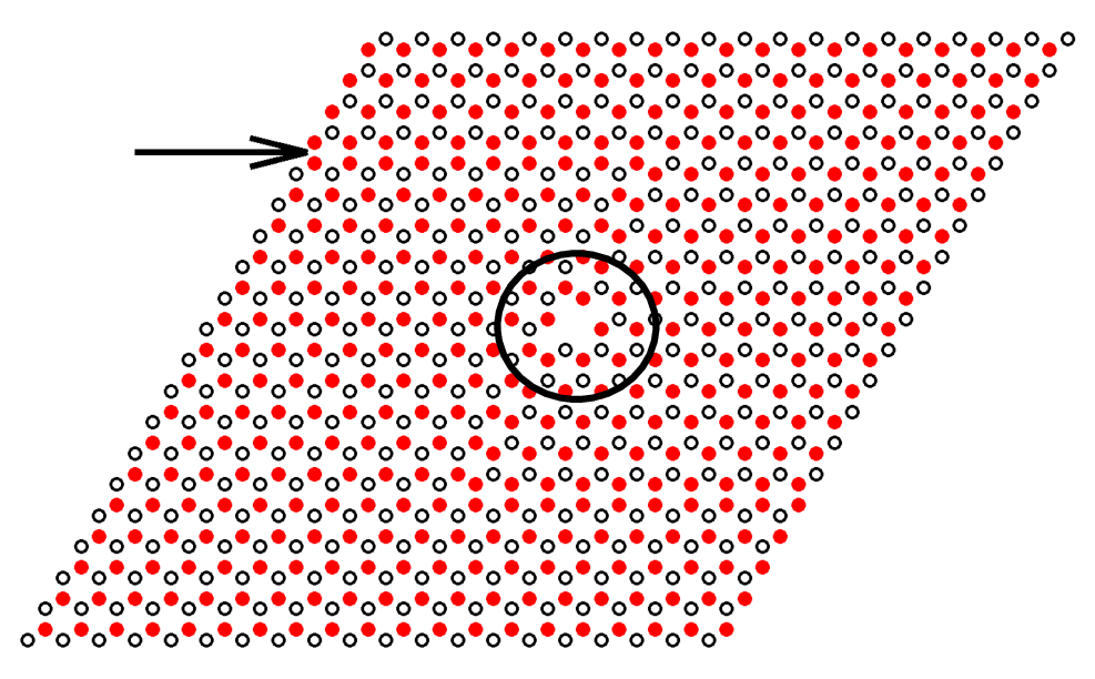
Next, we analyze the dynamic behavior at an interface between two hexagonal lattices with different unit cells. The unit cells on one side of the interface have mass parameter and the unit cells on the other side have mass parameter . These two lattices thus have the same bulk band structure. Similar to the case, we label a unit cell of type or when or , respectively. A strip, infinite along and finite along and consists of unit cells of each type is considered for our calculations. Figure 5 displays a schematic of part of the strip, along with the interface and a part of the unit cell. The interface is located along a line parallel to the direction, while the unit cell is a strip parallel to the direction as sketched in the schematic. Note that the unit cell is periodic only along the direction. As in the 1D case, two types of interfaces can be constructed, with the interface having connecting two light or two heavy masses. These two interfaces are denoted as ‘L’ and ‘H’ respectively. An example of an ‘L’ interface is illustrated in Fig. 5, where the light masses are denoted as solid red circles, while the heavy masses are denoted as empty circles.


The band structure is evaluated by fixing the masses at the left and right boundaries. Figure 5 displays the band diagrams for an ‘L’ interface and for and (or equivalently, and ). The diagram features two sets of bulk modes (black solid lines), along with two sets of modes within the bulk bandgap. These modes within the bandgap are localized modes either at the fixed ends or at the interface. The type of boundary where the mode localizes can be determined by examining the corresponding eigenvectors, which decay rapidly away from the boundary. The blue (thick solid) curve is associated with two overlapping frequencies corresponding to a localized mode at each end of the strip. Note that the two ends are locally identical, which results in this degeneracy of localized modes. The branch denoted by the dashed red line is a single mode localized at the interface. In addition, a third branch is observed above the bulk optical band, illustrated in red dashed (light) color in the figure. The eigenvector associated with this mode is also localized at the interface. However, note that it is hard to excite this mode in practice as the frequency it spans also has a wide spectrum of bulk bands.
We now consider a strip characterized by a ‘H’ type interface, i.e. with two heavy masses adjacent to each other at the interface. The mass is kept the same, while is reversed in sign compared to the previous case. Figure 5 displays the dispersion diagram for this interface, having a different set of localized modes within the bulk bandgap. Here the mode localized at the interface, shown again in dashed red (light) color starts from the bulk acoustics band, in contrast with the previous case. Furthermore, the two localized modes at the boundaries also have different frequencies, as there are now light masses at each boundary. Note also that there is an additional interface localized mode which has shifted downward below the acoustic band.


To verify the observations based on the above dispersion analysis, we conduct transient simulations on a finite lattice of unit cells. Both types and of unit cells are in the lattice, separated by a zig-zag interface of the ‘L’ type (see Fig. 6). The excitation is a -cycles sinusoidal force of frequency modulated by a Hanning window and applied to one of the interface masses along the lower right boundary, shown by an arrow in the schematic. The response of the lattice is evaluated through numerical integration of the equation of motion for the finite system considered. Figure 6 displays the amplitude of the displacements in the lattice at distinct time instants. Initially, at in Fig. 6, the wave travels along the straight portion of the interface and does not propagate into the interior or along the boundaries of the lattice. This solution is consistent with the dispersion analysis which predicts only a localized interface mode at frequency . As time progresses ( in Fig. 6), the wave bends around the zig-zag edges without any back-scattering. The wave is immune to localization and experiences negligible backscattering even as it navigates multiple bends as clearly shown from the displacement amplitude contours at (Fig. 6). After the wave hits the other boundary, it reflects and traverses in the opposite direction, as it is not immune to backscattering at the boundary, where mode hybridization occurs. We note that this response is consistent with the behavior observed for other classical analogues of the quantum Hall effect, which are also immune to backscattering only in the presence of a certain class of defects that do not cause the modes at the two valleys to hybridize.
3 Edge Waves in Continuous Elastic Plates
The concepts illustrated in the previous sections for discrete lattices are now extended to the case of an elastic plate carrying an array of resonators arranged in a hexagonal lattice topology. Thus, we seek to investigate the existence edge waves in a physical substrate, i.e. the elastic plates, that are described as a continuous elastic system.


The proposed configuration is based on the observation of Dirac cones in a plate with resonators placed in a hexagonal lattice arrangement [32]. Breaking inversion symmetry within the unit cell can be simply achieved by considering different masses for the two resonators. Figure 7 displays a schematic of the plate with two kinds of resonators, along with a zoomed-in view showing a unit cell with two resonators. The dashed lines are only to clearly depict the hexagonal geometry and are not associated with any physical features. Similar to the discrete case, breaking inversion symmetry while preserving symmetry leads to a bandgap in place of a Dirac point.
3.1 Plate Configuration and Governing Equations
We consider a thin plate of Young’s modulus , Poisson’s ratio , thickness and density . The resonators interact with the plate through a spring of stiffness and are located at positions . Also, let be the length of a unit cell of this hexagonal lattice, leading to a distance between nearest neighbor resonators.
Let and denote, respectively, the transverse displacement of the plate at point and the displacement of the resonator of type located at . The governing equations are then given by [31]
| (11a) | |||
| (11b) | |||
with being the plate bending stiffness. Similar to the discrete case, the resonator masses at the two lattice sites are expressed as and . For convenience, the following normalized frequency is introduced:
Also, the mass of the resonators is expressed in terms of the mass ratio , given by [32]
where is the area of a unit cell. For all the calculations in this work, we use the resonator properties are obtained by considering and a baseline resonance frequency [32].
3.2 Analysis of Plate Dispersion
The dispersion properties of the plate are obtained through the application of the plane wave expansion method (PWEM) [31], which expresses the plate displacement in terms of a finite number of orthogonal modes as
with being the coefficient associated with the mode . Note that the basis vectors for the modes are reciprocal lattice vectors and are hereafter denoted by the set , which contains terms of the form . The displacement field may then be written as . Similarly, using Floquet Bloch theory, the displacement of a resonator located at can be expressed as . Substituting these expressions into the plate governing equation and using the normalizing variables defined above leads to the following equation
| (12) |
Multiplying by , integrating over one unit cell and applying orthogonality gives
| (13) |
Note that the index takes values and corresponding to the two resonators within a unit cell. Similarly, substituting the displacement fields in Eqn. (11) for the resonator gives:
| (14) |
Equations (13) and (14) define an eigenvalue problem for every wave vector . The resulting eigenvalues and eigenvectors yield the frequency and the associated displacement field.

Figure 8 displays the plate dispersion diagram for two kinds of resonator unit cells. The dashed curves show the frequency for a unit cell having both masses equal , while the solid curves are the dispersion diagrams for a unit cell having dissimilar masses in the resonators (). As shown by Torrent and coworkers [32], when the resonator masses are identical, there is a Dirac cone at the point. In contrast, when the two masses are different, a bandgap forms, which essentially replicates the behavior of the discrete 2D lattice previously examined.
The nontrivial nature of the bandgaps is characterized by the valley Chern number, which is calculated by a similar approach used for the discrete lattice. To this end, the eigenvalue problem defined by Eqns. (13) and (14) is expressed as , where is a generalized displacement eigenvector and where and are the generalized mass and stiffness matrix operators, given by the coefficients of and , respectively, in these equations. Although the number of bands obtained in the solution depend on the number of terms used in the plane wave expansion, the frequencies of the first two bands are well separated from the remaining bands and their contribution to the Berry curvature is negligible as evident from the denominator term of Eqn. (10). Thus, only the two lowest bands having eigenvalues and associated eigenvectors are used for calculating the Berry curvature and Eqn. (10) for the first band having eigenvector reduces to
| (15) |
To evaluate the derivatives of the generalized stiffness with respect to the wave vector components, observe that only the first term in Eqn. (13) depends on and all other terms in the eigenvalue problem (Eqns. (13) and (14)) are independent of the wave-vector. Thus the derivative of the stiffness matrix has nonzero components only due to the diagonal terms , arising from the reciprocal lattice vectors . In particular, the nonzero component of associated with the -th component of is . Using this expression and the solution of the eigenvalue problem which yields the eigenvalues of the first two bands and their associated eigenvectors, the Berry curvature associated with each band over the entire Brillouin zone can be evaluated.


Figure 9 displays the Berry curvature associated with the first band for a plate with and it is localized near the and points. Similar to the discrete case, where it also has opposite signs at the and points. The valley Chern number associated with these two valleys are and , respectively. Similarly, for the second band, the valley Chern numbers at the and points are flipped in sign as the sum of Chern numbers over the two bands is zero. The nontrivial value of Chern numbers thus predicts the presence of topologically protected valley edge modes at the interface between two lattices whose corresponding valleys have opposite Chern numbers. Two such lattices are constructed by simply flipping the values of the two masses and leading to a different kinds of unit cell. Thus at the interface between two lattices, one having (or ) and the other having (or ) unit cells, topologically protected valley edge modes exist due to the nontrivial topology associated with the bands. For additional insight into the nature of the eigenmodes at the valley points, we examine their phases. Figure 9 displays the dispersion diagram over the and the boundaries of Brillouin zone. The insets show the phase of the displacement field for each of the eigenmodes at the and points. The polarization plots show that although the eigenvalues are identical, the eigenmodes have opposite polarizations at the and points for each band. Similar polarization reversal is observed in photonic crystals [29].
3.3 Finite Strip Dispersion Analysis and Finite Lattice Simulations
The predictions from the dispersion analysis above are verified through the dispersion analysis extended to a finite strip with an interface, along with simulation results of the response of finite plates. The dispersion diagrams for a strip are presented, similar to the previous discrete case, followed by multiple scattering simulations of a finite lattice which illustrate wave transmission along an interface even in the presence of defects.
For convenience in dispersion calculations on a strip, the lattice vectors are chosen to be orthogonal, given by and . Each lattice unit cell has resonators for this choice of lattice vectors. A strip of unit cells along the direction is considered for the study. The length of the strip is chosen to be in the vertical direction. Note that we have chosen the plate to be one unit cell longer than the zone of resonators on either side.
Consider the set of resonator displacements in the lattice described by , where the index runs from to for all the resonators in the strip . A plane wave solution in the -direction is imposed of the form
| (16) |
for the plate, where . Note that in contrast with the infinite lattice, only the -direction is periodic, and the goal is to obtain the corresponding set of functions from an eigenvalue problem for assigned . Substituting it into the governing equation, multiplying both sides by and integrating over the strip leads to the following equation for each reciprocal lattice vector and wavenumber
| (17) |
Similarly, the resonator equation becomes
| (18) |
with the first term within brackets taking values or depending on the resonator type. The above system of equations define an eigenvalue problem with eigenvalue and eigenvector having functions . It is solved numerically using beam finite elements using the procedure described in the appendix A.


We now consider a strip of unit cells with and two types of lattice configurations, which result in distinct kinds of lattice interface, similar to the discrete lattice case. Again, by virtue of bulk-boundary correspondence principle, topologically protected edge modes are guaranteed to exist at the interface between the two lattice types which have distinct valley Chern numbers. Note that the dispersion relation of a plate is . For a waveguide along the -direction, the allowable frequencies are since . In the presence of resonators, this relation becomes periodic with a period in , which is indicated by the dashed red curves in the figure. Thus only the range of frequencies enclosed between these two dashed lines are admissible for waveguiding along -direction in a plate.
We first consider the case where the lattice is in a similar configuration to an interface denoted as ‘L’ in the discrete case, with unit cells of each lattice type in a strip. Figure 10 displays a schematic of the unit cell. It has two adjacent resonators with light masses at the interface, separated by a distance . Figure 10 displays the corresponding dispersion diagram and it has two sets of bulk bands with an edge mode between them. The edge mode present in the bandgap frequencies is associated with an eigenvector localized at the interface and is illustrated by its displacement amplitude contours in Fig. 10, here calculated for .
Figure 10 displays the dispersion diagram for the strip having the an interface ‘H’, i.e. with two adjacent heavier masses separated by a distance . Similar to the previous case, we observe a mode in the bulk bandgap. The frequency of this mode has a local minimum at . Note that this mode is different from the localized mode at the interface between adjacent light masses. Indeed, comparing the frequencies associated with these two interface localized modes, we see that the ‘L’ interface is characterized by a localized mode spanning between the and valleys in the optical band and has a peak frequency at , while in the ‘H’ interface, the band associated with the localized mode spans the two valleys in the acoustic band. This feature is similar to the valley edge modes observed by Ma and Shvets [28] in photonic crystals. In contrast with the discrete case, only a light mass at the end (last resonator) results in a localized defect mode at the boundary. The boundary has been modified here to have only heavy masses at both ends and so that no modes are localized at the domain outer boundary. The eigenmodes corresponding to the edge modes in the two lattice configurations are displayed in Figs. 10 and 10 at wavenumber . The displacement amplitude in the plate strip are localized at the interface and verify our assertion of an interface mode. Note that the two modes are different and the amplitude is localized at the resonator having lower mass.
Since these modes at the interface arise due to bands on either side of the interface having distinct topological indices (valley Chern number), they are immune to backscattering and localization in the presence of a class of defects, which do not cause hybridization of the two distinct valley modes. In contrast, the localized modes present at the boundary of the strip are defect modes which lack topological protection and are susceptible to localization at corners and defects. We support these assertions through numerical simulations on an infinite plate featuring a finite resonator array. Multiple scattering simulations are conducted following the procedure described in [32] to predict displacement field in the plate resulting from a point source excitation. Note that the method yields the steady state solution after all the transients have died out.
Figure 11 displays a schematic of the problem setup with two types of unit cells in the lattice separated by a -shaped interface. The unit cells below the interface are of type , with , while those above the interface have and there are two adjacent light masses at the interface. The results are presented here for a lattice with mass parameter . Figure 12 illustrates the contours of displacement amplitude in the plate due to a point source placed on the left edge at the boundary between the two unit cell types and oscillating at a normalized frequency . The results clearly illustrate how the displacement is localized along the -shaped interface. The surrounding plate without resonators does not have a bandgap, and allows the energy to leak from the two ends of the channel into its unbounded domain. Note that there is no localization of energy even as the wave bends around corners. Furthermore, the wave amplitude is almost identical at the left and right boundary, which shows that there is no significant backscattering.
We now show the results for two further kinds of lattice imperfections. The first lattice imperfection involves removing both the resonators from a single unit cell. Figure 11 displays a schematic of this plate with defects. It is identical to the previous case, except the removal of two resonators lying in the middle section of the Z-shaped interface. Figure 13 illustrates the amplitude of the displacement field under a similar external excitation condition, with a point source placed at the interface on the left edge. We observe a robust propagation of waves even in the presence of this defect, thereby demonstrating immunity of the interface mode. Note that in contrast, in an ordinary bandgap in a lattice, removal of a unit cell may result in localized modes or it may induce strong backscattering effects. An example of such localization is shown by results obtained for a second lattice imperfection, which considers a lattice made of the same kind of unit cells () with a layer of unit cells removed along the same Z-shaped strip. Figure 13 illustrates the resulting displacement field which is strongly localized near the source and does not propagate into the channel. This localization happens because the defect is not wide enough compared to the wavelength associated with this frequency, causing the mode to hybridize with the evanescent mode in the direction normal to the channel.



4 Conclusions
This study illustrates how breaking parity or inversion symmetry within the unit cell can lead to topologically non-trivial bandgaps in both and mechanical lattices. These lattices are solely made of passive components and are characterized by a behavior which is analogous to the quantum valley Hall effect, whereby difference in valley Chern numbers at various points in the Brillouin zone are pursued and exploited. The discrete lattices are extended to an elastic plate having resonators arranged in a hexagonal array. Similar ideas of breaking inversion symmetry while preserving symmetry within the unit cell through proper choice of the resonators leads to non-trivial bandgaps in the plate.
Theoretical predictions are verified through both dispersion analyses on extended unit cells and numerical simulations on finite lattices. The dispersion studies on finite strips show the presence of edge modes localized at the interface between two distinct lattice unit cell types. Transient simulations on the discrete hexagonal lattice show wave propagation along predefined interfaces even in the presence of multiple bends. Finally, multiple scattering simulations illustrate robust edge wave propagation in plates with resonators at a Z-shaped interface even in the presence of defects.
Acknowledgments
This work is supported by a from the Air Force Office of Scientific Research (Grant Number: FA9550-13-1-0122).
Appendix A Finite element formulation for plate strip dispersion analysis
The system of equations given by Eqns. (17) and (18) define an eigenvalue problem with eigenvalue and eigenvector having functions . The solution is conducted by discretizing the above equations through two-node Hermitian finite elements [40]. The shape functions are chosen to be localized about the resonators to evaluate the force on resonators accurately. Note that they satisfy a partition of unity rule, i.e., , where is the Kroneker delta product. The solution field is expressed in terms of the displacement values of the degrees of freedom as
Substituting the above equation into the variational form of the plate equations leads to an eigenvalue problem in algebraic form, which is here solved for , with thus taking three values. The matrix form of this eigenvalue problem may then be expressed as
| (19) |
with the lower triangular entries in the stiffness matrix on the left being Hermitian conjugates of the corresponding upper triangular entries.
The expressions for the various matrices are of the form
Note that is the -th basis vector in the plane wave expansion of the plate strip. Traction free boundary conditions are used at the two ends of the strip for our calculations.
References
- [1] MZ Hasan and CL Kane. Colloquium: topological insulators. Reviews of Modern Physics, 82(4):3045, 2010.
- [2] FDM Haldane. Model for a quantum hall effect without landau levels: Condensed-matter realization of the “parity anomaly”. Physical Review Letters, 61(18):2015, 1988.
- [3] Z Yang, F Gao, X Shi, X Lin, Z Gao, Y Chong, and B Zhang. Topological acoustics. Physical review letters, 114(11):114301, 2015.
- [4] V Peano, C Brendel, M Schmidt, and F Marquardt. Topological phases of sound and light. arXiv preprint arXiv:1409.5375, 2014.
- [5] V Peano, M Houde, C Brendel, F Marquardt, and AA Clerk. Topological phase transitions and chiral inelastic transport induced by the squeezing of light. Nature communications, 7, 2016.
- [6] BG Chen, B Liu, AA Evans, J Paulose, I Cohen, V Vitelli, and CD Santangelo. Topological mechanics of origami and kirigami. Physical review letters, 116(13):135501, 2016.
- [7] DM Sussman, O Stenull, and TC Lubensky. Topological boundary modes in jammed matter. arXiv preprint arXiv:1512.04480, 2015.
- [8] FDM Haldane and S Raghu. Possible realization of directional optical waveguides in photonic crystals with broken time-reversal symmetry. Physical review letters, 100(1):013904, 2008.
- [9] L Lu, JD Joannopoulos, and M Soljacic. Topological photonics. Nature Photonics, 8:821–829, 2014.
- [10] DZ Rocklin, BG Chen, M Falk, V Vitelli, and TC Lubensky. Mechanical weyl modes in topological maxwell lattices. Physical review letters, 116(13):135503, 2016.
- [11] R Süsstrunk and SD Huber. Classification of topological phonons in linear mechanical metamaterials. arXiv preprint arXiv:1604.01033, 2016.
- [12] S Ryu, AP Schnyder, A Furusaki, and AWW Ludwig. Topological insulators and superconductors: tenfold way and dimensional hierarchy. New Journal of Physics, 12(6):065010, 2010.
- [13] E Prodan and C Prodan. Topological phonon modes and their role in dynamic instability of microtubules. Physical review letters, 103(24):248101, 2009.
- [14] P Wang, L Lu, and K Bertoldi. Topological phononic crystals with one-way elastic edge waves. Phys. Rev. Lett., 115:104302, Sep 2015.
- [15] T Kariyado and Y Hatsugai. Manipulation of dirac cones in mechanical graphene. Scientific reports, 5, 2015.
- [16] LM Nash, D Kleckner, A Read, V Vitelli, AM Turner, and WTM Irvine. Topological mechanics of gyroscopic metamaterials. Proceedings of the National Academy of Sciences, 112(47):14495–14500, 2015.
- [17] AB Khanikaev, R Fleury, SH Mousavi, and A Alù. Topologically robust sound propagation in an angular-momentum-biased graphene-like resonator lattice. Nature communications, 6, 2015.
- [18] N Swinteck, S Matsuo, K Runge, JO Vasseur, P Lucas, and PA Deymier. Bulk elastic waves with unidirectional backscattering-immune topological states in a time-dependent superlattice. Journal of Applied Physics, 118(6):063103, 2015.
- [19] R Süsstrunk and SD Huber. Observation of phononic helical edge states in a mechanical’topological insulator’. Science, 349(6243):47–50, 2015.
- [20] SH Mousavi, AB Khanikaev, and Z Wang. Topologically protected elastic waves in phononic metamaterials. Nature communications, 6, 2015.
- [21] C He, X Ni, H Ge, XC Sun, YB Chen, MH Lu, XP Liu, L Feng, and YF Chen. Acoustic topological insulator and robust one-way sound transport. arXiv preprint arXiv:1512.03273, 2015.
- [22] RK Pal, M Schaeffer, and M Ruzzene. Helical edge states and topological phase transitions in phononic systems using bi-layered lattices. Journal of Applied Physics, 119(8):084305, 2016.
- [23] G Salerno, A Berardo, T Ozawa, HM Price, L Taxis, NM Pugno, and I Carusotto. Spin-orbit coupling in a hexagonal ring of pendula. arXiv preprint arXiv:1609.09651, 2016.
- [24] J Ningyuan, C Owens, A Sommer, D Schuster, and J Simon. Time-and site-resolved dynamics in a topological circuit. Physical Review X, 5(2):021031, 2015.
- [25] S McHugh. Topological insulator realized with piezoelectric resonators. Physical Review Applied, 6(1):014008, 2016.
- [26] A Rycerz, J Tworzydło, and CWJ Beenakker. Valley filter and valley valve in graphene. Nature Physics, 3(3):172–175, 2007.
- [27] D Xiao, W Yao, and Q Niu. Valley-contrasting physics in graphene: magnetic moment and topological transport. Physical Review Letters, 99(23):236809, 2007.
- [28] T Ma and G Shvets. All-si valley-hall photonic topological insulator. New Journal of Physics, 18(2):025012, 2016.
- [29] X Chen, M Chen, and J Dong. Valley-contrasting orbital angular momentum in photonic valley crystals. arXiv preprint arXiv:1606.08717, 2016.
- [30] J Lu, C Qiu, M Ke, and Z Liu. Valley vortex states in sonic crystals. Physical review letters, 116(9):093901, 2016.
- [31] Y Xiao, J Wen, and X Wen. Flexural wave band gaps in locally resonant thin plates with periodically attached spring–mass resonators. Journal of Physics D: Applied Physics, 45(19):195401, 2012.
- [32] D Torrent, D Mayou, and J Sánchez-Dehesa. Elastic analog of graphene: Dirac cones and edge states for flexural waves in thin plates. Physical Review B, 87(11):115143, 2013.
- [33] E Andreassen, K Manktelow, and M Ruzzene. Directional bending wave propagation in periodically perforated plates. Journal of Sound and Vibration, 335:187–203, 2015.
- [34] M Oudich, M Senesi, MB Assouar, M Ruzenne, JH Sun, B Vincent, Z Hou, and TT Wu. Experimental evidence of locally resonant sonic band gap in two-dimensional phononic stubbed plates. Physical Review B, 84(16):165136, 2011.
- [35] MI Hussein, MJ Leamy, and M Ruzzene. Dynamics of phononic materials and structures: Historical origins, recent progress, and future outlook. Applied Mechanics Reviews, 66(4):040802, 2014.
- [36] M Xiao, ZQ Zhang, and CT Chan. Surface impedance and bulk band geometric phases in one-dimensional systems. Physical Review X, 4(2):021017, 2014.
- [37] J Zak. Berry’s phase for energy bands in solids. Physical review letters, 62(23):2747, 1989.
- [38] M Xiao, G Ma, Z Yang, P Sheng, ZQ Zhang, and CT Chan. Geometric phase and band inversion in periodic acoustic systems. Nature Physics, 11(3):240–244, 2015.
- [39] CL Kane and EJ Mele. Quantum spin hall effect in graphene. Physical review letters, 95(22):226801, 2005.
- [40] RD Cook et al. Concepts and applications of finite element analysis. John Wiley & Sons, 2007.