跳到论文正文
W Papers独立论文阅读器 arXiv:1611.08811 论文正文 计算阅读时间 · 0%
引用这篇论文根据当前论文元数据生成,正式投稿前建议核对。


License: arXiv.org perpetual non-exclusive license
arXiv:1611.08811v2 [cs.IT] 15 Dec 2016

Learning-Based Coexistence in Two-Tier Heterogeneous Networks with Cognitive Small CellsThanks: Lin Zhang, Guodong Zhao, Wenli Zhou, Gang Wu, Ying-Chang Liang, and Shaoqian Li are with the National Key Lab of Science and Technology on Communications, University of Electronic Science and Technology of China, Chengdu, China, emails: linzhang1913@gmail.com, gdngzhao@gmail.com, di_\_di_\_zhou@163.com, wugang99@uestc.edu.cn, liangyc@ieee.org, and lsq@uestc.edu.cn; Guodong Zhao is also with Department of Electrical and Computer Engineering, Lehigh University, Bethlehem, PA, USA.

Lin Zhang, , Guodong Zhao, , Wenli Zhou, Gang Wu, , Ying-Chang Liang, , and Shaoqian Li Affiliation:
Abstract

We study the coexistence problem in a two-tier heterogeneous network (HetNet) with cognitive small cells. In particular, we consider an underlay HetNet, where the cognitive small base station (C-SBS) is allowed to use the frequency bands of the macro cell with an access probability (AP) as long as the C-SBS satisfies a preset interference probability (IP) constraint at macro users (MUs). To enhance the AP (or transmission opportunity) of the C-SBS, we propose a learning-based algorithm for the C-SBS and exploit the distance information between the macro base station (MBS) and MUs. Generally, the signal from the MBS to a specific MU contains the distance information between the MBS to the MU. We enable the C-SBS to analyze the MBS signal on a target frequency band, and learn the distance information between the MBS and the corresponding MU. With the learnt distance information, we calculate the upper bound of the probability that the C-SBS may interfere with the MU, and design an AP with a closed-form expression under the IP constraint. Numerical results indicate that the proposed algorithm outperforms the existing methods up to 60%60\% AP (or transmission opportunity).

Index Terms:
Access probability, cognitive small cells, interference probability, learning, underlay HetNet.

I Introduction

Recent years have witnessed an explosive growth of the wireless data traffic driven by mobile devices such as smart phones and tablets [1, 2]. To accommodate the tremorous data traffic, mobile operators are pushed to increase the network capacity. However, the existing cellular architecture is designed to provide wide area coverage of users and has limited network capacity. To deal with this issue, the concept of heterogeneous network (HetNet) is proposed by embedding the conventional macro cell with multiple small cells [3, 4, 5, 6, 7, 8]. Within a HetNet, a macro base station (MBS) is equipped in the macro cell to provide wide area coverage of users. Meanwhile, a small base station (SBS) in each small cell is responsible for providing high data rate access for the users within its coverage. Consequently, the HetNet is able to provide both wide area coverage and high network capacity, and is a promising candidate for the next generation of wireless communications.

In the deployment of the HetNet, one of the major challenges is the coexistence issue between small cells and the macro cell. Among the previous works in [9, 10, 11, 12, 13, 14], there are mainly two categories of coexistence schemes. The first one is overlay HetNet [9, 10, 11], in which frequency resource is divided into two non-overlapped groups. Then, small cells and the macro cell use orthogonal frequency bands to avoid the co-channel interference, but this is inefficient in terms of spectrum efficiency, especially under a sparse small cell deployment. The second one is underlay HetNet [12, 13, 14], in which small cells and the macro cell share the same frequency bands. Then, the underlay HetNet can provide higher spectrum efficiency compared with the overlay HetNet. Nevertheless, a centralized coordinator is expected to manage the co-channel interference between small cells and the macro cell, and raises extra cost.

To deal with the coexistence issue in the HetNet, cognitive techniques are introduced to small cells, namely, cognitive small cells, in which the SBS is equipped with the cognitive capability, namely, cognitive SBS (C-SBS). In particular, the C-SBS is able to learn the status of the frequency bands in the macro cell. Then, the C-SBS can determine whether to access a frequency band or not. There are many contributions on the HetNet with cognitive small cells, e.g., [15, 16, 17, 18, 19, 20, 21]. Specifically, [15, 16, 17] investigated the overlay HetNet and proposed a two-phase opportunistic spectrum access scheme. With this scheme, the C-SBS conducts spectrum sensing on a target frequency band in the first phase. If the frequency band is idle, the C-SBS accesses the frequency band in the second phase. Otherwise, the C-SBS accesses another frequency band or keeps silent. Although the C-SBS and the MBS share the same frequency bands, they use these frequency bands in orthogonal time slots. Then, the co-channel interference from the C-SBS to MUs can be avoided. However, the C-SBS may have rare access opportunities when idle frequency bands are limited, for instance, the traffic load of the macro cell is heavy. [18, 19, 20, 21] investigated the underlay HetNet, where the C-SBS is allowed to share the same frequency bands with the MBS in the same time slots. In particular, [18, 19, 20] adopted the independent stationary point process to model the locations of MUs and designed variable access policies to the busy frequency bands under different criterion, e.g., outage probability, throughput, and spectrum efficiency. [21] developed algorithms to detect whether a specific MU is inside the C-SBS coverage and designed an access probability (AP) to the frequency band occupied by the MU under an interference probability (IP) constraint.

From [18, 19, 20, 21], we notice that the instantaneous location information of a MU is crucial for the C-SBS to maximize the AP (or transmission opportunity) in the underlay HetNet. In particular, with the instantaneous location information, the C-SBS can access the frequency band when the MU is outside the C-SBS coverage, or the C-SBS can access the frequency band with an AP to satisfy the IP constraint when the MU is inside the C-SBS coverage. On the contrary, without the instantaneous location information, the C-SBS has to consider the worst case and conservatively access the frequency band all the time. This inevitably compromises the AP (or transmission opportunity) of the C-SBS. However, the instantaneous location information of the MU is only available at the MBS and the MU, and is unknown at the C-SBS. Thus, it is challenging for the C-SBS to obtain the instantaneous location information of MUs and maximize the AP (or transmission opportunity).

One straightforward alternative is to utilize the stochastic location information of MUs in [18, 19, 20] and another approach is to utilize partial instantaneous location information of MUs in [21]. However, both schemes provide limited AP (or transmission opportunity) for the C-SBS. In this paper, we propose a learning-based algorithm for the C-SBS and exploit the MBS-MU distance information to enhance the AP (or transmission opportunity). To our best knowledge, this is the first work to enable the C-SBS to learn the MBS-MU distance information and design the AP for the C-SBS to realize the underlay HetNet. To highlight our contributions, we summarize this paper as follows:

∙\bullet We propose a learning-based method for the C-SBS and exploit the MBS-MU distance information to enhance the AP (transmission opportunity) in the underlay HetNet.

∙\bullet By enabling the C-SBS to analyze the MBS signal, we learn the MBS-MU distance information, i.e., the relation between the MBS-MU distance and the received signal-to-noise ratio (SNR) of the MBS signal at the C-SBS.

∙\bullet Based on the learnt MBS-MU distance information, we calculate the upper bound of the probability that the C-SBS may interfere with the MU. Then, we design an AP for the C-SBS with a closed-form expression under the IP constraint at the MU.

∙\bullet We numerically verify that the proposed algorithm outperforms the existing methods up to 60%60\% AP (or transmission opportunity).

The rest of the paper is organized as follows: Section II describes the system model in this paper. Section III develops algorithms for the C-SBS to learn the MBS-MU distance information. In Section IV, we exploit the learnt MBS-MU distance information and design an AP for the C-SBS u nder the IP constraint. Section V provides numerical results and compares the proposed algorithm with the state of arts. Finally, Section VI concludes the paper.

II System Model

We consider a HetNet model in Fig. 1, which consists of a macro cell with radius RR and a cognitive small cell with radius rr. In particular, MUs are uniformly distributed in the macro cell and the MBS serves each MU with a certain frequency band. Meanwhile, the C-SBS is in the coverage of the MBS and is allowed to access the frequency band being occupied by a MU for coexistence. We denote the distance from the MBS to a MU and the C-SBS as d0d_{0} and d1d_{1}, respectively. In what follows, we provide the channel model and the signal model, respectively.

Refer to caption
Figure 1: HetNet model, which consists of a macro cell with radius RR and a cognitive small cell with radius rr. In particular, MUs are uniformly distributed in the macro and the MBS serves each MU with a certain frequency band. Meanwhile, the C-SBS is in the coverage of the MBS and is allowed to access the frequency band being occupied by a MU for coexistence.

II-A Channel Model

We denote h0h_{0} (h1h_{1}), gs0g_{s_{0}} (gs1g_{s_{1}}), and g0g_{0} (g1g_{1}) as the fading, the shadowing, and the path-loss coefficients between the MBS and MU (C-SBS), respectively. Then, the channel between the MBS and the MU (C-SBS) is h0​g0​gs0{h_{0}}\sqrt{{g_{0}}{g_{s_{0}}}} (h1​g1​gs1{h_{1}}\sqrt{{g_{1}}{g_{s_{1}}}}). In particular, |hq||h_{q}| (q=0, 1q=0,\ 1) follows a Rayleigh distribution with unit mean. gsqg_{s_{q}} (q=0, 1q=0,\ 1) follows a log-normal distribution with standard derivation σs\sigma_{s}. gqg_{q} (q=0, 1q=0,\ 1) is determined by the path-loss model. If we adopt the path-loss model** * Although we adopt the path loss model (1) in this paper, our proposed algorithms can be used in other path loss models. [22]

Pl​(dq)=128+37.6​log10⁡(dq),fordq≥ξ,P_{l}(d_{q})=128+37.6\log_{10}(d_{q}),\ \ \text{for}\ \ d_{q}\geq\xi, (1)

where ξ=0.035\xi=0.035 km is the minimum distance between a transmitter and a receiver, gqg_{q} can be expressed as

gq=10−12.8​dq−3.76,fordq≥ξ.g_{q}=10^{-12.8}d_{q}^{-3.76},\ \ \text{for}\ \ d_{q}\geq\xi. (2)
Refer to caption
Figure 2: Channel model, where time axis is divided into blocks and each blocks consists of multiple subblocks. In particular, gqg_{q} remains constant all the time with a given dqd_{q}, gsqg_{s_{q}} (q=0, 1q=0,\ 1) remains constant within each block (ii) and varies independently among different blocks, and hqh_{q} (q=0, 1q=0,\ 1) remains constant within each subblock (i,ji,j) and varies among different subblocks.

For illustrations, we provide the channel model in Fig. 2, where time axis is divided into blocks and each block consists of multiple subblocks. In particular, gqg_{q} remains constant all the time for a given dqd_{q}, gsqg_{s_{q}} (q=0, 1q=0,\ 1) remains constant within each block (ii) and varies independently among different blocks, and hqh_{q} (q=0, 1q=0,\ 1) remains constant within each subblock (i,ji,j) and varies among different subblocks.

II-B Signal Model

II-B1 Signal model from the MBS to the MU

If we denote x0x_{0} as the MBS signal with unit power, i.e., |x0|2=1|x_{0}|^{2}=1, and denote p0p_{0} as the transmit power of the MBS, the received signal at the MU is

y0​(i,j)=h0​(i,j)​g0​gs0​(i)​p0​(i,j)​x0​(i,j)+n0​(i,j),y_{0}(i,j)=h_{0}(i,j)\sqrt{g_{0}g_{s_{0}}(i)p_{0}(i,j)}x_{0}(i,j)+n_{0}(i,j), (3)

where (i)(i) denotes the index of the iith block, (i,j)(i,j) represents the index of the jjth subblock in the iith block, n0n_{0} represents the AWGN at the MU with zero mean and variance σ2\sigma^{2}. Then, the SNR of the received signal at the MU is

γ0​(i,j)=|h0​(i,j)|2​g0​gs0​(i)​p0​(i,j)σ2.\gamma_{0}(i,j)=\frac{|h_{0}(i,j)|^{2}g_{0}g_{s_{0}}(i)p_{0}(i,j)}{\sigma^{2}}. (4)

We further consider that the MBS and the MU adopt close loop power control (CLPC) to provide quality of service (QoS) guaranteed wireless communication [23, 24]. That is, the MBS automatically adjusts its transmit power to meet a certain target SNR γT\gamma_{T} at the MU. Then, the transmit power of the MBS is

p0​(i,j)=γT​σ2|h0​(i,j)|2​g0​gs0​(i).p_{0}(i,j)=\frac{{\gamma_{T}\sigma^{2}}}{{|h_{0}(i,j)|^{2}{g_{0}g_{s_{0}}(i)}}}. (5)

II-B2 Signal model from the MBS to the C-SBS

In the meantime, the received MBS signal at the C-SBS is

y1​(i,j)=h1​(i,j)​g1​gs1​(i)​p0​(i,j)​x0​(i,j)+n1​(i,j),y_{1}(i,j)=h_{1}(i,j)\sqrt{{g_{1}}{g_{s_{1}}(i)}{p_{0}(i,j)}}{x_{0}}(i,j)+n_{1}(i,j), (6)

where n1n_{1} is the AWGN at the C-SBS with zero mean and variance σ2\sigma^{2}. Then, the SNR of the received MBS signal at the C-SBS is

γ1​(i,j)=|h1​(i,j)|2​g1​gs1​(i)​p0​(i,j)σ2.\gamma_{1}(i,j)=\frac{{|h_{1}(i,j)|^{2}{g_{1}}{g_{s_{1}}(i)}{p_{0}(i,j)}}}{{\sigma^{2}}}. (7)

By Substituting (2) and (5) into (7), γ1​(i,j)\gamma_{1}(i,j) in (7) can be rewritten as

γ1​(i,j)=γT​d1−3.76d0−3.76​gs1​(i)gs0​(i)​|h1​(i,j)|2|h0​(i,j)|2.{\gamma_{1}}(i,j)=\frac{{{\gamma_{T}}{d_{1}^{-3.76}}}}{{{d_{0}^{-3.76}}}}\frac{g_{s_{1}}(i)}{g_{s_{0}}(i)}\frac{{|h_{1}(i,j)|^{2}}}{{|h_{0}(i,j)|^{2}}}. (8)

III MBS-MU Distance Information Learning

In this section, we develop an algorithm for the C-SBS to learn the MBS-MU distance information. In principle, when the MBS is transmitting signals to the MU with a target SNR, the transmission is based on the MBS-MU distance. In particular, if the MBS-MU distance is small, the MBS is able to satisfy the target SNR with a small transmit power. This leads to a small measured SNR at the C-SBS. Otherwise, the MBS has to increase its transmit power to achieve the target SNR. This results in a large measured SNR at the C-SBS. Therefore, the measured SNR at the C-SBS contains the MBS-MU distance information. In what follows, we will first calculate the cumulative density function (CDF) of the measured SNR, and then obtain the relation between the MBS-MU distance and the measured SNR.

III-A CDF of the SNR at the C-SBS

Removing the time index of the SNR at the C-SBS in (8) and rewriting the SNR in dB, we have

γ1,d​B=γT,d​B+37.6​log10⁡(d0d1)+θr+θs,\displaystyle{\gamma_{1,dB}}={\gamma_{T,dB}}+37.6{\log_{10}}\left(\frac{d_{0}}{d_{1}}\right)+\theta_{r}+\theta_{s}, (9)

where θr=10​log10⁡(|h1|2/|h0|2){\theta_{r}}=10{\log_{10}}\left(|h_{1}|^{2}/|h_{0}|^{2}\right) and θs=10​log10⁡(gs1)−10​log10⁡(gs0){\theta_{s}}=10{\log_{10}}\left({{g_{s_{1}}}}\right)-10{\log_{10}}\left({{g_{s_{0}}}}\right).

Then, the CDF of γ1,d​B\gamma_{1,dB} can be expressed as

FΓ1,d​B​(γ1,d​B)\displaystyle F_{\Gamma_{1,dB}}(\gamma_{1,dB})
=\displaystyle= Pr{γT,d​B+37.6log10(d0d1)+θr+θs≤γ1,d​B}\displaystyle\Pr\left\{{\gamma_{T,dB}}+37.6{\log_{10}}\left(\frac{d_{0}}{d_{1}}\right)+{\theta_{r}}+{\theta_{s}}\leq\gamma_{1,dB}\right\}
=\displaystyle= Pr{θr+θs≤γ1,d​B−γT,d​B−37.6log10(d0d1)},\displaystyle\Pr\left\{{\theta_{r}}\!+{\theta_{s}}\leq\gamma_{1,dB}\!-{\gamma_{T,dB}}\!-37.6{\log_{10}}\left(\frac{d_{0}}{d_{1}}\right)\right\}, (10)

which is related to the distributions of both θr\theta_{r} and θs\theta_{s}. In the following, we first calculate the probability density function (PDF) of both θr\theta_{r} and θs\theta_{s}, and then obtain the CDF of γ1,d​B\gamma_{1,dB} with (10).

III-A1 PDF of θr\theta_{r}

Since both |h0||h_{0}| and |h1||h_{1}| follow a Rayleigh distribution with unit mean, the CDF of ϕ=|h1|2/|h0|2\phi=|h_{1}|^{2}/|h_{0}|^{2} is [25]

FΦ​(ϕ)=ϕ1+ϕ.\displaystyle F_{\Phi}(\phi)=\frac{\phi}{1+\phi}. (11)

Then, the CDF of θr=10​log10⁡(ϕ)\theta_{r}=10\log_{10}(\phi) is

FΘr​(θr)=\displaystyle F_{\Theta_{r}}(\theta_{r})= Pr{10log10(ϕ)≤θr}\displaystyle\Pr\left\{10\log_{10}(\phi)\leq\theta_{r}\right\}
=\displaystyle= Pr{ϕ≤10θr10}\displaystyle\Pr\left\{\phi\leq 10^{\frac{\theta_{r}}{10}}\right\}
=\displaystyle= FΦ​(10θr10)\displaystyle F_{\Phi}\left(10^{\frac{\theta_{r}}{10}}\right)
=\displaystyle= 11+10−θr10.\displaystyle\frac{1}{1+10^{-\frac{\theta_{r}}{10}}}. (12)

Taking the derivation of FΘr​(θr)F_{\Theta_{r}}(\theta_{r}), we have the PDF of θr\theta_{r} as

fΘr​(θr)=ln⁡10⋅10−θr1010​(1+10−θr10)2.{f_{{\Theta_{r}}}}\left({{\theta_{r}}}\right)=\frac{{\ln 10\cdot{{10}^{-\frac{{{\theta_{r}}}}{{10}}}}}}{{10{{\left({1+{{10}^{-\frac{{{\theta_{r}}}}{{10}}}}}\right)}^{2}}}}. (13)

III-A2 PDF of θs\theta_{s}

Recall that both gs0g_{s_{0}} and gs1g_{s_{1}} follow a log-normal distribution with standard derivation σs\sigma_{s}. Then, it is straightforward to obtain that θs\theta_{s} follows a normal distribution with zero means and variance 2​σs22\sigma_{s}^{2}. Thus, the PDF of θs\theta_{s} is

fΘs​(θs)=14​π​σs2​e−θs24​σs2.{f_{{\Theta_{s}}}}\left({{\theta_{s}}}\right)=\frac{1}{{\sqrt{4\pi\sigma_{s}^{2}}}}{e^{-\frac{{{{{{\theta_{s}}}}^{2}}}}{{4{\sigma_{s}^{2}}}}}}. (14)

Based on (13) and (14), the CDF of γ1,d​B\gamma_{1,dB} in (10) can be calculated as

FΓ1,d​B​(γ1,d​B)=\displaystyle F_{\Gamma_{1,dB}}(\gamma_{1,dB})= Pr{θr+θs≤m(γ1,d​B)}\displaystyle\Pr\left\{{\theta_{r}}+{\theta_{s}}\leq m(\gamma_{1,dB})\right\}
=\displaystyle= ∫−∞∞∫−∞m⁡(γ1,d​B)−θsfΘs​(θs)​fΘr​(θr)​d​θr​d​θs\displaystyle\int_{-\infty}^{\infty}\int_{-\infty}^{m(\gamma_{1,dB})-{\theta_{s}}}\!\!f_{\Theta_{s}}\left(\theta_{s}\right)\!\!f_{\Theta_{r}}\left(\theta_{r}\right)d\theta_{r}d\theta_{s}
=\displaystyle\!=\! ∫−∞∞fΘs​(θs)​FΘr​(m⁡(γ1,d​B)−θs)​d​θs,\displaystyle\int_{-\infty}^{\infty}\!\!f_{\Theta_{s}}\left(\theta_{s}\right)F_{\Theta_{r}}\left(m(\gamma_{1,dB})\!-\!{\theta_{s}}\!\right)d\theta_{s}, (15)

where m⁡(γ1,d​B)=γ1,d​B−γT,d​B−37.6​log10⁡(d0d1)m(\gamma_{1,dB})=\gamma_{1,dB}-{\gamma_{T,dB}}-37.6{\log_{10}}\left(\frac{d_{0}}{d_{1}}\right).

III-B Relation between d0d_{0} and γ1,d​B\gamma_{1,dB}

To begin with, we provide the following definition.

Definition 1

For a random variable XX with CDF FX​(x)F_{X}(x), x∈ℝx\in\mathbb{R}, if x12x_{\frac{1}{2}} satisfies both FX(x12)=Pr{X≤x12}=12F_{X}(x_{\frac{1}{2}})=\Pr\{X\leq x_{\frac{1}{2}}\}=\frac{1}{2} and 1−FX(x12)=Pr{X≥x12}=121-F_{X}(x_{\frac{1}{2}})=\Pr\{X\geq x_{\frac{1}{2}}\}=\frac{1}{2}, x12x_{\frac{1}{2}} is defined as the median of the random variable XX.

If we denote the median of the random variable γ1,d​B\gamma_{1,dB} as γ1,d​B,12\gamma_{1,dB,\frac{1}{2}}, we have the following lemma.

Lemma 1

The median of the random variable γ1,d​B\gamma_{1,dB} is γ1,d​B,12=γT,d​B+37.6​log10⁡(d0d1)\gamma_{1,dB,\frac{1}{2}}={\gamma_{T,dB}}+37.6{\log_{10}}\left(\frac{d_{0}}{d_{1}}\right).

Proof:

The detailed proof of this Lemma is provided in Appendix A. ∎

From Definition 1 and Lemma 1, the probability that each sample of γ1,d​B\gamma_{1,dB} is smaller or larger than γ1,d​B,12\gamma_{1,dB,\frac{1}{2}} is equal to 12\frac{1}{2}. Suppose that the C-SBS observes MBS signals in II blocks and measures γ1,d​B\gamma_{1,dB} of JJ subblocks within each block. Then, the C-SBS can obtain K=I​JK=IJ independent samples of γ1,d​B\gamma_{1,dB}, namely, γ1,d​B​(i,j)\gamma_{1,dB}(i,j) (1≤i≤I1\leq i\leq I, 1≤j≤J1\leq j\leq J). By resorting these KK samples in an ascending order, we relabel these samples as γ¯1,d​B​(k)\bar{\gamma}_{1,dB}(k) (1≤k≤K1\leq k\leq K). Then, we have the relation between the MBS-MU distance and the received SNR γ1,d​B\gamma_{1,dB} (or γ¯1,d​B\bar{\gamma}_{1,dB}) at the C-SBS in the following Theorem.

Theorem 1

Define a function f⁡(x)=d1​10x−γT,d​B37.6f(x)=d_{1}10^{\frac{x-\gamma_{T,dB}}{37.6}}. Then, for a given distance d0ed_{0}^{e} from the MBS, the probability that the distance d0d_{0} is larger than d0ed_{0}^{e} follows:

∙\bullet If d0e<f⁡(γ¯1,d​B​(1))d_{0}^{e}<f\left(\bar{\gamma}_{1,dB}(1)\right), we have

1−(1/2)K<Pr{d0e<d0}<1.1-\left(1/2\right)^{K}<\Pr\left\{d_{0}^{e}<d_{0}\right\}<1. (16)

∙\bullet If d0e≥f⁡(γ¯1,d​B​(K))d_{0}^{e}\geq f\left(\bar{\gamma}_{1,dB}(K)\right), we have

0<Pr{d0e≤d0}<(12)K.0<\Pr\left\{d_{0}^{e}\leq d_{0}\right\}<\left(\frac{1}{2}\right)^{K}. (17)

∙\bullet If f⁡(γ¯1,d​B​(k′))≤d0e<f⁡(γ¯1,d​B​(k′+1))f\left(\bar{\gamma}_{1,dB}(k^{\prime})\right)\leq d_{0}^{e}<f\left(\bar{\gamma}_{1,dB}(k^{\prime}+1)\right), where 1≤k′≤K−11\leq k^{\prime}\leq K-1, we have

(12)K(CKk′+1+CKk′+2+⋯+CKK)≤Pr{d0e≤d0}\displaystyle\left(\frac{1}{2}\right)^{K}\left(C_{K}^{k^{\prime}+1}+C_{K}^{k^{\prime}+2}+\cdots+C_{K}^{K}\right)\leq\Pr\left\{d_{0}^{e}\leq d_{0}\right\}
≤\displaystyle\leq (12)K​(CKk′+CKk′+1+⋯+CKK).\displaystyle\left(\frac{1}{2}\right)^{K}\left(C_{K}^{k^{\prime}}+C_{K}^{k^{\prime}+1}+\cdots+C_{K}^{K}\right). (18)
Proof:

The detailed proof of this Theorem is provided in Appendix B. ∎

Theorem 1 provides both the upper bound and the lower bound of the probability that the MBS-MU distance is in a certain region. With this theorem, we will design the AP of the C-SBS and satisfy the IP constraint at the MU in the next section.

IV Coexistence between the Cognitive Small Cell and the Macro cell

In this section, we utilize the learnt MBS-MU distance information, i.e., relation between d0d_{0} and γ¯1,d​B\bar{\gamma}_{1,dB}, to design the AP for the coexistence between the cognitive small cell and the macro cell. We notice that the AP design may be different for distinct locations of the C-SBS within the macro cell. Thus, we will first classify the locations of the C-SBS into three scenarios. Then, we design the AP of the C-SBS in each scenario.

IV-A Classification of Distinct Scenarios
Refer to caption
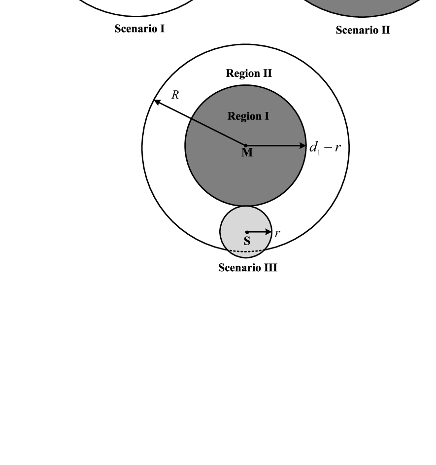
Figure 3: Illustrations of three scenarios, in which the C-SBS is in different locations within the macro cell.

Based on the MBS-C-SBS distance d1d_{1}, we consider three scenarios as shown in Fig. 3, where points “M” and “S” denote the MBS and the C-SBS, respectively.

∙\bullet In Scenario I, the MBS-C-SBS distance d1d_{1} is small, i.e., ξ≤d1≤r+ξ\xi\leq d_{1}\leq r+\xi. Then, we divide the macro cell into two non-overlapped regions†† † Since the minimum distance between a transmitter and a receiver is ξ>0\xi>0, we only consider the regions satisfying the minimum distance., i.e., Region I and Region II. In particular, Region I denotes the region where the distance from the MBS is between ξ\xi and d1+rd_{1}+r, and Region II denotes the region where the distance from the MBS is between d1+rd_{1}+r and RR.

∙\bullet In Scenario II, the MBS-C-SBS distance d1d_{1} is medium, i.e., r+ξ<d1<R−rr+\xi<d_{1}<R-r. Then, we divide the macro cell into three non-overlapped regions, i.e., Region I, Region II, and Region III. In particular, Region I denotes the region where the distance from the MBS is between ξ\xi and d1−rd_{1}-r, and Region II denotes the region where the distance from the MBS is between d1−rd_{1}-r and d1+rd_{1}+r, and Region III denotes the region where the distance from the MBS is between d1+rd_{1}+r and RR.

∙\bullet In Scenario III, the MBS-C-SBS distance d1d_{1} is large, i.e., R−r≤d1≤R+rR-r\leq d_{1}\leq R+r. Then, we divide the macro cell into two non-overlapped regions, i.e., Region I and Region II. In particular, Region I denotes the region where the distance from the MBS is between ξ\xi and d1−rd_{1}-r, and Region II denotes the region where the distance from the MBS is between d1−rd_{1}-r and RR.

IV-B AP Design in Scenario I

In this part, we exploit the results in Theorem 1 to design the AP of the C-SBS and satisfy the IP constraint at the MU in Scenario I, where the macro cell is divided into two regions. In this scenario, the C-SBS may cause interference to the MU if the MU is located in Region I, i.e., ξ≤d0≤d1+r\xi\leq d_{0}\leq d_{1}+r. According to the relation between the measured SNRs at the C-SBS and ξ\xi, ξ\xi may satisfy

0<ξ<f⁡(γ¯1,d​B​(1)),\displaystyle 0<\xi<f\left(\bar{\gamma}_{1,dB}(1)\right), (19)

or

f⁡(γ¯1,d​B​(k0))≤ξ<f⁡(γ¯1,d​B​(k0+1)),\displaystyle f\left(\bar{\gamma}_{1,dB}(k_{0})\right)\leq\xi<f\left(\bar{\gamma}_{1,dB}(k_{0}+1)\right), (20)

for 1≤k0≤K−11\leq k_{0}\leq K-1, or

f⁡(γ¯1,d​B​(K))≤ξ.\displaystyle f\left(\bar{\gamma}_{1,dB}(K)\right)\leq\xi. (21)

Meanwhile, according to the relation between the measured SNRs at the C-SBS and d1+rd_{1}+r, d1+rd_{1}+r may satisfy

0<d1+r<f⁡(γ¯1,d​B​(1)),\displaystyle 0<d_{1}+r<f\left(\bar{\gamma}_{1,dB}(1)\right), (22)

or

f⁡(γ¯1,d​B​(k2))≤d1+r<f⁡(γ¯1,d​B​(k2+1)),\displaystyle f\left(\bar{\gamma}_{1,dB}(k_{2})\right)\leq d_{1}+r<f\left(\bar{\gamma}_{1,dB}(k_{2}+1)\right), (23)

for 1≤k2≤K−11\leq k_{2}\leq K-1, or

f⁡(γ¯1,d​B​(K))≤d1+r.\displaystyle f\left(\bar{\gamma}_{1,dB}(K)\right)\leq d_{1}+r. (24)

Due to the increasing monotonicity of f⁡(x)f(x) and ξ<d1+r\xi<d_{1}+r, we have six cases of ξ\xi and d1+rd_{1}+r: Case I): ξ\xi satisfies (19) and d1+rd_{1}+r satisfies (22); Case II): ξ\xi satisfies (19) and d1+rd_{1}+r satisfies (23); Case III): ξ\xi satisfies (19) and d1+rd_{1}+r satisfies (24); Case IV) ξ\xi satisfies (20) and d1+rd_{1}+r satisfies (23); Case V) ξ\xi satisfies (20) and d1+rd_{1}+r satisfies (24); Case VI) ξ\xi satisfies (21) and d1+rd_{1}+r satisfies (24).

Next, we first calculate the probability ρI\rho_{\text{I}} that the MU is in Region I for each case and then design the corresponding AP. In the sequential, we denote SI=π​(d1+r)2−π​ξ2S_{\text{I}}=\pi(d_{1}+r)^{2}-\pi\xi^{2} as the area of Region I, and denote ScS_{\text{c}} as the area of the interference region, where the MU may appear in the C-SBS coverage. From Appendix C, we have

Sc={π​r2−π​ξ2,ξ≤d1<r−ξ,(π−φ2)r2−φ1ξ2+d1ξsinφ1,r−ξ≤d1≤r+ξ,\displaystyle S_{\text{c}}\!\!=\!\!\left\{\begin{aligned} &\!\!\pi r^{2}-\pi\xi^{2},&\!\!&\xi\leq d_{1}<r-\xi,\\ &\!\!(\pi\!-\!\varphi_{2})r^{2}\!-\!\varphi_{1}\xi^{2}\!+\!d_{1}\xi\sin\varphi_{1},&\!\!&r\!-\!\xi\!\leq\!d_{1}\!\leq\!r\!+\!\xi,\end{aligned}\right. (25)

where φ1=arccos⁡d12+ξ2−r22​d1​ξ\varphi_{1}=\arccos\frac{d_{1}^{2}+\xi^{2}-r^{2}}{2d_{1}\xi}, φ2=arccos⁡d12+r2−ξ22​d1​r\varphi_{2}=\arccos\frac{d_{1}^{2}+r^{2}-\xi^{2}}{2d_{1}r}.

IV-B1 AP Design in Case I

In this case, ξ\xi satisfies (19) and d1+rd_{1}+r satisfies (22). The probability ρI\rho_{\text{I}} that the MU is in Region I is

ρI=\displaystyle\rho_{\text{I}}= Pr{ξ≤d0≤d1+r}\displaystyle\Pr\left\{\xi\leq d_{0}\leq d_{1}+r\right\}
=\displaystyle= Pr{d0≥ξ}−Pr{d0≥d1+r}\displaystyle\Pr\left\{d_{0}\geq\xi\right\}\!-\!\Pr\left\{d_{0}\geq d_{1}+r\right\}
≤(I-a)\displaystyle\overset{\text{(I-a)}}{\leq} 1−1+(12)K\displaystyle 1-1+\left(\frac{1}{2}\right)^{K}
=\displaystyle= (12)K,\displaystyle\left(\frac{1}{2}\right)^{K}, (26)

where we use (16) in (I-a).

To control the IP constraint η\eta at the MU, the AP of the C-SBS needs to satisfy 0≤ρAP≤10\leq\rho_{\text{AP}}\leq 1 and ρAP​ρI​ScSI≤η\rho_{\text{AP}}\rho_{\text{I}}\frac{S_{\text{c}}}{S_{\text{I}}}\leq\eta, i.e., ρAP≤min⁡{η​SIρI​Sc,1}=min⁡{η⁡[π​(d1+r)2−π​ξ2]ρI​Sc,1}\rho_{\text{AP}}\leq\min\left\{\frac{\eta S_{\text{I}}}{\rho_{\text{I}}S_{\text{c}}},1\right\}=\min\left\{\frac{\eta[\pi(d_{1}+r)^{2}-\pi\xi^{2}]}{\rho_{\text{I}}S_{\text{c}}},1\right\}, which can be lower bounded by

min⁡{η⁡[π​(d1+r)2−π​ξ2]ρI​Sc,1}\displaystyle\min\left\{\frac{\eta[\pi(d_{1}+r)^{2}-\pi\xi^{2}]}{\rho_{\text{I}}S_{\text{c}}},1\right\}
≥(I-b)\displaystyle\overset{\text{(I-b)}}{\geq} min⁡{η​2K​[π​(d1+r)2−π​ξ2]Sc,1},\displaystyle\min\left\{\frac{\eta 2^{K}[\pi(d_{1}\!+\!r)^{2}-\pi\xi^{2}]}{S_{\text{c}}},1\right\}, (27)

where we use (26) in (I-b).

Thus, to protect the MU in this case, the maximum AP of the C-SBS is

ρAP=min⁡{η​2K​[π​(d1+r)2−π​ξ2]Sc,1},\displaystyle\rho_{\text{AP}}=\min\left\{\frac{\eta 2^{K}[\pi(d_{1}+r)^{2}-\pi\xi^{2}]}{S_{\text{c}}},1\right\}, (28)

where ScS_{\text{c}} is shown in (25).

IV-B2 AP Design in Case II

In this case, ξ\xi satisfies (19) and d1+rd_{1}+r satisfies (23). The probability ρI\rho_{\text{I}} that the MU is in Region I is

ρI=\displaystyle\rho_{\text{I}}= Pr{d0≥ξ}−Pr{d0≥d1+r}\displaystyle\Pr\left\{d_{0}\geq\xi\right\}-\Pr\left\{d_{0}\geq d_{1}+r\right\}
≤(I-c)\displaystyle\overset{\text{(I-c)}}{\leq} 1−(12)K​(CKk2+1+CKk2+2+⋯+CKK)\displaystyle 1-\left(\frac{1}{2}\right)^{K}\left(C_{K}^{k_{2}+1}+C_{K}^{k_{2}+2}+\cdots+C_{K}^{K}\right)
=\displaystyle= (12)K​(CK0+CK1+⋯+CKk2),\displaystyle\left(\frac{1}{2}\right)^{K}\left(C_{K}^{0}+C_{K}^{1}+\cdots+C_{K}^{k_{2}}\right), (29)

where we use (16) and (18) in (I-c).

To control the IP constraint η\eta at the MU, the AP of the C-SBS needs to satisfy 0≤ρAP≤10\leq\rho_{\text{AP}}\leq 1 and ρAP​ρI​ScSI≤η\rho_{\text{AP}}\rho_{\text{I}}\frac{S_{\text{c}}}{S_{\text{I}}}\leq\eta, i.e., ρAP≤min⁡{η​SIρI​Sc,1}=min⁡{η⁡([π​(d1+r)2−π​ξ2]CLOSEρI​Sc,1}\rho_{\text{AP}}\leq\min\left\{\frac{\eta S_{\text{I}}}{\rho_{\text{I}}S_{\text{c}}},1\right\}=\min\left\{\frac{\eta([\pi(d_{1}+r)^{2}-\pi\xi^{2}]}{\rho_{\text{I}}S_{\text{c}}},1\right\}, which can be lower bounded by

min⁡{η⁡[π​(d1+r)2−π​ξ2]ρI​Sc,1}\displaystyle\min\left\{\frac{\eta[\pi(d_{1}+r)^{2}-\pi\xi^{2}]}{\rho_{\text{I}}S_{\text{c}}},1\right\}
≥(I-d)\displaystyle\overset{\text{(I-d)}}{\geq} min⁡{η​2K​[π​(d1+r)2−π​ξ2](CK0+CK1+⋯+CKk2)​Sc,1},\displaystyle\min\left\{\frac{\eta 2^{K}[\pi(d_{1}+r)^{2}-\pi\xi^{2}]}{(C_{K}^{0}+C_{K}^{1}+\cdots+C_{K}^{k_{2}})S_{\text{c}}},1\right\}, (30)

where we use (29) in (I-d).

Thus, to protect the MU in this case, the maximum AP of the C-SBS is

ρAP=min⁡{η​2K​[π​(d1+r)2−π​ξ2](CK0+CK1+⋯+CKk2)​Sc,1},\displaystyle\rho_{\text{AP}}=\min\left\{\frac{\eta 2^{K}[\pi(d_{1}+r)^{2}-\pi\xi^{2}]}{(C_{K}^{0}+C_{K}^{1}+\cdots+C_{K}^{k_{2}})S_{\text{c}}},1\right\}, (31)

where ScS_{\text{c}} is shown in (25).

IV-B3 AP Design in Case III

In this case, ξ\xi satisfies (19) and d1+rd_{1}+r satisfies (24). The probability ρI\rho_{\text{I}} that the MU is in Region II is

ρI=Pr{d0≥ξ}−Pr{d0≥d1+r}≤(I-e)1,\displaystyle\rho_{\text{I}}=\Pr\left\{d_{0}\geq\xi\right\}-\Pr\left\{d_{0}\geq d_{1}+r\right\}\overset{\text{(I-e)}}{\leq}1, (32)

where we use (16) and (17) in (I-e).

To control the IP constraint η\eta at the MU, the AP of the C-SBS needs to satisfy 0≤ρAP≤10\leq\rho_{\text{AP}}\leq 1 and ρAP​ρI​ScSI≤η\rho_{\text{AP}}\rho_{\text{I}}\frac{S_{\text{c}}}{S_{\text{I}}}\leq\eta, i.e., ρAP≤min⁡{η​SIρI​Sc,1}=min⁡{η⁡[π​(d1+r)2−π​ξ2]ρI​Sc,1}\rho_{\text{AP}}\leq\min\left\{\frac{\eta S_{\text{I}}}{\rho_{\text{I}}S_{\text{c}}},1\right\}=\min\left\{\frac{\eta[\pi(d_{1}+r)^{2}-\pi\xi^{2}]}{\rho_{\text{I}}S_{\text{c}}},1\right\}, which can be lower bounded by

min⁡{η⁡[π​(d1+r)2−π​ξ2]ρI​Sc,1}\displaystyle\min\left\{\frac{\eta[\pi(d_{1}+r)^{2}-\pi\xi^{2}]}{\rho_{\text{I}}S_{\text{c}}},1\right\}
≥(I-f)\displaystyle\overset{\text{(I-f)}}{\geq} min⁡{η⁡[π​(d1+r)2−π​ξ2]Sc,1},\displaystyle\min\left\{\frac{\eta[\pi(d_{1}+r)^{2}-\pi\xi^{2}]}{S_{\text{c}}},1\right\}, (33)

where we use (32) in (I-f).

Thus, to protect the MU in this case, the maximum AP of the C-SBS is

ρAP=min⁡{η⁡[π​(d1+r)2−π​ξ2]Sc,1},\displaystyle\rho_{\text{AP}}=\min\left\{\frac{\eta[\pi(d_{1}+r)^{2}-\pi\xi^{2}]}{S_{\text{c}}},1\right\}, (34)

where ScS_{\text{c}} is shown in (25).

IV-B4 AP Design in Case IV

In this case, ξ\xi satisfies (20) and d1+rd_{1}+r satisfies (23). The probability ρI\rho_{\text{I}} that the MU is in Region II is

ρI=\displaystyle\rho_{\text{I}}= Pr{d0≥ξ}−Pr{d0≥d1+r}\displaystyle\Pr\left\{d_{0}\geq\xi\right\}-\Pr\left\{d_{0}\geq d_{1}+r\right\}
≤(I-g)\displaystyle\overset{\text{(I-g)}}{\leq} (12)K​(CKk0+CKk0+1+⋯+CKK)\displaystyle\left(\frac{1}{2}\right)^{K}\left(C_{K}^{k_{0}}+C_{K}^{k_{0}+1}+\cdots+C_{K}^{K}\right)
−(12)K​(CKk2+1+CKk2+2+⋯+CKK)\displaystyle-\left(\frac{1}{2}\right)^{K}\left(C_{K}^{k_{2}+1}+C_{K}^{k_{2}+2}+\cdots+C_{K}^{K}\right)
=\displaystyle= (12)K​(CKk0+CKk0+1+⋯+CKk2),\displaystyle\left(\frac{1}{2}\right)^{K}\left(C_{K}^{k_{0}}+C_{K}^{k_{0}+1}+\cdots+C_{K}^{k_{2}}\right), (35)

where we use (18) in (I-g).

To control the IP constraint η\eta at the MU, the AP of the C-SBS needs to satisfy 0≤ρAP≤10\leq\rho_{\text{AP}}\leq 1 and ρAP​ρI​ScSI≤η\rho_{\text{AP}}\rho_{\text{I}}\frac{S_{\text{c}}}{S_{\text{I}}}\leq\eta, i.e., ρAP≤min⁡{η​SIρI​Sc,1}=min⁡{η⁡[π​(d1+r)2−π​ξ2]ρI​Sc,1}\rho_{\text{AP}}\leq\min\left\{\frac{\eta S_{\text{I}}}{\rho_{\text{I}}S_{\text{c}}},1\right\}=\min\left\{\frac{\eta[\pi(d_{1}+r)^{2}-\pi\xi^{2}]}{\rho_{\text{I}}S_{\text{c}}},1\right\}, which can be lower bounded by

min⁡{η⁡[π​(d1+r)2−π​ξ2]ρI​Sc,1}\displaystyle\min\left\{\frac{\eta[\pi(d_{1}+r)^{2}-\pi\xi^{2}]}{\rho_{\text{I}}S_{\text{c}}},1\right\}
≥(I-h)\displaystyle\overset{(\text{I-h})}{\geq} min⁡{η​2K​(π⁡[π​(d1+r)2−π​ξ2]CLOSE(CKk0+CKk0+1+⋯+CKk2)​Sc,1},\displaystyle\min\left\{\frac{\eta 2^{K}(\pi[\pi(d_{1}+r)^{2}-\pi\xi^{2}]}{(C_{K}^{k_{0}}+C_{K}^{k_{0}+1}+\cdots+C_{K}^{k_{2}})S_{\text{c}}},1\right\}, (36)

where we use (35) in (I-h).

Thus, to protect the MU in this case, the maximum AP of the C-SBS is

ρAP=min⁡{η​2K​[π​(d1+r)2−π​ξ2](CKk0+CKk0+1+⋯+CKk2)​Sc,1},\displaystyle\rho_{\text{AP}}=\min\left\{\frac{\eta 2^{K}[\pi(d_{1}+r)^{2}-\pi\xi^{2}]}{(C_{K}^{k_{0}}+C_{K}^{k_{0}+1}+\cdots+C_{K}^{k_{2}})S_{\text{c}}},1\right\}, (37)

where ScS_{\text{c}} is shown in (25).

IV-B5 AP Design in Case V

In this case, ξ\xi satisfies (20) and d1+rd_{1}+r satisfies (24). The probability ρI\rho_{\text{I}} that the MU is in Region I is

ρI=\displaystyle\rho_{\text{I}}= Pr{d0≥ξ}−Pr{d0≥d1+r}\displaystyle\Pr\left\{d_{0}\geq\xi\right\}-\Pr\left\{d_{0}\geq d_{1}+r\right\}
≤(I-i)\displaystyle\overset{\text{(I-i)}}{\leq} (12)K​(CKk0+CKk0+1+⋯+CKK),\displaystyle\left(\frac{1}{2}\right)^{K}\left(C_{K}^{k_{0}}+C_{K}^{k_{0}+1}+\cdots+C_{K}^{K}\right), (38)

where we use (17) and (18) in (I-i).

To control the IP constraint η\eta at the MU, the AP of the C-SBS needs to satisfy 0≤ρAP≤10\leq\rho_{\text{AP}}\leq 1 and ρAP​ρI​ScSI≤η\rho_{\text{AP}}\rho_{\text{I}}\frac{S_{\text{c}}}{S_{\text{I}}}\leq\eta, i.e., ρAP≤min⁡{η​SIρI​Sc,1}=min⁡{η⁡[π​(d1+r)2−π​ξ2]ρI​Sc,1}\rho_{\text{AP}}\leq\min\left\{\frac{\eta S_{\text{I}}}{\rho_{\text{I}}S_{\text{c}}},1\right\}=\min\left\{\frac{\eta[\pi(d_{1}+r)^{2}-\pi\xi^{2}]}{\rho_{\text{I}}S_{\text{c}}},1\right\}, which can be lower bounded by

min⁡{η⁡[π​(d1+r)2−π​ξ2]ρI​Sc,1}\displaystyle\min\left\{\frac{\eta[\pi(d_{1}+r)^{2}-\pi\xi^{2}]}{\rho_{\text{I}}S_{\text{c}}},1\right\}
≥(I-j)\displaystyle\overset{(\text{I-j})}{\geq} min⁡{η⁡[π​(d1+r)2−π​ξ2](CKk0+CKk0+1+⋯+CKK)​Sc,1},\displaystyle\min\left\{\frac{\eta[\pi(d_{1}+r)^{2}-\pi\xi^{2}]}{(C_{K}^{k_{0}}+C_{K}^{k_{0}+1}+\cdots+C_{K}^{K})S_{\text{c}}},1\right\}, (39)

where we use (38) in (I-j).

Thus, to protect the MU in this case, the maximum AP of the C-SBS is

ρAP=min⁡{η⁡[π​(d1+r)2−π​ξ2](CKk0+CKk0+1+⋯+CKK)​Sc,1},\displaystyle\rho_{\text{AP}}=\min\left\{\frac{\eta[\pi(d_{1}+r)^{2}-\pi\xi^{2}]}{(C_{K}^{k_{0}}+C_{K}^{k_{0}+1}+\cdots+C_{K}^{K})S_{\text{c}}},1\right\}, (40)

where ScS_{\text{c}} is shown in (25).

IV-B6 AP Design in Case VI

In this case, ξ\xi satisfies (21) and d1+rd_{1}+r satisfies (24). The probability ρI\rho_{\text{I}} that the MU is in Region I is

ρI=Pr{d0≥ξ}−Pr{d0≥d1+r}≤(I-k)(12)K,\displaystyle\rho_{\text{I}}\!=\!\Pr\left\{d_{0}\!\geq\!\xi\right\}\!-\!\Pr\left\{d_{0}\!\geq\!d_{1}+r\right\}\overset{\text{(I-k)}}{\leq}\left(\frac{1}{2}\right)^{K}, (41)

where we use (17) in (I-k).

To control the IP constraint η\eta at the MU, the AP of the C-SBS needs to satisfy 0≤ρAP≤10\leq\rho_{\text{AP}}\leq 1 and ρAP​ρI​ScSI≤η\rho_{\text{AP}}\rho_{\text{I}}\frac{S_{\text{c}}}{S_{\text{I}}}\leq\eta, i.e., ρAP≤min⁡{η​SIρI​Sc,1}=min⁡{η⁡[π​(d1+r)2−π​ξ2]ρI​Sc,1}\rho_{\text{AP}}\leq\min\left\{\frac{\eta S_{\text{I}}}{\rho_{\text{I}}S_{\text{c}}},1\right\}=\min\left\{\frac{\eta[\pi(d_{1}+r)^{2}-\pi\xi^{2}]}{\rho_{\text{I}}S_{\text{c}}},1\right\}, which can be lower bounded by

min⁡{η⁡[π​(d1+r)2−π​ξ2]ρI​Sc,1}\displaystyle\min\left\{\frac{\eta[\pi(d_{1}+r)^{2}-\pi\xi^{2}]}{\rho_{\text{I}}S_{\text{c}}},1\right\}
≥(I-l)\displaystyle\overset{\text{(I-l)}}{\geq} min⁡{η​2K​[π​(d1+r)2−π​ξ2]Sc,1},\displaystyle\min\left\{\frac{\eta 2^{K}[\pi(d_{1}+r)^{2}-\pi\xi^{2}]}{S_{\text{c}}},1\right\}, (42)

where we use (41) in (I-l).

Thus, to protect the MU in this case, the maximum AP of the C-SBS is

ρAP=min⁡{η​2K​[π​(d1+r)2−π​ξ2]Sc,1},\displaystyle\rho_{\text{AP}}=\min\left\{\frac{\eta 2^{K}[\pi(d_{1}+r)^{2}-\pi\xi^{2}]}{S_{\text{c}}},1\right\}, (43)

where ScS_{\text{c}} is shown in (25).

IV-C AP design in Scenario II

In this part, we exploit the results in Theorem 1 to design the AP of the C-SBS to satisfy the IP constraint at the MU in Scenario II, where the macro cell is divided into three regions. In this scenario, the C-SBS may cause interference to the MU if the MU is located in Region II, i.e., d1−r≤d0≤d1+rd_{1}-r\leq d_{0}\leq d_{1}+r. According to relation between the measured SNRs at the C-SBS and d1−rd_{1}-r, d1−rd_{1}-r may satisfy

0<d1−r<f⁡(γ¯1,d​B​(1)),\displaystyle 0<d_{1}-r<f\left(\bar{\gamma}_{1,dB}(1)\right), (44)

or

f⁡(γ¯1,d​B​(k1))≤d1−r<f⁡(γ¯1,d​B​(k1+1)),\displaystyle f\left(\bar{\gamma}_{1,dB}(k_{1})\right)\leq d_{1}-r<f\left(\bar{\gamma}_{1,dB}(k_{1}+1)\right), (45)

for 1≤k1≤K−11\leq k_{1}\leq K-1, or

f⁡(γ¯1,d​B​(K))≤d1−r.\displaystyle f\left(\bar{\gamma}_{1,dB}(K)\right)\leq d_{1}-r. (46)

Meanwhile, according to the relation between the measured SNRs at the C-SBS and d1+rd_{1}+r, d1+rd_{1}+r may satisfy (22), or (23), or (24).

Due to the increasing monotonicity of f⁡(x)f(x) and ξ<d1+r\xi<d_{1}+r, we have six cases of d1−rd_{1}-r and d1+rd_{1}+r: Case I): d1−rd_{1}-r satisfies (44) and d1+rd_{1}+r satisfies (22); Case II): d1−rd_{1}-r satisfies (44) and d1+rd_{1}+r satisfies (23); Case III): d1−rd_{1}-r satisfies (44) and d1+rd_{1}+r satisfies (24); Case IV) d1−rd_{1}-r satisfies (45) and d1+rd_{1}+r satisfies (23); Case V) d1−rd_{1}-r satisfies (45) and d1+rd_{1}+r satisfies (24); Case VI) d1−rd_{1}-r satisfies (46) and d1+rd_{1}+r satisfies (24). Since these six cases in Scenario II are similar to those in Scenario I, we analyze each case and design the corresponding AP in Appendix D.

IV-D AP Design in Scenario III

In this part, we exploit the results in Theorem 1 to design the AP of the C-SBS to satisfy the IP constraint at the MU in Scenario III, where the macro cell is divided into two regions. In this scenario, the C-SBS may cause interference to the MU if the MU is located in Region II, i.e., d1−r≤d0≤Rd_{1}-r\leq d_{0}\leq R. According to relation between the measured SNRs at the C-SBS and d1−rd_{1}-r, d1−rd_{1}-r may satisfy (44), or (45), or (46).

Meanwhile, according to the relation between the measured SNRs at the C-SBS and RR, RR may satisfy

0<R<f⁡(γ¯1,d​B​(1)),\displaystyle 0<R<f\left(\bar{\gamma}_{1,dB}(1)\right), (47)

or

f⁡(γ¯1,d​B​(k1))≤R<f⁡(γ¯1,d​B​(k1+1)),\displaystyle f\left(\bar{\gamma}_{1,dB}(k_{1})\right)\leq R<f\left(\bar{\gamma}_{1,dB}(k_{1}+1)\right), (48)

for 1≤k3≤K−11\leq k_{3}\leq K-1, or

f⁡(γ¯1,d​B​(K))≤R.\displaystyle f\left(\bar{\gamma}_{1,dB}(K)\right)\leq R. (49)

Due to the increasing monotonicity of f⁡(x)f(x) and d1−r<Rd_{1}-r<R, we have six cases of d1−rd_{1}-r and RR: Case I): d1−rd_{1}-r satisfies (44) and RR satisfies (47); Case II): d1−rd_{1}-r satisfies (44) and RR satisfies (48); Case III): d1−rd_{1}-r satisfies (44) and RR satisfies (49); Case IV) d1−rd_{1}-r satisfies (45) and RR satisfies (48); Case V) d1−rd_{1}-r satisfies (45) and RR satisfies (49); Case VI) d1−rd_{1}-r satisfies (46) and RR satisfies (49). Since these six cases in Scenario III are similar to those in Scenario I, we analyze each case and design the corresponding AP in Appendix E.

V Numerical results

In this section, we provide numerical results to demonstrate the performance of the proposed algorithm. To demonstrate the advantages of the proposed algorithm, we compare our results with the algorithm in [21] and the algorithm based on the Statistic Location Information of MUs in [18, 19, 20] (referred to SLI algorithm hereafter). In the simulation, we adopt the system model in Section II, where the radius of the MBS coverage is R=0.5R=0.5 km, the radius of the C-SBS coverage is r=0.1r=0.1 km, and 10510^{5} MUs are uniformly distributed in the MBS coverage. Furthermore, we assume the power of the AWGN σ2=−114\sigma^{2}=-114 dBm, the target SNR of the MU is γT,d​B=20\gamma_{T,dB}=20, the IP constraint at the MU is η=0.01\eta=0.01, the number of blocks I=50I=50 unless otherwise specified, and the number of subblocks within each block is J=1J=1.

Refer to caption
Figure 4: The comparison of the APs with different algorithms.

Fig. 4 compares the AP of the proposed algorithm with the algorithm in [21] and the SLI. From this figure, we observe that the curve of the AP with the proposed algorithm is a “U” shape. In particular, the AP of the proposed algorithm first decreases from around 0.90.9 to around 0.40.4 as the MBS-C-SBS distance d1d_{1} grows from 0.040.04 km to 0.360.36 km, and then increases from around 0.40.4 to around 11 as d1d_{1} grows from 0.360.36 km to 0.60.6 km. The reason is that, when d1d_{1} is small, the area of the interference region increases as d1d_{1} grows. This reduces the AP of the C-SBS. When d1d_{1} is large, the area of the interference region reduces as d1d_{1} grows. This increases the AP of the C-SBS. Besides, the proposed algorithm outperforms both the algorithm in [21] and the SLI, when the C-SBS is in the MBS coverage, i.e., d1≤R=0.5d_{1}\leq R=0.5 km. Specifically, the proposed algorithm is able to improve the AP by up to 15%15\% compared with the algorithm in [21] and improve the AP by up to 60%60\% compared with the SLI algorithm. This figure also indicates that the C-SBS can obtain a high AP when the C-SBS is deployed close to or far away from the MBS.

Refer to caption
Figure 5: IP from the C-SBS to the MU with different algorithms corresponding to the AP in Fig. 4.

Fig. 5 provides the IP of different algorithms corresponding to the AP in Fig. 4. In general, the IP with the proposed algorithm is below the IP constraint η=0.01\eta=0.01 except for 0.37≤d1≤0.50.37\leq d_{1}\leq 0.5 km, where the maximum IP is around 0.0120.012. In fact, the accuracy of the designed AP is affected by the AWGN. With a finite number of samples KK, the designed AP is not accurate. Thus, there is a chance that the IP constraint η=0.01\eta=0.01 at the MU is violated with the designed AP. Besides, we observe that the IP with the algorithm in [21] is above the IP constraint η=0.01\eta=0.01 for 0.17≤d1≤0.520.17\leq d_{1}\leq 0.52 km. And the IP with the SLI algorithm is above the IP constraint η=0.01\eta=0.01 for 0.24≤d1≤0.520.24\leq d_{1}\leq 0.52 km. Thus, the C-SBS with the proposed algorithm can be deployed in a wider region than the C-SBS with the algorithm in [21] and the SLI algorithm.

Refer to caption
Figure 6: AP with different number of blocks II.

Fig. 6 investigates the impact of the number of blocks II on the AP of different algorithms. With the proposed algorithm, the AP increases as II grows from 5050 to 100100 for small d1d_{1}, i.e., d1≤0.36d_{1}\leq 0.36 km, and remains constant as II grows from 5050 to 100100 for large d1d_{1}, i.e., d1>0.36d_{1}>0.36 km. The reason is that, each measured SNR at the C-SBS contains both the information of d1d_{1} and the noise. When d1d_{1} is small, the measured SNR is large and contains more information of d1d_{1} than the noise. Then, the C-SBS can learn more accurate information of d1d_{1} with more blocks, and obtain a larger AP. When d1d_{1} is large, the measured SNR is small and contains more noise than the information of d1d_{1}. Then, the increase of blocks has little impact on the AP. On the other hand, the AP always remains constant as II grows from 5050 to 100100 with the algorithm in [21] and the SLI algorithm.

Refer to caption
Figure 7: IP with different number of blocks II.

Fig. 7 investigates the impact of the number of blocks II on the IP of different algorithms. With the proposed algorithm, the IP decreases as II grows. In particular, the IP is generally smaller than the IP constraint η=0.01\eta=0.01 when II is larger than 100100. This indicates that the IP performance with the proposed algorithm can be optimized by increasing II. With the algorithm in [21], the IP always remains constant as II grows. By combining Fig. 6 and Fig. 7, we demonstrate that the increase of II may improve the AP and reduce the IP with the proposed algorithm. However, the algorithm in [21] and the SLI algorithm are not sensitive to II. In other words, the C-SBS cannot satisfy the IP constraint by increasing II. This limits the application of the algorithm in [21] and the SLI algorithm.

Refer to caption
Figure 8: AP with different target SNRs at the MU in different scenarios.
Refer to caption
Figure 9: The upper subfigure provides the probabilities of different cases for d1=0.1d_{1}=0.1 km in the simulation; the lower subfigure provides the average values of (31) in Case II and (37) in Case IV in the simulation.

Fig. 8 studies the AP with different target SNRs at MUs in different scenarios. In particular, when d1=0.1d_{1}=0.1 km, i.e., Scenario I, the AP of the C-SBS is calculated by (28) in Case I, (31) in Case II, (34) in Case III, (37) in Case IV, (40) in Case V, or (43) in Case VI. We observe that the AP of the C-SBS decreases as γT\gamma_{T} grows. Since the AP is related to six cases, it is difficult to analyze the trend of the AP theoretically. Instead, we study the probabilities of different cases in Fig. 9. From Fig. 9, the AP is mainly determined by Case II and Case IV. In particular, the probabilities of Case II and Case IV decrease and increase as γT\gamma_{T} grows, respectively. We also provide the average values of (31) in Case II and (37) in Case IV. Since the average value of (31) in Case II is much larger than that of (37) in Case IV, the overall decreases as γT\gamma_{T} grows. The AP curves for d1=0.25d_{1}=0.25 km (Scenario II) and d1=0.4d_{1}=0.4 km (Scenario III) can be similarly analyzed.

Refer to caption
Figure 10: AP performance of different algorithms with imperfect target SNR γT\gamma_{T}. In particular, real γT,d​B\gamma_{T,dB} is uniformly distributed between 1717 dB and 2323 dB, and the estimated target SNR γT,d​B=20\gamma_{T,dB}=20 dB.
Refer to caption
Figure 11: IP performance of different algorithms with imperfect target SNR γT\gamma_{T}. In particular, real γT,d​B\gamma_{T,dB} is uniformly distributed between 1717 dB and 2323 dB, the estimated target SNR γT,d​B=20\gamma_{T,dB}=20 dB.

In the proposed algorithm, the target SNR γT,d​B\gamma_{T,dB} of the MU is needed at the C-SBS to design the AP and satisfy the IP constraint at the MU. However, the information of γT,d​B\gamma_{T,dB} is unknown at the C-SBS. Although γT,d​B\gamma_{T,dB} can be estimated at the C-SBS by observing the modulation and coding scheme (MCS) of the MBS signal, there may exist some estimation errors of γT,d​B\gamma_{T,dB}. Here, we consider imperfect γT,d​B\gamma_{T,dB} at the C-SBS and compare the performance of different algorithms. In particular, we assume that γT,d​B\gamma_{T,dB} is uniformly distributed between 1717 dB and 2323 dB. In other words, the estimated target SNR γT,d​B=20\gamma_{T,dB}=20 dB has up to ±3\pm 3 dB errors. The AP and IP performance is provided in Fig. 10 and Fig. 11, respectively. By comparing the AP performance with perfect target SNR γT,d​B\gamma_{T,dB} in Fig. 4 and the AP performance with imperfect target SNR γT,d​B\gamma_{T,dB} in Fig. 10, imperfect target SNR γT,d​B\gamma_{T,dB} has little impact on the AP performance. Meanwhile, by comparing the IP performance with perfect target SNR γT,d​B\gamma_{T,dB} in Fig. 5 and the IP performance with imperfect target SNR γT,d​B\gamma_{T,dB} in Fig. 11, imperfect target SNR γT,d​B\gamma_{T,dB} may slightly increase the IP with the proposed algorithm and the algorithm in [21], and has little impact on the SLI algorithm (Since the SLI algorithm is independent on target SNR γT,d​B\gamma_{T,dB}). In particular, the IP with the proposed algorithm is below the IP constraint η=0.01\eta=0.01 except for 0.34≤d≤0.520.34\leq d\leq 0.52 km, and the IP with the algorithm in [21] is below the IP constraint η=0.01\eta=0.01 except for 0.34≤d≤0.520.34\leq d\leq 0.52 km, and the IP with the SLI algorithm is below the IP constraint η=0.01\eta=0.01 except for 0.24≤d≤0.520.24\leq d\leq 0.52 km. Thus, the proposed algorithm can be applied in a wider region compared with the algorithms in [21] and the SLI algorithm, even when the target SNR γT,d​B\gamma_{T,dB} is imperfect.

Besides, to satisfy the IP constraint with the proposed algorithm for 0.34≤d≤0.520.34\leq d\leq 0.52 km in the practical deployment, two schemes may be adopted. The first one is to increase the number of blocks as shown in Fig. 6 (if possible). The second one is to reduce the AP for 0.34≤d≤0.520.34\leq d\leq 0.52 km. For instance, for d1=0.44d_{1}=0.44 km, the AP and IP are around 0.50.5 and 0.0130.013, respectively. Then, we reduce the AP as ρAP=0.5×η0.013≈0.4\rho_{\text{AP}}=0.5\times\frac{\eta}{0.013}\approx 0.4 when considering imperfect target SNR γT,d​B\gamma_{T,dB}.

VI Conclusions

In this paper, we proposed a learning-based method for the C-SBS to exploit the MBS-MU distance information and realize the coexistence between a cognitive small cell and a macro cell in a two-tier underlay HetNet. In particular, we first enabled the C-SBS to analyze the MBS signal and learn the MBS-MU distance information. Then, we calculated the upper bound of the probability that the MU is in the C-SBS coverage and design an AP with a closed-form expression to satisfy the IP constraint at the MU. Numerical results indicated that the proposed algorithm outperforms the existing methods up to 60%60\% AP (or transmission opportunity) improvement. With the proposed algorithms, the cognitive small cell can use the same frequency bands as the macro cell at the same time in a HetNet. This enhances the spectrum efficiency and provides a potential solution for the spectrum scarcity problem in the future wireless communications. Besides, the cognitive small cell can coexist with the macro cell without any centralized coordinator. This reduces the cost to deploy a cognitive small cell within a HetNet and is meaningful from the practical perspective. Furthermore, we demonstrate that the MBS-MU distance information is of great importance for a cognitive small cell to effectively coexist with the macro cell.

VII Appendix

VII-A Proof of Lemma 1

To prove Lemma 1, we only need to verify FΓ1,d​B​(γT,d​B+37.6​log10⁡(d0d1))=12F_{\Gamma_{1,dB}}\left(\gamma_{T,dB}+37.6\log_{10}\left(\frac{d_{0}}{d_{1}}\right)\right)=\frac{1}{2}. From (15), we have

FΓ1,d​B​(γT,d​B+37.6​log10⁡(d0d1))\displaystyle F_{\Gamma_{1,dB}}\left(\gamma_{T,dB}+37.6\log_{10}\left(\frac{d_{0}}{d_{1}}\right)\right)
=\displaystyle= Pr{γ1,d​B≤γT,d​B+37.6log(d0d1)}\displaystyle\Pr\left\{\gamma_{1,dB}\leq\gamma_{T,dB}+37.6\log\left(\frac{d_{0}}{d_{1}}\right)\right\}
=\displaystyle= ∫−∞∞fΘs​(θs)​FΘr​(−θs)​d​θs\displaystyle\int_{-\infty}^{\infty}f_{\Theta_{s}}\left(\theta_{s}\right)F_{\Theta_{r}}\left(-{\theta_{s}}\right)d\theta_{s}
=\displaystyle= ∫−∞0fΘs​(θs)​1+10θs10​d​θs+∫0∞fΘs​(θs)​1+10θs10​d​θs\displaystyle\!\int_{-\infty}^{0}\!\!\!f_{\Theta_{s}}\!\!\left(\theta_{s}\right)\frac{1}{1\!+\!10^{\frac{\theta_{s}}{10}}}d\theta_{s}\!\!+\!\!\int_{0}^{\infty}\!\!\!f_{\Theta_{s}}\!\!\left(\theta_{s}\right)\frac{1}{1\!+\!10^{\frac{\theta_{s}}{10}}}d\theta_{s}
=\displaystyle\!= ∫0∞fΘs​(−θs)​1+10−θs10​d​θs+∫0∞fΘs​(θs)​1+10θs10​d​θs.\displaystyle\!\int_{0}^{\infty}\!\!\!f_{\Theta_{s}}\!\!\left(-\theta_{s}\!\right)\frac{1}{1\!+\!10^{-\frac{\theta_{s}}{10}}}d\theta_{s}\!\!+\!\!\int_{0}^{\infty}\!\!\!f_{\Theta_{s}}\!\!\left(\theta_{s}\!\right)\frac{1}{1\!+\!10^{\frac{\theta_{s}}{10}}}d\theta_{s}. (50)

From (14), we observer that fΘs​(θs){{f_{{\Theta_{s}}}}\left({{\theta_{s}}}\right)} is an even function. Then, we have fΘs​(−θs)=fΘs​(θs)f_{\Theta_{s}}\left(-\theta_{s}\right)=f_{\Theta_{s}}\left(\theta_{s}\right). Meanwhile, we have 11+10−θs10=1−11+10θs10\frac{1}{1+10^{-\frac{\theta_{s}}{10}}}=1-\frac{1}{1+10^{\frac{\theta_{s}}{10}}}. Thus, (50) can be rewritten as

FΓ1,d​B​(γT,d​B+37.6​log10⁡(d0d1))\displaystyle F_{\Gamma_{1,dB}}\left(\gamma_{T,dB}+37.6\log_{10}\left(\frac{d_{0}}{d_{1}}\right)\right)
=\displaystyle= ∫0∞fΘs​(θs)​(1−1+10θs10)​d​θs+∫0∞fΘs​(θs)​1+10θs10​d​θs\displaystyle\int_{0}^{\infty}\!\!\!f_{\Theta_{s}}\left(\theta_{s}\right)\left(\!1-\!\frac{1}{1\!+\!10^{\frac{\theta_{s}}{10}}}\!\right)d\theta_{s}\!+\!\int_{0}^{\infty}\!\!\!f_{\Theta_{s}}\left(\theta_{s}\right)\frac{1}{1\!+\!10^{\frac{\theta_{s}}{10}}}d\theta_{s}
=\displaystyle= ∫0∞fΘs​(θs)​d​θs\displaystyle\int_{0}^{\infty}f_{\Theta_{s}}\left(\theta_{s}\right)d\theta_{s}
=\displaystyle= 12.\displaystyle\frac{1}{2}. (51)

Here, we complete the proof of Lemma 1.

VII-B Proof of Theorem 1

Based on the value of d0ed_{0}^{e}, we discuss three cases as follows:

∙\bullet For the case f⁡(γ¯1,d​B​(1))>d0e>0f(\bar{\gamma}_{1,dB}(1))>d_{0}^{e}>0: In this case, it is straightforward to obtain

1=Pr{d0>0}>Pr{d0>d0e}>Pr{d0>f(γ¯1,d​B(1))}.\displaystyle 1=\Pr\left\{d_{0}>0\right\}>\Pr\left\{d_{0}>d_{0}^{e}\right\}>\Pr\left\{d_{0}>f(\bar{\gamma}_{1,dB}(1))\right\}. (52)

Then, we calculate Pr{d0>f(γ¯1,d​B(1))}\Pr\left\{d_{0}>f(\bar{\gamma}_{1,dB}(1))\right\} in the following.

From the proof of Lemma 1, the probability that γ1,d​B​(k)\gamma_{1,dB}(k) (1≤k≤K1\leq k\leq K) is larger than or equal to γT,d​B+37.6​log10⁡(d0d1)\gamma_{T,dB}+37.6{\log_{10}}\left(\frac{d_{0}}{d_{1}}\right) is 12\frac{1}{2}. Then, the probability that γ¯1,d​B​(1)\bar{\gamma}_{1,dB}(1) is larger than γT,d​B+37.6​log10⁡(d0d1)\gamma_{T,dB}+37.6{\log_{10}}\left(\frac{d_{0}}{d_{1}}\right) is equal to the probability that KK measured SNRs in γ¯1,d​B​(k)\bar{\gamma}_{1,dB}(k) (1≤k≤K)\left(1\leq k\leq K\right) are larger than γT,d​B+37.6​log10⁡(d0d1)\gamma_{T,dB}+37.6{\log_{10}}\left(\frac{d_{0}}{d_{1}}\right), i.e.,

Pr{γ¯1,d​B(1)>γT,d​B+37.6log10(d0d1)}\displaystyle\Pr\left\{\bar{\gamma}_{1,dB}(1)>\gamma_{T,dB}+37.6{\log_{10}}\left(\frac{d_{0}}{d_{1}}\right)\right\}
=\displaystyle= (Pr{γ¯1,d​B(k)>γT,d​B+37.6log10(d0d1)})K\displaystyle\left(\Pr\left\{\bar{\gamma}_{1,dB}(k)\!\!>\!\!\gamma_{T,dB}+37.6{\log_{10}}\left(\frac{d_{0}}{d_{1}}\right)\right\}\right)^{K}
=\displaystyle= (12)K,\displaystyle\left(\frac{1}{2}\right)^{K}, (53)

which can be rewritten as

Pr{d0<f(γ¯1,d​B(1))}=(12)K.\displaystyle\Pr\left\{d_{0}<f(\bar{\gamma}_{1,dB}(1))\right\}=\left(\frac{1}{2}\right)^{K}. (54)

Thus, we have

Pr{d0≥f(γ¯1,d​B(1))}=1−(12)K.\displaystyle\Pr\left\{d_{0}\geq f(\bar{\gamma}_{1,dB}(1))\right\}=1-\left(\frac{1}{2}\right)^{K}. (55)

By combining (52) and (54), we have (16).

∙\bullet For the case R>d0e≥f⁡(γ¯1,d​B​(K))R>d_{0}^{e}\geq f(\bar{\gamma}_{1,dB}(K)): In this case, it is straightforward to obtain

0=Pr{R≤d0}<Pr{d0e≤d0}≤Pr{f(γ¯1,d​B(K))≤d0}.\displaystyle 0=\Pr\left\{R\leq d_{0}\right\}<\Pr\left\{d_{0}^{e}\leq d_{0}\right\}\leq\Pr\left\{f(\bar{\gamma}_{1,dB}(K))\leq d_{0}\right\}. (56)

We note that the probability that γ1,d​B​(K)\gamma_{1,dB}(K) is no larger than γT,d​B+37.6​log10⁡(d0d1)\gamma_{T,dB}+37.6{\log_{10}}\left(\frac{d_{0}}{d_{1}}\right) is equal to the probability that KK measured SNRs in γ¯1,d​B​(k)\bar{\gamma}_{1,dB}(k) (1≤k≤K)\left(1\leq k\leq K\right) are no larger than γT,d​B+37.6​log10⁡(d0d1)\gamma_{T,dB}+37.6{\log_{10}}\left(\frac{d_{0}}{d_{1}}\right), i.e.,

Pr{γ¯1,d​B(K)≤γT,d​B+37.6log10(d0d1)}\displaystyle\Pr\left\{\bar{\gamma}_{1,dB}(K)\leq\gamma_{T,dB}+37.6{\log_{10}}\left(\frac{d_{0}}{d_{1}}\right)\right\}
=\displaystyle= (Pr{γ¯1,d​B(k)≤γT,d​B+37.6log10(d0d1)})K\displaystyle\left(\Pr\left\{\bar{\gamma}_{1,dB}(k)\!\!\leq\!\!\gamma_{T,dB}+37.6{\log_{10}}\left(\frac{d_{0}}{d_{1}}\right)\right\}\right)^{K}
=\displaystyle= (12)K,\displaystyle\left(\frac{1}{2}\right)^{K}, (57)

which can be rewritten as

Pr{f(γ¯1,d​B(K))≤d0}=(12)K.\displaystyle\Pr\left\{f(\bar{\gamma}_{1,dB}(K))\leq d_{0}\right\}=\left(\frac{1}{2}\right)^{K}. (58)

By combining (56) and (58), we have (17).

∙\bullet For f⁡(γ¯1,d​B​(k′))≤d0e<f⁡(γ¯1,d​B​(k′+1))f(\bar{\gamma}_{1,dB}(k^{\prime}))\leq d_{0}^{e}<f(\bar{\gamma}_{1,dB}(k^{\prime}+1)), where 1≤k′≤K−11\leq k^{\prime}\leq K-1: In this case, it is straightforward to obtain

Pr{f(γ¯1,d​B(k′+1))≤d0}\displaystyle\Pr\left\{f(\bar{\gamma}_{1,dB}(k^{\prime}+1))\leq d_{0}\right\} <Pr{d0e≤d0}\displaystyle<\Pr\left\{d_{0}^{e}\leq d_{0}\right\}
≤Pr{f(γ¯1,d​B(k′))≤d0}.\displaystyle\leq\Pr\left\{f(\bar{\gamma}_{1,dB}(k^{\prime}))\leq d_{0}\right\}. (59)

We note that the probability that γ¯1,d​B​(k′)\bar{\gamma}_{1,dB}(k^{\prime}) is no larger than γT,d​B+37.6​log10⁡(d0d1)\gamma_{T,dB}+37.6{\log_{10}}\left(\frac{d_{0}}{d_{1}}\right) is equal to the probability that at least k′k^{\prime} out of KK measured SNRs in γ1,d​B​(k)\gamma_{1,dB}(k) (1≤k≤K)\left(1\leq k\leq K\right) are no larger than γT,d​B+37.6​log10⁡(d0d1)\gamma_{T,dB}+37.6{\log_{10}}\left(\frac{d_{0}}{d_{1}}\right), i.e.,

Pr{γ¯1,d​B(k′)≤γT,d​B+37.6log10(d0d1)}\displaystyle\Pr\left\{\bar{\gamma}_{1,dB}(k^{\prime})\leq\gamma_{T,dB}+37.6{\log_{10}}\left(\frac{d_{0}}{d_{1}}\right)\right\}
=\displaystyle= CKk′​(12)k′​(12)K−k′+CKk′+1​(12)k′+1​(12)K−k′−1\displaystyle C_{K}^{k^{\prime}}\left(\frac{1}{2}\right)^{k^{\prime}}\left(\frac{1}{2}\right)^{K-k^{\prime}}+C_{K}^{k^{\prime}+1}\left(\frac{1}{2}\right)^{k^{\prime}+1}\left(\frac{1}{2}\right)^{K-k^{\prime}-1}
+⋯+CKK(12)K\displaystyle+\cdots+C_{K}^{K}\left(\frac{1}{2}\right)^{K}
=\displaystyle= (12)K​(CKk′+CKk′+1+⋯+CKK).\displaystyle\left(\frac{1}{2}\right)^{K}\left(C_{K}^{k^{\prime}}+C_{K}^{k^{\prime}+1}+\cdots+C_{K}^{K}\right). (60)

Then, we have

Pr{d110γ¯1,d​B​(k′)−γT,d​B37.6≤d0}\displaystyle\Pr\left\{d_{1}10^{\frac{\bar{\gamma}_{1,dB(k^{\prime})-\gamma_{T,dB}}}{37.6}}\leq d_{0}\right\}
=\displaystyle= (12)K​(CKk′+CKk′+1+⋯+CKK).\displaystyle\left(\frac{1}{2}\right)^{K}\left(C_{K}^{k^{\prime}}+C_{K}^{k^{\prime}+1}+\cdots+C_{K}^{K}\right). (61)

Similarly, we have

Pr{d110γ¯1,d​B​(k′+1)−γT,d​B37.6≤d0}\displaystyle\Pr\left\{d_{1}10^{\frac{\bar{\gamma}_{1,dB(k^{\prime}+1)-\gamma_{T,dB}}}{37.6}}\leq d_{0}\right\}
=\displaystyle= (12)K​(CKk′+1+CKk′+2+⋯+CKK).\displaystyle\left(\frac{1}{2}\right)^{K}\left(C_{K}^{k^{\prime}+1}+C_{K}^{k^{\prime}+2}+\cdots+C_{K}^{K}\right). (62)

Combining (59), (61), and (62), we have (18). Here, we complete the proof of this theorem.

VII-C Derivation of ScS_{\text{c}} in Scenario I

Refer to caption
Figure 12: Geometrical model to calculate ScS_{\text{c}} in Scenario I, i.e., ξ≤d1≤r+ξ\xi\leq d_{1}\leq r+\xi.

In this part, we consider that the MU is in Scenario I and calculate the area ScS_{\text{c}}. Without loss of generality, we show the geometrical model in Fig. 12. In the sequential, we denote o​(ι)\text{o}(\iota) as the circle region centered by point “o” with radius ι\iota.

When ξ≤d1≤r−ξ\xi\leq d_{1}\leq r-\xi, M​(ξ)\text{M}(\xi) is in the S​(r)\text{S}(r). Then, we have

Sc=π​r2−π​ξ2.S_{\text{c}}=\pi r^{2}-\pi\xi^{2}. (63)

When r−ξ<d1≤r+ξr-\xi<d_{1}\leq r+\xi, M​(ξ)\text{M}(\xi) intersects with S​(r)\text{S}(r). We first draw auxiliary segments MA, MC, SA, SC, and MS. Then, we have MA=MC=ξ\xi, SA=SC=rr, and MS=d1d_{1}. Then, we denote “B” as a point both on the edge of M​(ξ)\text{M}(\xi) and in S​(r)\text{S}(r), denote “D” as a point on the edge of both S​(r)\text{S}(r) and M​(d1+r)\text{M}(d_{1}+r), and denote “E” as a point both on the edge of S​(r)\text{S}(r) and in M​(ξ)\text{M}(\xi). Besides, we denote ∠​AMS=φ1\angle\text{AMS}=\varphi_{1} and ∠​ASM=φ2\angle\text{ASM}=\varphi_{2}. According to the cosine theorem, we have

r2=ξ2+d12−2ξd1cosφ1r^{2}=\xi^{2}+d_{1}^{2}-2\xi d_{1}\cos\varphi_{1} (64)

and

ξ2=r2+d12−2rd1cosφ2.\xi^{2}=r^{2}+d_{1}^{2}-2rd_{1}\cos\varphi_{2}. (65)

Thus, we obtain φ1\varphi_{1} and φ2\varphi_{2} as

φ1=arccos⁡ξ2+d12−r22​ξ​d1\varphi_{1}=\arccos\frac{\xi^{2}+d_{1}^{2}-r^{2}}{2\xi d_{1}} (66)

and

φ2=arccos⁡r2+d12−ξ22​r​d1.\displaystyle\varphi_{2}=\arccos\frac{r^{2}+d_{1}^{2}-\xi^{2}}{2rd_{1}}. (67)

Then, we have

Sc=\displaystyle S_{\text{c}}= SABCD\displaystyle S_{\text{ABCD}}
=\displaystyle= π​r2−SABCE\displaystyle\pi r^{2}-S_{\text{ABCE}}
=\displaystyle= π​r2−(SABCM+SASCE−SASCM)\displaystyle\pi r^{2}-(S_{\text{ABCM}}+S_{\text{ASCE}}-S_{\text{ASCM}})
=\displaystyle= πr2−φ1ξ2−φ2r2+ξd1sinφ1\displaystyle\pi r^{2}-\varphi_{1}\xi^{2}-\varphi_{2}r^{2}+\xi d_{1}\sin\varphi_{1}
=\displaystyle= (π−φ2)r2−φ1ξ2+ξd1sinφ1.\displaystyle(\pi-\varphi_{2})r^{2}-\varphi_{1}\xi^{2}+\xi d_{1}\sin\varphi_{1}. (68)

By combining (63) and (68), we obtain (25).

VII-D AP design in Scenario II

In this part, we analyze each case in Scenario II separately. In particular, we first calculate the probability ρII\rho_{\text{II}} that the MU is in Region II for each case and then design the corresponding AP. In the sequential, we denote SII=π​(d1+r)2−π​(d1−r)2S_{\text{II}}=\pi(d_{1}+r)^{2}-\pi(d_{1}-r)^{2} as the area of Region II and denote Sc=π​r2S_{\text{c}}=\pi r^{2} as the area of the interference region, where the MU may appear in the C-SBS coverage.

VII-D1 AP Design in Case I

In this case, d1−rd_{1}-r satisfies (44) and d1+rd_{1}+r satisfies (22). The probability ρII\rho_{\text{II}} that the MU is in Region II is

ρII=\displaystyle\rho_{\text{II}}= Pr{d1−r≤d0≤d1+r}\displaystyle\Pr\left\{d_{1}-r\leq d_{0}\leq d_{1}+r\right\}
=\displaystyle= Pr{d0>d1−r}−Pr{d0>d1+r}\displaystyle\Pr\left\{d_{0}>d_{1}-r\right\}-\Pr\left\{d_{0}>d_{1}+r\right\}
≤(II-a)\displaystyle\overset{\text{(II-a)}}{\leq} 1−1+(12)K\displaystyle 1-1+\left(\frac{1}{2}\right)^{K}
=\displaystyle= (12)K,\displaystyle\left(\frac{1}{2}\right)^{K}, (69)

where we use (16) in (II-a).

To control the IP constraint η\eta at the MU, the AP of the C-SBS needs to satisfy 0≤ρAP≤10\leq\rho_{\text{AP}}\leq 1 and ρAP​ρII​ScSII≤η\rho_{\text{AP}}\rho_{\text{II}}\frac{S_{\text{c}}}{S_{\text{II}}}\leq\eta, i.e., ρAP≤min⁡{η​SIIρII​Sc,1}=min⁡{η⁡[(d1+r)2−(d1−r)2]ρII​r2,1}\rho_{\text{AP}}\leq\min\left\{\frac{\eta S_{\text{II}}}{\rho_{\text{II}}S_{\text{c}}},1\right\}=\min\left\{\frac{\eta\left[(d_{1}+r)^{2}-(d_{1}-r)^{2}\right]}{\rho_{\text{II}}r^{2}},1\right\}, which can be lower bounder by

min⁡{η⁡[(d1+r)2−(d1−r)2]ρII​r2,1}\displaystyle\min\left\{\frac{\eta\left[(d_{1}+r)^{2}-(d_{1}-r)^{2}\right]}{\rho_{\text{II}}r^{2}},1\right\}
≥(II-b)\displaystyle\overset{\text{(II-b)}}{\geq} min⁡{η​2K​[(d1+r)2−(d1−r)2]r2,1},\displaystyle\min\left\{\frac{\eta 2^{K}\left[(d_{1}+r)^{2}-(d_{1}-r)^{2}\right]}{r^{2}},1\right\}, (70)

where we use (69) in (II-b).

Thus, to protect the MU in this case, the maximum AP of the C-SBS is

ρAP=min⁡{η​2K​[(d1+r)2−(d1−r)2]r2,1}.\displaystyle\rho_{\text{AP}}=\min\left\{\frac{\eta 2^{K}\left[(d_{1}+r)^{2}-(d_{1}-r)^{2}\right]}{r^{2}},1\right\}. (71)

VII-D2 AP Design in Case II

In this case, d1−rd_{1}-r satisfies (44) and d1+rd_{1}+r satisfies (23). The probability ρII\rho_{\text{II}} that the MU is in Region II is

ρII=\displaystyle\rho_{\text{II}}= Pr{d0>d1−r}−Pr{d0>d1+r}\displaystyle\Pr\left\{d_{0}>d_{1}-r\right\}-\Pr\left\{d_{0}>d_{1}+r\right\}
≤(II-c)\displaystyle\overset{\text{(II-c)}}{\leq} 1−(12)K​(CKk2+1+CKk2+2+⋯+CKK)\displaystyle 1-\left(\frac{1}{2}\right)^{K}\left(C_{K}^{k_{2}+1}+C_{K}^{k_{2}+2}+\cdots+C_{K}^{K}\right)
=\displaystyle= (12)K​(CK0+CK1+⋯+CKk2),\displaystyle\left(\frac{1}{2}\right)^{K}\left(C_{K}^{0}+C_{K}^{1}+\cdots+C_{K}^{k_{2}}\right), (72)

where we use (16) and (18) in (II-c).

To control the IP constraint η\eta at the MU, the AP of the C-SBS needs to satisfy 0≤ρAP≤10\leq\rho_{\text{AP}}\leq 1 and ρAP​ρII​ScSII≤η\rho_{\text{AP}}\rho_{\text{II}}\frac{S_{\text{c}}}{S_{\text{II}}}\leq\eta, i.e., ρAP≤min⁡{η​SIIρII​Sc,1}=min⁡{η⁡[(d1+r)2−(d1−r)2]ρII​r2,1}\rho_{\text{AP}}\leq\min\left\{\frac{\eta S_{\text{II}}}{\rho_{\text{II}}S_{\text{c}}},1\right\}=\min\left\{\frac{\eta\left[(d_{1}+r)^{2}-(d_{1}-r)^{2}\right]}{\rho_{\text{II}}r^{2}},1\right\}, which can be lower bounder by

min⁡{η⁡[(d1+r)2−(d1−r)2]ρII​r2,1}\displaystyle\min\left\{\frac{\eta\left[(d_{1}+r)^{2}-(d_{1}-r)^{2}\right]}{\rho_{\text{II}}r^{2}},1\right\}
≥(II-d)\displaystyle\overset{\text{(II-d)}}{\geq} {η​2K​[(d1+r)2−(d1−r)2](CK0+CK1+⋯+CKk2)​r2,1},\displaystyle\left\{\frac{\eta 2^{K}\left[(d_{1}+r)^{2}-(d_{1}-r)^{2}\right]}{\left(C_{K}^{0}+C_{K}^{1}+\cdots+C_{K}^{k_{2}}\right)r^{2}},1\right\}, (73)

where we use (72) in (II-d).

Thus, to protect the MU in this case, the maximum AP of the C-SBS is

ρAP={η​2K​[(d1+r)2−(d1−r)2](CK0+CK1+⋯+CKk2)​r2,1}.\displaystyle\rho_{\text{AP}}=\left\{\frac{\eta 2^{K}\left[(d_{1}+r)^{2}-(d_{1}-r)^{2}\right]}{\left(C_{K}^{0}+C_{K}^{1}+\cdots+C_{K}^{k_{2}}\right)r^{2}},1\right\}. (74)

VII-D3 AP Design in Case III

In this case, d1−rd_{1}-r satisfies (44) and d1+rd_{1}+r satisfies (24). The probability ρII\rho_{\text{II}} that the MU is in Region II is

ρII=\displaystyle\rho_{\text{II}}= Pr{d0>d1−r}−Pr{d0>d1+r}≤(II-e)1,\displaystyle\Pr\left\{d_{0}>d_{1}-r\right\}-\Pr\left\{d_{0}>d_{1}+r\right\}\overset{\text{(II-e)}}{\leq}1, (75)

where we use (16) and (17) in (II-e).

To control the IP constraint η\eta at the MU, the AP of the C-SBS needs to satisfy 0≤ρAP≤10\leq\rho_{\text{AP}}\leq 1 and ρAP​ρII​ScSII≤η\rho_{\text{AP}}\rho_{\text{II}}\frac{S_{\text{c}}}{S_{\text{II}}}\leq\eta, i.e., ρAP≤min⁡{η​SIIρII​Sc,1}=min⁡{η⁡[(d1+r)2−(d1−r)2]ρII​r2,1}\rho_{\text{AP}}\leq\min\left\{\frac{\eta S_{\text{II}}}{\rho_{\text{II}}S_{\text{c}}},1\right\}=\min\left\{\frac{\eta\left[(d_{1}+r)^{2}-(d_{1}-r)^{2}\right]}{\rho_{\text{II}}r^{2}},1\right\}, which can be lower bounder by

min⁡{η⁡[(d1+r)2−(d1−r)2]ρII​r2,1}\displaystyle\min\left\{\frac{\eta\left[(d_{1}+r)^{2}-(d_{1}-r)^{2}\right]}{\rho_{\text{II}}r^{2}},1\right\}
≥(II-f)\displaystyle\overset{\text{(II-f)}}{\geq} min⁡{η⁡[(d1+r)2−(d1−r)2]r2,1},\displaystyle\min\left\{\frac{\eta\left[(d_{1}+r)^{2}-(d_{1}-r)^{2}\right]}{r^{2}},1\right\}, (76)

where we use (75) in (II-f).

Thus, to protect the MU in this case, the maximum AP of the C-SBS is

ρAP=min⁡{η⁡[(d1+r)2−(d1−r)2]r2,1}.\displaystyle\rho_{\text{AP}}=\min\left\{\frac{\eta\left[(d_{1}+r)^{2}-(d_{1}-r)^{2}\right]}{r^{2}},1\right\}. (77)

VII-D4 AP Design in Case IV

In this case, d1−rd_{1}-r satisfies (45) and d1+rd_{1}+r satisfies (23). The probability ρII\rho_{\text{II}} that the MU is in Region II is

ρII=\displaystyle\rho_{\text{II}}= Pr{d0>d1−r}−Pr{d0>d1+r}\displaystyle\Pr\left\{d_{0}>d_{1}-r\right\}-\Pr\left\{d_{0}>d_{1}+r\right\}
≤(II-g)\displaystyle\overset{\text{(II-g)}}{\leq} (12)K​(CKk1+CKk1+1+⋯+CKK)\displaystyle\left(\frac{1}{2}\right)^{K}\left(C_{K}^{k_{1}}+C_{K}^{k_{1}+1}+\cdots+C_{K}^{K}\right)
−(12)K​(CKk2+1+CKk2+2+⋯+CKK)\displaystyle-\left(\frac{1}{2}\right)^{K}\left(C_{K}^{k_{2}+1}+C_{K}^{k_{2}+2}+\cdots+C_{K}^{K}\right)
=\displaystyle= (12)K​(CKk1+CKk1+1+⋯+CKk2),\displaystyle\left(\frac{1}{2}\right)^{K}\left(C_{K}^{k_{1}}+C_{K}^{k_{1}+1}+\cdots+C_{K}^{k_{2}}\right), (78)

where we use (18) in (II-g).

To control the IP constraint η\eta at the MU, the AP of the C-SBS needs to satisfy 0≤ρAP≤10\leq\rho_{\text{AP}}\leq 1 and ρAP​ρII​ScSII≤η\rho_{\text{AP}}\rho_{\text{II}}\frac{S_{\text{c}}}{S_{\text{II}}}\leq\eta, i.e., ρAP≤min⁡{η​SIIρII​Sc,1}=min⁡{η⁡[(d1+r)2−(d1−r)2]ρII​r2,1}\rho_{\text{AP}}\leq\min\left\{\frac{\eta S_{\text{II}}}{\rho_{\text{II}}S_{\text{c}}},1\right\}=\min\left\{\frac{\eta\left[(d_{1}+r)^{2}-(d_{1}-r)^{2}\right]}{\rho_{\text{II}}r^{2}},1\right\}, which can be lower bounder by

min⁡{η⁡[(d1+r)2−(d1−r)2]ρII​r2,1}\displaystyle\min\left\{\frac{\eta\left[(d_{1}+r)^{2}-(d_{1}-r)^{2}\right]}{\rho_{\text{II}}r^{2}},1\right\}
≥(II-h)\displaystyle\overset{(\text{II-h})}{\geq} min⁡{η​2K​[(d1+r)2−(d1−r)2]r2​(CKk1+CKk1+1+⋯+CKk2),1},\displaystyle\min\left\{\frac{\eta 2^{K}\left[(d_{1}+r)^{2}-(d_{1}-r)^{2}\right]}{r^{2}\left(C_{K}^{k_{1}}+C_{K}^{k_{1}+1}+\cdots+C_{K}^{k_{2}}\right)},1\right\}, (79)

where we use (78) in (II-h).

Thus, to protect the MU in this case, the maximum AP of the C-SBS is

ρAP=min⁡{η​2K​[(d1+r)2−(d1−r)2]r2​(CKk1+CKk1+1+⋯+CKk2),1}.\displaystyle\rho_{\text{AP}}=\min\left\{\frac{\eta 2^{K}\left[(d_{1}+r)^{2}-(d_{1}-r)^{2}\right]}{r^{2}\left(C_{K}^{k_{1}}+C_{K}^{k_{1}+1}+\cdots+C_{K}^{k_{2}}\right)},1\right\}. (80)

VII-D5 AP Design in Case V

In this case, d1−rd_{1}-r satisfies (45) and d1+rd_{1}+r satisfies (24). The probability ρII\rho_{\text{II}} that the MU is in Region II is

ρII=\displaystyle\rho_{\text{II}}= Pr{d0>d1−r}−Pr{d0>d1+r}\displaystyle\Pr\left\{d_{0}>d_{1}-r\right\}-\Pr\left\{d_{0}>d_{1}+r\right\}
≤(II-i)\displaystyle\overset{\text{(II-i)}}{\leq} (12)K​(CKk1+CKk1+1+⋯+CKK),\displaystyle\left(\frac{1}{2}\right)^{K}\left(C_{K}^{k_{1}}+C_{K}^{k_{1}+1}+\cdots+C_{K}^{K}\right), (81)

where we use (17) and (18) in (II-i).

To control the IP constraint η\eta at the MU, the AP of the C-SBS needs to satisfy 0≤ρAP≤10\leq\rho_{\text{AP}}\leq 1 and ρAP​ρII​ScSII≤η\rho_{\text{AP}}\rho_{\text{II}}\frac{S_{\text{c}}}{S_{\text{II}}}\leq\eta, i.e., ρAP≤min⁡{η​SIIρII​Sc,1}=min⁡{η⁡[(d1+r)2−(d1−r)2]ρII​r2,1}\rho_{\text{AP}}\leq\min\left\{\frac{\eta S_{\text{II}}}{\rho_{\text{II}}S_{\text{c}}},1\right\}=\min\left\{\frac{\eta\left[(d_{1}+r)^{2}-(d_{1}-r)^{2}\right]}{\rho_{\text{II}}r^{2}},1\right\}, which can be lower bounder by

min⁡{η⁡[(d1+r)2−(d1−r)2]ρII​r2,1}\displaystyle\min\left\{\frac{\eta\left[(d_{1}+r)^{2}-(d_{1}-r)^{2}\right]}{\rho_{\text{II}}r^{2}},1\right\}
≥(II-j)\displaystyle\overset{(\text{II-j})}{\geq} min⁡{η​2K​[(d1+r)2−(d1−r)2]r2​(CKk1+CKk1+1+⋯+CKK),1},\displaystyle\min\left\{\frac{\eta 2^{K}\left[(d_{1}+r)^{2}-(d_{1}-r)^{2}\right]}{r^{2}\left(C_{K}^{k_{1}}+C_{K}^{k_{1}+1}+\cdots+C_{K}^{K}\right)},1\right\}, (82)

where we use (81) in (II-j).

Thus, to protect the MU in this case, the maximum AP of the C-SBS is

ρAP=min⁡{η​2K​[(d1+r)2−(d1−r)2]r2​(CKk1+CKk1+1+⋯+CKK),1}.\displaystyle\rho_{\text{AP}}=\min\left\{\frac{\eta 2^{K}\left[(d_{1}+r)^{2}-(d_{1}-r)^{2}\right]}{r^{2}\left(C_{K}^{k_{1}}+C_{K}^{k_{1}+1}+\cdots+C_{K}^{K}\right)},1\right\}. (83)

VII-D6 AP Design in Case VI

In this case, d1−rd_{1}-r satisfies (46) and d1+rd_{1}+r satisfies (24). The probability ρII\rho_{\text{II}} that the MU is in Region II is

ρII=Pr{d0>d1−r}−Pr{d0>d1+r}≤(II-k)(12)K,\displaystyle\rho_{\text{II}}\!=\!\Pr\left\{d_{0}\!>\!d_{1}-r\right\}\!-\!\Pr\left\{d_{0}\!>\!d_{1}+r\right\}\overset{\text{(II-k)}}{\leq}\left(\frac{1}{2}\right)^{K}, (84)

where we use (17) in (II-k).

To control the IP constraint η\eta at the MU, the AP of the C-SBS needs to satisfy 0≤ρAP≤10\leq\rho_{\text{AP}}\leq 1 and ρAP​ρII​ScSII≤η\rho_{\text{AP}}\rho_{\text{II}}\frac{S_{\text{c}}}{S_{\text{II}}}\leq\eta, i.e., ρAP≤min⁡{η​SIIρII​Sc,1}=min⁡{η⁡[(d1+r)2−(d1−r)2]ρII​r2,1}\rho_{\text{AP}}\leq\min\left\{\frac{\eta S_{\text{II}}}{\rho_{\text{II}}S_{\text{c}}},1\right\}=\min\left\{\frac{\eta\left[(d_{1}+r)^{2}-(d_{1}-r)^{2}\right]}{\rho_{\text{II}}r^{2}},1\right\}, which can be lower bounder by

min⁡{η⁡[(d1+r)2−(d1−r)2]ρII​r2,1}\displaystyle\min\left\{\frac{\eta\left[(d_{1}+r)^{2}-(d_{1}-r)^{2}\right]}{\rho_{\text{II}}r^{2}},1\right\}
≥(II-l)\displaystyle\overset{\text{(II-l)}}{\geq} min⁡{η​2K​[(d1+r)2−(d1−r)2]r2,1},\displaystyle\min\left\{\frac{\eta 2^{K}\left[(d_{1}+r)^{2}-(d_{1}-r)^{2}\right]}{r^{2}},1\right\}, (85)

where we use (84) in (II-l).

Thus, to protect the MU in this case, the maximum AP of the C-SBS is

ρAP=min⁡{η​2K​[(d1+r)2−(d1−r)2]r2,1}.\displaystyle\rho_{\text{AP}}=\min\left\{\frac{\eta 2^{K}\left[(d_{1}+r)^{2}-(d_{1}-r)^{2}\right]}{r^{2}},1\right\}. (86)

VII-E AP Design in Scenario III

In this part, we analyze each case in Scenario III separately. In particular, we first calculate the probability ρI\rho_{\text{I}} that the MU is in Region II for each case and then design the corresponding AP. In the sequential, we denote SII=π​R2−π​(d1−r)2S_{\text{II}}=\pi R^{2}-\pi(d_{1}-r)^{2} as the area of Region II and denote ScS_{\text{c}} as the area of the interference region, where the MU may appear in the coverage of the C-SBS. From Appendix F, we obtain

Sc=φ3R2+φ4r2−Rd1sinφ3,\displaystyle S_{\text{c}}=\varphi_{3}R^{2}+\varphi_{4}r^{2}-Rd_{1}\sin\varphi_{3}, (87)

where φ3=arccos⁡R2+d12−r22​R​d1\varphi_{3}=\arccos\frac{R^{2}+d_{1}^{2}-r^{2}}{2Rd_{1}} and φ4=arccos⁡r2+d12−R22​r​d1\varphi_{4}=\arccos\frac{r^{2}+d_{1}^{2}-R^{2}}{2rd_{1}}.

VII-E1 AP Design in Case I

In this case, d1−rd_{1}-r satisfies (44) and RR satisfies (47). The probability ρII\rho_{\text{II}} that the MU is in Region II is

ρII=\displaystyle\rho_{\text{II}}= Pr{d1−r<d0≤R}\displaystyle\Pr\left\{d_{1}-r<d_{0}\leq R\right\}
=\displaystyle= Pr{d0>d1−r}−Pr{d0>R}\displaystyle\Pr\left\{d_{0}>d_{1}-r\right\}-\Pr\left\{d_{0}>R\right\}
≤(III-a)\displaystyle\overset{\text{(III-a)}}{\leq} 1−1+(12)K\displaystyle 1-1+\left(\frac{1}{2}\right)^{K}
=\displaystyle= (12)K,\displaystyle\left(\frac{1}{2}\right)^{K}, (88)

where we use (16) in (III-a).

To control the IP constraint η\eta at the MU, the AP of the C-SBS needs to satisfy 0≤ρAP≤10\leq\rho_{\text{AP}}\leq 1 and ρAP​ρII​ScSII≤η\rho_{\text{AP}}\rho_{\text{II}}\frac{S_{\text{c}}}{S_{\text{II}}}\leq\eta, i.e., ρAP≤min⁡{η​SIIρII​Sc,1}=min⁡{η⁡[π​R2−π​(d1−r)2]ρII​Sc,1}\rho_{\text{AP}}\leq\min\left\{\frac{\eta S_{\text{II}}}{\rho_{\text{II}}S_{\text{c}}},1\right\}=\min\left\{\frac{\eta\left[\pi R^{2}-\pi(d_{1}-r)^{2}\right]}{\rho_{\text{II}}S_{\text{c}}},1\right\}, which can be lower bounder by

min⁡{η⁡[π​R2−π​(d1−r)2]ρII​Sc,1}\displaystyle\min\left\{\frac{\eta\left[\pi R^{2}-\pi(d_{1}-r)^{2}\right]}{\rho_{\text{II}}S_{\text{c}}},1\right\}
≥(III-b)\displaystyle\overset{\text{(III-b)}}{\geq} min⁡{η​2K​[π​R2−π​(d1−r)2]Sc,1},\displaystyle\min\left\{\frac{\eta 2^{K}\left[\pi R^{2}-\pi(d_{1}-r)^{2}\right]}{S_{\text{c}}},1\right\}, (89)

where we use (88) in (III-b).

Thus, to protect the MU in this case, the maximum AP of the C-SBS is

ρAP=min⁡{η​2K​[π​R2−π​(d1−r)2]Sc,1},\displaystyle\rho_{\text{AP}}=\min\left\{\frac{\eta 2^{K}\left[\pi R^{2}-\pi(d_{1}-r)^{2}\right]}{S_{\text{c}}},1\right\}, (90)

where ScS_{\text{c}} is shown in (87).

VII-E2 AP Design in Case II

In this case, d1−rd_{1}-r satisfies (44) and RR satisfies (48). The probability ρII\rho_{\text{II}} that the MU is in Region II is

ρII=\displaystyle\rho_{\text{II}}= Pr{d0>d1−r}−Pr{d0>R}\displaystyle\Pr\left\{d_{0}>d_{1}-r\right\}-\Pr\left\{d_{0}>R\right\}
≤(III-c)\displaystyle\overset{\text{(III-c)}}{\leq} 1−(12)K​(CKk3+1+CKk3+2+⋯+CKK)\displaystyle 1-\left(\frac{1}{2}\right)^{K}\left(C_{K}^{k_{3}+1}+C_{K}^{k_{3}+2}+\cdots+C_{K}^{K}\right)
=\displaystyle= (12)K​(CK0+CK1+⋯+CKk3),\displaystyle\left(\frac{1}{2}\right)^{K}\left(C_{K}^{0}+C_{K}^{1}+\cdots+C_{K}^{k_{3}}\right), (91)

where we use (16) and (18) in (III-c).

To control the IP constraint η\eta at the MU, the AP of the C-SBS needs to satisfy 0≤ρAP≤10\leq\rho_{\text{AP}}\leq 1 and ρAP​ρII​ScSII≤η\rho_{\text{AP}}\rho_{\text{II}}\frac{S_{\text{c}}}{S_{\text{II}}}\leq\eta, i.e., ρAP≤min⁡{η​SIIρII​Sc,1}=min⁡{η⁡[π​R2−π​(d1−r)2]ρII​Sc,1}\rho_{\text{AP}}\leq\min\left\{\frac{\eta S_{\text{II}}}{\rho_{\text{II}}S_{\text{c}}},1\right\}=\min\left\{\frac{\eta\left[\pi R^{2}-\pi(d_{1}-r)^{2}\right]}{\rho_{\text{II}}S_{\text{c}}},1\right\}, which can be lower bounder by

min⁡{η⁡[π​R2−π​(d1−r)2]ρII​Sc,1}\displaystyle\min\left\{\frac{\eta\left[\pi R^{2}-\pi(d_{1}-r)^{2}\right]}{\rho_{\text{II}}S_{\text{c}}},1\right\}
≥(III-d)\displaystyle\overset{\text{(III-d)}}{\geq} {η​2K​[π​R2−π​(d1−r)2](CK0+CK1+⋯+CKk3)​Sc,1},\displaystyle\left\{\frac{\eta 2^{K}\left[\pi R^{2}-\pi(d_{1}-r)^{2}\right]}{\left(C_{K}^{0}+C_{K}^{1}+\cdots+C_{K}^{k_{3}}\right)S_{\text{c}}},1\right\}, (92)

where we use (91) in (III-d).

Thus, to protect the MU in this case, the maximum AP of the C-SBS is

ρAP={η​2K​[π​R2−π​(d1−r)2](CK0+CK1+⋯+CKk3)​Sc,1},\displaystyle\rho_{\text{AP}}=\left\{\frac{\eta 2^{K}\left[\pi R^{2}-\pi(d_{1}-r)^{2}\right]}{\left(C_{K}^{0}+C_{K}^{1}+\cdots+C_{K}^{k_{3}}\right)S_{\text{c}}},1\right\}, (93)

where ScS_{\text{c}} is shown in (87).

VII-E3 AP Design in Case III

In this case, d1−rd_{1}-r satisfies (44) and RR satisfies (49). The probability ρII\rho_{\text{II}} that the MU is in Region II is

ρII=\displaystyle\rho_{\text{II}}= Pr{d0>d1−r}−Pr{d0>R}≤(III-e)1,\displaystyle\Pr\left\{d_{0}>d_{1}-r\right\}-\Pr\left\{d_{0}>R\right\}\overset{\text{(III-e)}}{\leq}1, (94)

where we use (16) and (17) in (III-e).

To control the IP constraint η\eta at the MU, the AP of the C-SBS needs to satisfy 0≤ρAP≤10\leq\rho_{\text{AP}}\leq 1 and ρAP​ρII​ScSII≤η\rho_{\text{AP}}\rho_{\text{II}}\frac{S_{\text{c}}}{S_{\text{II}}}\leq\eta, i.e., ρAP≤min⁡{η​SIIρII​Sc,1}=min⁡{η⁡[π​R2−π​(d1−r)2]ρII​Sc,1}\rho_{\text{AP}}\leq\min\left\{\frac{\eta S_{\text{II}}}{\rho_{\text{II}}S_{\text{c}}},1\right\}=\min\left\{\frac{\eta\left[\pi R^{2}-\pi(d_{1}-r)^{2}\right]}{\rho_{\text{II}}S_{\text{c}}},1\right\}, which can be lower bounder by

min⁡{η⁡[π​R2−π​(d1−r)2]ρII​Sc,1}\displaystyle\min\left\{\frac{\eta\left[\pi R^{2}-\pi(d_{1}-r)^{2}\right]}{\rho_{\text{II}}S_{\text{c}}},1\right\}
≥(III-f)\displaystyle\overset{\text{(III-f)}}{\geq} min⁡{η⁡[π​R2−π​(d1−r)2]Sc,1},\displaystyle\min\left\{\frac{\eta\left[\pi R^{2}-\pi(d_{1}-r)^{2}\right]}{S_{\text{c}}},1\right\}, (95)

where we use (32) in (III-f).

Thus, to protect the MU in this case, the maximum AP of the C-SBS is

ρAP=min⁡{η⁡[π​R2−π​(d1−r)2]Sc,1},\displaystyle\rho_{\text{AP}}=\min\left\{\frac{\eta\left[\pi R^{2}-\pi(d_{1}-r)^{2}\right]}{S_{\text{c}}},1\right\}, (96)

where ScS_{\text{c}} is shown in (87).

VII-E4 AP Design in Case IV

In this case, d1−rd_{1}-r satisfies (45) and RR satisfies (48). The probability ρII\rho_{\text{II}} that the MU is in Region II is

ρII=\displaystyle\rho_{\text{II}}= Pr{d0>d1−r}−Pr{d0>R}\displaystyle\Pr\left\{d_{0}>d_{1}-r\right\}-\Pr\left\{d_{0}>R\right\}
≤(III-g)\displaystyle\overset{\text{(III-g)}}{\leq} (12)K​(CKk1+CKk1+1+⋯+CKK)\displaystyle\left(\frac{1}{2}\right)^{K}\left(C_{K}^{k_{1}}+C_{K}^{k_{1}+1}+\cdots+C_{K}^{K}\right)
−(12)K​(CKk3+1+CKk3+2+⋯+CKK)\displaystyle-\left(\frac{1}{2}\right)^{K}\left(C_{K}^{k_{3}+1}+C_{K}^{k_{3}+2}+\cdots+C_{K}^{K}\right)
=\displaystyle= (12)K​(CKk1+CKk1+1+⋯+CKk3),\displaystyle\left(\frac{1}{2}\right)^{K}\left(C_{K}^{k_{1}}+C_{K}^{k_{1}+1}+\cdots+C_{K}^{k_{3}}\right), (97)

where we use (18) in (III-g).

To control the IP constraint η\eta at the MU, the AP of the C-SBS needs to satisfy 0≤ρAP≤10\leq\rho_{\text{AP}}\leq 1 and ρAP​ρII​ScSII≤η\rho_{\text{AP}}\rho_{\text{II}}\frac{S_{\text{c}}}{S_{\text{II}}}\leq\eta, i.e., ρAP≤min⁡{η​SIIρII​Sc,1}=min⁡{η⁡[π​R2−π​(d1−r)2]ρII​Sc,1}\rho_{\text{AP}}\leq\min\left\{\frac{\eta S_{\text{II}}}{\rho_{\text{II}}S_{\text{c}}},1\right\}=\min\left\{\frac{\eta\left[\pi R^{2}-\pi(d_{1}-r)^{2}\right]}{\rho_{\text{II}}S_{\text{c}}},1\right\}, which can be lower bounder by

min⁡{η⁡[π​R2−π​(d1−r)2]ρII​Sc,1}\displaystyle\min\left\{\frac{\eta\left[\pi R^{2}-\pi(d_{1}-r)^{2}\right]}{\rho_{\text{II}}S_{\text{c}}},1\right\}
≥(III-h)\displaystyle\overset{\text{(III-h)}}{\geq} min⁡{η​2K​[π​R2−π​(d1−r)2](CKk1+CKk1+1+⋯+CKk3)​Sc,1},\displaystyle\min\left\{\frac{\eta 2^{K}\left[\pi R^{2}-\pi(d_{1}-r)^{2}\right]}{\left(C_{K}^{k_{1}}+C_{K}^{k_{1}+1}+\cdots+C_{K}^{k_{3}}\right)S_{\text{c}}},1\right\}, (98)

where we use (97) in (III-h).

Thus, to protect the MU in this case, the maximum AP of the C-SBS is

ρAP=min⁡{η​2K​[π​R2−π​(d1−r)2](CKk1+CKk1+1+⋯+CKk3)​Sc,1},\displaystyle\rho_{\text{AP}}=\min\left\{\frac{\eta 2^{K}\left[\pi R^{2}-\pi(d_{1}-r)^{2}\right]}{\left(C_{K}^{k_{1}}+C_{K}^{k_{1}+1}+\cdots+C_{K}^{k_{3}}\right)S_{\text{c}}},1\right\}, (99)

where ScS_{\text{c}} is shown in (87).

VII-E5 AP Design in Case V

In this case, d1−rd_{1}-r satisfies (45) and RR satisfies (49). The probability ρII\rho_{\text{II}} that the MU is in Region II is

ρII=\displaystyle\rho_{\text{II}}= Pr{d0>d1−r}−Pr{d0>R}\displaystyle\Pr\left\{d_{0}>d_{1}-r\right\}-\Pr\left\{d_{0}>R\right\}
≤(III-i)\displaystyle\overset{\text{(III-i)}}{\leq} (12)K​(CKk1+CKk1+1+⋯+CKK),\displaystyle\left(\frac{1}{2}\right)^{K}\left(C_{K}^{k_{1}}+C_{K}^{k_{1}+1}+\cdots+C_{K}^{K}\right), (100)

where we use (17) and (18) in (III-i).

To control the IP constraint η\eta at the MU, the AP of the C-SBS needs to satisfy 0≤ρAP≤10\leq\rho_{\text{AP}}\leq 1 and ρAP​ρII​ScSII≤η\rho_{\text{AP}}\rho_{\text{II}}\frac{S_{\text{c}}}{S_{\text{II}}}\leq\eta, i.e., ρAP≤min⁡{η​SIIρII​Sc,1}=min⁡{η⁡[π​R2−π​(d1−r)2]ρII​Sc,1}\rho_{\text{AP}}\leq\min\left\{\frac{\eta S_{\text{II}}}{\rho_{\text{II}}S_{\text{c}}},1\right\}=\min\left\{\frac{\eta\left[\pi R^{2}-\pi(d_{1}-r)^{2}\right]}{\rho_{\text{II}}S_{\text{c}}},1\right\}, which can be lower bounder by

min⁡{η⁡[π​R2−π​(d1−r)2]ρII​Sc,1}\displaystyle\min\left\{\frac{\eta\left[\pi R^{2}-\pi(d_{1}-r)^{2}\right]}{\rho_{\text{II}}S_{\text{c}}},1\right\}
≥(III-j)\displaystyle\overset{\text{(III-j)}}{\geq} min⁡{η​2K​[π​R2−π​(d1−r)2](CKk1+CKk1+1+⋯+CKK)​Sc,1},\displaystyle\min\left\{\frac{\eta 2^{K}\left[\pi R^{2}-\pi(d_{1}-r)^{2}\right]}{\left(C_{K}^{k_{1}}+C_{K}^{k_{1}+1}+\cdots+C_{K}^{K}\right)S_{\text{c}}},1\right\}, (101)

where we use (100) in (III-j).

Thus, to protect the MU in this case, the maximum AP of the C-SBS is

ρAP=min⁡{η​2K​[π​R2−π​(d1−r)2](CKk1+CKk1+1+⋯+CKK)​Sc,1},\displaystyle\rho_{\text{AP}}=\min\left\{\frac{\eta 2^{K}\left[\pi R^{2}-\pi(d_{1}-r)^{2}\right]}{\left(C_{K}^{k_{1}}+C_{K}^{k_{1}+1}+\cdots+C_{K}^{K}\right)S_{\text{c}}},1\right\}, (102)

where ScS_{\text{c}} is shown in (87).

VII-E6 AP Design in Case VI

In this case, d1−rd_{1}-r satisfies (46) and RR satisfies (49). The probability ρII\rho_{\text{II}} that the MU is in Region II is

ρII=Pr{d0>d1−r}−Pr{d0>R}≤(III-k)(12)K,\displaystyle\rho_{\text{II}}=\Pr\left\{d_{0}>d_{1}-r\right\}-\Pr\left\{d_{0}>R\right\}\overset{\text{(III-k)}}{\leq}\left(\frac{1}{2}\right)^{K}, (103)

where we use (17) in (III-k).

To control the IP constraint η\eta at the MU, the AP of the C-SBS needs to satisfy 0≤ρAP≤10\leq\rho_{\text{AP}}\leq 1 and ρAP​ρII​ScSII≤η\rho_{\text{AP}}\rho_{\text{II}}\frac{S_{\text{c}}}{S_{\text{II}}}\leq\eta, i.e., ρAP≤min⁡{η​SIIρII​Sc,1}=min⁡{η⁡[π​R2−π​(d1−r)2]ρII​Sc,1}\rho_{\text{AP}}\leq\min\left\{\frac{\eta S_{\text{II}}}{\rho_{\text{II}}S_{\text{c}}},1\right\}=\min\left\{\frac{\eta\left[\pi R^{2}-\pi(d_{1}-r)^{2}\right]}{\rho_{\text{II}}S_{\text{c}}},1\right\}, which can be lower bounder by

min⁡{η⁡[π​R2−π​(d1−r)2]ρII​Sc,1}\displaystyle\min\left\{\frac{\eta\left[\pi R^{2}-\pi(d_{1}-r)^{2}\right]}{\rho_{\text{II}}S_{\text{c}}},1\right\}
≥(III-l)\displaystyle\overset{\text{(III-l)}}{\geq} min⁡{η​2K​[π​R2−π​(d1−r)2]Sc,1},\displaystyle\min\left\{\frac{\eta 2^{K}\left[\pi R^{2}-\pi(d_{1}-r)^{2}\right]}{S_{\text{c}}},1\right\}, (104)

where we use (103) in (III-l).

Thus, to protect the MU in this case, the maximum AP of the C-SBS is

ρAP=min⁡{η​2K​[π​R2−π​(d1−r)2]Sc,1},\displaystyle\rho_{\text{AP}}=\min\left\{\frac{\eta 2^{K}\left[\pi R^{2}-\pi(d_{1}-r)^{2}\right]}{S_{\text{c}}},1\right\}, (105)

where ScS_{\text{c}} is shown in (87).

VII-F Derivation of ScS_{\text{c}} in Scenario III

Refer to caption
Figure 13: Geometrical model to calculate ScS_{\text{c}} in Scenario III, i.e., R−r≤d1≤R+rR-r\leq d_{1}\leq R+r.

In this part, we consider that the MU is in Scenario III and calculate the area ScS_{\text{c}}. Without loss of generality, we shown the geometrical model in Fig. 13. To begin with, we draw auxiliary segments MA, MC, SA, SC, and MS. Then, we have MA=MC=RR, SA=SC=rr, and MS=d1d_{1}. Then, we denote “B” as a point both on the edge of M​(R)\text{M}(R) and in S​(r)\text{S}(r), denote “D” as a point which is on the edge of S​(r)\text{S}(r) and outside of M​(R)\text{M}(R), and denote “E” as the intersection between S​(r)\text{S}(r) and M​(d1−r)\text{M}(d_{1}-r). Besides, we denote ∠​AMS=φ3\angle\text{AMS}=\varphi_{3} and ∠​ASM=φ4\angle\text{ASM}=\varphi_{4}. According to the cosine theorem, we have

r2=R2+d12−2Rd1cosφ3r^{2}=R^{2}+d_{1}^{2}-2Rd_{1}\cos\varphi_{3} (106)

and

R2=r2+d12−2rd1cosφ4.R^{2}=r^{2}+d_{1}^{2}-2rd_{1}\cos\varphi_{4}. (107)

Thus, we obtain φ3\varphi_{3} and φ4\varphi_{4} as

φ3=arccos⁡R2+d12−r22​R​d1\varphi_{3}=\arccos\frac{R^{2}+d_{1}^{2}-r^{2}}{2Rd_{1}} (108)

and

φ4=arccos⁡r2+d12−R22​r​d1.\displaystyle\varphi_{4}=\arccos\frac{r^{2}+d_{1}^{2}-R^{2}}{2rd_{1}}. (109)

Then, we have

Sc=SABCE=SABCM+SASCE−SASCM,S_{\text{c}}=S_{\text{ABCE}}=S_{\text{ABCM}}+S_{\text{ASCE}}-S_{\text{ASCM}}, (110)

where SABCM=φ3​R2S_{\text{ABCM}}=\varphi_{3}R^{2}, SASCE=φ4​r2S_{\text{ASCE}}=\varphi_{4}r^{2}, and SASCM=Rd1sinφ3S_{\text{ASCM}}=Rd_{1}\sin\varphi_{3}.

Thus, we calculate ScS_{\text{c}} in this scenario as (87).

References

  • [1] J. G. Andrews et al., “What will 5G be?” IEEE J. Sel. Areas Commun., vol. 32, no. 6, pp. 1065-1082, Jun. 2014.
  • [2] L. Zhang, M. Xiao, G. Wu, and, S. Li, “Efficient Scheduling and Power Allocation for D2D-Assisted Wireless Caching Networks” IEEE Trans. Commun., vol. 64, no. 6, pp. 2438-2452, Jun. 2016.
  • [3] J. G. Andrews, “Seven ways that HetNets are a cellular paradigm shift,” IEEE Commun. Mag., vol. 51, no. 3, pp. 136-144, Mar. 2013.
  • [4] J. G. Andrews, H. Claussen, M. Dohler, S. Rangan, and M. C. Reed, “Femtocells: Past, present, future,” IEEE J. Sel. Areas Commun., vol. 30, no. 3, pp. 497-508, Apr. 2012.
  • [5] A. Ghosh et al., “Heterogeneous cellular networks: From theory to practice,” IEEE Commun. Mag., vol. 50, no. 6, pp. 54-64, Jun. 2012.
  • [6] D. Liu, L. Wang, Y. Chen, M. Elkashlan, K. Wong, R. Schober, and L. Hanzo, “User Association in 5G Networks: A Survey and an Outlook,” IEEE Commun. Surveys &\& Tutorials, vol. 18, no. 2, pp. 1018-1044, Second quarter, 2016.
  • [7] M. Peng, C. Wang, J. Li, H. Xiang, and V. Lau, “Recent Advances in Underlay Heterogeneous Networks: Interference Control, Resource Allocation, and Self-Organization,” IEEE Commun. Surveys &\& Tutorials, vol. 17, no. 2, pp. 700-729, Second quarter, 2015.
  • [8] H. ElSawy, E. Hossain, and M. Haenggi, “Stochastic Geometry for Modeling, Analysis, and Design of Multi-Tier and Cognitive Cellular Wireless Networks: A Survey,” IEEE Commun. Surveys &\& Tutorials, vol. 15, no. 3, pp. 996-1019, Third Quarter, 2013.
  • [9] Q. Zhao and B. M. Sadler, “A survey of dynamic spectrum access: Signal processing, networking, and regulatory policy,” IEEE Signal Processing Mag., vol. 4, no. 3, pp. 79-89, May 2007.
  • [10] A. Ghasemi and E. S. Sousa, “Fundamental limits of spectrum sharing in fading environments,” IEEE Trans. Wireless Commun., vol. 6, no. 2, pp. 649-658, Feb. 2007.
  • [11] T. W. Ban, W. Choi, B. C. Jung, and D. K. Sung, “Multi-user diversity in a spectrum sharing system,” IEEE Trans. Wireless Commun., vol. 8, no. 1, pp. 102-106, Jan. 2009.
  • [12] M. Wildemeersch et al., “Successive interference cancellation in heterogeneous cellular networks,” IEEE Trans. Commun., vol. 62, no. 12, pp. 4440-4453, Dec. 2014.
  • [13] R. Madan et al., “Cell association and interference coordination in heterogeneous LTE-A cellular networks,” IEEE J. Sel. Areas Commun., vol. 28, no. 9, pp. 1479-1489, Dec. 2010.
  • [14] D. Fooladivanda and C. Rosenberg, “Joint resource allocation and user association for heterogeneous wireless cellular networks,” IEEE Trans. Wireless Commun., vol. 12, no. 1, pp. 248-257, Jan. 2013.
  • [15] H. ElSawy, E. Hossain, and D. I. Kim, “HetNets with Cognitive Small Cells: User Offloading and Distributed Channel Allocation Techniques,” IEEE Commun. Mag., vol. 51, no. 6, pp. 28-36, May 2013.
  • [16] H. ElSawy and E. Hossain, “Two-Tier HetNets with Cognitive Femtocells: Downlink Performance Modeling and Analysis in a MultiChannel Environment,” IEEE Trans. Mobile Computing, vol. 13, no. 3, pp. 649-663, Mar. 2014.
  • [17] L. Zhang, M. Xiao, G. Wu, G. Zhao, Y. C. Liang, and S. Li, “Energy-Efficient Cognitive Transmission With Imperfect Spectrum Sensing,” IEEE J. Sel. Areas Commun., vol. 34, no. 5, pp. 1320-1335, May 2016.
  • [18] J. G. Andrews, F. Baccelli, and R. K. Ganti, “A tractable approach to coverage and rate in cellular networks,” IEEE Trans. Commun., vol. 59, no. 11, pp. 3122-3134, Nov. 2011.
  • [19] W. Cheung, T. Q. S. Quek, and M. Kountouris, “Throughput optimization, spectrum allocation, access control in two-tier femtocell networks,” IEEE J. Sel. Areas Commun., vol. 30, no. 3, pp. 561-574, Apr. 2012.
  • [20] S. Mukherjee, “Distribution of downlink SINR in heterogeneous cellular networks,” IEEE J. Sel. Areas Commun., vol. 30, no. 3, pp. 575-585, Apr. 2012.
  • [21] L. Li, G. Zhao, and X. Zhou,“Enhancing Small Cell Transmission Opportunity Through Passive Receiver Detection in Two-Tier Heterogeneous Networks,” IEEE Trans. Signal Processing, vol. 63. no. 13, pp. 3461-3473, Jul. 2015.
  • [22] 3GPP, Physical Layer Aspects for Evolved Universal Terrestrial Radio Access (UTRA), 3GPP TR 25.814, 2006.
  • [23] L. Zhang, M. Xiao, G. Wu, G. Zhao, Y.-C. Liang, and S. Li, “Proactive Cross-Channel Gain Estimation for Spectrum Sharing in Cognitive Radio,” IEEE J. Sel. Areas Commun., vol. 34, no. 10, pp. 2776-2790, Oct. 2016.
  • [24] R. Zhang, “On active learning and supervised transmission of spectrum sharing based cognitive radios by exploiting hidden primary radio feedback,” IEEE Trans. Commun., vol. 58, no. 10, pp. 2960-2970, Oct. 2010.
  • [25] H. Kim, S. Lim, H. Wang, and D. Hong, “Optimal power allocation and outage analysis for cognitive full duplex relay systems,” IEEE Trans. Wireless Commun., vol. 11, no. 10, pp. 3754-3765, Oct. 2012.
  • [26] D. Tse and P. Viswanath, Fundamentals of wireless communications. Cambridge University Press, 2005.