跳到论文正文
W Papers独立论文阅读器 arXiv:1611.08730 论文正文 计算阅读时间 · 0%
引用这篇论文根据当前论文元数据生成,正式投稿前建议核对。


License: arXiv.org perpetual non-exclusive license
arXiv:1611.08730v1 [math.AG] 26 Nov 2016

Local Uniformization of Foliations for Rational Archimedean Valuations

Miguel Fernández Duque

1 Introduction

This work is devoted to show the following statement

Theorem I.

Let kk be a field of characteristic zero and let K/kK/k be a finitely generated field extension. Let ℱ\mathcal{F} be a rational codimension one foliation of K/kK/k. Given a kk-rational archimedean valuation ν\nu of K/kK/k, there is a projective model MM of K/kK/k such that ℱ\mathcal{F} is log-final at the center of ν\nu in MM.

In order to prove this theorem we have introduced a non usual tool in the theory of foliations, the truncation, which behavior from the differential and integrable viewpoint is better than the expected.

Theorem I is a first step in the proof of the following conjecture, whose complete poof is the goal of future works:

Conjecture.

Let kk be a field of characteristic zero and let K/kK/k be a finitely generated field extension. Let ℱ\mathcal{F} be a rational codimension one foliation of K/kK/k. Given a valuation ν\nu of K/kK/k, there is a projective model MM of K/kK/k such that ℱ\mathcal{F} is log-final at the center of ν\nu in MM.

- - -

Consider a finitely generated field extension K/kK/k with transcendence degree tr.deg⁡(K/k)=n\operatorname{tr.deg}(K/k)=n over an algebraically closed zero characteristic field kk. Let {z1,z2,…,zn}⊂K\{z_{1},z_{2},\dots,z_{n}\}\subset K be a transcendence basis of such field extension. We have the following tower of fields

k⊂k⁡(z1,z2,…,zn)⊂K,k\subset k(z_{1},z_{2},\dots,z_{n})\subset K\ ,

where KK is a finitely generated algebraic field extension (thus separable since char⁡(k)=0\operatorname{char}(k)=0) of k⁡(z1,z2,…,zn)k(z_{1},z_{2},\dots,z_{n}). The module of Kähler differentials ΩK/k\Omega_{K/k} is a KK-vector space of dimension n=tr.deg⁡(K/k)n=\operatorname{tr.deg}(K/k) and {d​z1,d​z2,…,d​zn}\{dz_{1},dz_{2},\dots,dz_{n}\} is a basis of such space. A rational codimension one foliation ℱ\mathcal{F} of K/kK/k is a KK-vector subspace of dimension one of ΩK/k\Omega_{K/k} such that for every 11-form ω∈ℱ\omega\in\mathcal{F} the integrability condition

ω∧d​ω=0\omega\wedge d\omega=0

is satisfied.

This definition of foliation agrees with the classical definition in complex projective geometry. Consider the complex projective space ℙℂn\mathbb{P}_{\mathbb{C}}^{n} and a affine cover ℙℂn=U0∪U1∪⋯∪Un\mathbb{P}_{\mathbb{C}}^{n}=U_{0}\cup U_{1}\cup\cdots\cup U_{n}. A codimension one foliation of ℙℂn\mathbb{P}_{\mathbb{C}}^{n} is given by n+1n+1 integrable homogeneous polynomial 11-forms

Wi=∑j=1nPji(z1i,z2i,…,zni)dzji,i=0,1,…,n,W_{i}=\sum_{j=1}^{n}P^{i}_{j}(z^{i}_{1},z^{i}_{2},\ldots,z^{i}_{n})\,dz^{i}_{j}\ ,\quad i=0,1,\dots,n\ ,

defined over the affine charts Ui≃ℂ⁡[z1i,z2i,…,zni]U_{i}\simeq\mathbb{C}[z^{i}_{1},z^{i}_{2},\ldots,z^{i}_{n}], in such a way that

Wi|Ui∩Uj=Gi​j​Wℓ|Ui∩Uj,W_{i|_{U_{i}\cap U_{j}}}=G_{ij}\,W_{\ell|_{U_{i}\cap U_{j}}}\ ,

where Gi​jG_{ij} is an invertible rational function Ui∩UjU_{i}\cap U_{j}. The field of rational functions of any affine chart UiU_{i} and ℙℂn\mathbb{P}_{\mathbb{C}}^{n} itself, is

K≃ℂ⁡(z1i,z2i,…,zni)K\simeq\mathbb{C}(z^{i}_{1},z^{i}_{2},\ldots,z^{i}_{n})

for any index ii. All the 11-forms WiW_{i} can be considered as elements of ΩK/ℂ\Omega_{K/\mathbb{C}}. Any of them spans the same vector subspace of dimension 11

ℱ=<Wi>⊂ΩK/ℂ,\mathcal{F}=<W_{i}>\subset\Omega_{K/\mathbb{C}}\ ,

which is a codimension one rational foliation of K/ℂK/\mathbb{C} following ou definition.

- - -

A projective model of K/kK/k is a projective kk-variety MM, in the sense of scheme theory, such that K=κ⁡(M)K=\kappa(M) is its field of rational functions. Take a regular kk-rational point Y∈MY\in M, it means, a point such that the local ring 𝒪M,Y\mathcal{O}_{M,Y} is regular and its residue field is κM,Y≃k\kappa_{M,Y}\simeq k. A system of generators z1,z2,…,znz_{1},z_{2},\ldots,z_{n} of the maximal ideal 𝔪M,Y{\mathfrak{m}}_{M,Y} is also a transcendence basis of K/kK/k, thus it provides a basis d​z1,d​z2,…,d​zndz_{1},dz_{2},\ldots,dz_{n} of ΩK/k\Omega_{K/k}. Consider a system of generators of 𝔪M,Y{\mathfrak{m}}_{M,Y} of the form 𝒛=(𝒙,𝒚)\boldsymbol{z}=(\boldsymbol{x},\boldsymbol{y}), where 𝒙=(x1,x2,⋯,xr)\boldsymbol{x}=(x_{1},x_{2},\cdots,x_{r}) and 𝒚=(y1,y2,⋯,yn−r)\boldsymbol{y}=(y_{1},y_{2},\cdots,y_{n-r}). Let Ω𝒪M,Y/k​(log⁡𝒙)\Omega_{{\mathcal{O}}_{M,Y}/k}(\log\boldsymbol{x}) be the 𝒪M,Y{\mathcal{O}}_{M,Y}-submodule of ΩK/k\Omega_{K/k} generated by Ω𝒪M,Y/k\Omega_{{\mathcal{O}}_{M,Y}/k} and the logarithmic differentials

d​x1x1,d​x2x2,…,d​xrxr.\frac{dx_{1}}{x_{1}},\frac{dx_{2}}{x_{2}},\dots,\frac{dx_{r}}{x_{r}}\ .

We have that Ω𝒪M,Y/k​(log⁡𝒙)\Omega_{{\mathcal{O}}_{M,Y}/k}(\log\boldsymbol{x}) is a free 𝒪M,Y{\mathcal{O}}_{M,Y}-module of rank nn generated by

d​x1x1,d​x2x2,…,d​xrxr,d​y1,d​y2,…,d​yn−r.\frac{dx_{1}}{x_{1}},\frac{dx_{2}}{x_{2}},\dots,\frac{dx_{r}}{x_{r}},dy_{1},dy_{2},\ldots,dy_{n-r}\ .

Let ℱ\mathcal{F} be a codimension one rational foliation of K/kK/k. Consider

ℱM,Y​(log⁡𝒙)=ℱ∩Ω𝒪M,Y/k​(log⁡𝒙).{\mathcal{F}}_{M,Y}(\log\boldsymbol{x})={\mathcal{F}}\cap\Omega_{{\mathcal{O}}_{M,Y}/k}(\log\boldsymbol{x})\ .

ℱM,Y​(log⁡𝒙){\mathcal{F}}_{M,Y}(\log\boldsymbol{x}) is a free 𝒪M,Y{\mathcal{O}}_{M,Y}-module of rank 11 generated by an integrable 11-form

ω=∑i=1rai​d​xixi+∑j=1n−rbj​d​yj,\omega=\sum_{i=1}^{r}a_{i}\frac{dx_{i}}{x_{i}}+\sum_{j=1}^{n-r}b_{j}dy_{j}\ ,

where the coefficients a1,a2,…,ar,b1,b2,…,bn−r∈𝒪M,Ya_{1},a_{2},\dots,a_{r},b_{1},b_{2},\dots,b_{n-r}\in{\mathcal{O}}_{M,Y} have no common factor. We say that

  1. 1.

    ℱ\mathcal{F} is 𝐱\boldsymbol{x}-log elementary at Y∈MY\in M if (a1,a2,…,ar)=𝒪M,Y(a_{1},a_{2},\dots,a_{r})={\mathcal{O}}_{M,Y};

  2. 2.

    ℱ\mathcal{F} is 𝐱\boldsymbol{x}-log canonical at Y∈MY\in M if (a1,a2,…,ar)⊂𝔪M,Y(a_{1},a_{2},\dots,a_{r})\subset{\mathfrak{m}}_{M,Y} and in addition

    (a1,a2,…,ar)⊄(x1,x2,…,xr)+𝔪M,Y2.(a_{1},a_{2},\dots,a_{r})\not\subset(x_{1},x_{2},\dots,x_{r})+\mathfrak{m}_{M,Y}^{2}\ .

We say that ℱ\mathcal{F} is xx-log final at Y∈MY\in M if it is 𝒙\boldsymbol{x}-log elementary or 𝒙\boldsymbol{x}-log canonical. Finally, we say that ℱ\mathcal{F} is log-final at Y∈MY\in M if it is 𝒙\boldsymbol{x}-log final for certain system of generators (𝒙,𝒚)(\boldsymbol{x},\boldsymbol{y}) of 𝔪M,Y\mathfrak{m}_{M,Y}.

To be log-final is the algebraic version of the concept of pre-simple singularity of the complex analytic case ([22],[7],[5]). Let us briefly recall this definition. Consider a foliation of (ℂ2,𝟎)(\mathbb{C}^{2},\boldsymbol{0}) given locally by

a⁡(x,y)​d​x+b⁡(x,y)​d​y=0.a(x,y)dx+b(x,y)dy=0\ .

The origin (0,0)(0,0) is a pre-simple singularity if the foliation is non singular (one of the series a⁡(x,y)a(x,y) or b⁡(x,y)b(x,y) is a unit) or if the Jacobian matrix

(∂b/∂x⁡(0,0)−∂a/∂x(0,0)∂b/∂y⁡(0,0)−∂a/∂y(0,0))\left(\begin{array}[]{cc}{\partial b}/{\partial x}(0,0)&{-\partial a}/{\partial x}(0,0)\\ {\partial b}/{\partial y}(0,0)&{-\partial a}/{\partial y}(0,0)\end{array}\right)

is non-nilpotent. In this situation we can always take local analytic coordinates x′,y′x^{\prime},y^{\prime} such that the foliation is locally given by

a′​(x′,y′)​d​x′x′+b′​(x′,y′)​d​y′=0,a^{\prime}(x^{\prime},y^{\prime})\frac{dx^{\prime}}{x^{\prime}}+b^{\prime}(x^{\prime},y^{\prime})dy^{\prime}=0\ ,

where a′​(x′,y′)=y′+⋯a^{\prime}(x^{\prime},y^{\prime})=y^{\prime}+\cdots, thus the foliation is x′x^{\prime}-log-final at the origin, with respect to the local analytic coordinates (x′,y′)(x^{\prime},y^{\prime}). A more detailed study can be found in [8]. In general, for foliations over complex ambient spaces of arbitrary dimension, the concept of pre-simple singularity introduced in [7] and [5] is equivalent to the property of being log-final.

In the case of foliations over algebraic varieties of dimension 22 or 33, the theorem proved in this work, as well as the conjecture, are consequences of the following global results of reduction of singularities (see [22] for the two-dimensional case and [5] for the dimension 33):

Theorem (A. Seidenberg, 1968; F. Cano 2004).

Let ℱ\mathcal{F} be a codimension one rational foliation of (ℂn,0)({\mathbb{C}}^{n},0), n=2,3n=2,3. There is a finite composition of blow-ups

(ℂn,0)←(M1,Z1)←⋯←(MN,ZN)=(M,Z)(\mathbb{C}^{n},0)\leftarrow(M_{1},Z_{1})\leftarrow\cdots\leftarrow(M_{N},Z_{N})=(M,Z)

such that ℱ\mathcal{F} is log-final at every point Y∈ZY\in Z.

In the case of ambient spaces o dimension n≥4n\geq 4 the global reduction of singularities of codimension one foliations is an open problem.

- - -

Resolution of singularities of algebraic varieties over a ground field of characteristic 00 was achieved by Hironaka in its celebrated paper [14].

Theorem (Hironaka’s Reduction of Singularities, 1964).

Let K/kK/k be a finitely generated field extension, where kk has characteristic zero. There is a non-singular projective model MM of K/kK/k.

Before the work of Hironaka, the problem was solved for dimension at most three. The case of complex curves was already treated by Newton in 1676. For surfaces, the first rigorous proof is due to Walker in 1935 [26]. The case of 33-folds was solved by Zariski in 1944 [28]. Before this result, Zariski proved local uniformization for algebraic varieties in characteristic zero in arbitrary dimension [27].

Theorem (Zariski’s Local Uniformization, 1940).

Let K/kK/k be a finitely generated field extension, where kk has characteristic zero and consider a valuation ν\nu of K/kK/k. There is a projective model MM of K/kK/k such that the center of ν\nu in MM is a regular point.

In [29], Zariski showed the compactness of the Zariski-Riemann space (the space of valuations of K/kK/k), which implies that a finite number of projective models are enough to support local uniformizations for any valuation. Then, he obtained his global result by patching projective models, but this method only works in dimension at most 33.

The general problems of resolution of singularities has a long history after the works of Zariski and Hironaka. The case of complex analytic spaces was achieved by Aroca, Hironaka and Vicente [3]. The huge original proofs of Hironaka have been analyzed very carefully with emphasis in the constructiveness and functorial properties by Villamayor [25], Bierstone and Milman [4] and others.

One of the keys of the resolution of singularities is the maximal contact theory and its differential version, developed by Giraud [13]. This is one of the starting points of the strongest known results in positive characteristic, due to Cossart and Piltant, who proved resolution of singularities of 33-folds in positive characteristic [10, 11]. This work improves the results of Abhyankar, which shows resolution in positive characteristic for surfaces [1], and for 33-folds in the case of fields of characteristic at least 77 [2]. All of these results in positive characteristic are obtained passing through local uniformization.

Another related problems are concerning the monomialization of morphisms in zero characteristic due to Cutkosky [12]. The difficulties in this case are close to the ones for case of vector fields or foliations.

Reduction of singularities of vector fields in dimension two was achieved by Seidenberg [22]. In dimension 33, there is partial results due to Cano [6], an then this author, Roche and Spivakovsky obtain a global reduction of singularities through local uniformization [9], using the axiomatic Zariski’s patching method developed by Piltant [19]. Recently McQuillan and Panazzolo have treated the 33-dimensional case from a non-birational viewpoint [17].

- - -

In this work we treat the case of kk-rational rank one valuations of K/kK/k. In the classical Zariski’s approach to the Local Uniformization problem, this is the starting point, and it concentrates the main algorithmic and combinatoric difficulties. We hope the situation to be similar in the case of codimension one foliations, and that starting from the result obtained in this work we can complete the proof of the conjecture in future works.

A valuation ν:K∗→Γ\nu:K^{*}\rightarrow\Gamma of K/kK/k is kk-rational if its residue field κν\kappa_{\nu} is isomorphic to the base field kk. The valuation ν\nu is archimedean if and only if there is an inclusion of ordered groups Γ⊂(ℝ,+)\Gamma\subset(\mathbb{R},+).

Let MM be a projective model of K/kK/k. The center of ν\nu at MM is the unique point Y∈MY\in M such that for every ϕ∈𝒪M,Y\phi\in\mathcal{O}_{M,Y} we have

ν⁡(ϕ)≥0andν⁡(ϕ)>0⇔ϕ∈𝔪M,Y.\nu(\phi)\geq 0\quad\text{and}\quad\nu(\phi)>0\Leftrightarrow\phi\in\mathfrak{m}_{M,Y}\ .

Such a point always exists and it is unique (see [Zar] or [20]). In addition, there is a tower of fields

k⊂κM,Y⊂κν.k\subset\kappa_{M,Y}\subset\kappa_{\nu}\ .

Since we only consider kk-rational valuations we have that k=κM,Yk=\kappa_{M,Y} and therefore the centers of ν\nu in each projective model are kk-rational points (in particular they are closed points).

The rational rank rat.rk⁡(ν)\operatorname{rat.rk}(\nu) is the dimension over ℚ\mathbb{Q} of Γ⊗ℤℚ\Gamma\otimes_{\mathbb{Z}}\mathbb{Q}. Abhyankar’s inequality guarantees that rat.rk⁡(ν)≤tr.deg⁡(K/k)\operatorname{rat.rk}(\nu)\leq\operatorname{tr.deg}(K/k). The rational ranks correspond with the maximum number of elements ϕ1,ϕ2,…,ϕr∈K∗\phi_{1},\phi_{2},\dots,\phi_{r}\in K^{*} with ℤ\mathbb{Z}-independents values ν⁡(ϕ1),ν⁡(ϕ2),…,ν⁡(ϕr)∈Γ\nu(\phi_{1}),\nu(\phi_{2}),\dots,\nu(\phi_{r})\in\Gamma.

Our technical results are stated in terms of parameterized regular local models. A parameterized regular local model 𝒜{\mathcal{A}} for K/k,νK/k,\nu is a pair

𝒜=(𝒪,(𝒙,𝒚)){\mathcal{A}}=({\mathcal{O}},(\boldsymbol{x},\boldsymbol{y}))

such that

  1. 1.

    There is a projective model MM of K/kK/k such that the center YY of ν\nu is a regular point of MM and 𝒪=𝒪M,Y{\mathcal{O}}={\mathcal{O}}_{M,Y};

  2. 2.

    The list (𝒙,𝒚)=(x1,x2,…,xr,y1,y2,…,yn−r)(\boldsymbol{x},\boldsymbol{y})=(x_{1},x_{2},\ldots,x_{r},y_{1},y_{2},\dots,y_{n-r}), where r=rat.rk⁡(ν)r=\operatorname{rat.rk}(\nu), is a regular system of parameters of 𝒪{\mathcal{O}} and the values ν⁡(x1),ν⁡(x2),…,ν⁡(xr)\nu(x_{1}),\nu(x_{2}),\ldots,\nu(x_{r}) are ℤ{\mathbb{Z}}-independent.

The existence of parameterized regular local models is proved using the global resolution of singularities of Hironaka [14]. This proof can be found in [9], where such models are introduced.

According with this terminology, given a rational codimension one foliation ℱ\mathcal{F} of K/kK/k, we denote

ℱ𝒜=ℱ∩Ω𝒪/k​(log⁡𝒙)=ℱM,Y​(log⁡𝒙).{\mathcal{F}}_{\mathcal{A}}={\mathcal{F}}\cap\Omega_{{\mathcal{O}}/k}(\log\boldsymbol{x})={\mathcal{F}}_{M,Y}(\log\boldsymbol{x})\ .

We say that ℱ\mathcal{F} is 𝒜\mathcal{A}-final if ℱ𝒜\mathcal{F}_{\mathcal{A}} is 𝒙\boldsymbol{x}-log final.

We will use transformations 𝒜→𝒜′{\mathcal{A}}\rightarrow{\mathcal{A}}^{\prime} of parameterized regular local models, called basic operations, that have an underlying morphism 𝒪→𝒪′\mathcal{O}\rightarrow\mathcal{O}^{\prime} which can be either a blow-up or the identity morphism. Let us describe them:

  • •

    Ordered coordinate changes. The underlying morphism 𝒪→𝒪′\mathcal{O}\rightarrow\mathcal{O}^{\prime} is the identity. Given an index 0≤ℓ≤n−r0\leq\ell\leq n-r we consider a new coordinate yℓ′y^{\prime}_{\ell} given by

    yℓ′=yℓ+ψ⁡(𝒙,y1,y2,…,yℓ−1),y_{\ell}^{\prime}=y_{\ell}+\psi(\boldsymbol{x},y_{1},y_{2},\ldots,y_{\ell-1}),

    where ψ⁡(𝒙,y1,y2,…,yℓ−1)∈k⁡[𝒙,y1,y2,…,yℓ−1]\psi(\boldsymbol{x},y_{1},y_{2},\ldots,y_{\ell-1})\in k[\boldsymbol{x},y_{1},y_{2},\ldots,y_{\ell-1}] is written as

    ψ⁡(𝒙,y1,y2,…,yℓ−1)=∑I𝒙I​ψI​(y1,y2,…,yℓ−1)\psi(\boldsymbol{x},y_{1},y_{2},\ldots,y_{\ell-1})=\sum_{I}\boldsymbol{x}^{I}\psi_{I}(y_{1},y_{2},\ldots,y_{\ell-1})

    with ν⁡(𝒙I)≥ν⁡(yℓ)\nu(\boldsymbol{x}^{I})\geq\nu(y_{\ell}) if ψI≠0\psi_{I}\neq 0.

  • •

    Blow-ups con centros of codimensión dos.

  • •

    Blow-ups of codimension two centers. The center of the blow-up will be either xi=xj=0x_{i}=x_{j}=0 or xi=yj=0x_{i}=y_{j}=0. The ring 𝒪′{\mathcal{O}}^{\prime} is

    𝒪′=𝒪​[𝒙′,𝒚′](𝒙′,𝒚′){\mathcal{O}}^{\prime}={\mathcal{O}}[\boldsymbol{x}^{\prime},\boldsymbol{y}^{\prime}]_{(\boldsymbol{x}^{\prime},\boldsymbol{y}^{\prime})}

    where the coordinates (𝒙′,𝒚′)(\boldsymbol{x}^{\prime},\boldsymbol{y}^{\prime}) are given by:

    1. 1.

      If the centeris xi=xj=0x_{i}=x_{j}=0 and in addition ν⁡(xi)<ν⁡(xj)\nu(x_{i})<\nu(x_{j}), then xj′:=xj/xix^{\prime}_{j}:=x_{j}/x_{i}.

    2. 2.

      If the centeris xi=yj=0x_{i}=y_{j}=0 and in addition ν⁡(xi)<ν⁡(yj)\nu(x_{i})<\nu(y_{j}), then yj′:=yj/xiy^{\prime}_{j}:=y_{j}/x_{i}.

    3. 3.

      If the centeris xi=yj=0x_{i}=y_{j}=0 and in addition ν⁡(xi)>ν⁡(yj)\nu(x_{i})>\nu(y_{j}), then xi′:=xi/yjx^{\prime}_{i}:=x_{i}/y_{j}.

    4. 4.

      If the centeris xi=yj=0x_{i}=y_{j}=0 and in addition ν⁡(xi)=ν⁡(yj)\nu(x_{i})=\nu(y_{j}), then yj′:=yj/xi−ξy^{\prime}_{j}:=y_{j}/x_{i}-\xi, where ξ∈k∗\xi\in k^{*} is the unique constant such that ν⁡(yj/xi−ξ)>0\nu(y_{j}/x_{i}-\xi)>0.

    The last case is a blow-up with translation. The remaining cases are combinatorial blow-up.

Theorem I is a consequence of the following statement in terms of parameterized regular local models:

Theorem II.

Let kk be a field of characteristic zero and let K/kK/k be a finitely generated field extension. Let ℱ\mathcal{F} be a rational codimension one foliation of K/kK/k. Given a kk-rational archimedean valuation ν\nu of K/kK/k and a parameterized regular local model 𝒜\mathcal{A} of K/k,νK/k,\nu, there is a finite composition of basic transformations

𝒜=𝒜0→𝒜1→⋯→𝒜N=ℬ{\mathcal{A}}={\mathcal{A}}_{0}\rightarrow{\mathcal{A}}_{1}\rightarrow\cdots\rightarrow{\mathcal{A}}_{N}={\mathcal{B}}

such that ℱ{\mathcal{F}} is ℬ{\mathcal{B}}-final.

- - -

We systematically consider the formal completion 𝒪^\widehat{\mathcal{O}} of the local ring 𝒪\mathcal{O}. A first reason for doing that is of practical nature, since

𝒪^=k⁡[[x,y]],\widehat{\mathcal{O}}=k[[x,y]],

we can consider the elements of 𝒪{\mathcal{O}} as being formal series. The second reason to consider the formal completion is due to the fact that the solutions of differential equations with coefficients in 𝒪\mathcal{O} need not to be in the same ring 𝒪\mathcal{O} (even in the case that we are working in the analytic category).

Let us illustrate this with an example. If our “problem object” is a function f∈𝒪f\in{\mathcal{O}}, after finitely many basic transformations we obtain a parameterized regular local model 𝒜′=(𝒪′,(𝒙′,𝒚′))\mathcal{A}^{\prime}=(\mathcal{O}^{\prime},(\boldsymbol{x}^{\prime},\boldsymbol{y}^{\prime})) such that

f=𝒙′𝒑​U,U∈𝒪′∖𝔪′.f=\boldsymbol{x}^{\prime\boldsymbol{p}}U\ ,\quad U\in\mathcal{O}^{\prime}\setminus\mathfrak{m}^{\prime}\ .

This is a direct consequence of Zariski’s Local Uniformization. For completeness we include a proof for the case of functions which we will use as a guide for the case of differential 11-forms. If we consider the foliation given by d​f=0df=0 we have that it is 𝒜′\mathcal{A}^{\prime}-final, in particular it is 𝒙\boldsymbol{x}-log elementary. This property is always satisfied by foliations having a first integral: it is always possible to reach a model in which the foliation is 𝒙\boldsymbol{x}-log elementary. However, this does not happen in general. In dimension two we have an example given by Euler’s Equation:

(y−x)​d​xx−x​d​y=0.(y-x)\frac{dx}{x}-xdy=0\ .

The foliation of (ℂ2,𝟎)(\mathbb{C}^{2},\boldsymbol{0}) given by this equation is xx-log canonical. In addition, it has an invariant formal curve with equation y^=0\hat{y}=0 where

y^=y−∑n=0∞n!​xn+1.\hat{y}=y-\sum_{n=0}^{\infty}n!\,x^{n+1}\ .

Note that if we consider formal coordinates (x,y^)(x,\hat{y}) the foliation is given by

d​xx+d​y^y^=0,\frac{dx}{x}+\frac{d\hat{y}}{\hat{y}}=0\ ,

thus it would be “x​y^x\hat{y}-log elementary”. If we consider the valuation of ℂ⁡(x,y)/ℂ\mathbb{C}(x,y)/\mathbb{C} given by

ν⁡(f⁡(x,y))=ordt⁡(f⁡(t,∑n=0∞n!​tn+1))\nu(f(x,y))=\operatorname{ord}_{t}(f(t,\sum_{n=0}^{\infty}n!t^{n+1}))

we can check that it is not possible to reach by means of basic transformations a parameterized regular local model in which the foliation is xx-log elementary. Regardless of the basic transformations we perform the foliation will be xx-log canonical. In fact, ν\nu is the only valuation of ℂ⁡(x,y)/ℂ\mathbb{C}(x,y)/\mathbb{C} which satisfies this property. This is due to the fact that ν\nu follows the infinitely near points of the invariant formal curve y^=0\hat{y}=0.

In some sense, we can think that the differential 11-form ω=x​d​y−(y−x)​d​x/x\omega=xdy-(y-x){dx}/{x} has “infinite value” with respect to ν\nu. The property of ‘having infinite value” can be also satisfied by formal functions f^∈𝒪^∖𝒪\hat{f}\in\hat{\mathcal{O}}\setminus{\mathcal{O}} (in this example y^∈𝒪^\hat{y}\in\hat{\mathcal{O}} has “infinite value”), but it can never be satisfied by elements f∈𝒪∖{0}f\in{\mathcal{O}}\setminus\{0\}. Note that although ω\omega has “infinite value” its coefficients do not have it.

- - -

One of the main differences of our procedure with respect to the classical Zariski’s approach to Local Uniformization is that we proceed by systematically considering truncations relative to a given element of the value group. This method is essential for us since thanks to it we can control control the integrability condition inside the general induction procedure. In addition, this method can be applied to formal functions as well as differential 11-forms with formal coefficients.

Let 𝒜=(𝒪,(𝒙,𝒚))\mathcal{A}=\big(\mathcal{O};(\boldsymbol{x},\boldsymbol{y})\big) be a parameterized regular local model for K,νK,\nu, where 𝒙=(x1,x2,…,xr)\boldsymbol{x}=(x_{1},x_{2},\dots,x_{r}) and 𝒚=(y1,y2,…,yn−r)\boldsymbol{y}=(y_{1},y_{2},\dots,y_{n-r}). For each index 0≤ℓ≤n−r0\leq\ell\leq n-r, consider the power series ring

R𝒜ℓ:=k⁡[[𝒙,y1,y2,…,yℓ]].R_{\mathcal{A}}^{\ell}:=k[[\boldsymbol{x},y_{1},y_{2},\ldots,y_{\ell}]]\ .

Note that R𝒜n−r≃𝒪^R_{\mathcal{A}}^{n-r}\simeq\hat{\mathcal{O}}. For each index 0≤ℓ≤n−r0\leq\ell\leq n-r we define N𝒜ℓN_{\mathcal{A}}^{\ell} as the R𝒜ℓR_{\mathcal{A}}^{\ell}-module generated by

d​x1x1,d​x2x2,…,d​xrxr,d​y1,d​y2,…,d​yℓ.\frac{dx_{1}}{x_{1}},\frac{dx_{2}}{x_{2}},\dots,\frac{dx_{r}}{x_{r}},dy_{1},dy_{2},\dots,dy_{\ell}\ .

Any element ω∈N𝒜ℓ\omega\in N_{\mathcal{A}}^{\ell} may be written in a unique way as ω=∑IxI​ωI\omega=\sum_{I}x^{I}\omega_{I}, where

ωI=∑i=1raI,i​(y1,y2,…,yℓ)​d​xixi+∑j=1ℓbI,j​(y1,y2,…,yℓ)​d​yj.\omega_{I}=\sum_{i=1}^{r}a_{I,i}(y_{1},y_{2},\ldots,y_{\ell})\frac{dx_{i}}{x_{i}}+\sum_{j=1}^{\ell}b_{I,j}(y_{1},y_{2},\ldots,y_{\ell}){dy_{j}}\ .

We define the explicit value ν𝒜​(ω)\nu_{\mathcal{A}}(\omega) to be the minimum among the values ν⁡(xI)\nu(x^{I}) such that ωI≠0\omega_{I}\neq 0.

Let us fix an element of the value group γ∈Γ\gamma\in\Gamma. Take ω∈N𝒜ℓ\omega\in N_{\mathcal{A}}^{\ell} and let xI0x^{I_{0}} be the monomial such that ν𝒜​(ω)=ν⁡(xI0)\nu_{\mathcal{A}}(\omega)=\nu(x^{I_{0}}). We say that ω\omega is γ\gamma-final in 𝒜\mathcal{A} if one of the following situations holds

  • •

    γ\gamma-final dominant case: ν𝒜​(ω)≤γ\nu_{\mathcal{A}}(\omega)\leq\gamma and at least one of the coefficients aI0,ia_{I_{0},i} satisfies aI0,i​(0)≠0a_{I_{0},i}(0)\neq 0 (equivalently if ωI0\omega_{I_{0}} is xx-log elementary).

  • •

    γ\gamma-final recessive case: ν𝒜​(ω)=ν⁡(xI0)>γ\nu_{\mathcal{A}}(\omega)=\nu(x^{I_{0}})>\gamma.

Theorem II (thus Theorem I too) is a consequence of the following result stated in terms of truncations:

Theorem III (Truncated Local Uniformization).

Let ω∈N𝒜ℓ\omega\in N_{\mathcal{A}}^{\ell} be a 11-form and fix a value γ∈Γ\gamma\in\Gamma. If

ν𝒜​(ω∧d​ω)≥2​γ,\nu_{\mathcal{A}}(\omega\wedge d\omega)\geq 2\gamma\ ,

then there is a finite composition of basic transformations 𝒜→ℬ{\mathcal{A}}\rightarrow{\mathcal{B}}, which do not affect to the variables yjy_{j} with j>ℓj>\ell, such that ω\omega is γ\gamma-final in ℬ\mathcal{B}.

The main and more technical part of this work, Chapters 7 and 8, is devoted to prove Theorem III. In Chapter 9 we show how to derive Theorem I from Theorem III.

- - -

We prove Theorem III by induction on the number of dependent variables ℓ\ell. Instead of perform arbitrary compositions of basic transformations, we will restrict ourselves to the ℓ\ell-nested transformations which we define by induction. A 00-nested transformation is a finite composition of blow-ups of the kind xi=xj=0x_{i}=x_{j}=0 (in particular all oh them are combinatorial). A ℓ\ell-nested transformation is a finite composition of (ℓ−1)(\ell-1)-nested transformations, ℓ\ell-Puiseux’s packages and ordered changes of the ℓ\ell-th variable.

Given a dependent variable yℓy_{\ell}, its value linearly depends on the value of the independent variables 𝒙\boldsymbol{x}. It means that there are integers d≥1d\geq 1 and p1,…,prp_{1},\dots,p_{r} such that

d​ν​(yℓ)=p1​ν​(x1)+⋯+pr​ν​(xr),d\nu(y_{\ell})=p_{1}\nu(x_{1})+\cdots+p_{r}\nu(x_{r})\ ,

or equivalently, the contact rational function yℓd/𝐱𝐩y_{\ell}^{d}/\boldsymbol{x^{p}} has zero value. Since the valuation is kk-rational, there is a unique constant ξ∈k∗\xi\in k^{*} such that yℓd/xp−ξy_{\ell}^{d}/x^{p}-\xi has positive value. A ℓ\ell-Puiseux’s package 𝒜→𝒜′{\mathcal{A}}\rightarrow{\mathcal{A}}^{\prime} is any finite composition of blow-ups of parameterized regular local models with centers of the kind xi=xj=0x_{i}=x_{j}=0 or xi=yℓ=0x_{i}=y_{\ell}=0 such that all the blow-ups are combinatorial except the last one. In particular, we have that yℓ′=yℓd/xp−ξy_{\ell}^{\prime}=y_{\ell}^{d}/x^{p}-\xi. The existence of Puiseux’s packages follows form the resolution of singularities of the binomial ideal (yℓd−ξ​xp)(y_{\ell}^{d}-\xi x^{p}).

The Puiseux’s packages were introduced in [9] for the treatment of vector fields. In the two-dimensional case, the Puiseux’s packages are directly related with the Puiseux’s pairs of the analytic branches that the valuation follows.

The statements T3​(ℓ)T_{3}(\ell), T4​(ℓ)T_{4}(\ell) and T5​(ℓ)T_{5}(\ell) formulated below are proved by induction on ℓ\ell. The statement T3​(ℓ)T_{3}(\ell) is about 11-forms with formal coefficients. In particular, Theorem III is equivalent to T3​(n−r)T_{3}(n-r). The statement T4​(ℓ)T_{4}(\ell) is about formal functions, while T5​(ℓ)T_{5}(\ell) deals with pairs function-form - in fact this result can be state and prove in a more general way for finite lists os functions and 11-forms without adding difficulties, but is this precise formulation which we will use inside the induction procedure -.

The concept of explicit value previously defined for 11-forms extends directly to the case of functions, pairs function-form and pp-forms for any p≥2p\geq 2. In the same way, given a value γ∈Γ\gamma\in\Gamma we extend the definition of γ\gamma-final 11-forms to the case of functions and pairs function-form.

Let F∈R𝒜ℓF\in R_{\mathcal{A}}^{\ell} be a formal function and let ω∈N𝒜ℓ\omega\in N_{\mathcal{A}}^{\ell} be a 11-form. We state the following results:

𝑻𝟑​(ℓ)\boldsymbol{T_{3}(\ell)} :

Assume that ν𝒜​(ω∧d​ω)≥2​γ\nu_{\mathcal{A}}(\omega\wedge d\omega)\geq 2\gamma. There is a ℓ\ell-nested transformation 𝒜→ℬ\mathcal{A}\rightarrow\mathcal{B} such that ω\omega is γ\gamma-final in ℬ\mathcal{B}.

𝑻𝟒​(ℓ)\boldsymbol{T_{4}(\ell)} :

There is a ℓ\ell-nested transformation 𝒜→ℬ\mathcal{A}\rightarrow\mathcal{B} such that FF is γ\gamma-final in ℬ\mathcal{B}.

𝑻𝟓​(ℓ)\boldsymbol{T_{5}(\ell)} :

Assume that ν𝒜​(ω∧d​ω)≥2​γ\nu_{\mathcal{A}}(\omega\wedge d\omega)\geq 2\gamma. There is a ℓ\ell-nested transformation 𝒜→ℬ\mathcal{A}\rightarrow\mathcal{B} such that the pair (ω,F)(\omega,F) is γ\gamma-final in ℬ\mathcal{B}.

The statements T3​(0){T_{3}(0)}, T4​(0){T_{4}(0)} and T5​(0){T_{5}(0)} can be proved easily by means of the control of the Newton Polyhedron of an ideal under combinatorial blow-ups [24].

As induction hypothesis we assume that statements T3​(k){T_{3}(k)}, T4​(k){T_{4}(k)} and T5​(k){T_{5}(k)} are true for all k≤ℓk\leq\ell. We will see that T3​(ℓ+1){T_{3}(\ell+1)} implies T4​(ℓ+1){T_{4}(\ell+1)} and T5​(ℓ+1){T_{5}(\ell+1)}, although in Chapter 6 we include the proof of T4​(ℓ+1){T_{4}(\ell+1)} since we will use this proof as a guide for the case of differential 11-forms. The more difficult step is to prove T3​(ℓ+1){T_{3}(\ell+1)} making use of the hypothesis induction.

- - -

Assuming the hypothesis induction, we divide the poof of T3​(ℓ+1){T_{3}(\ell+1)} in two steps:

  1. 1.

    Process of γ\gamma-preparation of a 11-form ω∈N𝒜ℓ+1\omega\in N_{\mathcal{A}}^{\ell+1} by means of ℓ\ell-nested transformations (Chapter 7).

  2. 2.

    Getting γ\gamma-final 11-forms. We define invariants related to a γ\gamma-prepared 11-form ω∈N𝒜ℓ+1\omega\in N_{\mathcal{A}}^{\ell+1} and controlling them we determine a (ℓ+1)(\ell+1)-nested transformation in such a way that ω\omega is γ\gamma-final in the parameterized regular local model obtained (Chapter 8).

We end this introduction with a brief description of these steps.

- - -

As an example, we show how to obtain Local Uniformization of a function using the method of truncations. The difficulties encountered in the process of γ\gamma-preparation of a 11-form do not appear in the case of functions. The main difference lies in the nature of the objects to which we apply the induction hypothesis. Given a formal function F∈R𝒜ℓ+1F\in R_{\mathcal{A}}^{\ell+1} we can write it as a power series in the last dependent variable

F=∑s≥0yℓ+1s​Fs​(𝒙,y1,y2,…,yℓ).F=\sum_{s\geq 0}y_{\ell+1}^{s}F_{s}(\boldsymbol{x},y_{1},y_{2},\dots,y_{\ell})\ .

The coefficients FsF_{s} belong to R𝒜ℓR_{\mathcal{A}}^{\ell} thus we can apply T4​(ℓ)T_{4}(\ell) with them. However, given a 11-form ω∈N𝒜ℓ+1\omega\in N_{\mathcal{A}}^{\ell+1}, if we “decompose” it in the same way

ω=∑s≥0yℓ+1s​ωs​(𝒙,y1,y2,…,yℓ),\omega=\sum_{s\geq 0}y_{\ell+1}^{s}\omega_{s}(\boldsymbol{x},y_{1},y_{2},\dots,y_{\ell})\ ,

the “coefficients” ωs\omega_{s} do not belong to N𝒜ℓN_{\mathcal{A}}^{\ell}, so we can not use T3​(ℓ)T_{3}(\ell) directly.

Since we proceed by induction on the parameter ℓ\ell we denote z=yℓ+1z=y_{\ell+1} and 𝒚=(y1,y2,…,yℓ)\boldsymbol{y}=(y_{1},y_{2},\dots,y_{\ell}). As before, given F∈R𝒜ℓ+1F\in R_{\mathcal{A}}^{\ell+1} we consider the decomposition F=∑zs​FsF=\sum z^{s}F_{s}. We define the Truncated Newton Polygon 𝒩⁡(F,𝒜,γ)\mathcal{N}(F;\mathcal{A},\gamma) as the positive convex hull in ℝ2\mathbb{R}^{2} of the points (0,γ/ν⁡(z))(0,\gamma/\nu(z)), (γ,0)(\gamma,0) and (ν𝒜​(Fs),s)(\nu_{\mathcal{A}}(F_{s}),s) for s≥0s\geq 0. In the same way we define theTruncated Dominant Newton Polygon Dom​𝒩\mathrm{Dom}\mathcal{N}, this time considering (0,γ/ν⁡(z))(0,\gamma/\nu(z)), (γ,0)(\gamma,0) and only the points (ν𝒜​(Fs),s)(\nu_{\mathcal{A}}(F_{s}),s) such that FsF_{s} is (γ−s​ν​(z))(\gamma-s\nu(z))-final dominant. The function FF is γ\gamma-prepared in 𝒜\mathcal{A} if

𝒩=D​o​m​𝒩{\mathcal{N}}={\mathrm{D}om}{\mathcal{N}}

and in addition (ν𝒜​(Fs),s)(\nu_{\mathcal{A}}(F_{s}),s) is an interior point of 𝒩\mathcal{N} for any non dominant level FsF_{s}.

The γ\gamma-preparation of a function has no major difficulties. First, since a ℓ\ell-nested transformation does not mix the levels FsF_{s} between them, we can perform a ℓ\ell-nested transformation in such a way that we obtain the maximum number of (γ−s​ν​(z))(\gamma-s\nu(z))-final levels FsF_{s} (this operation does not use of the induction hypothesis). Then, the induction hypothesis allow us to reach a γ\gamma-prepared situation directly: is enough to apply T4​(ℓ)T_{4}(\ell) to the levels FsF_{s} with s≤γ/ν⁡(z)s\leq\gamma/\nu(z) which are non-dominant.

Once we have a γ\gamma-prepared situation we take the critical height χ\chi, which corresponds with the highest point of the side of 𝒩\mathcal{N} with slope −1/ν(z)-1/\nu(z) (see Section 6.2).

Now we must to study the behavior of χ\chi after performing a zz-Puiseux’s package with contact rational function zd/𝒙𝒑z^{d}/\boldsymbol{x^{p}}, followed by a new γ\gamma-preparation.

If the ramification index dd is strictly greater than 11 we obtain χ′<χ\chi^{\prime}<\chi. If at one moment we have that the critical height is 00, after one more zz-Puiseux’s package and a γ\gamma-preparation we reach a γ\gamma-final situation.

Therefore, it only remains to consider the case d=1d=1 and χ>0\chi>0 indefinitely. In this situation, each zz-Puiseux’s package increases the explicit value of FF. If a one moment such value becomes greater than γ\gamma we have reach a γ\gamma-final recessive situation. However, it may happen that the value “accumulates” before reaching γ\gamma. This phenomenon is due to the possibility of having d≥2d\geq 2 before the γ\gamma-preparation, but d=1d=1 after performing it. In this situation we use a partial Tschirhausen (a certain kind of ordered change of coordinates). In the case of differential 11-forms we also use this kind of change of variables, but its determination is more subtle.

Let us illustrate this situation with an example. Define recursively the following elements of ℂ⁡(x,y,z)\mathbb{C}(x,y,z) for j≥0j\geq 0:

fj+1=fjgj,gj+1=gj2fj−1,hj+1=gj​hjfj−1,f_{j+1}=\frac{f_{j}}{g_{j}}\ ,\quad g_{j+1}=\frac{g_{j}^{2}}{f_{j}}-1\ ,\quad h_{j+1}=\frac{g_{j}h_{j}}{f_{j}}-1\ ,

where

f0=x,g0=y,h0=z.f_{0}=x\ ,\quad g_{0}=y\ ,\quad h_{0}=z\ .

Let ν\nu be a valuation of ℂ⁡(x,y,z)/ℂ\mathbb{C}(x,y,z)/\mathbb{C} such that

ν⁡(x)=1,ν⁡(y)=ν⁡(z)=12,ν⁡(y−z)=1,\nu(x)=1\ ,\quad\nu(y)=\nu(z)=\frac{1}{2}\ ,\quad\nu(y-z)=1\ ,

and in addition there is a transcendental series ϕ=∑k=1∞ck​xk\phi=\sum_{k=1}^{\infty}c_{k}x^{k} such that

ν⁡(y−z−∑k=1tck​xk)=t+1for all ​t≥1.\nu\left(y-z-\sum_{k=1}^{t}c_{k}x^{k}\right)=t+1\quad\text{for all }t\geq 1\ .

We have that 𝒜=(𝒪,(x,y,z))\mathcal{A}=(\mathcal{O},(x,y,z)) where 𝒪=ℂ​[z,y,z](x,y,z)\mathcal{O}=\mathbb{C}[z,y,z]_{(x,y,z)} is a parameterized regular local model of ℂ⁡(x,y,z)/ℂ,ν\mathbb{C}(x,y,z)/\mathbb{C},\nu. Using the recurrence relations we conclude that for any j≥0j\geq 0 we have

ν(fj)=2−j,ν(gj)=ν(hj)=2−j−1andν(gj−hj)=2−j.\nu(f_{j})=2^{-j}\ ,\quad\nu(g_{j})=\nu(h_{j})=2^{-j-1}\quad\text{and}\quad\nu(g_{j}-h_{j})=2^{-j}\ .

Consider as the problem object the formal function F∈ℂ⁡[[x,y,z]]F\in\mathbb{C}[[x,y,z]] given by

F=z−y−ϕF=z-y-\phi

and fix a value γ≥1\gamma\geq 1. The function FF is not γ\gamma-prepared (note that the 00-level F0=−y−ϕF_{0}=-y-\phi has explicit value 0<γ0<\gamma and it is not 00-final dominant). In order to γ\gamma-prepare FF is enough to perform a yy-Puiseux’s package 𝒜→𝒜1′\mathcal{A}\rightarrow\mathcal{A}^{\prime}_{1}, formed by two blow-ups, whose equations are

x=x12​(y1+1),y=x1​(y1+1),x=x_{1}^{2}(y_{1}+1)\ ,\quad y=x_{1}(y_{1}+1)\ ,

where (x1,y1,z)(x_{1},y_{1},z) are the local coordinates in 𝒜1′\mathcal{A}^{\prime}_{1}. We have x1=f1x_{1}=f_{1} and y1=g1y_{1}=g_{1}. Moreover,

F=z−x1​(y1+1)−ϕ,F=z-x_{1}(y_{1}+1)-\phi\ ,

thus FF is γ\gamma-prepared (note that x12x_{1}^{2} divides ϕ\phi). In 𝒜1′\mathcal{A}^{\prime}_{1} the ramification index of the dependent variable zz is 11, therefore the combinatorial blow-up with center (x1,z)(x_{1},z) is a zz-Puiseux’s package 𝒜1′→𝒜1\mathcal{A}^{\prime}_{1}\rightarrow\mathcal{A}_{1}. We have local coordinates (x1,y1,z1)(x_{1},y_{1},z_{1}) where z1z_{1} is given by

z=x1​(z1+1).z=x_{1}(z_{1}+1)\ .

It follows that

F=x1​(z1+ξ1)−x1​(y1+ξ1)−ϕ=x1​(z1−y1−ϕx1).F=x_{1}(z_{1}+\xi_{1})-x_{1}(y_{1}+\xi_{1})-\phi=x_{1}\left(z_{1}-y_{1}-\frac{\phi}{x_{1}}\right)\ .

The situation in 𝒜1\mathcal{A}_{1} is similar to the one we have in 𝒜\mathcal{A},but now the variables have half value than the original ones. We can iterate this process by considering an infinite sequence

𝒜\textstyle{\mathcal{A}\ignorespaces\ignorespaces\ignorespaces\ignorespaces}π1\scriptstyle{\pi_{1}}𝒜1′\textstyle{\mathcal{A}^{\prime}_{1}\ignorespaces\ignorespaces\ignorespaces\ignorespaces}τ1\scriptstyle{\tau_{1}}𝒜1\textstyle{\mathcal{A}_{1}\ignorespaces\ignorespaces\ignorespaces\ignorespaces}π2\scriptstyle{\pi_{2}}⋯\textstyle{\cdots}

where πi:𝒜i→𝒜i+1′\pi_{i}:\mathcal{A}_{i}\rightarrow\mathcal{A}^{\prime}_{i+1} is a yiy_{i}-Puiseux’s package (in fact it is also a γ\gamma-preparation for FF) and τi:𝒜i′→𝒜i\tau_{i}:\mathcal{A}^{\prime}_{i}\rightarrow\mathcal{A}_{i} is a ziz_{i}-Puiseux’s package. We have 𝒜i=(𝒪i,(xi,yi,zi))\mathcal{A}_{i}=(\mathcal{O}_{i},(x_{i},y_{i},z_{i})), where 𝒪i=ℂ​[zi,yi,zi](xi,yi,zi)\mathcal{O}_{i}=\mathbb{C}[z_{i},y_{i},z_{i}]_{(x_{i},y_{i},z_{i})}. Moreover, we know the values of the coordinates in any 𝒜i\mathcal{A}_{i} since xi=fix_{i}=f_{i}, yi=giy_{i}=g_{i} and zi=hiz_{i}=h_{i}. Furhermore, in all these models the function FF is γ\gamma-prepared and it is written as

F=xi2i−1​Ui​(zi−yi−∑k=1∞ck​xi2i​(k−1)+1​Vi),F=x_{i}^{2^{i}-1}U_{i}\left(z_{i}-y_{i}-\sum_{k=1}^{\infty}c_{k}x_{i}^{2^{i}(k-1)+1}V_{i}\right)\ ,

where UiU_{i} and ViV_{i} are units of 𝒪i=ℂ​[zs,ys,zs](xi,yi,zi)\mathcal{O}_{i}=\mathbb{C}[z_{s},y_{s},z_{s}]_{(x_{i},y_{i},z_{i})}. Thus we have

ν𝒜i​(F)=ν⁡(xi2i−1)=(2i−1)​ν​(fi)=1−2−i<1≤γ,\nu_{\mathcal{A}_{i}}(F)=\nu(x_{i}^{2^{i}-1})=(2^{i}-1)\nu(f_{i})=1-2^{-i}<1\leq\gamma\ ,

so FF is not γ\gamma-final in any 𝒜i\mathcal{A}_{i}.

In order to avoid this accumulation phenomenon we perform Tschirnhausen coordinate change 𝒜→ℬ\mathcal{A}\rightarrow\mathcal{B} given by

z~=z−y.\tilde{z}=z-y\ .

We have ν⁡(z~)=ν⁡(x)\nu(\tilde{z})=\nu(x) thus the ramification index of z~\tilde{z} is 11. The formal function FF is written in this variables as

F=z~−ϕ,F=\tilde{z}-\phi\ ,

thus it is γ\gamma-prepared. A combinatorial blow-up with center (x,z~)(x,\tilde{z}) is a z~\tilde{z}-Puiseux’s package ℬ→ℬ1\mathcal{B}\rightarrow\mathcal{B}_{1}. In ℬ1\mathcal{B}_{1} we have local coordinates (x,y,z~1)(x,y,\tilde{z}_{1}) where z~1\tilde{z}_{1} is given by

z~1=z~x−c1\tilde{z}_{1}=\frac{\tilde{z}}{x}-c_{1}

and its value is ν⁡(z~1)=1\nu(\tilde{z}_{1})=1. The function FF is written now as

F=x⁡(z~1−∑k=1∞ck+1​xk),F=x\left(\tilde{z}_{1}-\sum_{k=1}^{\infty}c_{k+1}x^{k}\right)\ ,

so it is γ\gamma-prepared. Performing z~\tilde{z}-Puiseux’s packages

ℬ\textstyle{\mathcal{B}\ignorespaces\ignorespaces\ignorespaces\ignorespaces}θ1\scriptstyle{\theta_{1}}ℬ1\textstyle{\mathcal{B}_{1}\ignorespaces\ignorespaces\ignorespaces\ignorespaces}θ2\scriptstyle{\theta_{2}}⋯\textstyle{\cdots}

we obtain parameterized regular local models ℛ𝒾\mathcal{R_{i}} with coordinates (x,y,z~i)(x,y,\tilde{z}_{i}), with ν⁡(z~i)=1\nu(\tilde{z}_{i})=1, in such a way that FF is written as

F=xi​(z~i−∑k=1∞ck+i​xkCLOSE.F=x^{i}(\tilde{z}_{i}-\sum_{k=1}^{\infty}c_{k+i}x^{k}\ .

In any of these models FF is γ\gamma-prepared and we have

νℬi​(F)=ν⁡(xi)=i.\nu_{\mathcal{B}_{i}}(F)=\nu(x^{i})=i\ .

We see that for any index ii greater than γ\gamma the function FF is γ\gamma-final recessive in ℬi\mathcal{B}_{i}.

In this example we see that the formal function FF has “infinite value” with respect to ν\nu. The same happens if we consider the 11-form with formal coefficients d​FdF. Moreover, we see that this accumulation phenomenon can also happen when dealing with convergent functions: once we have fixed a value γ≥1\gamma\geq 1 is is enough to consider the function FT=z−y−∑k=1Tck​xkF_{T}=z-y-\sum_{k=1}^{T}c_{k}x^{k} for any T>γT>\gamma. Although ν⁡(FT)=T+1\nu(F_{T})=T+1, while we perform Puiseux’s packages exclusively, the explicit value of FF will be strictly less than 11. Again, d​FdF provides an example of the same phenomenon for 11-forms.

- - -

Let us explain now how to γ\gamma-prepare a 11-form ω∈N𝒜ℓ+1\omega\in N_{\mathcal{A}}^{\ell+1} such that

ν𝒜​(ω∧d​ω)≥2​γ.\nu_{\mathcal{A}}(\omega\wedge d\omega)\geq 2\gamma\ .

Consider the decomposition in powers of the dependent variable zz

ω=∑k=0∞zk​ωk,ωk=ηk+fk​d​zz,\omega=\sum_{k=0}^{\infty}z^{k}\omega_{k}\ ,\quad\omega_{k}=\eta_{k}+f_{k}\frac{dz}{z}\ ,

where ηk∈N𝒜ℓ\eta_{k}\in N_{\mathcal{A}}^{\ell} and fk∈R𝒜ℓf_{k}\in R_{\mathcal{A}}^{\ell}. Note that unlike the case of functions, the levels ωs\omega_{s} of a 11-form ω∈N𝒜ℓ+1\omega\in N_{\mathcal{A}}^{\ell+1} do not belong to N𝒜ℓN_{\mathcal{A}}^{\ell}. For each level ωs=ηs+fs​d​z/z\omega_{s}=\eta_{s}+f_{s}dz/z we associate a pair (ηs,fs)(\eta_{s},f_{s}) in such a way that we can apply T5​(ℓ)T_{5}(\ell) as we will detail later.

The explicit value ν𝒜​(ωk)\nu_{\mathcal{A}}(\omega_{k}) of a level ωk\omega_{k} is the minimum among ν𝒜​(ηk)\nu_{\mathcal{A}}(\eta_{k}) and ν𝒜​(fk)\nu_{\mathcal{A}}(f_{k}). Given a value α∈Γ\alpha\in\Gamma we say that ωk\omega_{k} is α\alpha-final dominant if one of the following conditions holds:

  • •

    ν𝒜​(ηk)<ν𝒜​(fk)\nu_{\mathcal{A}}(\eta_{k})<\nu_{\mathcal{A}}(f_{k}) and ηk\eta_{k} is α\alpha-final dominant;

  • •

    ν𝒜​(fk)<ν𝒜​(ηk)\nu_{\mathcal{A}}(f_{k})<\nu_{\mathcal{A}}(\eta_{k}) and fkf_{k} is α\alpha-final dominant;

  • •

    ν𝒜​(fk)=ν𝒜​(ηk)\nu_{\mathcal{A}}(f_{k})=\nu_{\mathcal{A}}(\eta_{k}) and both fkf_{k} and ηk\eta_{k} are α\alpha-final dominant.

The Truncated Newton Polygon 𝒩\mathcal{N} and the Truncated Dominant Newton Polygon Dom​𝒩\textrm{Dom}{\mathcal{N}} of a 11-form are obtained in the same way we do it in the case of functions: considering the positive convex hull in ℝ2\mathbb{R}^{2} of the points (ν𝒜​(ωs),s)(\nu_{\mathcal{A}}(\omega_{s}),s) (all of them of 𝒩\mathcal{N}, only the (γ−s​ν​(z))(\gamma-s\nu(z))-final dominant ones for Dom​𝒩\textrm{Dom}{\mathcal{N}}) together with (γ,0)(\gamma,0) and (0,γ/ν⁡(z))(0,\gamma/\nu(z)). In the same way, we say that ω\omega is γ\gamma-prepared if

𝒩=Dom​𝒩\mathcal{N}=\textrm{Dom}{\mathcal{N}}

and moreover (ν𝒜​(ωs),s)(\nu_{\mathcal{A}}(\omega_{s}),s) is a interior point of 𝒩\mathcal{N} for all ss such that ωs\omega_{s} is non-dominant.

As in the case of functions, the first step in the process of γ\gamma-preparation of a 11-form consists in performing a ℓ\ell-nested transformation in order to get the maximum number of (γ−s​ν​(z))(\gamma-s\nu(z))-final dominant levels ωs\omega_{s}. This step do not use the hypothesis induction. Furthermore, performing a ℓ\ell-nested transformation does not mix the levels between them, and inside each level there are no interferences between the differential part ηs\eta_{s} and the functional part fsf_{s}.

After completing this first step we have that Dom​𝒩\textrm{Dom}{\mathcal{N}} is stable, it means, Dom​𝒩\textrm{Dom}{\mathcal{N}} will be the same even if we perform more ℓ\ell-nested transformations. We have 𝒩⊂Dom​𝒩{\mathcal{N}}\subset\textrm{Dom}{\mathcal{N}} and we must to determine a transformation which make both polygons equal (the remaining condition to reach a γ\gamma-prepared situation is easy to obtain once both polygons are equal).

In order to apply T5​(ℓ)T_{5}(\ell) to the levels ωs\omega_{s} we need to know ν𝒜​(ηs∧d​ηs)\nu_{\mathcal{A}}(\eta_{s}\wedge d\eta_{s}). We have that ν𝒜​(ω∧d​ω)≥2​γ\nu_{\mathcal{A}}(\omega\wedge d\omega)\geq 2\gamma, however, we do not know if the same happens with the 33-forms ηs∧d​ηs\eta_{s}\wedge d\eta_{s}. In oder to know “how integrable” is each ηs\eta_{s} we use the following formula:

ω∧d​ω=∑m=0∞zm​(Θm+d​zz​Δm)\omega\wedge d\omega=\sum_{m=0}^{\infty}z^{m}\Big(\Theta_{m}+\frac{dz}{z}\Delta_{m}\Big)

where

Θm:=∑i+j=mηi∧d​ηj\Theta_{m}:=\sum_{i+j=m}\eta_{i}\wedge d\eta_{j}

and

Δm:=∑i+j=mj​ηj∧ηi+fi​d​ηj+ηi∧d​fj.\Delta_{m}:=\sum_{i+j=m}j\eta_{j}\wedge\eta_{i}+f_{i}d\eta_{j}+\eta_{i}\wedge df_{j}\ .

Since ν𝒜​(ω∧d​ω)≥2​γ\nu_{\mathcal{A}}(\omega\wedge d\omega)\geq 2\gamma we have

ν𝒜​(Θm)≥2​γandν𝒜​(Δm)≥2​γ\nu_{\mathcal{A}}(\Theta_{m})\geq 2\gamma\quad\text{and}\quad\nu_{\mathcal{A}}(\Delta_{m})\geq 2\gamma

for every m≥0m\geq 0. On the other hand, for all 11-form σ\sigma we have

νA​(d​σ)≥νA​(σ).\nu_{A}(d\sigma)\geq\nu_{A}(\sigma)\ .

Thanks to this observation, we have that ν𝒜​(Θ2​s)≥2​γ\nu_{\mathcal{A}}(\Theta_{2s})\geq 2\gamma implies

ν𝒜​(ηs∧d​ηs)≥min⁡{{2​γ}∪{ν𝒜​(ηs−i)+ν𝒜​(ηs+i)}1≤i≤s}.\nu_{\mathcal{A}}(\eta_{s}\wedge d\eta_{s})\geq\min\big\{\{2\gamma\}\cup\{\nu_{\mathcal{A}}(\eta_{s-i})+\nu_{\mathcal{A}}(\eta_{s+i})\}_{1\leq i\leq s}\big\}\ .

This formula allows us to apply T5​(ℓ)T_{5}(\ell) starting with the lowest non-dominant level and continuing with the upper levels until reach the highest non-dominant level below γ/ν⁡(z)\gamma/\nu(z). Repeating this process we can approach 𝒩\mathcal{N} to Dom​𝒩\textrm{Dom}{\mathcal{N}} until a prefixed distance as it is explained in Lemma 10. In particular we can get that all the vertices of Dom​𝒩\textrm{Dom}{\mathcal{N}} are also vertices of 𝒩\mathcal{N}. This procedure is essential but it is not enough to complete the γ\gamma-preparation.

After bringing 𝒩\mathcal{N} over Dom​𝒩\textrm{Dom}{\mathcal{N}} we complete the γ\gamma-preparation by using “truncated proportionality” statements as the following truncated version of the De Rham-Saito Lemma ([21]):

Let η\eta and σ\sigma be 11-forms. If η\eta is log-elementary and ν𝒜​(η∧σ)=α\nu_{\mathcal{A}}(\eta\wedge\sigma)=\alpha then there is a function ff and a 11-form σ¯\bar{\sigma} with ν𝒜​(σ)>α\nu_{\mathcal{A}}(\sigma)>\alpha such that σ=f​η+σ¯\sigma=f\eta+\bar{\sigma}.

- - -

Once we have completed the γ\gamma-preparation process, we consider, as we did in the case of functions, the critical height χ\chi of 𝒩\mathcal{N} as the main control invariant. We must to study the behavior of χ\chi after performing a zz-Puiseux’s package, with rational contact function zd/𝒙𝒑z^{d}/\boldsymbol{x^{p}}, followed by a new γ\gamma-preparation. Unless one of the resonant conditions (R1) or (R2) defined in Chapter 8 is satisfied, the critical height drops. If at one moment we have χ=0\chi=0, one more zz-Puiseux’s package followed by a γ\gamma-preparation will produce a γ\gamma-final situation.

Condition (R1) requires the ramification exponent dd to be strictly greater than 11. As we will show, if this condition is satisfied it can not be satisfied again while the critical height remains stable. On the other hand, condition (R2) requires d=1d=1, but unlike (R1), it can be satisfied infinitely many times.

Therefore, it only remains to consider the case in which condition (R1) is satisfied indefinitely. In this situation, each zz-Puiseux’s package increases the explicit value of ω\omega. If it becomes greater than γ\gamma, we will reach a parameterized regular local model in which ω\omega is γ\gamma-final recessive. However, as in the case of functions, it may happen that the explicit value “accumulates”. To avoid this phenomenon, we perform a Tschirnhausen change of coordinates. Such a change of variables will be determined thanks to truncated proportionality properties similar to the ones used in the γ\gamma-preparation process.

2 Preliminaries

2.1 Codimension one foliations

Let kk be an algebraically closed field of characteristic zero and consider a finitely generated field extension K/kK/k. Let ΩK/k\Omega_{K/k} be the module of Kähler differentials. Let d:K→ΩK/kd:K\rightarrow\Omega_{K/k} be the exterior derivative. We have that a finite subset {α1,α2,…,αn}⊂K\{\alpha_{1},\alpha_{2},\dots,\alpha_{n}\}\subset K is a transcendence basis of K/kK/k if and only if ΩK/k\Omega_{K/k} is a free KK-module generated by {d​α1,d​α2,…,d​αn}\{d\alpha_{1},d\alpha_{2},\dots,d\alpha_{n}\} (see [16], Corollary 5.4). In particular we have that ΩK/k\Omega_{K/k} is a KK-vector space of dimension

dimK(ΩK/k)=tr.deg⁡(K/k).\dim_{K}(\Omega_{K/k})=\operatorname{tr.deg}(K/k)\ .
Definition 1.

A rational codimension one foliation of K/kK/k is a one-dimensional KK-vector subspace ℱ⊂ΩK/k\mathcal{F}\subset\Omega_{K/k} such that for any ω∈ℱ\omega\in\mathcal{F} the integrability condition

ω∧d​ω=0\omega\wedge d\omega=0

is satisfied.

A projective model of K/kK/k is a projective kk-variety MM, in the sense of scheme theory, such that K=K⁡(M)K=K(M) is its field of rational functions. Let nn be the dimension of the variety MM. We have that n:=dim(M)=tr.deg⁡(K/k)n:=\dim(M)=\operatorname{tr.deg}(K/k). Let P∈MP\in M be a point and denote by 𝒪M,P\mathcal{O}_{M,P} and 𝔪M,P\mathfrak{m}_{M,P} its local ring and its maximal ideal respectively. Suppose that PP is kk-rational, it means, the residue field κM,P:=𝒪M,P/𝔪M,P\kappa_{M,P}:=\mathcal{O}_{M,P}/\mathfrak{m}_{M,P} is isomorphic to the ground field kk (so in particular PP is a closed point). The point P∈MP\in M is regular if 𝒪M,P\mathcal{O}_{M,P} is a regular local ring of Krull dimension nn. Let Ω𝒪/k\Omega_{\mathcal{O}/k} be the 𝒪\mathcal{O}-module of Kähler differentials. The Jacobian Criterion (see [16], Theorem 7.2) states that the point PP is regular if and only if Ω𝒪/k\Omega_{\mathcal{O}/k} is a free 𝒪\mathcal{O}-module of rank nn.

Fix a regular point P∈MP\in M and denote its local ring 𝒪M,P\mathcal{O}_{M,P} by 𝒪\mathcal{O}. Since Frac⁡(𝒪)=K\operatorname{Frac}(\mathcal{O})=K we have an inclusion of 𝒪\mathcal{O}-modules

Ω𝒪/k↪ΩK/k=Ω𝒪/k⊗𝒪K.\Omega_{\mathcal{O}/k}\hookrightarrow\Omega_{K/k}=\Omega_{\mathcal{O}/k}\otimes_{\mathcal{O}}K\ .

Given a rational codimension one foliation ℱ⊂ΩK/k\mathcal{F}\subset\Omega_{K/k} and a point P∈MP\in M define

ℱM,P:=ℱ∩Ω𝒪/k.\mathcal{F}_{M,P}:=\mathcal{F}\cap\Omega_{\mathcal{O}/k}\ .

We have that ℱM,P\mathcal{F}_{M,P} is a free rank one 𝒪\mathcal{O}-submodule of Ω𝒪/k\Omega_{\mathcal{O}/k}. Let {z1,z2,…,zn}\{z_{1},z_{2},\dots,z_{n}\} be a regular system of parameters of its local ring 𝒪\mathcal{O}. The ziz_{i}’s are algebraically independent over kk so they are a transcendence basis of K/kK/k, thus we have

ΩK/k≃⨁i=1nd​zi​K and Ω𝒪/k≃⨁i=1nd​zi​𝒪.\Omega_{K/k}\simeq\bigoplus_{i=1}^{n}dz_{i}K\quad\text{ and }\quad\Omega_{\mathcal{O}/k}\simeq\bigoplus_{i=1}^{n}dz_{i}\mathcal{O}.

Take an element ω=∑ai​d​zi\omega=\sum a_{i}dz_{i} of ℱM,P\mathcal{F}_{M,P}. We have that ω\omega generates ℱM,P\mathcal{F}_{M,P} as 𝒪\mathcal{O}-module if and only if a1,a2,…,ana_{1},a_{2},\dots,a_{n} are coprime elements of 𝒪\mathcal{O}. In fact, let d∈𝒪d\in\mathcal{O} be the greatest common divisor of the coefficients aia_{i}. Denote a~i:=d−1​ai\tilde{a}_{i}:=d^{-1}a_{i}. Since a~i∈𝒪\tilde{a}_{i}\in\mathcal{O}, the 11-form ω~=∑a~i​d​zi\tilde{\omega}=\sum\tilde{a}_{i}dz_{i} is an element of ℱM,P\mathcal{F}_{M,P}. If ω\omega is a generator of ℱM,P\mathcal{F}_{M,P} then dd has to be a unit since ω~=d−1​ω\tilde{\omega}=d^{-1}\omega. On the other hand, if a1,a2,…,ana_{1},a_{2},\dots,a_{n} are not coprimes d−1∉𝒪d^{-1}\notin\mathcal{O}, so ω\omega is not a generator.

Proposition 1.

The following are equivalent:

  1. 1.

    Ω𝒪/k/ℱM,P\Omega_{\mathcal{O}/k}/\mathcal{F}_{M,P} is a free 𝒪\mathcal{O}-module of rank n−1n-1;

  2. 2.

    there is a decomposition Ω𝒪/k=ℱM,P⊕𝒥\Omega_{\mathcal{O}/k}=\mathcal{F}_{M,P}\oplus\mathcal{J} with 𝒥\mathcal{J} a free 𝒪\mathcal{O}-module of rank n−1n-1;

  3. 3.

    there exists an element ω=∑ai​d​zi∈ℱM,P\omega=\sum a_{i}dz_{i}\in\mathcal{F}_{M,P} with (a1,a2,…,an)=𝒪(a_{1},a_{2},\dots,a_{n})=\mathcal{O}.

Proof.

The equivalence OPENOPEN1)⇔2)1)\Leftrightarrow 2) is direct. For OPENOPEN2)⇒3)2)\Rightarrow 3) note that (a1,a2,…,an)=𝒪(a_{1},a_{2},\dots,a_{n})=\mathcal{O} implies that the coefficients aia_{i} are coprimes, hence ω\omega is a generator of ℱM,P\mathcal{F}_{M,P}. Let i0i_{0} be an index such that ai0a_{i_{0}} is a unit of 𝒪\mathcal{O}. Taking 𝒥\mathcal{J} as 𝒥=⊕i≠i0dzi𝒪\mathcal{J}=\oplus_{i\neq i_{0}}dz_{i}\mathcal{O} we obtain OPEN2)2). Finally for OPENOPEN1)⇒3)1)\Rightarrow 3) suppose OPEN3)3) is false. We have that the classes of d​zidz_{i} modulo ℱM,P\mathcal{F}_{M,P} are 𝒪\mathcal{O}-independents, so the rank of Ω𝒪/k/ℱM,P\Omega_{\mathcal{O}/k}/\mathcal{F}_{M,P} is at least nn. ∎

Definition 2.

A rational codimension one foliation ℱ\mathcal{F} is regular at a point P∈MP\in M if PP is a non-singular point of MM and the equivalent conditions of Proposition 1 are satisfied.

Remark 1.

Given a projective model MM of KK the set Regℱ⁡(M)\operatorname{Reg}_{\mathcal{F}}(M) of points where ℱ\mathcal{F} is regular is a non-empty open subset of MM.

Let 𝒙=(x1,x2,…,xr)\boldsymbol{x}=(x_{1},x_{2},\dots,x_{r}) be the first rr elements of the regular system of parameters {z1,z2,…,zn}\{z_{1},z_{2},\dots,z_{n}\} and let 𝒚=(y1,y2,…,yn−r)\boldsymbol{y}=(y_{1},y_{2},\dots,y_{n-r}) be the remaining ones. Let Ω𝒪/k​(log⁡𝒙)\Omega_{\mathcal{O}/k}(\log\boldsymbol{x}) be the free 𝒪\mathcal{O}-module

Ω𝒪/k​(log⁡𝒙):=(⨁i=1rd​xixi​𝒪)⊕(⨁j=1n−rd​yi​𝒪).\Omega_{\mathcal{O}/k}(\log\boldsymbol{x}):=\bigg(\bigoplus_{i=1}^{r}\frac{dx_{i}}{x_{i}}\mathcal{O}\bigg)\oplus\bigg(\bigoplus_{j=1}^{n-r}dy_{i}\mathcal{O}\bigg).

We have 𝒪\mathcal{O}-module monomorphisms

Ω𝒪/k\displaystyle\Omega_{\mathcal{O}/k} ↪\displaystyle\hookrightarrow Ω𝒪/k​(log⁡𝒙)\displaystyle\Omega_{\mathcal{O}/k}(\log\boldsymbol{x}) (1)
ω=∑i=1nai​d​zi\displaystyle\omega=\sum_{i=1}^{n}a_{i}dz_{i} ↦\displaystyle\mapsto ∑i=1rxi​ai​d​xixi+∑j=r+1nai​d​yj\displaystyle\sum_{i=1}^{r}x_{i}a_{i}\frac{dx_{i}}{x_{i}}+\sum_{j=r+1}^{n}a_{i}dy_{j}

and

Ω𝒪/k​(log⁡𝒙)\displaystyle\Omega_{\mathcal{O}/k}(\log\boldsymbol{x}) ↪\displaystyle\hookrightarrow ΩK/k\displaystyle\Omega_{K/k}
∑i=1rai​d​xixi+∑j=r+1nai​d​yj\displaystyle\sum_{i=1}^{r}a_{i}\frac{dx_{i}}{x_{i}}+\sum_{j=r+1}^{n}a_{i}dy_{j} ↦\displaystyle\mapsto ∑i=1raixi​d​xi+∑j=r+1nai​d​yj.\displaystyle\sum_{i=1}^{r}\frac{a_{i}}{x_{i}}dx_{i}+\sum_{j=r+1}^{n}a_{i}dy_{j}.

Given a foliation ℱ⊂ΩK/k\mathcal{F}\subset\Omega_{K/k} and a point P∈MP\in M denote

ℱM,P​(log⁡𝒙):=ℱ∩Ω𝒪/k​(log⁡𝒙).\mathcal{F}_{M,P}(\log\boldsymbol{x}):=\mathcal{F}\cap\Omega_{\mathcal{O}/k}(\log\boldsymbol{x})\ .

We have that ℱM,P​(log⁡𝒙)\mathcal{F}_{M,P}(\log\boldsymbol{x}) is a rank one free 𝒪\mathcal{O}-submodule of Ω𝒪/k​(log⁡𝒙)\Omega_{\mathcal{O}/k}(\log\boldsymbol{x}). Take an element ω=∑ai​d​xixi+∑aj​d​yj∈ℱM,P​(log⁡𝒙)\omega=\sum a_{i}\frac{dx_{i}}{x_{i}}+\sum a_{j}dy_{j}\in\mathcal{F}_{M,P}(\log\boldsymbol{x}). We have that ω\omega generates ℱM,P​(log⁡𝒙)\mathcal{F}_{M,P}(\log\boldsymbol{x}) as 𝒪\mathcal{O}-module if and only if a1,a2,…,ana_{1},a_{2},\dots,a_{n} are coprime elements of 𝒪\mathcal{O}.

Definition 3.

Let P∈MP\in M be a closed point. Let (𝒙,𝒚)(\boldsymbol{x},\boldsymbol{y}) be a regular system of parameters of 𝒪M,P\mathcal{O}_{M,P}. A foliation ℱ\mathcal{F} is 𝐱\boldsymbol{x}-log-final at PP if PP is a non-singular point of MM and a generator of ℱM,P​(log⁡𝒙)\mathcal{F}_{M,P}(\log\boldsymbol{x})

ω=∑i=1rai​d​x1x1+∑j=r+1naj​d​yj,\omega=\sum_{i=1}^{r}a_{i}\frac{dx_{1}}{x_{1}}+\sum_{j=r+1}^{n}a_{j}dy_{j},

satisfies one of the following conditions:

  1. 1.

    (a1,a2,…,ar)=𝒪(a_{1},a_{2},\dots,a_{r})={\mathcal{O}} ;

  2. 2.

    (a1,a2,…,ar)⊂𝔪(a_{1},a_{2},\dots,a_{r})\subset{\mathfrak{m}} and in addition

    (a1,a2,…,ar)⊄(x1,x2,…,xr)+𝔪2.(a_{1},a_{2},\dots,a_{r})\not\subset(x_{1},x_{2},\dots,x_{r})+\mathfrak{m}^{2}\ .

Points satisfying the first condition are called 𝐱\boldsymbol{x}-log-elementary and the ones satisfying the second condition are called 𝐱\boldsymbol{x}-log-canonical.

Definition 4.

A foliation ℱ\mathcal{F} is log-final at PP if there exists a regular system of parameters (𝒙,𝒚)(\boldsymbol{x},\boldsymbol{y}) of 𝒪M,P\mathcal{O}_{M,P} such that ℱ\mathcal{F} is 𝒙\boldsymbol{x}-log-final at PP.

Remark 2.

Given a projective model MM of KK the set Log−Finalℱ⁡(M)\operatorname{Log-Final}_{\mathcal{F}}(M) of points where ℱ\mathcal{F} is log-final is a non-empty open subset of MM.

2.2 Valuations

We collect now some classical definitions and results from valuation Theory. We omit the proofs of many assertions, which can be found in [30], Chapter 6.

Definition 5.

Let K/kK/k be a field extension. A subring R⊂KR\subset K is a valuation ring of K/kK/k if Frac⁡(R)=K\operatorname{Frac}(R)=K, k⊂Rk\subset R and the following property holds:

∀x∈K,x∉R⇒x−1∈R.\forall x\in K,\quad x\notin R\Rightarrow x^{-1}\in R.

It follows from the definition that RR is a local ring with maximal ideal

𝔪={x∈R|x−1∉R}.\mathfrak{m}=\{x\in R\ |\ x^{-1}\notin R\}.
Definition 6.

Let KK be an extension field of kk and let Γ\Gamma be an additive abelian totally ordered group. A valuation of K/kK/k with values in Γ\Gamma is a surjective mapping

ν:K∗⟶Γ\nu:K^{*}\longrightarrow\Gamma

such that the following conditions are satisfied:

  • •

    ν⁡(x​y)=ν⁡(x)+ν⁡(y)\nu(xy)=\nu(x)+\nu(y),

  • •

    ν⁡(x+y)≥min⁡{ν⁡(x),ν⁡(y)}\nu(x+y)\geq\min\{\nu(x),\nu(y)\},

  • •

    ν⁡(α)=0\nu(\alpha)=0 for every α∈k∗\alpha\in k^{*}.

It is usual to add formally the element +∞+\infty to the group Γ\Gamma with the usual arithmetic rules (α+∞=∞,β<∞​∀α,β∈Γ\alpha+\infty=\infty,\ \beta<\infty\ \forall\alpha,\beta\in\Gamma) and consider the valuation ν:K⟶Γ∪{∞}\nu:K\longrightarrow\Gamma\cup\{\infty\} with ν⁡(0)=∞\nu(0)=\infty. We will use this convention.

Given a valuation ν\nu of K/kK/k the set

Rν:={x∈K|ν⁡(x)≥0}R_{\nu}:=\big\{x\in K\ |\ \nu(x)\geq 0\big\}

is a valuation ring of K/kK/k with maximal ideal

𝔪ν:={x∈K|ν⁡(x)>0}.\mathfrak{m}_{\nu}:=\{x\in K\ |\ \nu(x)>0\}.

The ring RνR_{\nu} is the valuation ring of ν\nu. Its quotient field κν:=Rν/𝔪ν\kappa_{\nu}:=R_{\nu}/\mathfrak{m}_{\nu} is the residue field of ν\nu.

Conversely, given a valuation ring RR of K/kK/k we can construct a valuation νR\nu_{R} of K/kK/k such that R=RνRR=R_{\nu_{R}}. Since RR is a subring of KK, its invertible elements form a subgroup R∗=R∖𝔪R^{*}=R\setminus\mathfrak{m} of the multiplicative group K∗K^{*}. Let Γ\Gamma be the quotient group K∗/R∗K^{*}/R^{*}. It is an abelian totally ordered group whose order relation is given by the divisibility in R:

x​R∗≤y​R∗⇔x​ divides ​y​ in ​R.xR^{*}\leq yR^{*}\Leftrightarrow x\text{ divides }y\text{ in }R.

This is clearly an order relation on Γ\Gamma. Since RR is a valuation ring we have that it is a total order:

x​R∗≰y​R∗⇒x​ does not divide ​y​ in ​R⇒yx∉RxR^{*}\not\leq yR^{*}\Rightarrow x\text{ does not divide }y\text{ in }R\Rightarrow\frac{y}{x}\notin R
⇒xy∈R⇒y​ divides ​x​ in ​R⇒y​R∗≤x​R∗.\Rightarrow\frac{x}{y}\in R\Rightarrow y\text{ divides }x\text{ in }R\Rightarrow yR^{*}\leq xR^{*}.

The valuation is the natural group homomorphism ν:K∗→Γ=K∗/R∗\nu:K^{*}\rightarrow\Gamma=K^{*}/R^{*}. The positive part Γ+\Gamma_{+} is the image of the maximal ideal 𝔪\mathfrak{m}.

A totally ordered group GG is archimedean if it satisfies the archimedean property:

∀x,y∈G>0,∃n∈ℕ|y≤x.\forall x,y\in G_{>0},\ \exists n\in\mathbb{N}\ |\ y\leq x.

It is well-known that a totally ordered group is archimedean if and only if it is isomorphic as totally ordered group to some subgroup of (ℝ,+)(\mathbb{R},+).

Definition 7.

A valuation ν\nu of K/kK/k is archimedean if its value group Γν\Gamma_{\nu} is archimedean.

The rank of ν\nu is defined by

rk⁡(ν):=dimK​r​u​l​lRν.\operatorname{rk}(\nu):=\dim_{Krull}R_{\nu}.

This number coincides with the rank of the ordered group Γ\Gamma. We have that a valuation ν\nu is archimedean if and only if rk⁡(ν)=1\operatorname{rk}(\nu)=1.

Given a valuation ν\nu of K/kK/k the residue field κν:=Rν/𝔪ν\kappa_{\nu}:=R_{\nu}/\mathfrak{m}_{\nu} is the residue field of ν\nu. It follows from the third property of the definition of valuation of K/kK/k that κν\kappa_{\nu} is an extension field of kk. We define the dimension of ν\nu by

dim(ν):=t​r.d​e​g​(κν/k).\dim(\nu):=tr.deg(\kappa_{\nu}/k).
Definition 8.

A valuation ν\nu of K/kK/k is kk-rational if κν≃k\kappa_{\nu}\simeq k.

Remark 3.

Note that in the case of an algebraically closed ground field kk a valuation ν\nu of K/kK/k is kk-rational if and only if dim(ν)=0\dim(\nu)=0.

If ν\nu is a kk-rational valuation of K/kK/k, we have that for each ϕ∈K\phi\in K with ν⁡(ϕ)≥0\nu(\phi)\geq 0 there exists a unique λ∈k\lambda\in k such that ν⁡(ϕ−λ)>0\nu(\phi-\lambda)>0. The existence of such a λ∈k\lambda\in k follows from the fact that κν≃k\kappa_{\nu}\simeq k. Suppose that there are λ1,λ2∈k\lambda_{1},\lambda_{2}\in k such that ν⁡(ϕ−λi)>0\nu(\phi-\lambda_{i})>0 for i=1,2i=1,2. It follows that ν⁡(λ1−λ2)=ν⁡((ϕ−λ2)−(ϕ−λ1))>0\nu(\lambda_{1}-\lambda_{2})=\nu((\phi-\lambda_{2})-(\phi-\lambda_{1}))>0 hence λ1=λ2\lambda_{1}=\lambda_{2}.

The largest number of elements of KK with ℤ\mathbb{Z}-independent values is the rational rank of ν\nu

rat.rk⁡(ν):=dimℚ(Γ⊗ℤℚ).\operatorname{rat.rk}(\nu):=\dim_{\mathbb{Q}}(\Gamma\otimes_{\mathbb{Z}}\mathbb{Q})\ .

By the Abhyankar’s Inequality we have that

0≤rk⁡(ν)≤rat.rk⁡(ν)≤tr.deg⁡(K/k)=n.0\leq\operatorname{rk}(\nu)\leq\operatorname{rat.rk}(\nu)\leq\operatorname{tr.deg}(K/k)=n\ .

Let (A,m)(A,m) and (B,n)(B,n) be two local rings. We say that AA is dominated by BB if A⊂BA\subset B and m=A∩nm=A\cap n. The relation of domination is denoted by A⪯BA\preceq B.

Definition 9.

Let XX be an algebraic variety over kk whose function field is KK. A point P∈XP\in X is called the center of ν\nu at XX if 𝒪X,P⪯Rν\mathcal{O}_{X,P}\preceq R_{\nu}.

We will work with projective models of a fixed function field KK, i. e., algebraic projective varieties with function field KK. The following proposition, whose proof can be found in [20], guarantees the existence and uniqueness of the center of any valuation of K/kK/k in such models.

Proposition 2.

If XX is a complete variety over a field kk, any valuation of L/kL/k, where L/K⁡(X)L/K(X) is an extension of the function field K⁡(X)K(X) of XX, has a unique center on XX.

If PP is a point of a variety XX, its residue field is by definition κX,P:=𝒪X,P/𝔪X,P\kappa_{X,P}:=\mathcal{O}_{X,P}/\mathfrak{m}_{X,P}, which is an extension field of kk. If we have κP=k\kappa_{P}=k we say that PP is a kk-rational point. If PP is the center of ν\nu at XX there are field extensions

k⊂κP⊂κν.k\subset\kappa_{P}\subset\kappa_{\nu}.

In particular we have dim(P)≤dim(ν)\dim(P)\leq\dim(\nu), where dim(P):=t​r.d​e​g​(κP/k)\dim(P):=tr.deg(\kappa_{P}/k). Let us note that if ν\nu is kk-rational then the three fields are the same and the center of ν\nu in each projective model has dimension 00 and it is a kk-rational point.

Let f:X′→Xf:X^{\prime}\rightarrow X a birational morphism. If P′P^{\prime} and PP are the centers of ν\nu at X′X^{\prime} and XX respectively, we have f⁡(P′)=Pf(P^{\prime})=P and ff induces a domination of local rings 𝒪X,P⪯𝒪X′,P′\mathcal{O}_{X,P}\preceq\mathcal{O}_{X^{\prime},P^{\prime}}. As a consequence we obtain dim(P)≤dim(P′)\dim(P)\leq\dim(P^{\prime}). The proof of the next statement can also be found in [20].

Proposition 3.

Given a projective model XX of KK, there is a birational morphism π:X′→X\pi:X^{\prime}\rightarrow X with dimP′=dimν\dim P^{\prime}=\dim\nu, where P′P^{\prime} is the center of ν\nu in X′X^{\prime}.

Given a valuation ν\nu of K/kK/k, the Local Uniformization Problem consists in determine a projective model MM of KK such that the center of ν\nu in MM is a regular point. This problem for varieties over a ground field of characteristic zero was stated and solved by Zariski (see [Zar]). In this work, instead of regularity at the center of the valuation, we require that a given rational codimension one foliation is log-final at the center of the valuation. The precise statement we prove in this work is the following refinement of Theorem I:

Theorem IV.

Let kk be a field of characteristic zero and let K/kK/k be a finitely generated field extension. Let ℱ\mathcal{F} be a rational codimension one foliation of K/kK/k. Given a projective model MM of K/kK/k and a kk-rational archimedean valuation ν\nu of K/kK/k, there is a finite composition of blow-ups with codimension two centers

M~→M\tilde{M}\rightarrow M

such that ℱ\mathcal{F} is log-final at the center of ν\nu in M~\tilde{M}.

Given a function field K/kK/k, we can invoke Hironaka’s Resolution of Singularities [14, 15] or Zariski’s Local Uniformization [Zar] in order to obtain a projective model of K/kK/k regular at the center oh the valuation ν\nu. In that situation we have that Theorem IV implies Theorem I.

3 Transformations adapted to a valuation

3.1 Parameterized regular local models

Let K/kK/k be a finitely generated field extension and let ν\nu be a kk-rational archimedean valuation of K/kK/k of rational rank rr.

Definition 10.

A parameterized regular local model for K/k,νK/k,\nu is a pair 𝒜=(𝒪,(𝒙,𝒚))\mathcal{A}=\big(\mathcal{O};(\boldsymbol{x},\boldsymbol{y})\big) such that

  • •

    𝒪⊂K\mathcal{O}\subset K is the regular local ring of the center of ν\nu in some projective model of KK;

  • •

    (𝒙,𝒚)=(x1,x2,…,xr,y1,y2,…,yn−r)(\boldsymbol{x},\boldsymbol{y})=(x_{1},x_{2},\dots,x_{r},y_{1},y_{2},\dots,y_{n-r}) is a regular system of parameters of 𝒪\mathcal{O} such that {ν⁡(x1),ν⁡(x2),…,ν⁡(xr)}⊂Γ\{\nu(x_{1}),\nu(x_{2}),\dots,\nu(x_{r})\}\subset\Gamma is a basis of Γ⊗ℚ\Gamma\otimes\mathbb{Q} . We call 𝒙\boldsymbol{x} the independent variables and 𝒚\boldsymbol{y} the dependent variables.

The following proposition guarantees the existence of parameterized regular local models.

Proposition 4.

Given a projective model M0M_{0} of KK, there is a morphism M⟶M0M\longrightarrow M_{0} which is the composition of blow-ups with non-singular centers, such that the center PP of ν\nu at MM provides a local ring 𝒪=𝒪M,P\mathcal{O}=\mathcal{O}_{M,P} for a parameterized regular local model 𝒜\mathcal{A} for K/k,νK/k,\nu.

Proof.

By Zariski’s Local Uniformization [27] we get a projective model M′M^{\prime} of KK non-singular at the center P′P^{\prime} of ν\nu, jointly with a birational morphism M′→M0M^{\prime}\rightarrow M_{0} that is the composition of a finite sequence of blow-ups with non-singular centers.

Take rr elements g1,g2,…,gr∈Kg_{1},g_{2},\dots,g_{r}\in K such that ν⁡(g1),ν⁡(g2),…,ν⁡(gr)\nu(g_{1}),\nu(g_{2}),\dots,\nu(g_{r}) are ℤ\mathbb{Z}-linearly independent. Since K=Frac⁡(𝒪M′,P′)K=\operatorname{Frac}(\mathcal{O}_{M^{\prime},P^{\prime}}), multiplying by the common denominator if necessary we obtain rr elements f1,f2,…,fr∈𝒪M′,P′f_{1},f_{2},\dots,f_{r}\in\mathcal{O}_{M^{\prime},P^{\prime}} with independent values. Another application of Zariski’s Local Uniformization gives a birational morphism M→M′M\rightarrow M^{\prime}, that is also a composition of a finite sequence of blow-ups with non-singular centers, such that each fif_{i} is a monomial (times a unit) in a suitable regular system of parameters of 𝒪M,P\mathcal{O}_{M,P}, where PP is the center of ν\nu in MM. Let 𝒛=(z1,z2,…,zn)\boldsymbol{z}=(z_{1},z_{2},\dots,z_{n}) be such a regular system of parameters. We have

fi=Ui​𝒛𝒎𝒊,Ui∈𝒪M,P∖𝔪M,P​ for ​i=1,2,…,r,f_{i}=U_{i}\boldsymbol{z}^{\boldsymbol{m_{i}}}\quad,U_{i}\in\mathcal{O}_{M,P}\setminus\mathfrak{m}_{M,P}\text{ for }i=1,2,\dots,r,

where 𝒎𝒊∈ℤ≥0n\boldsymbol{m_{i}}\in\mathbb{Z}_{\geq 0}^{n}. In terms of values, we have ν⁡(fi)=∑mi​j​ν​(zj)\nu(f_{i})=\sum m_{ij}\nu(z_{j}). This implies that there are rr variables among the zjz_{j}’s whose values are ℤ\mathbb{Z}-linearly independent. ∎

3.2 Transformations of parameterized regular local models

Parameterized regular local models are the ambient spaces in which we will work. A transformation between parameterized regular local models is formed by an inclusion of regular local rings and a specific selection of a regular system of parameters of the new ring. We consider two elementary operations: blow-ups and change of coordinates. Certain composition of these operations, called nested transformations, are the transformations between parameterized regular local models which we allow. Given such a transformation

π:𝒜⟶𝒜′,\pi:\mathcal{A}\longrightarrow\mathcal{A}^{\prime}\ ,

we denote with the same symbol the corresponding inclusion of local rings

π:𝒪⟶𝒪′,\pi:\mathcal{O}\longrightarrow\mathcal{O}^{\prime}\ ,

and also the induced 𝒪\mathcal{O}-module homomorphism

π:Ω𝒪/k​(log⁡𝒙)⟶Ω𝒪′/k​(log⁡𝒙′).\pi:\Omega_{\mathcal{O}/k}(\log\boldsymbol{x})\longrightarrow\Omega_{\mathcal{O}^{\prime}/k}(\log\boldsymbol{x}^{\prime})\ .

3.2.1 Blowing-up parameterized regular local models

Let 𝒜=(𝒪,(𝒙,𝒚))\mathcal{A}=\big(\mathcal{O};(\boldsymbol{x},\boldsymbol{y})\big) be a parametrized regular local model for K,νK,\nu. As center of blow-up we use only the ideals Ii​j,Iij⊂𝒪I_{ij},I_{i}^{j}\subset\mathcal{O} defined by

Ii​j:=(xi,xj)​𝒪\displaystyle I_{ij}:=(x_{i},x_{j})\mathcal{O} for 1≤i<j≤r;\displaystyle 1\leq i<j\leq r\ ;
Iij:=(xi,yj)​𝒪\displaystyle I_{i}^{j}:=(x_{i},y_{j})\mathcal{O} for 1≤i≤r, 1≤j≤n−r.\displaystyle 1\leq i\leq r,\ 1\leq j\leq n-r\ .

The blow-up of 𝒜\mathcal{A} at Ii​jI_{ij} is

θi​j​(𝒜):𝒜⟶𝒜′,\theta_{ij}(\mathcal{A}):\mathcal{A}\longrightarrow\mathcal{A}^{\prime}\ ,

where 𝒜′=(𝒪′;(𝒙′,𝒚′))\mathcal{A}^{\prime}=\big(\mathcal{O}^{\prime};(\boldsymbol{x}^{\prime},\boldsymbol{y}^{\prime})\big) is defined by:

  • •

    if 1≤i<j≤r1\leq i<j\leq r and ν⁡(xi)<ν⁡(xj)\nu(x_{i})<\nu(x_{j}): put xj′:=xj/xix_{j}^{\prime}:=x_{j}/x_{i}, xk′=xkx_{k}^{\prime}=x_{k} for k≠jk\neq j and 𝒚′:=𝒚\boldsymbol{y}^{\prime}:=\boldsymbol{y};

  • •

    if 1≤i<j≤r1\leq i<j\leq r and ν⁡(xi)>ν⁡(xj)\nu(x_{i})>\nu(x_{j}): put xi′:=xi/xjx_{i}^{\prime}:=x_{i}/x_{j}, xk′=xkx_{k}^{\prime}=x_{k} for k≠ik\neq i and 𝒚′:=𝒚\boldsymbol{y}^{\prime}:=\boldsymbol{y};

and

𝒪′=𝒪​[𝒙′,𝒚′](𝒙′,𝒚′).\mathcal{O}^{\prime}=\mathcal{O}[\boldsymbol{x}^{\prime},\boldsymbol{y}^{\prime}]_{(\boldsymbol{x}^{\prime},\boldsymbol{y}^{\prime})}\ .

The blow-up of 𝒜\mathcal{A} at IijI_{i}^{j} is

θij​(𝒜):𝒜⟶𝒜′,\theta_{i}^{j}(\mathcal{A}):\mathcal{A}\longrightarrow\mathcal{A}^{\prime}\ ,

where 𝒜′=(𝒪′;(𝒙′,𝒚′))\mathcal{A}^{\prime}=\big(\mathcal{O}^{\prime};(\boldsymbol{x}^{\prime},\boldsymbol{y}^{\prime})\big) is defined by:

  • •

    if ν⁡(xi)<ν⁡(yj)\nu(x_{i})<\nu(y_{j}): put yj′:=yj/xiy_{j}^{\prime}:=y_{j}/x_{i}, yj′=yjy_{j}^{\prime}=y_{j} for j≠lj\neq l and 𝒙′:=𝒙\boldsymbol{x}^{\prime}:=\boldsymbol{x};

  • •

    if ν⁡(xi)>ν⁡(yj)\nu(x_{i})>\nu(y_{j}): put xi′:=xi/yjx_{i}^{\prime}:=x_{i}/y_{j}, xi′=xix_{i}^{\prime}=x_{i} for i≠ki\neq k and 𝒚′:=𝒚\boldsymbol{y}^{\prime}:=\boldsymbol{y};

  • •

    if ν⁡(xi)=ν⁡(yj)\nu(x_{i})=\nu(y_{j}): since κν=k\kappa_{\nu}=k, there is λ∈k\lambda\in k with ν⁡(yj/xi−λ)>0\nu(y_{j}/x_{i}-\lambda)>0. Put yj′=yj/xi−λy_{j}^{\prime}=y_{j}/x_{i}-\lambda, yk′=yky_{k}^{\prime}=y_{k} for k≠jk\neq j and 𝒙′:=𝒙\boldsymbol{x}^{\prime}:=\boldsymbol{x};

and

𝒪′=𝒪​[𝒙′,𝒚′](𝒙′,𝒚′).\mathcal{O}^{\prime}=\mathcal{O}[\boldsymbol{x}^{\prime},\boldsymbol{y}^{\prime}]_{(\boldsymbol{x}^{\prime},\boldsymbol{y}^{\prime})}\ .

The first four cases above are called combinatorial blow-ups and the fifth is a blow-up with translation.

Remark 4.

As we said 𝒪\mathcal{O} is the local ring of a point PP, the center of ν\nu in some projective model MM. The ring 𝒪′\mathcal{O}^{\prime} is just the local ring of the center of ν\nu in the variety obtained after blowing-up MM at the subvariety defined locally at PP by Ii​jI_{ij}. We have that

𝒪⪯𝒪′⪯Rν.\mathcal{O}\preceq\mathcal{O}^{\prime}\preceq R_{\nu}\ .

3.2.2 Ordered change of coordinates

A change of coordinates does not modify the local ring, it just changes the selection of regular parameters. Let 𝒜=(𝒪,(𝒙,𝒚))\mathcal{A}=\big(\mathcal{O};(\boldsymbol{x},\boldsymbol{y})\big) be a parameterized regular local model and let yℓy_{\ell} be a dependent variable.

Definition 11.

An ordered change of the ℓ\ell-th coordinate is a transformation of parametrized regular local models

T:𝒜⟶𝒜~T:\mathcal{A}\longrightarrow\tilde{\mathcal{A}}

where 𝒜~=(𝒪~;(𝒙~,OPEN𝒚)~)CLOSE\tilde{\mathcal{A}}=\big(\tilde{\mathcal{O}};(\tilde{\boldsymbol{x}},\tilde{\boldsymbol{y})}\big) is given by

  • •

    𝒪~:=𝒪\tilde{\mathcal{O}}:=\mathcal{O}\,;

  • •

    x~i:=xi\tilde{x}_{i}:=x_{i} for 1≤i≤r1\leq i\leq r\,;

  • •

    y~j:=yj\tilde{y}_{j}:=y_{j} for 1≤j≤n−r1\leq j\leq n-r, j≠ℓj\neq\ell;

  • •

    y~ℓ:=yℓ+ψ\tilde{y}_{\ell}:=y_{\ell}+\psi where ψ∈𝔪∩k⁡[𝒙,y1,y2,…,yl−1]\psi\in\mathfrak{m}\cap k[\boldsymbol{x},y_{1},y_{2},\dots,y_{l-1}] is a polynomial such that if we write

    ψ=∑I𝒙I​ψI​(y1,y2,…,yℓ−1)\psi=\sum_{I}\boldsymbol{x}^{I}\psi_{I}(y_{1},y_{2},\dots,y_{\ell-1})

    we have

    ν⁡(𝒙I)<ν⁡(yℓ)⇒ψI​(y1,y2,…,yℓ−1)≡0.\nu(\boldsymbol{x}^{I})<\nu(y_{\ell})\Rightarrow\psi_{I}(y_{1},y_{2},\dots,y_{\ell-1})\equiv 0\ .

Note that we have

ν⁡(y~ℓ)≥ν⁡(yℓ).\nu(\tilde{y}_{\ell})\geq\nu(y_{\ell})\ .

Taking differentials in the equations of the coordinate change we obtain explicit equations for the 𝒪\mathcal{O}-homomorphism between the modules of differentials

Ω𝒪/k​(log⁡𝒙)\displaystyle\Omega_{\mathcal{O}/k}(\log\boldsymbol{x}) ⟶\displaystyle\longrightarrow Ω𝒪~/k​(log⁡𝒙~)\displaystyle\Omega_{\tilde{\mathcal{O}}/k}(\log\tilde{\boldsymbol{x}})
d​xixi\displaystyle\frac{dx_{i}}{x_{i}} ⟼\displaystyle\longmapsto d​x~ix~i,i=1,…,r;\displaystyle\frac{d\tilde{x}_{i}}{\tilde{x}_{i}}\ ,\quad i=1,\dots,r\ ;
d​yj\displaystyle dy_{j} ⟼\displaystyle\longmapsto d​y~j,1≤j≤n−r,j≠ℓ;\displaystyle d\tilde{y}_{j}\ ,\quad 1\leq j\leq n-r\ ,\ j\neq\ell\ ;
d​yℓ\displaystyle dy_{\ell} ⟼\displaystyle\longmapsto d​y~ℓ+∑i=1rxi​∂ψ∂xi​d​xixi+∑j=1ℓ−1∂ψ∂yj​d​yj.\displaystyle d\tilde{y}_{\ell}+\sum_{i=1}^{r}x_{i}\frac{\partial\psi}{\partial x_{i}}\frac{dx_{i}}{x_{i}}+\sum_{j=1}^{\ell-1}\frac{\partial\psi}{\partial y_{j}}dy_{j}\ .

3.2.3 Puiseux’s packages

Let 𝒜=(𝒪,(𝒙,𝒚))\mathcal{A}=\big(\mathcal{O};(\boldsymbol{x},\boldsymbol{y})\big) be a parameterized regular local model for K/k,νK/k,\nu. Given a dependent variable yℓy_{\ell} there is a relation

d​ν​(yℓ)=p1​ν​(x1)+⋯+pr​ν​(xr).d\nu(y_{\ell})=p_{1}\nu(x_{1})+\cdots+p_{r}\nu(x_{r}). (2)

Requiring d>0d>0 and gcd⁡(d,p1,…,pr)=1\gcd(d,p_{1},\ldots,p_{r})=1 the integers of the above expression are uniquely determined. Denoting by 𝒑=(p1,…,pr)∈ℤr∖{𝟎}\boldsymbol{p}=(p_{1},\ldots,p_{r})\in\mathbb{Z}^{r}\setminus\{\boldsymbol{0}\}, Equation (2) is equivalent to

ν⁡(yℓd𝒙𝒑)=0.\nu(\frac{y_{\ell}^{d}}{\boldsymbol{x}^{\boldsymbol{p}}})=0. (3)

The rational function ϕ=yℓd/𝒙𝒑\phi=y_{\ell}^{d}/\boldsymbol{x}^{\boldsymbol{p}} is called the ll-th contact rational function and d=d⁡(ℓ,𝒜)d=d(\ell;\mathcal{A}) is the ll-ramification index.

Remark 5.

Let ϕ\phi be the ll-th contact rational function and perform a blow-up 𝒜→ℬ\mathcal{A}\rightarrow\mathcal{B}. If π\pi is combinatorial then the new ll-th contact rational function is the strict transform of ϕ\phi.

Recall that there exists a unique constant ξ∈k∗\xi\in k^{*} such that ν⁡(ϕj−ξ)>0\nu(\phi_{j}-\xi)>0.

Definition 12.

A ℓ\ell-Puiseux’s package is a finite sequence of blow-ups

𝒜\textstyle{\mathcal{A}\ignorespaces\ignorespaces\ignorespaces\ignorespaces}π0\scriptstyle{\pi_{0}}𝒜1\textstyle{\mathcal{A}_{1}\ignorespaces\ignorespaces\ignorespaces\ignorespaces}π1\scriptstyle{\pi_{1}}⋯\textstyle{\cdots\ignorespaces\ignorespaces\ignorespaces\ignorespaces}πN\scriptstyle{\pi_{N}}𝒜′\textstyle{\mathcal{A}^{\prime}}

where

  • •

    πt\pi_{t} is a combinatorial blow-up πt=θi​j​(𝒜t)\pi_{t}=\theta_{ij}(\mathcal{A}_{t}) with 1≤i<j≤r1\leq i<j\leq r, or πt=θiℓ​(𝒜t)\pi_{t}=\theta_{i}^{\ell}(\mathcal{A}_{t}) with 1≤i≤r1\leq i\leq r, for 0≤t≤N−10\leq t\leq N-1;

  • •

    πN=θil​(𝒜N)\pi_{N}=\theta_{i}^{l}(\mathcal{A}_{N}) is a blow-up with translation.

In the special case in which the ramification index is d⁡(ℓ,𝒜t)=1d(\ell;\mathcal{A}_{t})=1 and ν⁡(yt,ℓ)<ν⁡(xt,i)\nu(y_{t,\ell})<\nu(x_{t,i}), where 𝒜t=(𝒪t,(𝒙t,𝒚t))\mathcal{A}_{t}=(\mathcal{O}_{t},(\boldsymbol{x}_{t},\boldsymbol{y}_{t})), we require the combinatorial blow-up πt\pi_{t} not to be θiℓ​(𝒜t)\theta_{i}^{\ell}(\mathcal{A}_{t}).

The last condition in the definition is not necessary. We put it because it makes easier some calculations which will appear later in the text.

Remark 6.

Let πN=θiℓ​(𝒜N):𝒜N→𝒜′\pi_{N}=\theta_{i}^{\ell}(\mathcal{A}_{N}):\mathcal{A}_{N}\rightarrow\mathcal{A}^{\prime} be the last blow-up of a ℓ\ell-Puiseux’s package. The ll-th contact rational function in 𝒜N\mathcal{A}_{N} has to be necessarily ϕℓ=yℓ/xi\phi_{\ell}=y_{\ell}/x_{i} and then after the transformation we obtain yℓ′=ϕℓ−ξy^{\prime}_{\ell}=\phi_{\ell}-\xi.

Note that a ℓ\ell-Puiseux’s package gives a local uniformization of the hypersurface 𝒙𝒒​yℓd−ξ​𝒙𝒕=0\boldsymbol{x^{q}}y_{\ell}^{d}-\xi\boldsymbol{x^{t}}=0. We will prove the existence of Puiseux’s packages in Proposition 5.

Equations of a Puiseux’s package

We collect here some specific calculations about Puiseux’s packages for further references. Let 𝒜′=(𝒪′,(𝒙′,𝒚′))\mathcal{A}^{\prime}=(\mathcal{O}^{\prime},(\boldsymbol{x}^{\prime},\boldsymbol{y}^{\prime})\big) be the parameterized regular local model obtained from 𝒜=(𝒪,(𝒙,𝒚))\mathcal{A}=\big(\mathcal{O};(\boldsymbol{x},\boldsymbol{y})\big) by means of a ℓ\ell-Puiseux’s package π:𝒜→𝒜′\pi:\mathcal{A}\rightarrow\mathcal{A}^{\prime}. We have

yℓ′\displaystyle y_{\ell}^{\prime} =\displaystyle= ϕℓ−ξ,\displaystyle\phi_{\ell}-\xi, (4)
xi\displaystyle x_{i} =\displaystyle= 𝒙′𝜶i​(yℓ′+ξ)βi,\displaystyle\boldsymbol{x}^{\prime\boldsymbol{\alpha}_{i}}(y_{\ell}^{\prime}+\xi)^{\beta_{i}},
yℓ\displaystyle y_{\ell} =\displaystyle= 𝒙′𝜶0​(yℓ′+ξ)β0,\displaystyle\boldsymbol{x}^{\prime\boldsymbol{\alpha}_{0}}(y_{\ell}^{\prime}+\xi)^{\beta_{0}},
yj\displaystyle y_{j} =\displaystyle= yj′​ if ​j≠ℓ,\displaystyle y_{j}^{\prime}\text{ if }j\neq\ell,

where 𝜶𝟎,𝜶𝒊∈ℤ≥0r\boldsymbol{\alpha_{0}},\boldsymbol{\alpha_{i}}\in\mathbb{Z}_{\geq 0}^{r} and β0,βi∈ℤ≥0\beta_{0},\beta_{i}\in\mathbb{Z}_{\geq 0}. The relation (3) gives

p1​𝜶𝟏+⋯+pr​𝜶𝒓−d​𝜶𝟎=0,p_{1}\boldsymbol{\alpha_{1}}+\cdots+p_{r}\boldsymbol{\alpha_{r}}-d\boldsymbol{\alpha_{0}}=0, (5)
p1​β1+⋯+pr​βr+1=d​β0.p_{1}\beta_{1}+\cdots+p_{r}\beta_{r}+1=d\beta_{0}. (6)

It follows from the construction that the matrices Hˇπ\check{H}_{\pi} and HπH_{\pi} defined by

Hˇπ:=(α11⋯α1​r⋮⋱⋮αr​1⋯αr​r),\text{\Large$\check{H}_{\pi}$}:=\left(\begin{array}[]{ccc}\alpha_{11}&\cdots&\alpha_{1r}\\ \vdots&\ddots&\vdots\\ \alpha_{r1}&\cdots&\alpha_{rr}\end{array}\right), (7)

and

Hπ:=(β1Hˇ⋮βrα01⋯α0​rβ0)\text{\Large$H_{\pi}$}:=\left(\begin{array}[]{ccc|c}&&&\beta_{1}\\ &\text{\Large$\check{H}$}&&\vdots\\ &&&\beta_{r}\\ \hline\cr\alpha_{01}&\cdots&\alpha_{0r}&\beta_{0}\end{array}\right) (8)

are invertible with non-negative integers coefficients. Using matrix notation Equality (5) can be written as

𝒑​Hˇπ=−d​𝜶0.\boldsymbol{p}\text{\Large$\check{H}_{\pi}$}=-d\boldsymbol{\alpha}_{0}\ . (9)

Taking differentials in the expressions (4) we obtain

(d​x1x1⋮d​xrxrd​yℓyℓ)=H⁡(d​x1′x1′⋮d​xr′xr′d​ϕℓϕℓ)\left(\begin{array}[]{c}\frac{dx_{1}}{x_{1}}\\ \vdots\\ \frac{dx_{r}}{x_{r}}\\ \frac{dy_{\ell}}{y_{\ell}}\end{array}\right)=\text{\Large$H$}\left(\begin{array}[]{c}\frac{dx^{\prime}_{1}}{x^{\prime}_{1}}\\ \vdots\\ \frac{dx^{\prime}_{r}}{x^{\prime}_{r}}\\ \frac{d\phi_{\ell}}{\phi_{\ell}}\end{array}\right) (10)

where d​ϕℓϕℓ=yℓ′​ϕℓ−1​d​yℓ′yℓ′\frac{d\phi_{\ell}}{\phi_{\ell}}=y_{\ell}^{\prime}\phi_{\ell}^{-1}\frac{dy_{\ell}^{\prime}}{y_{\ell}^{\prime}}. The equality (10) provides explicit equations for the 𝒪\mathcal{O}-homomorphism between the modules of differentials

Ω𝒪/k​(log⁡𝒙)\displaystyle\Omega_{\mathcal{O}/k}(\log\boldsymbol{x}) ⟶\displaystyle\longrightarrow Ω𝒪′/k​(log⁡𝒙′)\displaystyle\Omega_{\mathcal{O}^{\prime}/k}(\log\boldsymbol{x}^{\prime})
d​xixi\displaystyle\frac{dx_{i}}{x_{i}} ⟼\displaystyle\longmapsto ∑k=1rαi​k​d​xk′xk′+ϕℓ−1​βi​d​yℓ′,i=1,…,r;\displaystyle\sum_{k=1}^{r}\alpha_{ik}\frac{dx^{\prime}_{k}}{x^{\prime}_{k}}+\phi_{\ell}^{-1}\beta_{i}dy^{\prime}_{\ell}\ ,\quad i=1,\dots,r\ ;
d​yj\displaystyle dy_{j} ⟼\displaystyle\longmapsto d​yj′,1≤j≤n−r,j≠ℓ;\displaystyle dy^{\prime}_{j}\ ,\quad 1\leq j\leq n-r\ ,\ j\neq\ell\ ;
d​yℓ\displaystyle dy_{\ell} ⟼\displaystyle\longmapsto 𝒙′𝜶0​ϕℓβ0​(∑k=1rα0​k​d​xk′xk′+ϕℓ−1​β0​d​yℓ′).\displaystyle\boldsymbol{x}^{\prime\boldsymbol{\alpha}_{0}}\phi_{\ell}^{\beta_{0}}\left(\sum_{k=1}^{r}\alpha_{0k}\frac{dx^{\prime}_{k}}{x^{\prime}_{k}}+\phi_{\ell}^{-1}\beta_{0}dy^{\prime}_{\ell}\right)\ .

.

Remark 7.

Let 𝒙𝒒0​yℓe0\boldsymbol{x}^{\boldsymbol{q}_{0}}y_{\ell}^{e_{0}} be a monomial with integer exponents and let γ0∈Γ\gamma_{0}\in\Gamma be its value. We have that all the monomials in the variables 𝒙\boldsymbol{x} and yℓy_{\ell} with value γ0\gamma_{0} are those of the form

𝒙𝒒0​yℓe0​ϕℓt=𝒙𝒒0−t​𝒑​yℓe0+t​d.\boldsymbol{x}^{\boldsymbol{q}_{0}}y_{\ell}^{e_{0}}\phi_{\ell}^{t}=\boldsymbol{x}^{\boldsymbol{q}_{0}-t\boldsymbol{p}}y_{\ell}^{e_{0}+td}.

After a ℓ\ell-Puiseux’s package such a monomial becomes a polynomial with the same value

𝒙𝒒0​yℓe0​ϕℓt=𝒙′𝒒0′​(yℓ′+ξ)t\boldsymbol{x}^{\boldsymbol{q}_{0}}y_{\ell}^{e_{0}}\phi_{\ell}^{t}=\boldsymbol{x}^{\prime\boldsymbol{q}^{\prime}_{0}}(y_{\ell}^{\prime}+\xi)^{t}

where the exponent 𝒒0′\boldsymbol{q}^{\prime}_{0} is determined by (4) and it does not depend on the parameter tt.

Puiseux’s packages without ramification

One notable case is when d=1d=1 and 𝒑∈ℤ≥0r\boldsymbol{p}\in\mathbb{Z}_{\geq 0}^{r}. In this situation we always can determine a ℓ\ell-Puiseux’s package

𝒜0\textstyle{\mathcal{A}_{0}\ignorespaces\ignorespaces\ignorespaces\ignorespaces}θi0​ℓ\scriptstyle{\theta_{i_{0}\ell}}𝒜1\textstyle{\mathcal{A}_{1}\ignorespaces\ignorespaces\ignorespaces\ignorespaces}θi1​ℓ\scriptstyle{\theta_{i_{1}\ell}}⋯\textstyle{\cdots\ignorespaces\ignorespaces\ignorespaces\ignorespaces}θiN−1​ℓ\scriptstyle{\theta_{i_{N-1}\ell}}𝒜N\textstyle{\mathcal{A}_{N}}

such that Hˇπ=Ir\check{H}_{\pi}=I_{r} and

Hπ=(0Ir⋮0p1⋯pr1).\text{\LARGE$H_{\pi}$}=\left(\begin{array}[]{ccc|c}&&&0\\ &\text{\LARGE$I_{r}$}&&\vdots\\ &&&0\\ \hline\cr p_{1}&\cdots&p_{r}&1\end{array}\right).

If we have d=1d=1 but 𝒑∉ℤ≥0r\boldsymbol{p}\notin\mathbb{Z}_{\geq 0}^{r}, as we will see in Lemma 3, we can determine a finite composition of blow-ups with centers of the kind Ii​jI_{ij} to reach the previous case. If CC is the r×rr\times r matrix related to that transformation, and 𝒑′∈ℤ≥0r\boldsymbol{p}^{\prime}\in\mathbb{Z}_{\geq 0}^{r} is the new exponent (in fact 𝒑′=𝒑​C\boldsymbol{p}^{\prime}=\boldsymbol{p}C), we have that the matrix of the complete Puiseux’s package is

Hπ=(0C⋮00⋯01)×(0Ir⋮0p1′⋯pr′1)=(0C⋮0p1′⋯pr′1)\text{\LARGE$H_{\pi}$}=\left(\begin{array}[]{ccc|c}&&&0\\ &\text{\LARGE$C$}&&\vdots\\ &&&0\\ \hline\cr 0&\cdots&0&1\end{array}\right)\times\left(\begin{array}[]{ccc|c}&&&0\\ &\text{\LARGE$I_{r}$}&&\vdots\\ &&&0\\ \hline\cr p^{\prime}_{1}&\cdots&p^{\prime}_{r}&1\end{array}\right)=\left(\begin{array}[]{ccc|c}&&&0\\ &\text{\LARGE$C$}&&\vdots\\ &&&0\\ \hline\cr p^{\prime}_{1}&\cdots&p^{\prime}_{r}&1\end{array}\right)
Remark 8.

In the case d=1d=1 and 𝒑∈ℤ≥0r\boldsymbol{p}\in\mathbb{Z}_{\geq 0}^{r} there is a coordinate change related to the Puiseux’s package. Let T0:𝒜0→𝒜~0T_{0}:\mathcal{A}_{0}\rightarrow\tilde{\mathcal{A}}_{0} be an ordered change of the ℓ\ell-th variable given by y~ℓ:=yℓ−ξ​𝒙𝒑\tilde{y}_{\ell}:=y_{\ell}-\xi\boldsymbol{x^{p}}. We have the following commutative diagram

𝒜0\textstyle{\mathcal{A}_{0}\ignorespaces\ignorespaces\ignorespaces\ignorespaces\ignorespaces\ignorespaces\ignorespaces\ignorespaces}θi0​ℓ\scriptstyle{\theta_{i_{0}\ell}}T0\scriptstyle{T_{0}}𝒜1\textstyle{\mathcal{A}_{1}\ignorespaces\ignorespaces\ignorespaces\ignorespaces\ignorespaces\ignorespaces\ignorespaces\ignorespaces}θi1​ℓ\scriptstyle{\theta_{i_{1}\ell}}T1\scriptstyle{T_{1}}⋯\textstyle{\cdots\ignorespaces\ignorespaces\ignorespaces\ignorespaces}θiN−2​ℓ\scriptstyle{\theta_{i_{N-2}\ell}}𝒜N−1\textstyle{\mathcal{A}_{N-1}\ignorespaces\ignorespaces\ignorespaces\ignorespaces\ignorespaces\ignorespaces\ignorespaces\ignorespaces}θiN−1​ℓ\scriptstyle{\theta_{i_{N-1}\ell}}TN−1\scriptstyle{T_{N-1}}𝒜N\textstyle{\mathcal{A}_{N}\ignorespaces\ignorespaces\ignorespaces\ignorespaces}TN=id\scriptstyle{T_{N}=\operatorname{id}}𝒜~0\textstyle{\tilde{\mathcal{A}}_{0}\ignorespaces\ignorespaces\ignorespaces\ignorespaces}θi0​ℓ\scriptstyle{\theta_{i_{0}\ell}}𝒜~1\textstyle{\tilde{\mathcal{A}}_{1}\ignorespaces\ignorespaces\ignorespaces\ignorespaces}θi1​ℓ\scriptstyle{\theta_{i_{1}\ell}}⋯\textstyle{\cdots\ignorespaces\ignorespaces\ignorespaces\ignorespaces}θiN−2​ℓ\scriptstyle{\theta_{i_{N-2}\ell}}𝒜~N−1\textstyle{\tilde{\mathcal{A}}_{N-1}\ignorespaces\ignorespaces\ignorespaces\ignorespaces}θiN−1​ℓ\scriptstyle{\theta_{i_{N-1}\ell}}𝒜~N\textstyle{\tilde{\mathcal{A}}_{N}}

where the upper horizontal row is a ℓ\ell-th Puiseux’s package, the vertical arrows Ts:𝒜s→𝒜~sT_{s}:\mathcal{A}_{s}\rightarrow\tilde{\mathcal{A}}_{s} for s=0,1,…,N−1s=0,1,\dots,N-1 are ordered changes of the ℓ\ell-th coordinate and the last vertical arrow is the identity map. Moreover, all the horizontal arrows are combinatorial blow-ups except θiN−1​ℓ:𝒜N−1→𝒜N\theta_{i_{N-1}\ell}:\mathcal{A}_{N-1}\rightarrow\mathcal{A}_{N} which is a blow-up with translation.

3.2.4 Nested transformations

The transformations of parameterized regular models that we have introduced respect the relative ordering in the dependent variables. This fact is a key feature of our induction treatment.

Definition 13.

A 00-nested transformation is a composition of transformations of parameterized regular local models

𝒜=𝒜0\textstyle{\mathcal{A}=\mathcal{A}_{0}\ignorespaces\ignorespaces\ignorespaces\ignorespaces}τ0\scriptstyle{\tau_{0}}𝒜1\textstyle{\mathcal{A}_{1}\ignorespaces\ignorespaces\ignorespaces\ignorespaces}τ1\scriptstyle{\tau_{1}}⋯\textstyle{\cdots\ignorespaces\ignorespaces\ignorespaces\ignorespaces}τt−1\scriptstyle{\tau_{t-1}}𝒜t=𝒜′\textstyle{\mathcal{A}_{t}=\mathcal{A}^{\prime}}

where each

𝒜k\textstyle{\mathcal{A}_{k}\ignorespaces\ignorespaces\ignorespaces\ignorespaces}τk\scriptstyle{\tau_{k}}𝒜k+1\textstyle{\mathcal{A}_{k+1}}

is a combinatorial blow-up τk=θik​jk​(𝒜k)\tau_{k}=\theta_{i_{k}j_{k}}(\mathcal{A}_{k}) with 1≤ik<jk≤r1\leq i_{k}<j_{k}\leq r.

A ℓ\ell-nested transformation is a composition of transformations of parameterized regular local models

𝒜=𝒜0\textstyle{\mathcal{A}=\mathcal{A}_{0}\ignorespaces\ignorespaces\ignorespaces\ignorespaces}τ0\scriptstyle{\tau_{0}}𝒜1\textstyle{\mathcal{A}_{1}\ignorespaces\ignorespaces\ignorespaces\ignorespaces}τ1\scriptstyle{\tau_{1}}⋯\textstyle{\cdots\ignorespaces\ignorespaces\ignorespaces\ignorespaces}τt−1\scriptstyle{\tau_{t-1}}𝒜t=𝒜′\textstyle{\mathcal{A}_{t}=\mathcal{A}^{\prime}}

where each

𝒜k\textstyle{\mathcal{A}_{k}\ignorespaces\ignorespaces\ignorespaces\ignorespaces}τk\scriptstyle{\tau_{k}}𝒜k+1\textstyle{\mathcal{A}_{k+1}}

is a (l−1)(l-1)-nested transformation, a ℓ\ell-Puiseux’s package or an ordered change of the ll-th coordinate.

Remark 9.

Note that a ℓ\ell-nested transformations is also a l′l^{\prime}-nested transformation for l′>ll^{\prime}>l, and in particular a (n−r)(n-r)-nested transformation. We will refer to (n−r)(n-r)-nested transformations simply by nested transformations.

3.3 Statements in terms of parameterized regular local models

Let K/kK/k be a finitely generated field extension and let ν\nu be a kk-rational valuation. Let 𝒜=(𝒪,(𝒙,𝒚))\mathcal{A}=\big(\mathcal{O};(\boldsymbol{x},\boldsymbol{y})\big) be a parameterized regular local model of K,νK,\nu. Consider a codimension one rational foliation ℱ\mathcal{F} of K/kK/k. Denote by ℱ𝒜\mathcal{F}_{\mathcal{A}} the submodule of Ω𝒪/k​(log⁡𝒙)\Omega_{\mathcal{O}/k}(\log\boldsymbol{x}) given by

ℱ𝒜:=ℱ∩Ω𝒪/k​(log⁡𝒙).\mathcal{F}_{\mathcal{A}}:=\mathcal{F}\cap\Omega_{\mathcal{O}/k}(\log\boldsymbol{x})\ .
Definition 14.

The codimension one rational foliation ℱ\mathcal{F} is 𝒜\mathcal{A}-final if ℱ𝒜\mathcal{F}_{\mathcal{A}} is 𝒙\boldsymbol{x}-log-final,

Theorem V.

Let kk be a field of characteristic zero and let K/kK/k be a finitely generated field extension. Let ℱ\mathcal{F} be a rational codimension one foliation of K/kK/k. Given a kk-rational archimedean valuation ν\nu of K/kK/k and a parameterized regular local model 𝒜\mathcal{A} of K/k,νK/k,\nu, there is a nested transformation

𝒜⟶ℬ{\mathcal{A}}\longrightarrow{\mathcal{B}}

such that ℱ{\mathcal{F}} is ℬ{\mathcal{B}}-final.

This statement is a refinement of Theorem II, in which we specify the kind of transformations we allow. Thanks to Proposition 4 we have that Theorem V implies Theorem IV.

3.4 Formal completion

Although the result we want to show is about “convergent” foliations, in order to prove it we have to consider formal functions and 11-forms with formal coefficients.

Let 𝒜=(𝒪,(𝒙,𝒚))\mathcal{A}=\big(\mathcal{O};(\boldsymbol{x},\boldsymbol{y})\big) be a parameterized regular local model for K/k,νK/k,\nu. Let 𝒪^\hat{\mathcal{O}} be the 𝔪\mathfrak{m}-adic completion of 𝒪\mathcal{O}. By Cohen’s Structure Theorem we know that

𝒪^≅κ⁡[[𝒙,𝒚]]\hat{\mathcal{O}}\cong\kappa[[\boldsymbol{x},\boldsymbol{y}]]

where κ:=𝒪/𝔪\kappa:=\mathcal{O}/\mathfrak{m} is the residue field of the center of the valuation. Since we are dealing with kk-rational valuations we have that κ=k\kappa=k so in our case

𝒪^=k⁡[[𝒙,𝒚]].\hat{\mathcal{O}}=k[[\boldsymbol{x},\boldsymbol{y}]]\ .

Let R𝒜ℓR_{\mathcal{A}}^{\ell} be the subrings of 𝒪^\hat{\mathcal{O}} defined by

R𝒜0:=κ⁡[[𝒙]]andR𝒜ℓ:=κ⁡[[𝒙,y1,y2,…,yℓ]]R_{\mathcal{A}}^{0}:=\kappa[[\boldsymbol{x}]]\quad\text{and}\quad R_{\mathcal{A}}^{\ell}:=\kappa[[\boldsymbol{x},y_{1},y_{2},\dots,y_{\ell}]]

for 1≤ℓ≤n−r1\leq\ell\leq n-r. All of them are local rings with maximal ideal R𝒜ℓ∩𝔪^R_{\mathcal{A}}^{\ell}\cap\hat{\mathfrak{m}}. We have

R𝒜0⊂R𝒜1⊂⋯⊂R𝒜n−r=𝒪^,R_{\mathcal{A}}^{0}\subset R_{\mathcal{A}}^{1}\subset\cdots\subset R_{\mathcal{A}}^{n-r}=\hat{\mathcal{O}},

where each inclusion is in fact a relation of domination of local rings.

Consider now a ℓ\ell-nested transformation π:𝒜⟶𝒜′\pi:\mathcal{A}\longrightarrow\mathcal{A}^{\prime}. Tensoring the inclusion of local rings π:𝒪→𝒪′\pi:\mathcal{O}\rightarrow\mathcal{O}^{\prime} by 𝒪^\hat{\mathcal{O}} we obtain an inclusion of complete local rings

π:𝒪^↪𝒪^′\pi:\hat{\mathcal{O}}\hookrightarrow\hat{\mathcal{O}}^{\prime}

which we denote with the same symbol π\pi. Such an inclusion is compatible with the decomposition in subrings of 𝒪^\hat{\mathcal{O}} in the following way:

π⁡(R𝒜j)⊂R𝒜′ℓfor0≤j≤ℓ,\pi(R_{\mathcal{A}}^{j})\subset R_{\mathcal{A}^{\prime}}^{\ell}\quad\text{for}\quad 0\leq j\leq\ell\ ,

and

π⁡(R𝒜k)⊂R𝒜′kforℓ+1≤k≤n−r.\pi(R_{\mathcal{A}}^{k})\subset R_{\mathcal{A}^{\prime}}^{k}\quad\text{for}\quad\ell+1\leq k\leq n-r\ .

In fact, we have that

π|R𝒜ℓ:R𝒜ℓ→R𝒜′ℓ\pi_{|R_{\mathcal{A}}^{\ell}}:R_{\mathcal{A}}^{\ell}\rightarrow R_{\mathcal{A}^{\prime}}^{\ell}

is an injective R𝒜ℓR_{\mathcal{A}}^{\ell}-homomorphism.

We develop now a similar construction for the modules of differentials. Let Ω^𝒪/k\hat{\Omega}_{\mathcal{O}/k} be the free 𝒪^\hat{\mathcal{O}}-module generated by

{d​x1,d​x2,…,d​xr,d​y1,d​y2,…,d​yn−r}.\{dx_{1},dx_{2},\dots,dx_{r},dy_{1},dy_{2},\dots,dy_{n-r}\}\ .

We have that

Ω^𝒪/k≃Ω𝒪/k⊗𝒪𝒪^.\hat{\Omega}_{\mathcal{O}/k}\simeq\Omega_{\mathcal{O}/k}\otimes_{\mathcal{O}}\hat{\mathcal{O}}\ .

Let Ω^𝒪/k​(log⁡𝒙)\hat{\Omega}_{\mathcal{O}/k}(\log\boldsymbol{x}) be the free 𝒪^\hat{\mathcal{O}}-module generated by

{d​x1x1,d​x2x2,…,d​xrxr,d​y1,d​y2,…,d​yn−r}.\{\frac{dx_{1}}{x_{1}},\frac{dx_{2}}{x_{2}},\dots,\frac{dx_{r}}{x_{r}},dy_{1},dy_{2},\dots,dy_{n-r}\}\ .

We have that

Ω^𝒪/k​(log⁡𝒙)≃Ω𝒪/k​(log⁡𝒙)⊗𝒪𝒪^.\hat{\Omega}_{\mathcal{O}/k}(\log\boldsymbol{x})\simeq\Omega_{\mathcal{O}/k}(\log\boldsymbol{x})\otimes_{\mathcal{O}}\hat{\mathcal{O}}\ .

Tensoring the inclusion homomorphism (1) by 𝒪^\hat{\mathcal{O}} we obtain an injective 𝒪^\hat{\mathcal{O}}-module homomorphism

Ω^𝒪/k\displaystyle\hat{\Omega}_{\mathcal{O}/k} →\displaystyle\rightarrow Ω^𝒪/k​(log⁡𝒙)\displaystyle\hat{\Omega}_{\mathcal{O}/k}(\log\boldsymbol{x})
ω=∑i=1nai​d​zi\displaystyle\omega=\sum_{i=1}^{n}a_{i}dz_{i} ↦\displaystyle\mapsto ∑i=1rxi​ai​d​xixi+∑j=r+1nai​d​yj.\displaystyle\sum_{i=1}^{r}x_{i}a_{i}\frac{dx_{i}}{x_{i}}+\sum_{j=r+1}^{n}a_{i}dy_{j}.

For each index index ℓ\ell, 1≤ℓ≤n−r1\leq\ell\leq n-r, let N𝒜ℓN_{\mathcal{A}}^{\ell} be the free R𝒜ℓR_{\mathcal{A}}^{\ell}-module generated by

{d​x1x1,d​x2x2,…,d​xrxr,d​y1,d​y2,…,d​yℓ}.\{\frac{dx_{1}}{x_{1}},\frac{dx_{2}}{x_{2}},\dots,\frac{dx_{r}}{x_{r}},dy_{1},dy_{2},\dots,dy_{\ell}\}\ .

Note that all these modules are subsets of Ω^𝒪/k​(log⁡𝒙)\hat{\Omega}_{\mathcal{O}/k}(\log\boldsymbol{x}), and we have

N𝒜0⊂N𝒜1⊂⋯⊂N𝒜n−r≅Ω^𝒪/k​(log⁡𝒙),N_{\mathcal{A}}^{0}\subset N_{\mathcal{A}}^{1}\subset\cdots\subset N_{\mathcal{A}}^{n-r}\cong\hat{\Omega}_{\mathcal{O}/k}(\log\boldsymbol{x})\ ,

where each inclusion is just an inclusion of subsets (not a module monomorphism).

Consider now a ℓ\ell-nested transformation π:𝒜⟶𝒜′\pi:\mathcal{A}\longrightarrow\mathcal{A}^{\prime}. The inclusion of 𝒪^\hat{\mathcal{O}}-modules π:Ω^𝒪/k​(log⁡𝒙)↪Ω^𝒪′/k​(log⁡𝒙′)\pi:\hat{\Omega}_{\mathcal{O}/k}(\log\boldsymbol{x})\hookrightarrow\hat{\Omega}_{\mathcal{O}^{\prime}/k}(\log\boldsymbol{x}^{\prime}) satisfies

π⁡(N𝒜j)⊂N𝒜′ℓfor0≤j≤ℓ,\pi(N_{\mathcal{A}}^{j})\subset N_{\mathcal{A}^{\prime}}^{\ell}\quad\text{for}\quad 0\leq j\leq\ell\ ,

and

π⁡(N𝒜k)⊂N𝒜′kforℓ+1≤k≤n−r.\pi(N_{\mathcal{A}}^{k})\subset N_{\mathcal{A}^{\prime}}^{k}\quad\text{for}\quad\ell+1\leq k\leq n-r\ .

In fact, we have that

π|N𝒜ℓ:N𝒜ℓ→N𝒜′ℓ{\pi}_{|N_{\mathcal{A}}^{\ell}}:N_{\mathcal{A}}^{\ell}\rightarrow N_{\mathcal{A}^{\prime}}^{\ell}

is a R𝒜ℓR_{\mathcal{A}}^{\ell}-module monomorphism.

4 Maximal rational rank: the combinatorial case

In this chapter we treat the case of valuations of maximal rational rank r=rat.rk⁡(ν)=tr.deg⁡(K/k)r=\operatorname{rat.rk}(\nu)=\operatorname{tr.deg}(K/k). Let 𝒜=(𝒪,𝒙)\mathcal{A}=(\mathcal{O},\boldsymbol{x}) be a parameterized regular local model for K,νK,\nu. Recall that in this case we have

𝒪^≃R𝒜0andΩ^𝒪/k​(log⁡𝒙)⊗𝒪𝒪^≃N𝒜0.\hat{\mathcal{O}}\simeq R_{\mathcal{A}}^{0}\quad\text{and}\quad\hat{\Omega}_{\mathcal{O}/k}(\log\boldsymbol{x})\otimes_{\mathcal{O}}\hat{\mathcal{O}}\simeq N_{\mathcal{A}}^{0}\ .

The transformations of parameterized regular local models allowed in this case are the 00-nested transformations. Such a transformation is a finite composition

𝒜=𝒜0\textstyle{\mathcal{A}=\mathcal{A}_{0}\ignorespaces\ignorespaces\ignorespaces\ignorespaces}τ0\scriptstyle{\tau_{0}}𝒜1\textstyle{\mathcal{A}_{1}\ignorespaces\ignorespaces\ignorespaces\ignorespaces}τ1\scriptstyle{\tau_{1}}⋯\textstyle{\cdots\ignorespaces\ignorespaces\ignorespaces\ignorespaces}τt−1\scriptstyle{\tau_{t-1}}𝒜t=𝒜′\textstyle{\mathcal{A}_{t}=\mathcal{A}^{\prime}}

where each

𝒜k\textstyle{\mathcal{A}_{k}\ignorespaces\ignorespaces\ignorespaces\ignorespaces}τk\scriptstyle{\tau_{k}}𝒜k+1\textstyle{\mathcal{A}_{k+1}}

is a combinatorial blow-up τk=θik​jk\tau_{k}=\theta_{i_{k}j_{k}} with 1≤ik<jk≤r1\leq i_{k}<j_{k}\leq r. The inclusion of local rings is given by

R𝒜0\displaystyle R_{\mathcal{A}}^{0} ⟶\displaystyle\longrightarrow R𝒜′0\displaystyle R_{\mathcal{A}^{\prime}}^{0} (11)
xi\displaystyle x_{i} ⟼\displaystyle\longmapsto 𝒙′𝒄i=x′1ci​1⋯x′rci​r,\displaystyle{\boldsymbol{x}^{\prime}}^{\boldsymbol{c}_{i}}={x^{\prime}}_{1}^{c_{i1}}\cdots{x^{\prime}}_{r}^{c_{ir}}\ ,

where the matrix C:=(ci​j)C:=(c_{ij}) is an invertible matrix of non-negative integers with determinant 11. Note that this homomorphism preserves the value of the monomials, it means

ν⁡(𝒙𝒂)=ν⁡(𝒙′𝒂′),\nu(\boldsymbol{x^{a}})=\nu(\boldsymbol{x}^{\prime\boldsymbol{a}^{\prime}})\ ,

where 𝒂′=𝒂​C\boldsymbol{a}^{\prime}=\boldsymbol{a}C. The divisibility relation is also maintained:

𝒙𝒂|𝒙𝒃⇒𝒙′𝒂′|𝒙′𝒃′.\boldsymbol{x^{a}}|\boldsymbol{x^{b}}\Rightarrow\boldsymbol{x}^{\prime\boldsymbol{a}^{\prime}}|\boldsymbol{x}^{\prime\boldsymbol{b}^{\prime}}\ .

Taking differentials in (11) we obtain

d​xixi=ci​1​d​x1′x1′+⋯+ci​r​d​xr′xr′\frac{dx_{i}}{x_{i}}=c_{i1}\frac{dx^{\prime}_{1}}{x^{\prime}_{1}}+\cdots+c_{ir}\frac{dx^{\prime}_{r}}{x^{\prime}_{r}}

for 1≤i≤r1\leq i\leq r. Therefore we have that the R𝒜0R_{\mathcal{A}}^{0}-homomorphism between the modules of differentials is given by

N𝒜0\displaystyle N_{\mathcal{A}}^{0} ⟶\displaystyle\longrightarrow N𝒜′0\displaystyle N_{\mathcal{A}^{\prime}}^{0}
∑ai​d​xixi\displaystyle\sum a_{i}\frac{dx_{i}}{x_{i}} ⟼\displaystyle\longmapsto ∑ai′​d​xi′xi′,\displaystyle\sum a^{\prime}_{i}\frac{dx^{\prime}_{i}}{x^{\prime}_{i}}\ ,

where

ai′=ci​1​a1+⋯+ci​r​ara^{\prime}_{i}=c_{i1}a_{1}+\cdots+c_{ir}a_{r}

for 1≤i≤r1\leq i\leq r. It is in fact a monomorphism since the matrix CC is invertible.

Before prove Theorem V in this case, we present two useful lemmas which we will use frequently. Let ℒ={Fi|i∈I}⊂R𝒜0\mathcal{L}=\{F_{i}\ |\ i\in I\}\subset R_{\mathcal{A}}^{0} be a list of elements of R𝒜0R_{\mathcal{A}}^{0}. We say the list ℒ\mathcal{L} is simple in 𝒜\mathcal{A} if for all pair of elements Fi,Fj∈ℒF_{i},F_{j}\in\mathcal{L} we have that ν⁡(Fi)≤ν⁡(Fj)\nu(F_{i})\leq\nu(F_{j}) if and only if FiF_{i} divides FjF_{j}.

Lemma 1.

Let ℒ⊂R𝒜0\mathcal{L}\subset R_{\mathcal{A}}^{0} be a finite list of monomials. There is a 00-nested transformation 𝒜→𝒜′\mathcal{A}\rightarrow\mathcal{A}^{\prime} such that ℒ\mathcal{L} is simple in 𝒜′\mathcal{A}^{\prime}.

Proof.

Since the divisibility relation remains stable after performing a combinatorial blow-up in the independent variables, it is enough to prove the statement for lists with just two monomials. Consider ℒ={𝒙𝒂,𝒙𝒃}\mathcal{L}=\{\boldsymbol{x}^{\boldsymbol{a}},\boldsymbol{x}^{\boldsymbol{b}}\} and put 𝒄=𝒂−𝒃\boldsymbol{c}=\boldsymbol{a}-\boldsymbol{b}. We use the following invariants

M:=max⁡{0,c1,…,cr},m:=min⁡{0,c1,…,cr},M:=\max\big\{0,c_{1},\dots,c_{r}\big\}\ ,\quad m:=\min\big\{0,c_{1},\dots,c_{r}\big\},
T:=#⁡{i:ci=M},t:=#⁡{i:ci=m},δ:=(−M​m,T+t).T:=\#\big\{i\ :\ c_{i}=M\big\}\ ,\quad t:=\#\big\{i\ :\ c_{i}=m\big\}\ ,\quad\delta:=\big(-Mm,T+t\big).

If the first coordinate of δ\delta is 00 the list ℒ\mathcal{L} is simple. If it is not the case perform a blow-up θi​j\theta_{ij} such that ci=mc_{i}=m and cj=Mc_{j}=M. Without loss of generality we can suppose ν⁡(xi)<ν⁡(xj)\nu(x_{i})<\nu(x_{j}). At the center of ν\nu in the new variety obtained we have a system of coordinates 𝒙′\boldsymbol{x}^{\prime} which only differs from 𝒙\boldsymbol{x} in the jj-th variable, which is xj′=xj/xix_{j}^{\prime}=x_{j}/x_{i}. The exponents 𝒂\boldsymbol{a} and 𝒃\boldsymbol{b} becomes 𝒂′\boldsymbol{a}^{\prime} and 𝒃′\boldsymbol{b}^{\prime} respectively, where only the ii-th coordinate is modified. They are ai′=ai+aja^{\prime}_{i}=a_{i}+a_{j} and bi′=bi+bjb^{\prime}_{i}=b_{i}+b_{j}. The same thing happens with 𝒄′\boldsymbol{c}^{\prime}. We have m=ci<0<cj=Mm=c_{i}<0<c_{j}=M, thus m<ci′=ci+cj<Mm<c^{\prime}_{i}=c_{i}+c_{j}<M. Then δ′<l​e​xδ\delta^{\prime}<_{lex}\delta, so iterating we get the desired result. ∎

For lists with infinitely many monomials we have the following statement:

Lemma 2.

Let ℒ⊂R𝒜0\mathcal{L}\subset R_{\mathcal{A}}^{0} be an infinite list of monomials. There is a 00-nested transformation 𝒜→𝒜′\mathcal{A}\rightarrow\mathcal{A}^{\prime} such that in 𝒜′\mathcal{A}^{\prime} every monomial of ℒ\mathcal{L} is divided by the monomial with lowest value.

Proof.

Consider the ideal I⊂𝒪I\subset\mathcal{O} generated by the elements of ℒ\mathcal{L}. Since 𝒪\mathcal{O} is Noetherian, II is finitely generated. It is enough to apply Lemma 3 to ℒ′\mathcal{L}^{\prime}, where ℒ′\mathcal{L}^{\prime} is the list formed by a finite system of generators of II. ∎

The Local Uniformization of formal functions in the maximal rational case is a corollary of Lemma 2. Let us see in detail. Take a formal function

F=∑𝒂∈ℤ≥0rF𝒂​𝒙𝒂∈R𝒜0F=\sum_{\boldsymbol{a}\in\mathbb{Z}_{\geq 0}^{r}}F_{\boldsymbol{a}}\boldsymbol{x^{a}}\in R_{\mathcal{A}}^{0}

and let ℒF\mathcal{L}_{F} be the list formed by its monomials

ℒF:={𝒙𝒂|F𝒂≠0}.\mathcal{L}_{F}:=\big\{\boldsymbol{x^{a}}\ |\ F_{\boldsymbol{a}}\neq 0\big\}\ .

Applying Lemma 4 to ℒF\mathcal{L}_{F} we obtain a new parametrized regular local model ℬ\mathcal{B} in which FF has the form

F=𝒙′𝒕​U∈Rℬ0,F=\boldsymbol{x}^{\prime\boldsymbol{t}}U\in R_{\mathcal{B}}^{0}\ ,

where U∈Rℬ0U\in R_{\mathcal{B}}^{0} is a unit. We say that we have monomialized the formal function FF.

Now we can improve the statements of Lemmas 1 and 2.

Lemma 3.

Let ℒ⊂R𝒜0\mathcal{L}\subset R_{\mathcal{A}}^{0} be a finite list. There is a 00-nested transformation 𝒜→𝒜′\mathcal{A}\rightarrow\mathcal{A}^{\prime} such that ℒ\mathcal{L} is simple in 𝒜′\mathcal{A}^{\prime}.

Proof.

First, we monomialize each element of the list using Lemma 2, so each element of the list becomes a monomial times a unit. Then we apply Lemma 1 to the list of such monomials. ∎

Lemma 4.

Let ℒ⊂R𝒜0\mathcal{L}\subset R_{\mathcal{A}}^{0} be an infinite list. There is a 00-nested transformation 𝒜→𝒜′\mathcal{A}\rightarrow\mathcal{A}^{\prime} such that in 𝒜′\mathcal{A}^{\prime} every monomial of ℒ\mathcal{L} is divided by the monomial with lowest value.

Proof.

We just need to apply Lemma 2 to the list formed by all the monomials appearing in the elements of ℒ\mathcal{L}. ∎

Using these lemmas we are able to prove Theorem V in the maximal rational case.

Let ℱ\mathcal{F} be a rational codimension one foliation of K/kK/k and take a 11-form

ω=∑ai​d​xixi∈F𝒜⊂N𝒜0.\omega=\sum a_{i}\frac{dx_{i}}{x_{i}}\in F_{\mathcal{A}}\subset N_{\mathcal{A}}^{0}\ .

Consider the list

ℒω,𝒜:={a1,a2,…,ar}⊂R𝒜0.\mathcal{L}_{\omega,\mathcal{A}}:=\big\{a_{1},a_{2},\dots,a_{r}\big\}\subset R_{\mathcal{A}}^{0}\ .

Using Lemma 3 we can determine a 00-nested transformation 𝒜→ℬ\mathcal{A}\rightarrow\mathcal{B} such that ℒω,𝒜\mathcal{L}_{\omega,\mathcal{A}} is simple in ℬ\mathcal{B}. As we have just explained, in ℬ\mathcal{B} we have

ω=∑ai′​d​xi′xi′∈ℱℬ⊂Nℬ0\omega=\sum a^{\prime}_{i}\frac{dx^{\prime}_{i}}{x^{\prime}_{i}}\in\mathcal{F}_{\mathcal{B}}\subset N_{\mathcal{B}}^{0}

where the coefficients ai′∈Rℬ0a^{\prime}_{i}\in R_{\mathcal{B}}^{0} are an invertible linear combination of the coefficients ai∈R𝒜0a_{i}\in R_{\mathcal{A}}^{0}. Therefore the list

ℒω,ℬ={a1′,a2′,…,ar′}\mathcal{L}_{\omega,\mathcal{B}}=\big\{a^{\prime}_{1},a^{\prime}_{2},\dots,a^{\prime}_{r}\big\}

is also simple, so we can factorize the coefficient with lower value and obtain an expression

ω=𝒙′𝒕​∑i=1ra~i​d​xi′xi′∈ℱℬ⊂Nℬ0\omega=\boldsymbol{x}^{\prime\boldsymbol{t}}\sum_{i=1}^{r}\tilde{a}_{i}\frac{dx^{\prime}_{i}}{x^{\prime}_{i}}\in\mathcal{F}_{\mathcal{B}}\subset N_{\mathcal{B}}^{0}

where at least one of the coefficients a~i\tilde{a}_{i} is a unit. We have that the 11-form

ω~:=1𝒙′𝒕​ω=∑i=1ra~i​d​xi′xi′\tilde{\omega}:=\frac{1}{\boldsymbol{x}^{\prime\boldsymbol{t}}}\omega=\sum_{i=1}^{r}\tilde{a}_{i}\frac{dx^{\prime}_{i}}{x^{\prime}_{i}}

belongs to ℱℬ\mathcal{F}_{\mathcal{B}} and it is 𝒙′\boldsymbol{x}^{\prime}-log-elementary, hence ℱ\mathcal{F} is ℬ\mathcal{B}-final.

Remark 10.

Note that we have not use neither the integrability condition nor the algebraic nature of the coefficients. It means that in the maximal rational case we have proved a more general result:

“Given a 11-form ω∈N𝒜0\omega\in N_{\mathcal{A}}^{0} there is a 00-nested transformation 𝒜→ℬ\mathcal{A}\rightarrow\mathcal{B} such that in ℬ\mathcal{B} we have ω=𝒙′𝒕​ω~\omega=\boldsymbol{x}^{\prime\boldsymbol{t}}\tilde{\omega} being ω~\tilde{\omega} log-elementary.”

Remark 11.

Note that the results in this section can be used in the case r=rat.rk⁡(ν)<tr.deg⁡(K/k)=nr=\operatorname{rat.rk}(\nu)<\operatorname{tr.deg}(K/k)=n if we restrict ourselves to elements of Rℬ0⊊Rℬn−rR_{\mathcal{B}}^{0}\subsetneq R_{\mathcal{B}}^{n-r} and Nℬ0⊊Nℬn−rN_{\mathcal{B}}^{0}\subsetneq N_{\mathcal{B}}^{n-r}.

4.1 Existence of Puiseux’s packages

Using the results of this chapter we are now able to prove the existence of Puiseux’s packages.

Proposition 5.

Let 𝒜\mathcal{A} be a parameterized regular local model of K,νK,\nu. Given a dependent variable yℓy_{\ell} there are ℓ\ell-Puiseux’s packages.

Proof.

Consider the ll-th contact rational function

ϕℓ=𝒙𝒒​yℓd𝒙𝒕.\phi_{\ell}=\frac{\boldsymbol{x^{q}}y_{\ell}^{d}}{\boldsymbol{x^{t}}}.

Applying Lemma 3 to the list {𝒙𝒒,𝒙𝒕}\{\boldsymbol{x^{q}},\boldsymbol{x^{t}}\}, we can reduce to the case 𝒒=0\boldsymbol{q}=0. We use as invariant δ=(d,∑ti)\delta=(d,\sum t_{i}).

Suppose δ=(1,1)\delta=(1,1) and let i0i_{0} be the only index such that ti0≠0t_{i_{0}}\neq 0. We have that ν⁡(yℓ)=ν⁡(xi0)\nu(y_{\ell})=\nu(x_{i_{0}}) so the blow-up θi0,s\theta_{i_{0},s} is a blow up with translation hence

θi0,s:𝒜0⟶𝒜1\theta_{i_{0},s}:\mathcal{A}_{0}\longrightarrow\mathcal{A}_{1}

is a ℓ\ell-Puiseux’s package.

Suppose that δ=(1,M)\delta=(1,M) with M>1M>1 and let i0i_{0} be an index such that ti0≠0t_{i_{0}}\neq 0. In this case θi0,s\theta_{i_{0},s} is combinatorial. In the new coordinates we have δ=(1,M−1)\delta=(1,M-1) so iterating we reach the previous situation.

Finally suppose that d>1d>1. If there is an index i0i_{0} such that ti0≠0t_{i_{0}}\neq 0 and ν⁡(yℓ)<ν⁡(xi0)\nu(y_{\ell})<\nu(x_{i_{0}}) then after the combinatorial blow-up θi0,s\theta_{i_{0},s} the invariant becomes δ=(d−pi0,M)\delta=(d-p_{i_{0}},M). On the other hand, if ν⁡(yℓ)>ν⁡(xi)\nu(y_{\ell})>\nu(x_{i}) for all index ii with ti≠0t_{i}\neq 0 let i0i_{0} be the first index such that d≤∑i=1i0tid\leq\sum_{i=1}^{i_{0}}t_{i}. Perform the blow-up with center (x1,xi0)(x_{1},x_{i_{0}}), then the one with center (x2,xi0)(x_{2},x_{i_{0}}) and continue until (xi0−1,xi0)(x_{i_{0}-1},x_{i_{0}}) (exclude the blow-ups corresponding with independent variables with ti=0t_{i}=0). Perform the blow-up with center (xi0,yℓ)(x_{i_{0}},y_{\ell}). After this sequence of combinatorial blow-ups the invariant is δ=(d,M′)\delta=(d,M^{\prime}) with M′<MM^{\prime}<M since the new exponent of the variable xi0x_{i_{0}} is 0<ti0′=∑i=1i0ti−d<ti00<t^{\prime}_{i_{0}}=\sum_{i=1}^{i_{0}}t_{i}-d<t_{i_{0}}. We observe that in both cases the invariant δ\delta decreases for the lexicographic order, so iterating we reach the case d=1d=1. ∎

5 Explicit value and truncated statements. Induction structure

In this chapter introduce the notions of γ\gamma-final formal functions and 11-forms and state local uniformization theorems in a value-truncated version. The local uniformization of foliations will be a consequence of this truncated version.

Let 𝒜=(𝒪,(𝒙,𝒚))\mathcal{A}=\big(\mathcal{O};(\boldsymbol{x},\boldsymbol{y})\big) be a parameterized regular local model for K,νK,\nu and fix an integer ℓ\ell, 0≤ℓ≤n−r0\leq\ell\leq n-r.

5.1 Explicit value and γ\gamma-final 11-forms

For each α∈Γ≥0\alpha\in\Gamma_{\geq 0} denote by 𝒬𝒜ℓ​(α)⊂R𝒜ℓ\mathcal{Q}_{\mathcal{A}}^{\ell}(\alpha)\subset R_{\mathcal{A}}^{\ell} the ideal generated by all the monomials 𝒙𝒓\boldsymbol{x}^{\boldsymbol{r}} with ν⁡(𝒙𝒓)≥α\nu(\boldsymbol{x}^{\boldsymbol{r}})\geq\alpha.

Remark 12.

Note that we have defined the ideals 𝒬𝒜ℓ​(α)\mathcal{Q}_{\mathcal{A}}^{\ell}(\alpha) only for values α∈Γ≥0\alpha\in\Gamma_{\geq 0} and not for any non-negative real number. So, given such an ideal 𝒬𝒜ℓ​(α)\mathcal{Q}_{\mathcal{A}}^{\ell}(\alpha) there exists a unique integer exponent 𝒒α∈ℤr\boldsymbol{q}_{\alpha}\in\mathbb{Z}^{r} such that ν⁡(𝒙𝒒α)=α\nu(\boldsymbol{x}^{\boldsymbol{q}_{\alpha}})=\alpha. Therefore, there is at most one monomial in the ideal with value α\alpha.

Except in the case rat.rk⁡(ν)=1\operatorname{rat.rk}(\nu)=1 these ideals are never principal. However, we always can determine a 00-nested transformation π:𝒜→ℬ\pi:\mathcal{A}\rightarrow\mathcal{B} (Lemma 4) such that π⁡(𝒬𝒜ℓ​(α))⊂R𝒜ℓ\pi(\mathcal{Q}_{\mathcal{A}}^{\ell}(\alpha))\subset R_{\mathcal{A}}^{\ell} is a principal ideal.

Note also that these ideals “grow” by means of ℓ\ell-nested transformations. Let π:𝒜→ℬ\pi:\mathcal{A}\rightarrow\mathcal{B} be a ℓ\ell-nested transformation. We have

π⁡(𝒬𝒜ℓ​(α))⊂𝒬ℬℓ​(α).\pi\left(\mathcal{Q}_{\mathcal{A}}^{\ell}(\alpha)\right)\subset\mathcal{Q}_{\mathcal{B}}^{\ell}(\alpha)\ .

In fact, the ideal 𝒬𝒜ℓ​(α)\mathcal{Q}_{\mathcal{A}}^{\ell}(\alpha) is the contraction of 𝒬ℬℓ​(α)\mathcal{Q}_{\mathcal{B}}^{\ell}(\alpha) to R𝒜ℓR_{\mathcal{A}}^{\ell}.

Given a function F∈R𝒜ℓF\in R_{\mathcal{A}}^{\ell} we say that

ν𝒜​(F):=max⁡{λ∈Γ|F∈𝒬𝒜ℓ​(λ)}\nu_{\mathcal{A}}(F):=\max\left\{\lambda\in\Gamma\ |\ F\in\mathcal{Q}_{\mathcal{A}}^{\ell}(\lambda)\right\}

is the explicit value of FF. We establish ν𝒜​(0):=∞\nu_{\mathcal{A}}(0):=\infty. Note that the explicit value is well defined. In fact, if we write FF as a series in the independent variables

F=∑I∈ℤ≥0rFI​(𝒚)​𝒙I,F=\sum_{I\in\mathbb{Z}^{r}_{\geq 0}}F_{I}(\boldsymbol{y})\boldsymbol{x}^{I}\ ,

we have that

max⁡{λ∈Γ|F∈𝒬𝒜ℓ​(λ)}=min⁡{ν⁡(𝒙I)|FI​(𝒚)≠0},\max\left\{\lambda\in\Gamma\ |\ F\in\mathcal{Q}_{\mathcal{A}}^{\ell}(\lambda)\right\}=\min\left\{\nu(\boldsymbol{x}^{I})\ |\ F_{I}(\boldsymbol{y})\neq 0\right\}\ ,

and the minimum in the right term is always attained since the set of values of monomials in the independent variables is a well ordered set.

Definition 15.

Given γ∈Γ\gamma\in\Gamma a formal function F∈R𝒜ℓF\in R_{\mathcal{A}}^{\ell} is γ\gamma-final if one of the following properties is satisfied:

  1. 1.

    ν𝒜​(F)≤γ\nu_{\mathcal{A}}(F)\leq\gamma and FF can be written as

    F=𝒙𝒕​F~+F¯F=\boldsymbol{x}^{\boldsymbol{t}}\tilde{F}+\bar{F}

    where F~\tilde{F} is a unit and ν𝒜​(F¯)>ν𝒜​(F)=ν⁡(𝒙𝒕)\nu_{\mathcal{A}}(\bar{F})>\nu_{\mathcal{A}}(F)=\nu(\boldsymbol{x}^{\boldsymbol{t}}). In this case we say FF is γ\gamma-final dominant;

  2. 2.

    ν𝒜​(F)>γ\nu_{\mathcal{A}}(F)>\gamma. In this case we say FF is γ\gamma-final recessive.

Remark 13.

Let FF be a γ\gamma-final dominant formal function and consider a valuation ν^\hat{\nu} defined on 𝒪^\hat{\mathcal{O}} extending ν\nu. We have that ν^​(F)=ν𝒜​(F)=ν⁡(𝒙𝒕)\hat{\nu}(F)=\nu_{\mathcal{A}}(F)=\nu(\boldsymbol{x}^{\boldsymbol{t}}).

While the value ν⁡(ϕ)\nu(\phi) of a rational function ϕ∈K\phi\in K is stable under birational transformations, the explicit value can increase by means of a ℓ\ell-nested transformation:

Lemma 5.

Let F∈R𝒜ℓF\in R_{\mathcal{A}}^{\ell} be a formal function and let π:𝒜⟶ℬ\pi:\mathcal{A}\longrightarrow\mathcal{B} be a ℓ\ell-nested transformation. We have that

ν𝒜​(F)≤νℬ​(F).\nu_{\mathcal{A}}(F)\leq\nu_{\mathcal{B}}(F)\ .

In particular we have

  • •

    if FF is γ\gamma-final dominant in 𝒜\mathcal{A}, it is also γ\gamma-final dominant in ℬ\mathcal{B} and ν𝒜​(F)=νℬ​(F)\nu_{\mathcal{A}}(F)=\nu_{\mathcal{B}}(F).

  • •

    if FF is γ\gamma-final recessive in 𝒜\mathcal{A}, it is also γ\gamma-final recessive in ℬ\mathcal{B}.

In the module N𝒜ℓN_{\mathcal{A}}^{\ell} the log-elementary forms are the equivalents of the units in R𝒜ℓR_{\mathcal{A}}^{\ell}:

Definition 16.

A 11-form ω∈N𝒜ℓ\omega\in N_{\mathcal{A}}^{\ell} is log-elementary if

ω=∑i=1rai​d​xixi+∑j=r+1naj​d​yj\omega=\sum_{i=1}^{r}a_{i}\frac{dx_{i}}{x_{i}}+\sum_{j=r+1}^{n}a_{j}dy_{j}

with ord⁡(a1,a2,…,ar)=0\operatorname{ord}(a_{1},a_{2},\dots,a_{r})=0.

For each α∈Γ\alpha\in\Gamma denote by ℳ𝒜ℓ​(α)⊂N𝒜ℓ\mathcal{M}_{\mathcal{A}}^{\ell}(\alpha)\subset N_{\mathcal{A}}^{\ell} the submodule

ℳ𝒜ℓ​(α):=𝒬𝒜ℓ​(α)​N𝒜ℓ.\mathcal{M}_{\mathcal{A}}^{\ell}(\alpha):=\mathcal{Q}_{\mathcal{A}}^{\ell}(\alpha)\,N_{\mathcal{A}}^{\ell}\ .

Given a 11-form ω∈N𝒜ℓ\omega\in N_{\mathcal{A}}^{\ell} we say that

ν𝒜​(ω):=max⁡{λ|ω∈ℳ𝒜ℓ​(λ)}\nu_{\mathcal{A}}(\omega):=\max\left\{\lambda\ |\ \omega\in\mathcal{M}_{\mathcal{A}}^{\ell}(\lambda)\right\}

is the explicit value of ω\omega. We establish ν𝒜​(0):=∞\nu_{\mathcal{A}}(0):=\infty. As in the case of functions, writing

ω=∑I∈ℤ≥0rωI​(𝒚)​𝒙I,\omega=\sum_{I\in\mathbb{Z}^{r}_{\geq 0}}\omega_{I}(\boldsymbol{y})\boldsymbol{x}^{I}\ ,

where each ωI​(𝒚)\omega_{I}(\boldsymbol{y}) is a 11-form whose coefficients are series in the dependent variables, we have that

max⁡{λ∈Γ|ω∈𝒬𝒜ℓ​(λ)}=min⁡{ν⁡(𝒙I)|ωI​(𝒚)≠0},\max\left\{\lambda\in\Gamma\ |\ \omega\in\mathcal{Q}_{\mathcal{A}}^{\ell}(\lambda)\right\}=\min\left\{\nu(\boldsymbol{x}^{I})\ |\ \omega_{I}(\boldsymbol{y})\neq 0\right\}\ ,

so the explicit value is well defined.

In the same way we define the explicit value for elements of ∧2N𝒜ℓ\wedge^{2}N_{\mathcal{A}}^{\ell} and ∧3N𝒜ℓ\wedge^{3}N_{\mathcal{A}}^{\ell}, where ∧p\wedge^{p} denotes the pp-th exterior power.

Definition 17.

Given γ∈Γ\gamma\in\Gamma a 11-form ω∈N𝒜ℓ\omega\in N_{\mathcal{A}}^{\ell} is γ\gamma-final if one of the following properties is satisfied

  1. 1.

    ν𝒜​(ω)≤γ\nu_{\mathcal{A}}(\omega)\leq\gamma and ω\omega can be written as

    ω=𝒙𝒕​ω~+ω¯\omega=\boldsymbol{x}^{\boldsymbol{t}}\tilde{\omega}+\bar{\omega}

    where ω~\tilde{\omega} is log-elementary and ν𝒜​(ω¯)>ν𝒜​(ω)=ν⁡(𝒙𝒕)\nu_{\mathcal{A}}(\bar{\omega})>\nu_{\mathcal{A}}(\omega)=\nu(\boldsymbol{x}^{\boldsymbol{t}}). In this case we say ω\omega is γ\gamma-final dominant;

  2. 2.

    ν𝒜​(ω)>γ\nu_{\mathcal{A}}(\omega)>\gamma. In this case we say ω\omega is γ\gamma-final recessive.

As in the case of functions, the explicit value of a 11-form can increase by means of a ℓ\ell-nested transformation:

Lemma 6.

Let ω∈N𝒜ℓ\omega\in N_{\mathcal{A}}^{\ell} be a formal 11-form and let π:𝒜⟶ℬ\pi:\mathcal{A}\longrightarrow\mathcal{B} be a ℓ\ell-nested transformation. We have that

ν𝒜​(ω)≤νℬ​(ω).\nu_{\mathcal{A}}(\omega)\leq\nu_{\mathcal{B}}(\omega)\ .

In particular we have

  1. 1.

    if ω\omega is γ\gamma-final dominant in 𝒜\mathcal{A}, it is also γ\gamma-final dominant in ℬ\mathcal{B} and ν𝒜​(ω)=νℬ​(ω)\nu_{\mathcal{A}}(\omega)=\nu_{\mathcal{B}}(\omega).

  2. 2.

    if ω\omega is γ\gamma-final recessive in 𝒜\mathcal{A}, it is also γ\gamma-final recessive in ℬ\mathcal{B}.

This lemma is a consequence of the definitions. We do not detail the proof, by the key is the following remark:

Remark 14.

Let ω∈N𝒜ℓ\omega\in N_{\mathcal{A}}^{\ell} be a log-elementary 11-form

ω=∑i=1rai​d​xixi+∑j=1ℓbj​d​yj.\omega=\sum_{i=1}^{r}a_{i}\frac{dx_{i}}{x_{i}}+\sum_{j=1}^{\ell}b_{j}dy_{j}\ .

For each index 1≤i≤r1\leq i\leq r denote αi=ai​(𝟎)∈k\alpha_{i}=a_{i}(\boldsymbol{0})\in k. Consider a ℓ\ell-nested transformation π:𝒜⟶ℬ\pi:\mathcal{A}\longrightarrow\mathcal{B}. Let ai′,bj′∈Rℬℓa^{\prime}_{i},b^{\prime}_{j}\in R_{\mathcal{B}}^{\ell} the coefficients of ω\omega in ℬ\mathcal{B} and denote αi′=ai′​(𝟎)\alpha^{\prime}_{i}=a^{\prime}_{i}(\boldsymbol{0}). We have that

(α1′,α2′,…,αr′)=(α1,α2,…,αr)​Cπ(\alpha^{\prime}_{1},\alpha^{\prime}_{2},\dots,\alpha^{\prime}_{r})=(\alpha_{1},\alpha_{2},\dots,\alpha_{r})\text{\large{$C$}}_{\pi}

where CπC_{\pi} is a non-zero matrix of non-negative integers.

Let

d:𝒪⟶Ω𝒪/k​(log⁡𝒙)d:\mathcal{O}\longrightarrow\Omega_{\mathcal{O}/k}(\log\boldsymbol{x})

be the map obtained by composition of the exterior derivative 𝒪→Ω𝒪/k\mathcal{O}\rightarrow\Omega_{\mathcal{O}/k} with the inclusion Ω𝒪/k→Ω𝒪/k​(log⁡𝒙)\Omega_{\mathcal{O}/k}\rightarrow\Omega_{\mathcal{O}/k}(\log\boldsymbol{x}) given in (1). Tensoring by 𝒪^\hat{\mathcal{O}} we obtain

d⊗𝒪1:𝒪⊗𝒪𝒪^⟶Ω𝒪/k​(log⁡𝒙)⊗𝒪𝒪^.d\otimes_{\mathcal{O}}1:\mathcal{O}\otimes_{\mathcal{O}}\hat{\mathcal{O}}\longrightarrow\Omega_{\mathcal{O}/k}(\log\boldsymbol{x})\otimes_{\mathcal{O}}\hat{\mathcal{O}}\ .

By abuse of notation we denote the map d⊗𝒪1d\otimes_{\mathcal{O}}1 just by dd. We have just defined the map

d:R𝒜n−r\displaystyle d:R_{\mathcal{A}}^{n-r} ⟶\displaystyle\longrightarrow N𝒜n−r\displaystyle N_{\mathcal{A}}^{n-r}
F\displaystyle F ⟼\displaystyle\longmapsto ∑i=1rxi​∂F∂xi​d​xixi+∑j=1n−r∂F∂yj​d​yj\displaystyle\sum_{i=1}^{r}x_{i}\frac{\partial F}{\partial x_{i}}\frac{dx_{i}}{x_{i}}+\sum_{j=1}^{n-r}\frac{\partial F}{\partial y_{j}}dy_{j}

Note that for any index ℓ\ell, 0≤ℓ≤n−r0\leq\ell\leq n-r, we have

d⁡(R𝒜ℓ)⊂N𝒜ℓ.d(R_{\mathcal{A}}^{\ell})\subset N_{\mathcal{A}}^{\ell}\ .
Proposition 6.

Let F∈R𝒜ℓF\in R_{\mathcal{A}}^{\ell} be formal function which is not a unit. We have that

ν𝒜​(F)=ν𝒜​(d​F).\nu_{\mathcal{A}}(F)=\nu_{\mathcal{A}}(dF)\ .

In addition, fixed a value γ∈Γ\gamma\in\Gamma, we have that FF is γ\gamma-final dominant (recessive) if and only if d​F∈N𝒜ℓdF\in N_{\mathcal{A}}^{\ell} is γ\gamma-final dominant (recessive).

Proof.

Write FF as a series in monomials in the independent variables:

F=∑T∈ℤ≥0rF𝑻​(𝒚)​𝒙𝑻.F=\sum_{T\in\mathbb{Z}_{\geq 0}^{r}}F_{\boldsymbol{T}}(\boldsymbol{y})\boldsymbol{x^{T}}.

We have

d​F=∑T∈ℤ≥0r𝒙𝑻​(F𝑻​(𝒚)​∑i=1rTi​d​xixi+∑i=r+1n∂F𝑻∂yi​(𝒚)​d​yi).dF=\sum_{T\in\mathbb{Z}_{\geq 0}^{r}}\boldsymbol{x^{T}}\bigg(F_{\boldsymbol{T}}(\boldsymbol{y})\sum_{i=1}^{r}T_{i}\frac{dx_{i}}{x_{i}}+\sum_{i=r+1}^{n}\frac{\partial F_{\boldsymbol{T}}}{\partial y_{i}}(\boldsymbol{y})dy_{i}\bigg)\ .

The result follows from the equivalences

F𝑻​(𝒚)=0⟺F𝑻​(𝒚)​∑i=1rTi​d​xixi+∑i=r+1n∂F𝑻∂yi​(𝒚)​d​yi=0F_{\boldsymbol{T}}(\boldsymbol{y})=0\Longleftrightarrow F_{\boldsymbol{T}}(\boldsymbol{y})\sum_{i=1}^{r}T_{i}\frac{dx_{i}}{x_{i}}+\sum_{i=r+1}^{n}\frac{\partial F_{\boldsymbol{T}}}{\partial y_{i}}(\boldsymbol{y})dy_{i}=0

and

F𝑻​(𝒚)​ is a unit ⟺F𝑻​(𝒚)​∑i=1rTi​d​xixi+∑i=r+1n∂F𝑻∂yi​(𝒚)​d​yi​ is log-elementary.F_{\boldsymbol{T}}(\boldsymbol{y})\text{ is a unit }\Longleftrightarrow F_{\boldsymbol{T}}(\boldsymbol{y})\sum_{i=1}^{r}T_{i}\frac{dx_{i}}{x_{i}}+\sum_{i=r+1}^{n}\frac{\partial F_{\boldsymbol{T}}}{\partial y_{i}}(\boldsymbol{y})dy_{i}\text{ is log-elementary.}

∎

Proceeding as before we define the map

Ω𝒪/k(log𝒙)⊗𝒪𝒪^→∧2Ω𝒪/k(log𝒙)⊗𝒪𝒪^,\Omega_{\mathcal{O}/k}(\log\boldsymbol{x})\otimes_{\mathcal{O}}\hat{\mathcal{O}}\rightarrow\wedge^{2}\ \Omega_{\mathcal{O}/k}(\log\boldsymbol{x})\otimes_{\mathcal{O}}\hat{\mathcal{O}}\ ,

and we denote it also by dd. Again, note that for any index ℓ\ell, 0≤ℓ≤n−r0\leq\ell\leq n-r we have

d(N𝒜ℓ)⊂∧2N𝒜ℓ.d(N_{\mathcal{A}}^{\ell})\subset\wedge^{2}N_{\mathcal{A}}^{\ell}\ .

A direct computation shows that for ω∈N𝒜ℓ\omega\in N_{\mathcal{A}}^{\ell} we have

ν𝒜​(ω)≤ν𝒜​(d​ω).\nu_{\mathcal{A}}(\omega)\leq\nu_{\mathcal{A}}(d\omega)\ .

We state now the corresponding notions for pairs (ω,F)∈N𝒜ℓ×R𝒜ℓ(\omega,F)\in N_{\mathcal{A}}^{\ell}\times R_{\mathcal{A}}^{\ell}. Note that this Cartesian product has naturally structure of R𝒜ℓR_{\mathcal{A}}^{\ell}-module. Given a pair (ω,F)∈N𝒜ℓ×R𝒜ℓ(\omega,F)\in N_{\mathcal{A}}^{\ell}\times R_{\mathcal{A}}^{\ell} we say that

ν𝒜​(ω,F):=max⁡{λ|(ω,F)∈ℳ𝒜ℓ​(λ)×𝒬𝒜ℓ​(λ)}\nu_{\mathcal{A}}(\omega,F):=\max\left\{\lambda\ |\ (\omega,F)\in\mathcal{M}_{\mathcal{A}}^{\ell}(\lambda)\times\mathcal{Q}_{\mathcal{A}}^{\ell}(\lambda)\right\}

is the explicit value of (ω,F)(\omega,F). We establish ν𝒜​(0,0):=∞\nu_{\mathcal{A}}(0,0):=\infty. As in the case of functions and 11-forms the explicit value of a pair is well defined.

Definition 18.

Given γ∈Γ\gamma\in\Gamma a pair (ω,F)∈N𝒜ℓ×R𝒜ℓ(\omega,F)\in N_{\mathcal{A}}^{\ell}\times R_{\mathcal{A}}^{\ell} is γ\gamma-final if one of the following properties is satisfied:

  1. 1.

    ν𝒜​(ω,F)≤γ\nu_{\mathcal{A}}(\omega,F)\leq\gamma and ω\omega and FF are ν𝒜​(ω,F)\nu_{\mathcal{A}}(\omega,F)-final. In this case we say (ω,F)(\omega,F) is γ\gamma-final dominant;

  2. 2.

    ν𝒜​(ω,F)>γ\nu_{\mathcal{A}}(\omega,F)>\gamma. In this case we say (ω,F)(\omega,F) is γ\gamma-final recessive.

Remark 15.

Note that the definition of a γ\gamma-final dominant pair is slightly different that the corresponding to functions or 11-forms. The following is an equivalent definition:

A pair (ω,F)∈N𝒜ℓ×R𝒜ℓ(\omega,F)\in N_{\mathcal{A}}^{\ell}\times R_{\mathcal{A}}^{\ell} is γ\gamma-final dominant if ν𝒜​(ω,F)≤γ\nu_{\mathcal{A}}(\omega,F)\leq\gamma and it can be written as

(ω,F)=𝒙𝒕​(ω~,F~)+(ω¯,f¯)(\omega,F)=\boldsymbol{x}^{\boldsymbol{t}}(\tilde{\omega},\tilde{F})+(\bar{\omega},\bar{f})

where ν𝒜​(ω¯,f¯)>ν𝒜​(ω,F)=ν⁡(𝒙𝒕)\nu_{\mathcal{A}}(\bar{\omega},\bar{f})>\nu_{\mathcal{A}}(\omega,F)=\nu(\boldsymbol{x}^{\boldsymbol{t}}) and one of the following options is satisfied:

  1. 1.

    ω~\tilde{\omega} is log-elementary and F~\tilde{F} is a unit;

  2. 2.

    ω~\tilde{\omega} is log-elementary and F~=0\tilde{F}=0;

  3. 3.

    ω~=0\tilde{\omega}=0 and F~\tilde{F} is a unit.

Remark 16.

Note that if ω∈N𝒜ℓ\omega\in N_{\mathcal{A}}^{\ell} and F∈R𝒜ℓF\in R_{\mathcal{A}}^{\ell} are both γ\gamma-final then the pair (ω,F)∈N𝒜ℓ×R𝒜ℓ(\omega,F)\in N_{\mathcal{A}}^{\ell}\times R_{\mathcal{A}}^{\ell} is also γ\gamma-final. However, the opposite is not necessarily true: it happens when ν𝒜​(ω,F)=ν𝒜​(ω)=ν𝒜​(F)<γ\nu_{\mathcal{A}}(\omega,F)=\nu_{\mathcal{A}}(\omega)=\nu_{\mathcal{A}}(F)<\gamma but only one of the terms of the pair is ν𝒜​(ω,F)\nu_{\mathcal{A}}(\omega,F)-final dominant.

Given a ℓ\ell-nested transformation 𝒜→𝒜′\mathcal{A}\rightarrow\mathcal{A}^{\prime} it is well defined the R𝒜ℓR_{\mathcal{A}}^{\ell}-module monomorphism

N𝒜ℓ×R𝒜ℓ⟶N𝒜′ℓ×R𝒜′ℓ.N_{\mathcal{A}}^{\ell}\times R_{\mathcal{A}}^{\ell}\longrightarrow N_{\mathcal{A}^{\prime}}^{\ell}\times R_{\mathcal{A}^{\prime}}^{\ell}\ .

As in previous cases, the explicit value of a pair can increase by means of a ℓ\ell-nested transformation:

Lemma 7.

Let (ω,F)∈N𝒜ℓ×R𝒜ℓ(\omega,F)\in N_{\mathcal{A}}^{\ell}\times R_{\mathcal{A}}^{\ell} be a pair and let π:𝒜⟶ℬ\pi:\mathcal{A}\longrightarrow\mathcal{B} be a ℓ\ell-nested transformation. We have that

ν𝒜​(ω,F)≤νℬ​(ω,F).\nu_{\mathcal{A}}(\omega,F)\leq\nu_{\mathcal{B}}(\omega,F)\ .

In particular we have

  1. 1.

    if (ω,F)(\omega,F) is γ\gamma-final dominant in 𝒜\mathcal{A}, it is also γ\gamma-final dominant in ℬ\mathcal{B} and ν𝒜​(ω,F)=νℬ​(ω,F)\nu_{\mathcal{A}}(\omega,F)=\nu_{\mathcal{B}}(\omega,F).

  2. 2.

    if (ω,F)(\omega,F) is γ\gamma-final recessive in 𝒜\mathcal{A}, it is also γ\gamma-final recessive in ℬ\mathcal{B}.

The following lemma provides a simple but powerful tool which allows to “push right” non dominant objects:

Lemma 8.

There is a ℓ\ell-nested transformation Ψℓ:𝒜→ℬ\Psi_{\ell}:\mathcal{A}\rightarrow\mathcal{B} such that for any object (function, 11-form or pair) ψ\psi we have:

ψ​ is not dominant in ​𝒜⟹ν𝒜​(ψ)<νℬ​(ψ).\psi\text{ is not dominant in }\mathcal{A}\Longrightarrow\nu_{\mathcal{A}}(\psi)<\nu_{\mathcal{B}}(\psi)\ .
Proof.

We have to perform Puiseux’s packages with respect to all dependent variables y1,y2,…,yℓy_{1},y_{2},\dots,y_{\ell}. So we can take

Ψℓ:=πℓ∘⋯∘π1\Psi_{\ell}:=\pi_{\ell}\circ\cdots\circ\pi_{1}

where πj\pi_{j} is a jj-Puiseux’s package. ∎

5.2 Truncated Local Uniformization statements

The following statement is a refinement of Theorem III. It is the key in the proof of Theorem V.

Theorem VI (Truncated Local Uniformization of formal differential 11-forms).

Let 𝒜\mathcal{A} be a parameterized regular local model for K,νK,\nu and let ℓ\ell be an index 0≤ℓ≤n−r0\leq\ell\leq n-r. Given a 11-form ω∈N𝒜ℓ\omega\in N_{\mathcal{A}}^{\ell} and a value γ∈Γ\gamma\in\Gamma, if ν𝒜​(ω∧d​ω)≥2​γ\nu_{\mathcal{A}}(\omega\wedge d\omega)\geq 2\gamma then there exists a ℓ\ell-nested transformation 𝒜→ℬ\mathcal{A}\rightarrow\mathcal{B} such that ω\omega is γ\gamma-final in ℬ\mathcal{B}.

Taking into account that for a formal function FF we have that d⁡(d​F)≡0d(dF)\equiv 0, Theorem VII and Proposition 6 implies the following statement.

Theorem VII (Truncated Local Uniformization of formal functions).

Let 𝒜\mathcal{A} be a parameterized regular local model for K,νK,\nu and let ℓ\ell be an index 0≤ℓ≤n−r0\leq\ell\leq n-r. Given a formal function F∈R𝒜ℓF\in R_{\mathcal{A}}^{\ell} and a value γ∈Γ\gamma\in\Gamma, there exists a ℓ\ell-nested transformation 𝒜→ℬ\mathcal{A}\rightarrow\mathcal{B} such that FF is γ\gamma-final in ℬ\mathcal{B}.

We have also the corresponding statement for pairs:

Theorem VIII.

Let 𝒜\mathcal{A} be a parameterized regular local model for K,νK,\nu and let ℓ\ell be an index 0≤ℓ≤n−r0\leq\ell\leq n-r. Given a pair (ω,F)∈N𝒜ℓ×R𝒜ℓ(\omega,F)\in N_{\mathcal{A}}^{\ell}\times R_{\mathcal{A}}^{\ell} and a value γ∈Γ\gamma\in\Gamma, if ν𝒜​(ω∧d​ω)≥2​γ\nu_{\mathcal{A}}(\omega\wedge d\omega)\geq 2\gamma then there exists a ℓ\ell-nested transformation 𝒜→ℬ\mathcal{A}\rightarrow\mathcal{B} such that (ω,F)(\omega,F) is γ\gamma-final in ℬ\mathcal{B}.

We have that Theorem VIII is also a consequence of Theorem VI. Thanks to Theorems VI and VII and Lemmas 6 and 5 we can obtain a pair whose both terms (11-form and function) are γ\gamma-final, hence the pair is also γ\gamma-final.

5.3 Induction procedure

In the statement of Theorems VI, VII and VIII appears a parameter ℓ\ell, 0≤ℓ≤n−r0\leq\ell\leq n-r. Let us refer to these theorems by T3​(ℓ)T_{3}(\ell), T4​(ℓ)T_{4}(\ell) and T5​(ℓ)T_{5}(\ell) respectively to indicate a fixed parameter ℓ\ell. As we said in the previous section we have that

T3​(ℓ)⇒T4​(ℓ)andT3​(ℓ)⇒T5​(ℓ).T_{3}(\ell)\Rightarrow T_{4}(\ell)\quad\text{and}\quad T_{3}(\ell)\Rightarrow T_{5}(\ell)\ .

Note also that for i=3,4,5i=3,4,5 we have

Ti​(ℓ)⇒Ti​(ℓ′)for all0≤ℓ′<ℓ≤n−r,T_{i}(\ell)\Rightarrow T_{i}(\ell^{\prime})\quad\text{for all}\quad 0\leq\ell^{\prime}<\ell\leq n-r\ ,

and in particular

Ti​(n−r)⇔Ti.T_{i}(n-r)\Leftrightarrow T_{i}\ .

Our goal is to prove Theorem VI. In Chapter 4 we proved T3​(0)T_{3}(0). In Chapters 7 and 8 we conclude the proof of Theorem VI by proving the induction step

T3​(ℓ)⇒T3​(ℓ+1),T_{3}(\ell)\Rightarrow T_{3}(\ell+1)\ ,

so in particular we will also prove Theorems VII and VIII. However, in Chapter 6 we detail the proof of

T5​(ℓ)⇒T5​(ℓ+1),T_{5}(\ell)\Rightarrow T_{5}(\ell+1)\ ,

since we will use that proof as a guide for the next chapters.

6 Truncated Local Uniformization of functions

Let 𝒜=(𝒪,(𝒙,𝒚))\mathcal{A}=\big(\mathcal{O},(\boldsymbol{x},\boldsymbol{y})\big) be a parameterized regular local model of K,νK,\nu. Fix an index ℓ\ell, 0≤ℓ≤n−r−10\leq\ell\leq n-r-1 and a value γ∈Γ\gamma\in\Gamma.

In this chapter we consider a function F∈R𝒜ℓ+1F\in R_{\mathcal{A}}^{\ell+1} which is not γ\gamma-final. We assume T5​(ℓ)T_{5}(\ell) and we will show T5​(ℓ+1)T_{5}(\ell+1), that is, there is a (ℓ+1)(\ell+1)-nested transformation 𝒜→ℬ\mathcal{A}\rightarrow\mathcal{B} such that FF is γ\gamma-final in ℬ\mathcal{B}.

6.1 Truncated preparation of a function

Let us denote the dependent variable yℓ+1y_{\ell+1} by zz. Write FF as a power series in the dependent variable zz:

F=∑k=0∞zk​Fk,Fk∈R𝒜ℓ​ for ​k≥0.F=\sum_{k=0}^{\infty}z^{k}F_{k}\ ,\quad F_{k}\in R_{\mathcal{A}}^{\ell}\text{ for }k\geq 0\ .

For each k≥0k\geq 0 denote by ϕk​(F,𝒜)∈Γ\phi_{k}(F;\mathcal{A})\in\Gamma the explicit value

ϕk​(F,𝒜):=ϕk​(F,𝒜).\phi_{k}(F;\mathcal{A}):=\phi_{k}(F;\mathcal{A})\ .

The Cloud of Points of FF is the discrete subset

CL(F;𝒜):={(ϕk,k)|k=0,1,…}.\operatorname{CL}(F;\mathcal{A}):=\left\{(\phi_{k},k)\ |\ k=0,1,\dots\right\}\ .

Note that

F≠0⇒CL⁡(F;𝒜)≠∅.F\neq 0\Rightarrow\operatorname{CL}(F;\mathcal{A})\neq\emptyset\ .

We also use the Dominant Cloud of Points of FF

DomCL⁡(F;𝒜):={(βk,k)∈CL⁡(F;𝒜)|Fk​ is dominant}.\operatorname{DomCL}(F;\mathcal{A}):=\left\{(\beta_{k},k)\in\operatorname{CL}(F;\mathcal{A})\ |\ F_{k}\text{ is dominant}\right\}\ .

Note that DomCL⁡(F,𝒜)\operatorname{DomCL}(F;\mathcal{A}) can be empty. In Figure 1 we can see an example in which the points (ϕk,k)(\phi_{k},k) are represented with black and white circles, corresponding to dominant and non-dominant levels respectively.

Refer to caption
Figure 1: The Cloud of Points and the Dominant Cloud of Points

Given a value σ∈Γ\sigma\in\Gamma, we define the truncated polygons

𝒩⁡(F,𝒜,σ)andDom⁡𝒩⁡(F,𝒜,σ)\mathcal{N}(F;\mathcal{A},\sigma)\quad\text{and}\quad\operatorname{Dom}\mathcal{N}(F;\mathcal{A},\sigma)

to be the respective positively convex hulls of

{(0,σ/ν⁡(z)),(σ,0)}∪CL⁡(F;𝒜)\{(0,\sigma/\nu(z)),(\sigma,0)\}\cup\operatorname{CL}(F;\mathcal{A})

and

{(0,σ/ν⁡(z)),(σ,0)}∪DomCL⁡(F;𝒜).\{(0,\sigma/\nu(z)),(\sigma,0)\}\cup\operatorname{DomCL}(F;\mathcal{A})\ .

Note that for any σ∈Γ\sigma\in\Gamma we have that

𝒩⁡(F,𝒜,σ)⊃Dom⁡𝒩⁡(F,𝒜,σ).\mathcal{N}(F;\mathcal{A},\sigma)\supset\operatorname{Dom}\mathcal{N}(F;\mathcal{A},\sigma)\ .

In Figure 2 we can see the truncated polygons corresponding to the cloud of points represented in Figure 1. Note that in this example Dom⁡𝒩⁡(F,𝒜,γ)\operatorname{Dom}\mathcal{N}(F;\mathcal{A},\gamma) has the vertex (0,γ/ν⁡(z))(0,\gamma/\nu(z)) which does not correspond to any level.

Refer to caption
Figure 2: The Truncated Newton Polygon and the Dominant Truncated Newton Polygon

For each k≥0k\geq 0 let us consider the real number

τk​(F,𝒜,γ)=min⁡{u|(u,k)∈Dom⁡𝒩⁡(F,𝒜,γ)}.\tau_{k}(F;\mathcal{A},\gamma)=\min\{u\ |\ (u,k)\in\operatorname{Dom}\mathcal{N}(F;\mathcal{A},\gamma)\}\ .

Note that 0≤τk​(F,𝒜,γ)≤max⁡{0,γ−k​ν​(z)}0\leq\tau_{k}(F;\mathcal{A},\gamma)\leq\max\{0,\gamma-k\nu(z)\}.

Definition 19.

A function F∈R𝒜ℓ+1F\in R_{\mathcal{A}}^{\ell+1} is γ\gamma-prepared in 𝒜\mathcal{A} if for any 0≤k≤γ/ν⁡(z)0\leq k\leq\gamma/\nu(z), the level FkF_{k} is τk​(F,𝒜,γ)\tau_{k}(F;\mathcal{A},\gamma)-final.

The example represented in Figures 1 and 2 corresponds to a non γ\gamma-prepared function.

Proposition 7.

Given a function F∈R𝒜ℓ+1F\in R_{\mathcal{A}}^{\ell+1} there is a ℓ\ell-nested transformation 𝒜→ℬ\mathcal{A}\rightarrow\mathcal{B} such that FF is γ\gamma-prepared in ℬ\mathcal{B}.

Proof.

Let hh be the integer part of γ/ν⁡(z)\gamma/\nu(z). By T4​(ℓ)T_{4}(\ell) there is a ℓ\ell-nested transformation 𝒜→𝒜1\mathcal{A}\rightarrow\mathcal{A}_{1} such that F0F_{0} is γ\gamma-final dominant in 𝒜1\mathcal{A}_{1}. In the same way, there is a ℓ\ell-nested transformation 𝒜1→𝒜2\mathcal{A}_{1}\rightarrow\mathcal{A}_{2} such that F1F_{1} is (γ−ν⁡(z))(\gamma-\nu(z))-final dominant in 𝒜2\mathcal{A}_{2}. By Lemma 5 we know that F0F_{0} is γ\gamma-final dominant in 𝒜2\mathcal{A}_{2}. After performing a finite number of ℓ\ell-nested transformation we obtain a parameterized regular local model 𝒜∗\mathcal{A}^{*} in which FtF_{t} is (γ−t​ν​(z))(\gamma-t\nu(z))-final for t=0,1,…,ht=0,1,\dots,h. Finally, performing the ℓ\ell-nested transformation Φℓ:𝒜∗→ℬ\Phi_{\ell}:\mathcal{A}^{*}\rightarrow\mathcal{B} given by Lemma 8, all the levels FkF_{k} with k>hk>h becomes 00-final. ∎

A ℓ\ell-nested transformation 𝒜→ℬ\mathcal{A}\rightarrow\mathcal{B} such that FF is γ\gamma-prepared in ℬ\mathcal{B} is a γ\gamma-preparation for FF.

Remark 17.

Note that thanks to Lemma 5 given a γ\gamma-preparation for FF

𝒜→ℬ\mathcal{A}\rightarrow\mathcal{B}

and any ℓ\ell-nested transformation

ℬ→𝒞\mathcal{B}\rightarrow\mathcal{C}

then the composition

𝒜→𝒞\mathcal{A}\rightarrow\mathcal{C}

of both ℓ\ell-nested transformations is also a γ\gamma-preparation for FF.

Note that if F∈R𝒜ℓ+1F\in R_{\mathcal{A}}^{\ell+1} is γ\gamma-prepared then have that 𝒩⁡(F,𝒜,γ)=Dom⁡𝒩⁡(F,𝒜,γ)\mathcal{N}(F;\mathcal{A},\gamma)=\operatorname{Dom}\mathcal{N}(F;\mathcal{A},\gamma).

6.2 The critical height of a γ\gamma-prepared function

Let F∈R𝒜ℓ+1F\in R_{\mathcal{A}}^{\ell+1} be a γ\gamma-prepared function. Recall that in this situation we have that 𝒩⁡(F,𝒜,γ)=Dom⁡𝒩⁡(F,𝒜,γ)\mathcal{N}(F;\mathcal{A},\gamma)=\operatorname{Dom}\mathcal{N}(F;\mathcal{A},\gamma).

The critical value δ⁡(F,𝒜,γ)\delta(F;\mathcal{A},\gamma) is defined by

δ⁡(F,𝒜,γ):=mink≥0⁡{τk​(F,𝒜,γ)+k​ν​(z)}.\delta(F;\mathcal{A},\gamma):=\min_{k\geq 0}\left\{\tau_{k}(F;\mathcal{A},\gamma)+k\nu(z)\right\}\ .

Note that δ⁡(F,𝒜,γ)≤γ\delta(F;\mathcal{A},\gamma)\leq\gamma since (0,γ)∈𝒩⁡(F,𝒜,γ)(0,\gamma)\in\mathcal{N}(F;\mathcal{A},\gamma). The critical value can be determined graphically:

δ⁡(F,𝒜,γ)=min⁡{α∈Γ|𝒩⁡(F,𝒜,γ)∩Lν⁡(z)​(α)≠∅}\delta(F;\mathcal{A},\gamma)=\min\left\{\alpha\in\Gamma\ |\mathcal{N}(F;\mathcal{A},\gamma)\cap L_{\nu(z)}(\alpha)\neq\emptyset\right\}

where Lν⁡(z)​(α)L_{\nu(z)}(\alpha) stands for the line passing though the point (α,0)(\alpha,0) with slope −1/ν(z)-1/\nu(z). If no confusion arises we denote the critical value by δ\delta.

In the case δ<γ\delta<\gamma we say that 𝒩⁡(F,𝒜,γ)∩Lν⁡(z)​(δ)\mathcal{N}(F;\mathcal{A},\gamma)\cap L_{\nu(z)}(\delta) is the critical segment of 𝒩⁡(F,𝒜,γ)\mathcal{N}(F;\mathcal{A},\gamma). The highest vertex of the critical segment is the critical vertex. The height of the critical vertex is the critical height of 𝒩⁡(F,𝒜,γ)\mathcal{N}(F;\mathcal{A},\gamma) and is denoted by χ⁡(F,𝒜,γ)\chi(F;\mathcal{A},\gamma). This integer number is our main control invariant. It satisfies

0≤χ⁡(F,𝒜,γ)≤δν⁡(z)<γν⁡(z).0\leq\chi(F;\mathcal{A},\gamma)\leq\frac{\delta}{\nu(z)}<\frac{\gamma}{\nu(z)}\ .

If no confusion arises we denote the critical height by χ\chi.

Note that if δ⁡(F,𝒜,γ)<γ\delta(F;\mathcal{A},\gamma)<\gamma we have

δ⁡(F,𝒜,γ)≥ν𝒜​(F)+χ⁡(F,𝒜,γ)​ν​(z),\delta(F;\mathcal{A},\gamma)\geq\nu_{\mathcal{A}}(F)+\chi(F;\mathcal{A},\gamma)\nu(z)\ ,

where we have equality if and only if ν𝒜​(F)\nu_{\mathcal{A}}(F) is the abscissa of the critical vertex.
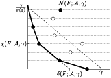
Refer to caption
Figure 3: The critical value and the critical height

6.3 Pre-γ\gamma-final functions

Definition 20.

A γ\gamma-prepared function F∈R𝒜ℓ+1F\in R_{\mathcal{A}}^{\ell+1} is pre-γ\gamma-final if

δ⁡(F,𝒜,γ)=γ\delta(F;\mathcal{A},\gamma)=\gamma

or

δ⁡(F,𝒜,γ)<γandχ⁡(F,𝒜,γ)=0.\delta(F;\mathcal{A},\gamma)<\gamma\quad\text{and}\quad\chi(F;\mathcal{A},\gamma)=0\ .

Pre-γ\gamma-final functions are easily recognizable by its Truncated Newton Polygon as it is represented in Figure 4

Refer to caption
Figure 4: The two pre-γ\gamma-final situations

Let Ψℓ+1\Psi_{\ell+1} be the (ℓ+1)(\ell+1)-nested transformation given in Lemma 8.

Proposition 8.

Let F∈R𝒜ℓ+1F\in R_{\mathcal{A}}^{\ell+1} be a pre-γ\gamma-final function. Consider the (ℓ+1)(\ell+1)-nested transformation

𝒜\textstyle{\mathcal{A}\ignorespaces\ignorespaces\ignorespaces\ignorespaces}π\scriptstyle{\pi}ℬ\textstyle{\mathcal{B}\ignorespaces\ignorespaces\ignorespaces\ignorespaces}Ψℓ+1\scriptstyle{\Psi_{\ell+1}}𝒞\textstyle{\mathcal{C}}

where π:𝒜→ℬ\pi:\mathcal{A}\rightarrow\mathcal{B} is a (ℓ+1)(\ell+1)-Puiseux’s package. Then FF is γ\gamma-final in 𝒞\mathcal{C}.

Proof.

First, suppose we have δ=γ\delta=\gamma. In this situation for each index k≥0k\geq 0 we have

ν𝒜​(Fk)≥γ−k​ν​(z).\nu_{\mathcal{A}}(F_{k})\geq\gamma-k\nu(z)\ .

Let 𝒙′\boldsymbol{x}^{\prime} and z′z^{\prime} be the variables in the parameterized regular local model ℬ\mathcal{B} obtained after perform the (ℓ+1)(\ell+1)-Puiseux’s package. From Equations (4) we know that

z=𝒙′𝜶0​(z′+ξ)β0,with​ν​(𝒙′𝜶0)=ν⁡(z),z=\boldsymbol{x}^{\prime\boldsymbol{\alpha}_{0}}(z^{\prime}+\xi)^{\beta_{0}}\ ,\quad\text{with}\ \nu(\boldsymbol{x}^{\prime\boldsymbol{\alpha}_{0}})=\nu(z)\ ,

hence

νℬ​(zk)=νℬ​(𝒙′k​𝜶0​(z′+ξ)k​β0)=k​ν​(z).\nu_{\mathcal{B}}(z^{k})=\nu_{\mathcal{B}}\left(\boldsymbol{x}^{\prime k\boldsymbol{\alpha}_{0}}(z^{\prime}+\xi)^{k\beta_{0}}\right)=k\nu(z)\ .

Therefore, for each k≥0k\geq 0 we have

νℬ​(zk​Fk)=νℬ​(zk)+νℬ​(Fk)≥γ.\nu_{\mathcal{B}}(z^{k}F_{k})=\nu_{\mathcal{B}}(z^{k})+\nu_{\mathcal{B}}(F_{k})\geq\gamma\ .

It follows that

νℬ​(F)≥γ.\nu_{\mathcal{B}}(F)\geq\gamma\ .

If νℬ​(F)>γ\nu_{\mathcal{B}}(F)>\gamma then FF is γ\gamma-final recessive in ℬ\mathcal{B}, so the same holds in 𝒞\mathcal{C} (Lemma 5). On the other hand, if νℬ​(F)=γ\nu_{\mathcal{B}}(F)=\gamma, then FF is γ\gamma-final (dominant or recessive) in 𝒞\mathcal{C} (see Lemma 8).

Now, suppose δ<γ\delta<\gamma and χ=0\chi=0. In this situation for each index k≥1k\geq 1 we have

ν𝒜​(Fk)>δ−k​ν​(z),\nu_{\mathcal{A}}(F_{k})>\delta-k\nu(z)\ ,

hence

νℬ​(zk​Fk)>δ.\nu_{\mathcal{B}}(z^{k}F_{k})>\delta\ .

As a consequence we have that

νℬ​(F−F0)=νℬ​(F−∑k≥1Fk)>δ,\nu_{\mathcal{B}}(F-F_{0})=\nu_{\mathcal{B}}(F-\sum_{k\geq 1}F_{k})>\delta\ ,

and therefore

ν𝒞​(F−F0)>δ.\nu_{\mathcal{C}}(F-F_{0})>\delta\ .

On the other hand we have that F0F_{0} is dominant in 𝒜\mathcal{A} with explicit value δ\delta, hence

νℬ​(F0)=ν𝒜​(F0)=δ.\nu_{\mathcal{B}}(F_{0})=\nu_{\mathcal{A}}(F_{0})=\delta\ .

By Lemma 8 we know that F0F_{0} is γ\gamma-final dominant in 𝒞\mathcal{C} with value δ\delta. These facts imply that FF is also γ\gamma-final dominant in 𝒞\mathcal{C} with value δ\delta (note that F=F0+(F−F0)F=F_{0}+(F-F_{0})). ∎

6.4 Getting γ\gamma-final functions

In this section we will complete the proof of T4​(ℓ+1)T_{4}(\ell+1) by reductio ad absurdum: we suppose that we have a function F∈R𝒜ℓ+1F\in R_{\mathcal{A}}^{\ell+1} such that there is no (ℓ+1)(\ell+1)-nested transformation 𝒜→ℬ\mathcal{A}\rightarrow\mathcal{B} such that FF is pre-γ\gamma-final in ℬ\mathcal{B} and we will get a contradiction.

Let 𝒜\mathcal{A} be a parameterized regular local model and let F∈R𝒜ℓ+1F\in R_{\mathcal{A}}^{\ell+1} be a function. Assume

  1. 1.

    FF is γ\gamma-prepared;

  2. 2.

    for any (ℓ+1)(\ell+1)-nested transformation 𝒜→ℬ\mathcal{A}\rightarrow\mathcal{B} we have that FF is not pre γ\gamma-final in ℬ\mathcal{B}.

For each index k≥0k\geq 0 let us write

Fk=𝒙𝒒k​F~k+F¯k,ν𝒜​(F¯k)>ν⁡(𝒙𝒒k),F_{k}=\boldsymbol{x}^{\boldsymbol{q}_{k}}\tilde{F}_{k}+\bar{F}_{k}\ ,\quad\nu_{\mathcal{A}}(\bar{F}_{k})>\nu(\boldsymbol{x}^{\boldsymbol{q}_{k}})\ ,

where we require F~k∈k⁡[[y1,y2,…,yℓ]]\tilde{F}_{k}\in k[[y_{1},y_{2},\dots,y_{\ell}]]. We have

ν𝒜​(Fχ)=ν⁡(𝒙𝒒χ)=δ−χ​ν​(z).\nu_{\mathcal{A}}(F_{\chi})=\nu(\boldsymbol{x}^{\boldsymbol{q}_{\chi}})=\delta-\chi\nu(z)\ .

Let ϕ∈K\phi\in K be the (ℓ+1)(\ell+1)-contact rational function ϕℓ+1=zd/𝒙𝒑\phi_{\ell+1}=z^{d}/\boldsymbol{x^{p}}, where dd is the ramification index d⁡(z,𝒜)d(z;\mathcal{A}) (see Section 3.2.3).

Now, consider a level FkF_{k} which gives a point in the critical segment. We have that

ν𝒜​(Fk)=ν⁡(𝒙𝒒k)=δ−k​ν​(z)=ν⁡(𝒙𝒒χ)+(χ−k)​ν​(z).\nu_{\mathcal{A}}(F_{k})=\nu(\boldsymbol{x}^{\boldsymbol{q}_{k}})=\delta-k\nu(z)=\nu(\boldsymbol{x}^{\boldsymbol{q}_{\chi}})+(\chi-k)\nu(z)\ .

Therefore, the index kk must be of the form k=χ−t​dk=\chi-td for some integer 0≤t≤χ/d0\leq t\leq\chi/d. Following Remark 7, we have that

𝒙𝒒χ−t​d=𝒙𝒒χ+t​𝒑\boldsymbol{x}^{\boldsymbol{q}_{\chi-td}}=\boldsymbol{x}^{\boldsymbol{q}_{\chi}+t\boldsymbol{p}}

hence

zχ−t​d​F~χ−t​d=𝒙𝒒χ​zχ​ϕ−t​F~χ−t​d.z^{\chi-td}\tilde{F}_{\chi-td}=\boldsymbol{x}^{\boldsymbol{q}_{\chi}}z^{\chi}\phi^{-t}\tilde{F}_{\chi-td}\ .

Denote by MM the integer part of χ/d\chi/d. For 0≤t≤M0\leq t\leq M define the functions Gt∈k⁡[[y1,y2,…,yℓ]]G_{t}\in k[[y_{1},y_{2},\dots,y_{\ell}]] given by

Gt={F~χ−t​dif ​Fχ−t​d​ gives a point in the critical segment;0otherwise.G_{t}=\left\{\begin{array}[]{ll}\tilde{F}_{\chi-td}&\text{if }F_{\chi-td}\text{ gives a point in the critical segment};\\ 0&\text{otherwise}\ .\end{array}\right.

Note that if Gt≠0G_{t}\neq 0 then it is a unit. For t=0,1,…,Mt=0,1,\dots,M write

Gt=G~t+G¯t,G~t∈k,G¯t∈𝔪​k​[[y1,y2,…,yℓ]].G_{t}=\tilde{G}_{t}+\bar{G}_{t}\ ,\quad\tilde{G}_{t}\in k\ ,\bar{G}_{t}\in\mathfrak{m}k[[y_{1},y_{2},\dots,y_{\ell}]]\ .

Let F~crit\tilde{F}_{\text{crit}} and F¯crit\bar{F}_{\text{crit}} be the functions given by

F~crit:=𝒙𝒒χ​zχ​∑t=0Mϕ−t​G~tandF¯crit:=𝒙𝒒χ​zχ​∑t=0Mϕ−t​G¯t.\tilde{F}_{\text{crit}}:=\boldsymbol{x}^{\boldsymbol{q}_{\chi}}z^{\chi}\sum_{t=0}^{M}\phi^{-t}\tilde{G}_{t}\quad\text{and}\quad\bar{F}_{\text{crit}}:=\boldsymbol{x}^{\boldsymbol{q}_{\chi}}z^{\chi}\sum_{t=0}^{M}\phi^{-t}\bar{G}_{t}\ .

Note that we have

F¯crit∈(y1,y2,…,yℓ)​R𝒜ℓ+1.\bar{F}_{\text{crit}}\in(y_{1},y_{2},\dots,y_{\ell})R_{\mathcal{A}}^{\ell+1}\ . (12)

Denote by F˘\breve{F} the function

F˘:=F−F~crit−F¯crit.\breve{F}:=F-\tilde{F}_{\text{crit}}-\bar{F}_{\text{crit}}\ .

Now we will study the behavior of FF after performing a (ℓ+1)(\ell+1)-nested transformation of the kind

𝒜\textstyle{\mathcal{A}\ignorespaces\ignorespaces\ignorespaces\ignorespaces}π\scriptstyle{\pi}ℬ~\textstyle{\tilde{\mathcal{B}}\ignorespaces\ignorespaces\ignorespaces\ignorespaces}τ\scriptstyle{\tau}ℬ\textstyle{\mathcal{B}}

where π:𝒜→ℬ~\pi:\mathcal{A}\rightarrow\tilde{\mathcal{B}} is a (ℓ+1)(\ell+1)-Puiseux’s package and τ:ℬ~→ℬ\tau:\tilde{\mathcal{B}}\rightarrow\mathcal{B} is a γ\gamma-preparation.

Perform a (ℓ+1)(\ell+1)-Puiseux’s package 𝒜→ℬ~\mathcal{A}\rightarrow\tilde{\mathcal{B}} and let (𝒙~,𝒚~,z~)(\tilde{\boldsymbol{x}},\tilde{\boldsymbol{y}},\tilde{z}) be the coordinates in the parameterized regular local model ℬ~\tilde{\mathcal{B}}. We have

F~crit=𝒙~𝒓​ϕe​∑t=0Mϕ−t​G~tandF¯crit=𝒙~𝒓​ϕe​∑t=0Mϕ−t​G¯t,\tilde{F}_{\text{crit}}=\tilde{\boldsymbol{x}}^{\boldsymbol{r}}\phi^{e}\sum_{t=0}^{M}\phi^{-t}\tilde{G}_{t}\quad\text{and}\quad\bar{F}_{\text{crit}}=\tilde{\boldsymbol{x}}^{\boldsymbol{r}}\phi^{e}\sum_{t=0}^{M}\phi^{-t}\bar{G}_{t}\ ,

where ν⁡(𝒙~𝒓)=δ\nu(\tilde{\boldsymbol{x}}^{\boldsymbol{r}})=\delta. The exponents 𝒓∈ℤ≥0r\boldsymbol{r}\in\mathbb{Z}_{\geq 0}^{r} and e∈ℤ>0e\in\mathbb{Z}_{>0} can be determined using the equalities given in (4). Recall that ϕ=z~+ξ\phi=\tilde{z}+\xi is a unit in Rℬ~ℓ+1R_{\tilde{\mathcal{B}}}^{\ell+1}. We can rewrite the above expressions as

F~crit=𝒙~𝒓​U​∑t=0M(z~+ξ)M−t​G~tandF¯crit=𝒙~𝒓​U​∑t=0M(z~+ξ)M−t​G¯t,\tilde{F}_{\text{crit}}=\tilde{\boldsymbol{x}}^{\boldsymbol{r}}U\sum_{t=0}^{M}(\tilde{z}+\xi)^{M-t}\tilde{G}_{t}\quad\text{and}\quad\bar{F}_{\text{crit}}=\tilde{\boldsymbol{x}}^{\boldsymbol{r}}U\sum_{t=0}^{M}(\tilde{z}+\xi)^{M-t}\bar{G}_{t}\ ,

where U=ϕe−MU=\phi^{e-M} is a unit. Note that we have

νℬ~​(F~crit)=νℬ~​(F¯crit)=δ.\nu_{\tilde{\mathcal{B}}}(\tilde{F}_{\text{crit}})=\nu_{\tilde{\mathcal{B}}}(\bar{F}_{\text{crit}})=\delta\ . (13)

On the other hand, it follows by construction that

νℬ~​(F˘)>δ.\nu_{\tilde{\mathcal{B}}}(\breve{F})>\delta\ . (14)

Note that Equation (12) gives

F¯crit∈(y~1,y~2,…,y~ℓ)​R𝒜~ℓ+1.\bar{F}_{\text{crit}}\in(\tilde{y}_{1},\tilde{y}_{2},\dots,\tilde{y}_{\ell})R_{\tilde{\mathcal{A}}}^{\ell+1}\ . (15)

Let Q∈k⁡[z~]Q\in k[\tilde{z}] be the polynomial

Q=∑t=0MG~t​(z~+ξ)M−t,Q=\sum_{t=0}^{M}\tilde{G}_{t}(\tilde{z}+\xi)^{M-t}\ ,

and denote by ℏ\hbar its order. Note that ℏ≤M≤χ\hbar\leq M\leq\chi and

ℏ=M\displaystyle\hbar=M ⟺\displaystyle\Longleftrightarrow Q=G~0​z~M\displaystyle Q=\tilde{G}_{0}\tilde{z}^{M} (16)
⟺\displaystyle\Longleftrightarrow G~t=(−1)t​ξt​(χt)​μ0for ​1≤t≤M.\displaystyle\tilde{G}_{t}=(-1)^{t}\xi^{t}\binom{\chi}{t}\mu_{0}\quad\text{for }1\leq t\leq M\ .

From Equations (13), (14) and (12) we have that the ℏ\hbar-level of FF in ℬ~\tilde{\mathcal{B}} is dominant.

Now, perform a γ\gamma-preparation ℬ~→ℬ\tilde{\mathcal{B}}\rightarrow\mathcal{B}. Let δ′\delta^{\prime} be the critical value of FF in ℬ\mathcal{B}. By assumption we have δ′<γ\delta^{\prime}<\gamma. Let χ′\chi^{\prime} be the new critical height.

Since the ℏ\hbar-level of FF in ℬ~\tilde{\mathcal{B}} is dominant, the same happens in ℬ\mathcal{B} (Lemma 5). We also have that

νℬ​(F)=νℬ~​(F)=νℬ~​(F~crit+F¯crit+F˘)=δ.\nu_{\mathcal{B}}(F)=\nu_{\tilde{\mathcal{B}}}(F)=\nu_{\tilde{\mathcal{B}}}(\tilde{F}_{\text{crit}}+\bar{F}_{\text{crit}}+\breve{F})=\delta\ .

We conclude that

χ′≤ℏ≤M=[χd]≤χ.\chi^{\prime}\leq\hbar\leq M=\left[\frac{\chi}{d}\right]\leq\chi\ . (17)

Inequality (17) gives

χ′<χ\chi^{\prime}<\chi

except in the case when d=1d=1 and the condition about the coefficients of F~crit\tilde{F}_{\text{crit}} given in (16) is satisfied. Note that we have

χ=χ′⟹νℬ​(F)=δ=δ′−χ​ν​(z′),\chi=\chi^{\prime}\Longrightarrow\nu_{\mathcal{B}}(F)=\delta=\delta^{\prime}-\chi\nu(z^{\prime})\ , (18)

where z′z^{\prime} is the (ℓ+1)(\ell+1)-th dependent variable in ℬ\mathcal{B}.

Suppose that χ′=χ\chi^{\prime}=\chi. In this situation instead of performing the (ℓ+1)(\ell+1)-nested transformation

𝒜\textstyle{\mathcal{A}\ignorespaces\ignorespaces\ignorespaces\ignorespaces}π\scriptstyle{\pi}ℬ~\textstyle{\tilde{\mathcal{B}}\ignorespaces\ignorespaces\ignorespaces\ignorespaces}τ\scriptstyle{\tau}ℬ\textstyle{\mathcal{B}}

we will make an ordered change of the variable zz.

So we have a parameterized regular local model 𝒜\mathcal{A} with d=d⁡(z,𝒜)=1d=d(z;\mathcal{A})=1 and a function F∈R𝒜ℓ+1F\in R_{\mathcal{A}}^{\ell+1} with critical height χ\chi and such that the coefficients of F~crit\tilde{F}_{\text{crit}} satisfy the condition given in (16). Furthermore, following Equation (18), after performing a (ℓ+1)(\ell+1)-Puiseux’s package and a γ\gamma-preparation if necessary, we can assume that

ν𝒜​(F)=ν𝒜​(Fχ).\nu_{\mathcal{A}}(F)=\nu_{\mathcal{A}}(F_{\chi})\ .

Moreover, after performing a 00-nested transformation given by Lemma 4 if necessary, we can suppose that FχF_{\chi} divides FF. So, after factoring FχF_{\chi}, we can assume that

ν𝒜​(F)=ν𝒜​(Fχ)=1andFχ=1.\nu_{\mathcal{A}}(F)=\nu_{\mathcal{A}}(F_{\chi})=1\quad\text{and}\quad F_{\chi}=1\ .

Since FF is γ\gamma-prepared, the level at height (χ−1)(\chi-1) has the form

Fχ−1=𝒙𝒑​F~χ−1+F¯χ−1,ν𝒜​(F¯χ−1)>ν⁡(𝒙𝒑),F_{\chi-1}=\boldsymbol{x}^{\boldsymbol{p}}\tilde{F}_{\chi-1}+\bar{F}_{\chi-1}\ ,\quad\nu_{\mathcal{A}}(\bar{F}_{\chi-1})>\nu(\boldsymbol{x}^{\boldsymbol{p}})\ ,

where F~χ−1\tilde{F}_{\chi-1} is a unit which does not depend on the independent variables 𝒙\boldsymbol{x}. Let us write F~χ−1\tilde{F}_{\chi-1} as a power series

F~χ−1=∑(I,J)∈ℤ≥0r+ℓfI​J​𝒙I​𝒚J,fI​J∈k.\tilde{F}_{\chi-1}=\sum_{(I,J)\in\mathbb{Z}^{r+\ell}_{\geq 0}}f_{IJ}\boldsymbol{x}^{I}\boldsymbol{y}^{J}\ ,\quad f_{IJ}\in k\ .

Denote

F~χ−1=G+H\tilde{F}_{\chi-1}=G+H

where G∈k⁡[𝒙,𝒚]⊂R𝒜ℓG\in k[\boldsymbol{x},\boldsymbol{y}]\subset R_{\mathcal{A}}^{\ell} is the polynomial

G=∑(I,J)∈ℤ≥0r+ℓν⁡(𝒙I​𝒚J)≤2​ν​(z)fI​J​𝒙I​𝒚J.G=\sum_{\begin{subarray}{c}(I,J)\in\mathbb{Z}^{r+\ell}_{\geq 0}\\ \nu(\boldsymbol{x}^{I}\boldsymbol{y}^{J})\leq 2\nu(z)\end{subarray}}f_{IJ}\boldsymbol{x}^{I}\boldsymbol{y}^{J}\ \ .

Since the coefficients of FF satisfy the conditions given in (16) we have

G=−ξ​χ​𝒙𝒑+⋯.G=-\xi\chi\boldsymbol{x}^{\boldsymbol{p}}+\cdots\ .

Note that

ν𝒜​(F~χ−1)=ν𝒜​(G)=ν⁡(z)≤ν𝒜​(H).\nu_{\mathcal{A}}(\tilde{F}_{\chi-1})=\nu_{\mathcal{A}}(G)=\nu(z)\leq\nu_{\mathcal{A}}(H)\ . (19)

Now consider the ordered change of coordinates

z~=z−ϕ,whereϕ:=−1χ​G,\tilde{z}=z-\phi\ ,\quad\text{where}\quad\phi:=\frac{-1}{\chi}G\ ,

and let 𝒜~\tilde{\mathcal{A}} be the parameterized regular local model obtained. Note that

ν⁡(z~)≥ν⁡(z).\nu(\tilde{z})\geq\nu(z)\ .

We have

F=∑k=0∞zk​Fk=∑k=0∞(z~+ϕ)k​Fk=∑k=0∞z~k​Fk′,F=\sum_{k=0}^{\infty}z^{k}F_{k}=\sum_{k=0}^{\infty}\left(\tilde{z}+\phi\right)^{k}F_{k}=\sum_{k=0}^{\infty}\tilde{z}^{k}F^{\prime}_{k}\ ,

where

Fk′=Fk+∑i=1∞(k+ii)​ϕi​Fk+i.F^{\prime}_{k}=F_{k}+\sum_{i=1}^{\infty}\binom{k+i}{i}\phi^{i}F_{k+i}\ .

So the (χ−1)(\chi-1)-level of FF in 𝒜~\tilde{\mathcal{A}} is

Fχ−1′=Fχ−1+χ​ϕ​Fχ+ϕ2​(⋯)=G+H−G+ϕ2​(⋯)=H+ϕ2​(⋯).F^{\prime}_{\chi-1}=F_{\chi-1}+\chi\phi F_{\chi}+\phi^{2}(\cdots)=G+H-G+\phi^{2}(\cdots)=H+\phi^{2}(\cdots)\ . (20)

In 𝒜~\tilde{\mathcal{A}} the function FF is not necessarily γ\gamma-prepared so let 𝒜~→𝒜1\tilde{\mathcal{A}}\rightarrow\mathcal{A}_{1} a γ\gamma-preparation.

It follows from the definition of HH and Equations (19) and (20) that

ν𝒜1​(Fχ−1′)≥2​ν​(z).\nu_{\mathcal{A}_{1}}(F^{\prime}_{\chi-1})\geq 2\nu(z)\ .

Note also that we still have

ν𝒜1​(F)=ν𝒜1​(Fχ′)=0.\nu_{\mathcal{A}_{1}}(F)=\nu_{\mathcal{A}_{1}}(F^{\prime}_{\chi})=0\ .

Let z1z_{1} be the (ℓ+1)(\ell+1)-th dependent variable in 𝒜1\mathcal{A}_{1}. We have that

χ⁡(F,𝒜1,γ)≤χ⁡(F,𝒜,γ).\chi(F;\mathcal{A}_{1},\gamma)\leq\chi(F;\mathcal{A},\gamma)\ .

Furthermore, we have

χ⁡(F,𝒜1,γ)=χ⁡(F,𝒜,γ)⟹ν⁡(z1)=ν𝒜1​(Fχ−1′)≥2​ν​(z).\chi(F;\mathcal{A}_{1},\gamma)=\chi(F;\mathcal{A},\gamma)\Longrightarrow\nu(z_{1})=\nu_{\mathcal{A}_{1}}(F^{\prime}_{\chi-1})\geq 2\nu(z)\ . (21)

Now, we can perform a z1z_{1}-Puiseux’s package. If the critical height does not drop, instead of performing a z1z_{1}-Puiseux’s package we make an ordered change of coordinates as above. We iterate this procedure while the critical height does not drop. At each step we obtain a parameterized regular local model 𝒜i\mathcal{A}_{i}. By Equation (21) we know that the (ℓ+1)(\ell+1)-th dependent variable ziz_{i} satisfies

ν⁡(zi)≥2i​ν​(z).\nu(z_{i})\geq 2^{i}\nu(z)\ .

This can not happen infinitely many times, since in a finite number of steps we reach a parameterized regular local model 𝒜i0\mathcal{A}_{i_{0}} such that

ν⁡(zi0)≥γ−ν𝒜​(F)χ=γ−ν𝒜i0​(F)χ.\nu(z_{i_{0}})\geq\frac{\gamma-\nu_{\mathcal{A}}(F)}{\chi}=\frac{\gamma-\nu_{\mathcal{A}_{i_{0}}}(F)}{\chi}\ .

The above inequality implies that δ⁡(F,𝒜i0,γ)=γ\delta(F;\mathcal{A}_{i_{0}},\gamma)=\gamma which is in contradiction with our assumptions.

Then, after a finite number of ordered changes of the (ℓ+1)(\ell+1)-th variable and γ\gamma-preparations of FF, necessarily we reach a parameterized regular local model in which the critical height drops by means of a (ℓ+1)(\ell+1)-Puiseux’s package. Again, this can not happen infinitely many times since we are assuming that the critical height is strictly positive.

We have just proved that our assumptions give a contradiction, so there is always a (ℓ+1)(\ell+1)-nested transformation which transform a function into a γ\gamma-final one. Thus, we have prove that

T4​(ℓ)⟹T4​(ℓ+1).T_{4}(\ell)\Longrightarrow T_{4}(\ell+1)\ .

7 Truncated preparation of a 11-form

In this chapter and the next one we will detail the proof of

T3​(ℓ)⟹T3​(ℓ+1).T_{3}(\ell)\Longrightarrow T_{3}(\ell+1)\ .

We will adapt the arguments used in Chapter 6 to the case of 11-forms. As the name of the chapter says, this chapter is the equivalent for 11-forms of the Section 6.1.

Let 𝒜=(𝒪,(𝒙,𝒚))\mathcal{A}=\big(\mathcal{O},(\boldsymbol{x},\boldsymbol{y})\big) be a parameterized regular local model of K,νK,\nu. Fix an index ℓ\ell, 0≤ℓ≤n−r−10\leq\ell\leq n-r-1 and a value γ∈Γ\gamma\in\Gamma. We consider a 1-form ω∈N𝒜l+1\omega\in N_{\mathcal{A}}^{l+1} such that ν𝒜​(ω∧d​ω)≥2​γ\nu_{\mathcal{A}}(\omega\wedge d\omega)\geq 2\gamma. Since we are working by induction on ℓ\ell, we assume that the statement T3​(ℓ)T_{3}(\ell) is true (hence T4​(ℓ)T_{4}(\ell) and T5​(ℓ)T_{5}(\ell) are also true).

7.1 Expansions relative to a dependent variable

Let us denote the dependent variable yl+1y_{l+1} by zz. Note that by definition

R𝒜l+1=R𝒜ℓ​[[z]].R_{\mathcal{A}}^{l+1}=R_{\mathcal{A}}^{\ell}[[z]]\ .

Thus we can expand an element F∈R𝒜l+1F\in R_{\mathcal{A}}^{l+1} as a power series in the variable zz:

F=∑k=0∞Fk​zk,Fk∈R𝒜ℓ.F=\sum_{k=0}^{\infty}F_{k}z^{k}\quad,\ F_{k}\in R_{\mathcal{A}}^{\ell}.

Take an element of N𝒜l+1N_{\mathcal{A}}^{l+1}

ω=∑i=1rai​d​xixi+∑j=1ℓbj​d​yj+c​d​z.\omega=\sum_{i=1}^{r}a_{i}\frac{dx_{i}}{x_{i}}+\sum_{j=1}^{\ell}b_{j}dy_{j}+cdz\ .

Write

ω=∑i=1rai​d​xixi+∑j=1ℓbj​d​yj+f​d​zz,\omega=\sum_{i=1}^{r}a_{i}\frac{dx_{i}}{x_{i}}+\sum_{j=1}^{\ell}b_{j}dy_{j}+f\frac{dz}{z}\ ,

where f=z​cf=zc. The decomposition in zz-levels of ω\omega of consists in writing ω\omega as

ω=∑k=0∞zk​ωk=∑k=0∞zk​(∑i=1rai​k​d​xixi+∑j=1ℓbj​k​d​yj+fk​d​zz).\omega=\sum_{k=0}^{\infty}z^{k}\omega_{k}=\sum_{k=0}^{\infty}z^{k}\Big(\sum_{i=1}^{r}a_{ik}\frac{dx_{i}}{x_{i}}+\sum_{j=1}^{\ell}b_{jk}dy_{j}+f_{k}\frac{dz}{z}\Big)\ . (22)

where

ai=∑k=0∞ai​k​zk,bj=∑k=0∞bj​k​zk​ and ​f=∑k=1∞f0​zk.a_{i}=\sum_{k=0}^{\infty}a_{ik}z^{k}\ ,\ b_{j}=\sum_{k=0}^{\infty}b_{jk}z^{k}\ \text{ and }\ f=\sum_{k=1}^{\infty}f_{0}z^{k}\ .

Note that f0=0f_{0}=0. We say that ωk\omega_{k} is the kk-level of ω\omega.

Remark 18.

The coefficients of each zz-level ωk\omega_{k} are elements of R𝒜ℓR_{\mathcal{A}}^{\ell}, but ωk\omega_{k} itself belongs neither to N𝒜ℓN_{\mathcal{A}}^{\ell} nor to N𝒜l+1N_{\mathcal{A}}^{l+1}. The zz-levels ωk\omega_{k} belong to the R𝒜ℓR_{\mathcal{A}}^{\ell}-module N𝒜ℓ⊕R𝒜ℓ​d​zzN_{\mathcal{A}}^{\ell}\oplus R_{\mathcal{A}}^{\ell}\frac{dz}{z}. We will write

ωk=ηk+fk​d​zz∈N𝒜ℓ⊕R𝒜ℓ​d​zz,∀k≥0,\omega_{k}=\eta_{k}+f_{k}\frac{dz}{z}\in N_{\mathcal{A}}^{\ell}\oplus R_{\mathcal{A}}^{\ell}\frac{dz}{z}\ ,\ \forall k\geq 0\ ,

where we denote by ηk∈N𝒜ℓ\eta_{k}\in N_{\mathcal{A}}^{\ell} the 11-forms

ηk:=∑i=1rai​k​d​xixi+∑j=1ℓbj​k​d​yj,∀k≥0.\eta_{k}:=\sum_{i=1}^{r}a_{ik}\frac{dx_{i}}{x_{i}}+\sum_{j=1}^{\ell}b_{jk}dy_{j}\ ,\ \forall k\geq 0\ .

To each level we can attach a pair

ωk=ηk+fk​d​zz⟼(ηk,fk)∈N𝒜ℓ×R𝒜ℓ.\omega_{k}=\eta_{k}+f_{k}\frac{dz}{z}\longmapsto(\eta_{k},f_{k})\in N_{\mathcal{A}}^{\ell}\times R_{\mathcal{A}}^{\ell}\ .

Denote by δk​(ω,𝒜),ϕk​(ω,𝒜),βk​(ω,𝒜)∈Γ∪{∞}\delta_{k}(\omega;\mathcal{A}),\phi_{k}(\omega;\mathcal{A}),\beta_{k}(\omega;\mathcal{A})\in\Gamma\cup\{\infty\} the explicit values

δk​(ω,𝒜)\displaystyle\delta_{k}(\omega;\mathcal{A}) :⁣=\displaystyle:= ν𝒜​(ηk),\displaystyle\nu_{\mathcal{A}}(\eta_{k})\ ,
ϕk​(ω,𝒜)\displaystyle\phi_{k}(\omega;\mathcal{A}) :⁣=\displaystyle:= ν𝒜​(fk),\displaystyle\nu_{\mathcal{A}}(f_{k})\ ,
βk​(ω,𝒜)\displaystyle\beta_{k}(\omega;\mathcal{A}) :⁣=\displaystyle:= ν𝒜​(ηk,fk)=min⁡{ϕk​(ω,𝒜),ηk​(ω,𝒜)}.\displaystyle\nu_{\mathcal{A}}(\eta_{k},f_{k})=\min\left\{\phi_{k}(\omega;\mathcal{A}),\eta_{k}(\omega;\mathcal{A})\right\}\ .

The value βk​(ω,𝒜)\beta_{k}(\omega;\mathcal{A}) is the explicit value of ωk\omega_{k}. If no confusion arises we denote δk​(ω,𝒜)\delta_{k}(\omega;\mathcal{A}), ϕk​(ω,𝒜)\phi_{k}(\omega;\mathcal{A}) and βk​(ω,𝒜)\beta_{k}(\omega;\mathcal{A}) by δk\delta_{k}, ϕk\phi_{k} and βk\beta_{k} respectively. Given α∈Γ\alpha\in\Gamma we say that the level ωk\omega_{k} is α\alpha-final (final dominant, final recessive) if and only if the pair (ηk,fk)(\eta_{k},f_{k}) is α\alpha-final (final dominant, final recessive). In particular, we say that a level ωk\omega_{k} is log-elementary if it is 00-final dominant, and that it is dominant if it is βk\beta_{k}-final dominant.

From Lemmas 5, 6 and 7 we obtain the following property of stability of δk\delta_{k}, ϕk\phi_{k} and βk\beta_{k} under any ℓ\ell-nested transformation:

Property of stability of levels. For any ℓ\ell-nested transformation 𝒜→𝒜′{\mathcal{A}}\rightarrow{\mathcal{A}}^{\prime} and any k≥0k\geq 0, we have that δk′≥δk\delta_{k}^{\prime}\geq\delta_{k}, ϕk′≥ϕk\phi_{k}^{\prime}\geq\phi_{k} and βk′≥βk\beta_{k}^{\prime}\geq\beta_{k}.

In addition we have stability for dominant levels:

Property of stability for dominant levels. Given a dominant level ωk\omega_{k} and any ℓ\ell-nested transformation 𝒜→𝒜′{\mathcal{A}}\rightarrow{\mathcal{A}}^{\prime}, the transformed level ωk′\omega^{\prime}_{k} is also dominant and βk′=βk\beta_{k}^{\prime}=\beta_{k}.

7.2 Truncated Newton polygons and prepared 11-forms

Using the values defined in the previous section we define certain subsets of Γ≥0×ℤ≥0⊂ℝ≥02\Gamma_{\geq 0}\times\mathbb{Z}_{\geq 0}\subset\mathbb{R}_{\geq 0}^{2}. The Cloud of Points of ω\omega is the discrete subset

CL(ω;𝒜):={(βk,k)|k=0,1,…}.\operatorname{CL}(\omega;\mathcal{A}):=\left\{(\beta_{k},k)\ |\ k=0,1,\dots\right\}\ .

Note that

ω≠0⇒CL⁡(ω;𝒜)≠∅.\omega\neq 0\Rightarrow\operatorname{CL}(\omega;\mathcal{A})\neq\emptyset\ .

We also use the Dominant Cloud of Points of ω\omega

DomCL⁡(ω;𝒜):={(βk,k)∈CL⁡(ω;𝒜)|ωk​ is dominant}.\operatorname{DomCL}(\omega;\mathcal{A}):=\left\{(\beta_{k},k)\in\operatorname{CL}(\omega;\mathcal{A})\ |\ \omega_{k}\text{ is dominant}\right\}\ .

Note that DomCL⁡(ω,𝒜)\operatorname{DomCL}(\omega;\mathcal{A}) can be empty. In Figure 5 we can see an example in which the points (βk,k)(\beta_{k},k) are represented with black and white circles, corresponding to dominant and non-dominant levels respectively.

Refer to caption
Figure 5: The Cloud of Points and the Dominant Cloud of Points

Given a value σ∈Γ\sigma\in\Gamma, we define the truncated polygons

𝒩⁡(ω,𝒜,σ)andDom⁡𝒩⁡(ω,𝒜,σ)\mathcal{N}(\omega;\mathcal{A},\sigma)\quad\text{and}\quad\operatorname{Dom}\mathcal{N}(\omega;\mathcal{A},\sigma)

to be the respective positively convex hulls of

{(0,σ/ν⁡(z)),(σ,0)}∪CL⁡(ω;𝒜)\{(0,\sigma/\nu(z)),(\sigma,0)\}\cup\operatorname{CL}(\omega;\mathcal{A})

and

{(0,σ/ν⁡(z)),(σ,0)}∪DomCL⁡(ω;𝒜).\{(0,\sigma/\nu(z)),(\sigma,0)\}\cup\operatorname{DomCL}(\omega;\mathcal{A})\ .

Note that for any σ∈Γ\sigma\in\Gamma we have that

𝒩⁡(ω,𝒜,σ)⊃Dom⁡𝒩⁡(ω,𝒜,σ).\mathcal{N}(\omega;\mathcal{A},\sigma)\supset\operatorname{Dom}\mathcal{N}(\omega;\mathcal{A},\sigma)\ .

In Figure 6 we can see the truncated polygons corresponding to the cloud of points represented in Figure 5. Note that in this example Dom⁡𝒩⁡(ω,𝒜,γ)\operatorname{Dom}\mathcal{N}(\omega;\mathcal{A},\gamma) has the vertex (0,γ/ν⁡(z))(0,\gamma/\nu(z)) which does not correspond to any level.

Refer to caption
Figure 6: The Truncated Newton Polygon and the Dominant Truncated Newton Polygon

For each k≥0k\geq 0 let us consider the real number

τk​(ω,𝒜,γ):=min⁡{u|(u,k)∈Dom⁡𝒩⁡(ω,𝒜,γ)}.\tau_{k}(\omega;\mathcal{A},\gamma):=\min\{u\ |\ (u,k)\in\operatorname{Dom}\mathcal{N}(\omega;\mathcal{A},\gamma)\}\ .

Note that 0≤τk​(ω,𝒜,γ)≤max⁡{0,γ−k​ν​(z)}0\leq\tau_{k}(\omega;\mathcal{A},\gamma)\leq\max\{0,\gamma-k\nu(z)\}.

Definition 21.

We say that ω\omega is γ\gamma-prepared in 𝒜\mathcal{A} if and only if the level ωk\omega_{k} is τk​(ω,𝒜,γ)\tau_{k}(\omega;\mathcal{A},\gamma)-final for any 0≤k≤γ/ν⁡(z)0\leq k\leq\gamma/\nu(z).

The example represented in Figures 5 and 6 corresponds to a non γ\gamma-prepared 11-form.

Remark 19.

Note that being γ\gamma-prepared implies that 𝒩⁡(ω,𝒜,γ)=Dom​𝒩\mathcal{N}(\omega;\mathcal{A},\gamma)=\operatorname{Dom\mathcal{N}}. Conversely, if we have that 𝒩⁡(ω,𝒜,γ)=Dom​𝒩\mathcal{N}(\omega;\mathcal{A},\gamma)=\operatorname{Dom\mathcal{N}} to assure that ω\omega is γ\gamma-prepared it is enough to guarantee that βk>τk\beta_{k}>\tau_{k} for any level ωk\omega_{k} which is not τk\tau_{k}-dominant. This last condition can be obtained applying Lemma 8.

The objective of this chapter is to prove the following result

Theorem IX (Existence of γ\gamma-preparation).

Let ω∈N𝒜ℓ+1\omega\in N_{\mathcal{A}}^{\ell+1} be a 11-form such that ν𝒜​(ω∧d​ω)≥2​γ\nu_{\mathcal{A}}(\omega\wedge d\omega)\geq 2\gamma. There is a ℓ\ell-nested transformation 𝒜→ℬ\mathcal{A}\rightarrow\mathcal{B} such that ω\omega is γ\gamma-prepared in ℬ\mathcal{B}.

A ℓ\ell-nested transformation 𝒜→ℬ\mathcal{A}\rightarrow\mathcal{B} such that ω\omega is γ\gamma-prepared in ℬ\mathcal{B} is called a γ\gamma-preparation.

7.3 Property of preparation of levels

Consider and integer number k≥0k\geq 0 and put

λk(ω;𝒜,γ)=min{γ−kν(z)}∪{δk+s+δk−s2|s≥1}.\lambda_{k}(\omega;\mathcal{A},\gamma)=\min\{\gamma-k\nu(z)\}\cup\left\{\frac{\delta_{k+s}+\delta_{k-s}}{2}\ |\ \quad s\geq 1\right\}\ . (23)

In this section we prove the following Lemma

Lemma 9.

There is an ℓ\ell-nested transformation 𝒜→𝒜′{\mathcal{A}}\rightarrow{\mathcal{A}}^{\prime} such that the kk-level ωk′\omega^{\prime}_{k} of ω\omega with respect to 𝒜′{\mathcal{A}}^{\prime} is λk​(𝒜,ω,γ)\lambda_{k}({\mathcal{A}};\omega,\gamma)-final.

This result is a consequence of the induction hypothesis and the fact that ν𝒜​(ω∧d​ω)≥2​γ\nu_{\mathcal{A}}(\omega\wedge d\omega)\geq 2\gamma. Namely, we can write

ω∧d​ω=∑m=0∞zm​(Θm+d​zz∧Δm)\omega\wedge d\omega=\sum_{m=0}^{\infty}z^{m}\Big(\Theta_{m}+\frac{dz}{z}\wedge\Delta_{m}\Big)

where

Θm:=∑i+j=mηi∧d​ηj\Theta_{m}:=\sum_{i+j=m}\eta_{i}\wedge d\eta_{j}

and

Δm:=∑i+j=mj​ηj∧ηi+fi​d​ηj+ηi∧d​fj.\Delta_{m}:=\sum_{i+j=m}j\eta_{j}\wedge\eta_{i}+f_{i}d\eta_{j}+\eta_{i}\wedge df_{j}\ .

We have that

ν𝒜​(ω∧d​ω)≥2​γ\nu_{\mathcal{A}}(\omega\wedge d\omega)\geq 2\gamma

is equivalent to

ν𝒜​(Θm)≥2​γ​ and ​ν𝒜​(Δm)≥2​γ∀m≥0.\nu_{\mathcal{A}}(\Theta_{m})\geq 2\gamma\text{ and }\nu_{\mathcal{A}}(\Delta_{m})\geq 2\gamma\quad\forall\,m\geq 0\ .

The proof of Lemma 9 is based on this equivalence. In view of the statement T3​(ℓ)T_{3}(\ell) it is enough to prove that

ν𝒜​(ηk∧d​ηk)≥2​λk.\nu_{\mathcal{A}}(\eta_{k}\wedge d\eta_{k})\geq 2\lambda_{k}\ .

Look at Θ2​k\Theta_{2k}:

Θ2​k=ηk∧d​ηk+∑i+j=2​ki,j≠kηi∧d​ηj.\Theta_{2k}=\eta_{k}\wedge d\eta_{k}+\sum_{\begin{subarray}{c}i+j=2k\\ i,j\neq k\end{subarray}}\eta_{i}\wedge d\eta_{j}\ .

Recall that ν𝒜​(Θ2​k)≥2​γ\nu_{\mathcal{A}}(\Theta_{2k})\geq 2\gamma. By definition of the values δi\delta_{i}, we have that ν𝒜​(ηi)≥δi\nu_{\mathcal{A}}(\eta_{i})\geq\delta_{i}, hence ν𝒜​(d​ηi)≥δi\nu_{\mathcal{A}}(d\eta_{i})\geq\delta_{i}. Writing

ηk∧d​ηk=−Θ2​k+∑i+j=2​ki,j≠kηi∧d​ηj,\eta_{k}\wedge d\eta_{k}=-\Theta_{2k}+\sum_{\begin{subarray}{c}i+j=2k\\ i,j\neq k\end{subarray}}\eta_{i}\wedge d\eta_{j}\ ,

we conclude that ν𝒜​(ηk∧d​ηk)≥2​λk\nu_{\mathcal{A}}(\eta_{k}\wedge d\eta_{k})\geq 2\lambda_{k}. We end the proof of Lemma 9 applying T5​(ℓ)T_{5}(\ell) to the pair (ηk,fk)(\eta_{k},f_{k}).

7.4 Preparation. First reductions

In order to prove Theorem IX we will first show that we can assume some reductions.

Proposition 9.

Let ω∈N𝒜ℓ+1\omega\in N_{\mathcal{A}}^{\ell+1} be a 11-form such that ν𝒜​(ω∧d​ω)≥2​γ\nu_{\mathcal{A}}(\omega\wedge d\omega)\geq 2\gamma. Without lost of generality we can assume that the following properties are satisfied:

  1. 1.

    Maximality of dominant levels: For any integer number kk with 0≤k≤γ/ν⁡(z)0\leq k\leq\gamma/\nu(z), the level ωk\omega_{k} is either (γ−k​ν​(z))(\gamma-k\nu(z))-final dominant in 𝒜\mathcal{A} or there is no ℓ\ell-nested transformation 𝒜→𝒜′\mathcal{A}\rightarrow\mathcal{A}^{\prime} such that ωk\omega_{k} is (γ−k​ν​(z))(\gamma-k\nu(z))-final dominant in 𝒜′\mathcal{A}^{\prime};

  2. 2.

    Preparation of the functional part: For any integer number kk with 0≤k≤γ/ν⁡(z)0\leq k\leq\gamma/\nu(z), the function fk∈R𝒜ℓf_{k}\in R_{\mathcal{A}}^{\ell} is (γ−k​ν​(z))(\gamma-k\nu(z))-final;

  3. 3.

    Preparation of the 00-level: The 00-level ω0\omega_{0} is γ\gamma-final;

  4. 4.

    Explicitness of the dominant vertices: Any vertex of Dom⁡𝒩⁡(ω,𝒜,γ)\operatorname{Dom}\mathcal{N}(\omega;\mathcal{A},\gamma) is also a vertex of 𝒩⁡(ω,𝒜,γ)\mathcal{N}(\omega;\mathcal{A},\gamma).

First of all, note that the four properties listed in the proposition are stable under further ℓ\ell-nested transformations. The first property can be obtained without making use of the induction hypothesis while the remaining ones needs the assumption that T3​(ℓ)T_{3}(\ell) is true. In this section we detail how to obtain the first three properties. The following section is devoted to show how to obtain explicit dominant vertices.

Maximality of dominant levels: This property can be obtained thanks to the stability of dominant levels as follows. Take an integer kk with 0≤k≤γ/ν⁡(z)0\leq k\leq\gamma/\nu(z). If there is a ℓ\ell-nested transformation such that ωk\omega_{k} becomes (γ−k​ν​(z))(\gamma-k\nu(z))-final dominant, perform it. In this way we perform a finite number of transformations to get the desired maximality property.

Preparation of the functional part: We only have to use T4​(ℓ)T_{4}(\ell) finitely many times.

Preparation of the 00-level: This property is also obtained using the induction hypothesis. We have that ν𝒜​(ω∧d​ω)≥2​γ\nu_{\mathcal{A}}(\omega\wedge d\omega)\geq 2\gamma implies ν𝒜​(Θ0)≥2​γ\nu_{\mathcal{A}}(\Theta_{0})\geq 2\gamma. Since Θ0=η0∧d​η0\Theta_{0}=\eta_{0}\wedge d\eta_{0} we can invoke T3​(ℓ)T_{3}(\ell) and transform ω0\omega_{0} into a γ\gamma-final level.

7.5 Getting explicit dominant vertices

In this section we complete the proof of Proposition 9 by showing how to obtain explicit dominant vertices. First of all, note that the maximality of dominant vertices property implies the following additional property:

Stability of the Truncated Dominant Newton Polygon: For any ℓ\ell-nested transformation 𝒜→𝒜′\mathcal{A}\rightarrow\mathcal{A}^{\prime} we have that

Dom​𝒩​(ω,𝒜,γ)=Dom​𝒩​(ω,𝒜′,γ).\textrm{Dom}\mathcal{N}(\omega;\mathcal{A},\gamma)=\textrm{Dom}\mathcal{N}(\omega;\mathcal{A}^{\prime},\gamma)\ .

In view of this stability property, from now on we will denote the Truncated Dominant Newton Polygon Dom​𝒩​(ω,𝒜,γ)\textrm{Dom}\mathcal{N}(\omega;\mathcal{A},\gamma) simply by Dom​𝒩\textrm{Dom}\mathcal{N}, and the values τk​(ω,𝒜,γ)\tau_{k}(\omega;\mathcal{A},\gamma) by τk\tau_{k}.

For any positive real number δ>0\delta>0, let us consider the lines

Lδ​(ρ)={(u,v)|u+δ​v=ρ}L_{\delta}(\rho)=\{(u,v)\ |\ u+\delta v=\rho\}

of slope −1/δ-1/\delta, and the open half-planes

Hδ+​(ρ)={(u,v)|u+δ​v>ρ}andHδ−​(ρ)={(u,v)|u+δ​v<ρ}.H^{+}_{\delta}(\rho)=\{(u,v)\ |\ u+\delta v>\rho\}\quad\text{and}\quad H^{-}_{\delta}(\rho)=\{(u,v)\ |\ u+\delta v<\rho\}\ .

Let ρδ\rho_{\delta} be the real number defined by

ρδ:=min⁡{ρ|Lδ​(ρ)∩Dom⁡𝒩≠∅}=sup{ρ|Hδ+​(ρ)⊃Dom⁡𝒩}.\rho_{\delta}:=\min\{\rho\ |\ L_{\delta}(\rho)\cap\operatorname{Dom}\mathcal{N}\neq\emptyset\}=\sup\{\rho\ |\ H^{+}_{\delta}(\rho)\supset\operatorname{Dom}\mathcal{N}\}\ .

We have that Lδ​(ρδ)L_{\delta}(\rho_{\delta}) cuts the polygon Dom⁡𝒩\operatorname{Dom}\mathcal{N} in only one vertex or a side joining two vertices.

In order to get explicit dominant vertices, it is enough to prove the following lemma:

Lemma 10.

Given δ>0\delta>0 and a fixed ϵ>0\epsilon>0 there is an ℓ\ell-nested transformation 𝒜→𝒜′\mathcal{A}\rightarrow\mathcal{A}^{\prime} such that 𝒩⁡(ω,𝒜′,γ)⊂Hδ+​(ρδ−ϵ)\mathcal{N}(\omega;\mathcal{A}^{\prime},\gamma)\subset H^{+}_{\delta}(\rho_{\delta}-\epsilon).

Note that as usual, the property obtained after applying the lemma is stable under new ℓ\ell-nested transformations.

Let us show that Lemma 10 allows us to get the explicitness of dominant vertices property. Consider a vertex 𝒗=(τk,k)\boldsymbol{v}=(\tau_{k},k) of Dom⁡𝒩\operatorname{Dom}\mathcal{N}. Take two slopes 0<δ2<δ10<\delta_{2}<\delta_{1} such that both Lδ1​(ρδ1)L_{{\delta_{1}}}(\rho_{{\delta}_{1}}) and Lδ2​(ρδ2)L_{{\delta_{2}}}(\rho_{{\delta}_{2}}) cut the polygon Dom⁡𝒩\operatorname{Dom}\mathcal{N} only in the vertex 𝒗\boldsymbol{v}. Consider an slope δ3\delta_{3} with δ2<δ3<δ1\delta_{2}<\delta_{3}<\delta_{1}. We also have that Lδ3​(ρδ3)L_{\delta_{3}}(\rho_{\delta_{3}}) cuts Dom⁡𝒩\operatorname{Dom}\mathcal{N} only in the vertex 𝒗{\boldsymbol{v}}. By an elementary geometrical argument, we see that there is an ϵ>0\epsilon>0 satisfying the following property

“For any (a,k′)∈Hδ1+​(ρδ1−ϵ)∩Hδ2+​(ρδ2−ϵ)(a,k^{\prime})\in H^{+}_{{\delta_{1}}}(\rho_{{\delta}_{1}}-\epsilon)\cap H^{+}_{{\delta_{2}}}(\rho_{{\delta}_{2}}-\epsilon) such that k′≠kk^{\prime}\neq k we have that (a,k′)∈Hδ3+​(ρδ3)(a,k^{\prime})\in H^{+}_{{\delta_{3}}}(\rho_{{\delta}_{3}})”.

Applying Lemma 10 with respect to ϵ\epsilon, we obtain that 𝒗\boldsymbol{v} is a vertex of 𝒩⁡(ω,𝒜′,γ)\mathcal{N}(\omega;\mathcal{A}^{\prime},\gamma). Repeating this argument at all the vertices of Dom⁡𝒩\operatorname{Dom}\mathcal{N} we obtain the explicitness of dominant vertices property.

Refer to caption
Figure 7: Situation after applying Lemma 10

So in order to complete the proof of Proposition 9 we have to prove Lemma 10. Denote by (αk,k)(\alpha_{k},k) the point in 𝒩⁡(ω,𝒜,γ)\mathcal{N}(\omega;\mathcal{A},\gamma) with integer ordinate equal to kk and smallest abscissa. Note that

αk≤τk.\alpha_{k}\leq\tau_{k}\ .

Note also that α0≤γ\alpha_{0}\leq\gamma and αk=0\alpha_{k}=0 for any k>γ/ν⁡(z)k>\gamma/\nu(z). We use as a key argument the following property

Reduction of vertices: Consider a vertex 𝒗=(αk,k)\boldsymbol{v}=(\alpha_{k},k) of the polygon 𝒩⁡(ω,𝒜,γ)\mathcal{N}(\omega;\mathcal{A},\gamma) which is not a vertex of Dom⁡𝒩\operatorname{Dom}\mathcal{N} (in particular k≥1k\geq 1). There is a ℓ\ell-nested transformation 𝒜→𝒜\mathcal{A}\rightarrow\mathcal{A} such that

𝒩⁡(ω,𝒜′,λ)⊂𝒩′\mathcal{N}(\omega;\mathcal{A}^{\prime},\lambda)\subset\mathcal{N}^{\prime}

where 𝒩′\mathcal{N}^{\prime} is the positively convex polygon generated by {(αs′,s)}s≥0\{(\alpha^{\prime}_{s},s)\}_{s\geq 0} where

αs′={αs, if ​s≠k;αk−1+αk+12, if ​s=k.\alpha^{\prime}_{s}=\left\{\begin{array}[]{lc}\alpha_{s}\ ,&\text{ if }s\neq k\ ;\\ \frac{\alpha_{k-1}+\alpha_{k+1}}{2}\ ,&\text{ if }s=k\ .\end{array}\right.

This property is a direct consequence of Lemma 9. Note that the kk-level is never dominant, since 𝒗\boldsymbol{v} is a vertex of 𝒩⁡(ω,𝒜,γ)\mathcal{N}(\omega;\mathcal{A},\gamma) which is not a vertex of Dom⁡𝒩\operatorname{Dom}\mathcal{N} and the property of maximality of dominant levels holds.

Now, take a positively convex polygon 𝒩{\mathcal{N}} of ℝ≥02{\mathbb{R}}^{2}_{\geq 0} such that all the vertices have integer ordinates, except maybe the vertex of abscissa 00. Consider δ\delta and ρδ\rho_{\delta} as in the statement of Lemma 10. Note that

γ/ν(z)≥ρδ/δandγ≥ρ.δ\gamma/\nu(z)\geq\rho_{\delta}/\delta\quad\text{and}\quad\gamma\geq\rho{{}_{\delta}}\ .

Suppose also that

  1. 1.

    Either (ρδ,0)(\rho_{\delta},0) is a vertex of 𝒩{\mathcal{N}} or (ρδ,0)∉𝒩(\rho_{\delta},0)\notin{\mathcal{N}};

  2. 2.

    Either (0,ρδ/δ)(0,\rho_{\delta}/\delta) is a vertex of 𝒩{\mathcal{N}} or (0,ρδ/δ)∉𝒩(0,\rho_{\delta}/\delta)\notin{\mathcal{N}};

  3. 3.

    The points (0,γ/ν⁡(z))(0,\gamma/\nu(z)) and (γ,0)(\gamma,0) are in 𝒩\mathcal{N}.

For any vertex 𝒗\boldsymbol{v} of 𝒫{\mathcal{P}} denote by δl​(𝒗)\delta_{l}(\boldsymbol{v}) and by δr​(𝒗)\delta_{r}(\boldsymbol{v}) the real numbers such that −1/δl(𝒗)-1/\delta_{l}(\boldsymbol{v}) and −1/δr(𝒗)-1/\delta_{r}(\boldsymbol{v}) are the slopes of the two sides of 𝒩\mathcal{N} throughout 𝒗\boldsymbol{v}, with 0≤δl​(𝒗)<δr​(𝒗)≤+∞0\leq\delta_{l}(\boldsymbol{v})<\delta_{r}(\boldsymbol{v})\leq+\infty. The following Lemma has an elementary proof:

Lemma 11.

In the above situation, there is a constant Kϵ≥0K_{\epsilon}\geq 0, not depending on the particular polygon, such that for any 𝒩\mathcal{N} with

𝒩⊄Hδ+​(ρδ−ϵ),{\mathcal{N}}\not\subset H_{\delta}^{+}(\rho_{\delta}-\epsilon)\ ,

there is at least one vertex 𝐯\boldsymbol{v} of 𝒩\mathcal{N} with 𝐯∈𝒩∩Hδ−​(ρδ)\boldsymbol{v}\in{\mathcal{N}}\cap H_{\delta}^{-}(\rho_{\delta}) such that

δℓ​(𝒗)<δr​(𝒗)−Kϵ.\delta_{\ell}({\boldsymbol{v}})<\delta_{r}({\boldsymbol{v}})-K_{\epsilon}\ .
Proof.

Take kϵ∈ℝk_{\epsilon}\in\mathbb{R} such that

kϵ<2​δ2​ϵρδ​(ρδ+δ).k_{\epsilon}<\frac{2\delta^{2}\epsilon}{\rho_{\delta}(\rho_{\delta}+\delta)}\ .

We assert that this constant satisfies the conditions required in the lemma. Suppose that it is false. Consider a polygon 𝒩⊄Hδ+​(ρδ−ϵ){\mathcal{N}}\not\subset H_{\delta}^{+}(\rho_{\delta}-\epsilon). Since 𝒩\mathcal{N} is not contained in Hδ+​(ρδ−ϵ)H_{\delta}^{+}(\rho_{\delta}-\epsilon) there must be a vertex 𝒗\boldsymbol{v} of 𝒩\mathcal{N} such that 𝒗∉Hδ+​(ρδ−ϵ)\boldsymbol{v}\notin H_{\delta}^{+}(\rho_{\delta}-\epsilon). If our assumption is false, for every vertex 𝒗′\boldsymbol{v}^{\prime} in Hδ−​(ρδ)H_{\delta}^{-}(\rho_{\delta}) (and in particular for 𝒗\boldsymbol{v}) we have

δℓ​(𝒗′)≥δr​(𝒗′)−Kϵ.\delta_{\ell}(\boldsymbol{v}^{\prime})\geq\delta_{r}(\boldsymbol{v}^{\prime})-K_{\epsilon}\ .

But this condition gives that at least one of the points (0,ρδ/δ)(0,\rho_{\delta}/\delta) or (ρδ,0)(\rho_{\delta},0) are interior points of 𝒩\mathcal{N} in contradiction with the hypothesis about 𝒩\mathcal{N}. ∎

Now, let us apply Lemma 11 to prove Lemma 10. Assume that

𝒩⁡(ω,𝒜,γ)⊄Hδ+​(ρ0−ϵ).\mathcal{N}(\omega;\mathcal{A},\gamma)\not\subset H_{\delta}^{+}(\rho_{0}-\epsilon)\ .

Take one of the vertices 𝒗=(αk,k){\boldsymbol{v}}=(\alpha_{k},k) of 𝒩⁡(ω,𝒜,γ)\mathcal{N}(\omega;\mathcal{A},\gamma) given by Lemma 11. Note that 𝒗{\boldsymbol{v}} is not a vertex of Dom⁡𝒩\operatorname{Dom}\mathcal{N}, hence we can apply the reduction of vertices. We obtain that

𝒩⁡(ω,𝒜′,γ)⊂𝒩′=𝒩∖interior of ​𝒯,\mathcal{N}(\omega;\mathcal{A}^{\prime},\gamma)\subset{\mathcal{N}}^{\prime}={\mathcal{N}}\setminus\text{interior of }{\mathcal{T}}\ ,

where 𝒯{\mathcal{T}} is the triangle having vertices 𝒗\boldsymbol{v}, (αk−1,k−1)(\alpha_{k-1},k-1) and (αk+1,k+1)(\alpha_{k+1},k+1). Moreover

area⁡(𝒯)=δr​(𝒗)−δl​(𝒗)2>Kϵ/2.\operatorname{area}({\mathcal{T}})=\frac{\delta_{r}(\boldsymbol{v})-\delta_{l}(\boldsymbol{v})}{2}>K_{\epsilon}/2\ .

We deduce that the area of

𝒩⁡(ω,𝒜,γ)∩Hδ−​(ρδ)\mathcal{N}(\omega;\mathcal{A},\gamma)\cap H_{\delta}^{-}(\rho_{\delta})

decreases strictly at least the amount Kϵ/2K_{\epsilon}/2. This cannot be repeated infinitely many times, thus we obtain the condition stated in Lemma 10.

7.6 Elimination of recessive vertices

In this section we complete the proof of Theorem IX. In view of Remark 19 it is enough with determine a ℓ\ell-nested transformation 𝒜→ℬ\mathcal{A}\rightarrow\mathcal{B} such that 𝒩⁡(ω,ℬ,γ)=Dom⁡𝒩⁡(ω,ℬ,γ)=Dom⁡𝒩\mathcal{N}(\omega;\mathcal{B},\gamma)=\operatorname{Dom}\mathcal{N}(\omega;\mathcal{B},\gamma)=\operatorname{Dom}\mathcal{N} and then use Lemma 8.

We assume that the properties listed in Proposition 9 are satisfied. Note that this reductions and Lemma 10 guarantee that for levels ωk\omega_{k} which are not τk\tau_{k}-final we have

αk≤βk=δk≤τk≤ϕk,\alpha_{k}\leq\beta_{k}=\delta_{k}\leq\tau_{k}\leq\phi_{k}\ , (24)

where we recall that βk=ν𝒜​(ωk)\beta_{k}=\nu_{\mathcal{A}}(\omega_{k}), δk=ν𝒜​(ηk)\delta_{k}=\nu_{\mathcal{A}}(\eta_{k}) and ϕk=ν𝒜​(fk)\phi_{k}=\nu_{\mathcal{A}}(f_{k}), and αk\alpha_{k} and τk\tau_{k} are the minimum values such that (αk,k)(\alpha_{k},k) and (τk,k)(\tau_{k},k) belong to 𝒩\mathcal{N} and Dom​𝒩\textrm{Dom}\mathcal{N} respectively.

Let us state the induction property we are going to use:

“𝒫h​(ω,𝒜,γ)\mathcal{P}_{h}(\omega;\mathcal{A};\gamma): for all 0≤k≤h0\leq k\leq h the kk-level ωk\omega_{k} is τk\tau_{k}-final.”

Note that ω\omega is γ\gamma-prepared if and only if 𝒫h​(ω,𝒜,γ)\mathcal{P}_{h}(\omega;\mathcal{A};\gamma) is true for all h≤γ/ν⁡(z)h\leq\gamma/\nu(z).

The starting property 𝒫0​(ω,𝒜,γ)\mathcal{P}_{0}(\omega;\mathcal{A};\gamma) is true, since τ0≤γ\tau_{0}\leq\gamma hence ω0\omega_{0} is τ0\tau_{0}-final. Moreover, the stability properties under ℓ\ell-nested transformations give that

𝒫h​(ω,𝒜,γ)⇒𝒫h​(ω,𝒜′,γ),\mathcal{P}_{h}(\omega;\mathcal{A};\gamma)\Rightarrow\mathcal{P}_{h}(\omega;\mathcal{A}^{\prime};\gamma)\ ,

for any ℓ\ell-nested transformation 𝒜→𝒜′\mathcal{A}\rightarrow\mathcal{A}^{\prime}.

Thus, in order to complete the proof of Theorem IX we have to show the following statement:

“For a given integer hh with 1≤h≤γ/ν⁡(z)1\leq h\leq\gamma/\nu(z), if 𝒫h−1​(ω,𝒜,γ)\mathcal{P}_{h-1}(\omega;\mathcal{A};\gamma) is true, there is a ℓ\ell-nested transformation 𝒜→𝒜′\mathcal{A}\rightarrow\mathcal{A}^{\prime} such that 𝒫h​(ω,𝒜′,γ)\mathcal{P}_{h}(\omega;\mathcal{A}^{\prime};\gamma) is true.”

We suppose that 𝒫h​(ω,𝒜,γ)\mathcal{P}_{h}(\omega;\mathcal{A};\gamma) is not true. Note that the level ωh\omega_{h} is not (γ−h​ν​(z))(\gamma-h\nu(z))-final dominant, otherwise it would be τh\tau_{h}-final.

Let Lδ​(ρ)L_{\delta}(\rho) be the line passing through the point (τh,h)(\tau_{h},h) and containing a side of Dom​𝒩\mathrm{Dom}\mathcal{N}. We have two possibilities:

  • a)

    for every k<hk<h the level ωk\omega_{k} is (ρ−k​δ)(\rho-k\delta)-final recessive;

  • b)

    there is at least on index k<hk<h such that ωk\omega_{k} is (ρ−k​δ)(\rho-k\delta)-final dominant.

Note that in the first case we must have ρ=γ\rho=\gamma. Let us refer to the case a) as the “totally recessive case” and to the case b) as ”dominant base point case”.

7.6.1 Totally recessive case

In this case we will use Lemma 10 in order to bring 𝒩\mathcal{N} close enough to Lδ​(ρ)L_{\delta}(\rho) such that the property of reduction of vertices applied to (βh,h)(\beta_{h},h) gives us the desired result.

For every k<hk<h we have that τk=ρ−k​δ\tau_{k}=\rho-k\delta, thus the real number ϵ\epsilon given by

ϵ:=min{βk−τk|k=0,1,…,h−1}\epsilon:=\min\{\beta_{k}-\tau_{k}\ |\ k=0,1,\dots,h-1\}

is strictly positive. Let 𝒜→𝒜∗\mathcal{A}\rightarrow\mathcal{A}^{*} be a ℓ\ell-nested transformation given by Lemma 10 with respect to Lδ​(ρ)L_{\delta}(\rho) and ϵ\epsilon. Now, the property of reduction of vertices applied to the vertex (βh,h)(\beta_{h},h) of 𝒩⁡(ω,𝒜∗,γ)\mathcal{N}(\omega;\mathcal{A}^{*},\gamma) gives a ℓ\ell-nested transformation 𝒜∗→𝒜′\mathcal{A}^{*}\rightarrow\mathcal{A}^{\prime} such that 𝒫h​(ω,𝒜′,γ)\mathcal{P}_{h}(\omega;\mathcal{A}^{\prime};\gamma) is true.

7.6.2 Dominant base point case

Let bb be the lowest index such that ωb\omega_{b} is (ρ−b​δ)(\rho-b\delta)-final dominant. Note that if ρ<γ\rho<\gamma the point (τb,b)(\tau_{b},b) is a vertex of Dom​𝒩\mathrm{Dom}\mathcal{N} but in the case ρ=γ\rho=\gamma it is not necessarily a vertex. Taking into account these possibilities, in the case that b≥1b\geq 1 we define a value ϵ1>0\epsilon_{1}>0 as

ϵ1:={τb−1−(τb+δ)ifρ<γ;min{βk−(τk+(h−k)δ)|k=0,1,…,h−1}ifρ=γ.\epsilon_{1}:=\left\{\begin{array}[]{lll}\tau_{b-1}-(\tau_{b}+\delta)&\text{if}&\rho<\gamma\ ;\\ \min\{\beta_{k}-(\tau_{k}+(h-k)\delta)\ |\ k=0,1,\dots,h-1\}&\text{if}&\rho=\gamma\ .\end{array}\right.

In the first case ϵ1\epsilon_{1} is the distance between Lδ​(ρ)L_{\delta}(\rho) and Dom​𝒩\mathrm{Dom}\mathcal{N} over the horizontal line at height b−1b-1. In the second case, βk−(τk+(h−k)​δ)\beta_{k}-(\tau_{k}+(h-k)\delta) is the distance between the line Lδ​(ρ)L_{\delta}(\rho) and the point (βk,k)(\beta_{k},k) of DomCl⁡(ω,𝒜)\mathrm{DomCl}(\omega;\mathcal{A}) over the horizontal line at height kk, so ϵ1\epsilon_{1} is the minimum among such distances.

Since ωb\omega_{b} is τb\tau_{b}-final dominant we have

ωb=𝒙𝒑b​ω~b+ω¯b,\omega_{b}=\boldsymbol{x}^{\boldsymbol{p}_{b}}\tilde{\omega}_{b}+\bar{\omega}_{b}\ ,

where ν𝒜​(ω¯b)>ν⁡(𝒙𝒑b)=τb\nu_{\mathcal{A}}(\bar{\omega}_{b})>\nu({{\boldsymbol{x}}^{{\boldsymbol{p}}_{b}}})=\tau_{b} and ω~b\tilde{\omega}_{b} is log-elementary. If we write ωb=ηb+fb​d​zz\omega_{b}=\eta_{b}+f_{b}\frac{dz}{z} we have

ηb=𝒙𝒑b​η~b+η¯bandfb=f~b​𝒙𝒑b+f¯b,\eta_{b}=\boldsymbol{x}^{\boldsymbol{p}_{b}}\tilde{\eta}_{b}+\bar{\eta}_{b}\quad\text{and}\quad f_{b}=\tilde{f}_{b}\boldsymbol{x}^{\boldsymbol{p}_{b}}+\bar{f}_{b}\ ,

where η~b∈N𝒜ℓ\tilde{\eta}_{b}\in N_{\mathcal{A}}^{\ell} is log-elementary or η~b≡0\tilde{\eta}_{b}\equiv 0 and ν𝒜​(η¯b)≥ϵ\nu_{\mathcal{A}}(\bar{\eta}_{b})\geq\epsilon, f~b∈R𝒜ℓ\tilde{f}_{b}\in R_{\mathcal{A}}^{\ell} is a unit or f~b≡0\tilde{f}_{b}\equiv 0 ν𝒜​(f¯b)≥ϵ\nu_{\mathcal{A}}(\bar{f}_{b})\geq\epsilon, and (η~b,f~b)≠(0,0)(\tilde{\eta}_{b},\tilde{f}_{b})\neq(0,0). Moreover, we can assume that f~b\tilde{f}_{b} is a constant, just by taking the non-constant terms and considering them as terms of f¯b\bar{f}_{b}, and using Lemma 8 if necessary. So from now on we assume that

ωb=𝒙𝒑b​(ηb~+μ​d​zz)+ω¯b.\omega_{b}=\boldsymbol{x}^{\boldsymbol{p}_{b}}\left(\tilde{\eta_{b}}+\mu\frac{dz}{z}\right)+\bar{\omega}_{b}\ .

Let ϵ2\epsilon_{2} be the positive value defined by

ϵ2:=ν𝒜​(ω¯b)−τb.\epsilon_{2}:=\nu_{\mathcal{A}}(\bar{\omega}_{b})-\tau_{b}\ .

Consider the value

ϵ:={min⁡{ϵ1,ϵ2}ifb≥1;ϵ2ifb=0.\epsilon:=\left\{\begin{array}[]{lll}\min\{\epsilon_{1},\epsilon_{2}\}&\text{if}&b\geq 1\ ;\\ \epsilon_{2}&\text{if}&b=0\ .\end{array}\right.

After performing a ℓ\ell-nested transformation given by Lemma 10 with respect to Lδ​(ρ)L_{\delta}(\rho) and ϵ\epsilon if necessary, we can assume that:

  • a)

    βk>τh−(k−h)​δ−ϵ\beta_{k}>\tau_{h}-(k-h)\delta-\epsilon, for any h≤k≤γ/ν⁡(z)h\leq k\leq\gamma/\nu(z).

  • b)

    βk≥τk=τh−(k−h)​δ\beta_{k}\geq\tau_{k}=\tau_{h}-(k-h)\delta, for any b≤k≤h−1b\leq k\leq h-1.

  • c)

    βk>τh−(k−h)​δ+ϵ\beta_{k}>\tau_{h}-(k-h)\delta+\epsilon, for any 0≤k≤b−10\leq k\leq b-1.

Recall that ν𝒜​(Δh+b)≥2​γ\nu_{\mathcal{A}}(\Delta_{h+b})\geq 2\gamma, where this 22-form is given by

Δh+b=∑i+j=h+b(j​ηj∧ηi+fi​d​ηj+ηi∧d​fj).\Delta_{h+b}=\sum_{i+j=h+b}\big(j\eta_{j}\wedge\eta_{i}+f_{i}d\eta_{j}+\eta_{i}\wedge df_{j}\big)\ .

We can write

(h−b)​ηh∧ηb+fh​d​ηb+ηb∧d​fh+fb​d​ηh+ηh∧d​fb=\displaystyle(h-b)\eta_{h}\wedge\eta_{b}+f_{h}d\eta_{b}+\eta_{b}\wedge df_{h}+f_{b}d\eta_{h}+\eta_{h}\wedge df_{b}=
=Δh+b−∑i,j≠h,bi+j=h+b(j​ηj∧ηi+fi​d​ηj+ηi∧d​fj)\displaystyle=\Delta_{h+b}-\sum_{\stackrel{{\scriptstyle i+j=h+b}}{{i,j\neq h,b}}}\big(j\eta_{j}\wedge\eta_{i}+f_{i}d\eta_{j}+\eta_{i}\wedge df_{j}\big)

In view of properties a), b) and c), and taking into account that τh+τb<2​γ\tau_{h}+\tau_{b}<2\gamma, we deduce that

ν𝒜​((h−b)​ηh∧ηb+fh​d​ηb+ηb∧d​fh+fb​d​ηh+ηh∧d​fb)≥τh+τb.\nu_{\mathcal{A}}\big((h-b)\eta_{h}\wedge\eta_{b}+f_{h}\,d\eta_{b}+\eta_{b}\wedge df_{h}+f_{b}\,d\eta_{h}+\eta_{h}\wedge df_{b}\big)\geq\tau_{h}+\tau_{b}\ . (25)

By (24) we know that ν𝒜​(fh)≥τh\nu_{\mathcal{A}}(f_{h})\geq\tau_{h}. On the other hand, since ν𝒜​(ηb)≥τb\nu_{\mathcal{A}}(\eta_{b})\geq\tau_{b} we have that ν𝒜​(d​ηb)≥τb\nu_{\mathcal{A}}(d\eta_{b})\geq\tau_{b}. We deduce that

ν𝒜​(fh​d​ηb+ηb∧d​fh)≥τh+τb.\nu_{\mathcal{A}}\left(f_{h}\,d\eta_{b}+\eta_{b}\wedge df_{h}\right)\geq\tau_{h}+\tau_{b}\ . (26)

From (25) and (26) we derive that

ν𝒜​((h−b)​ηh∧ηb+fb​d​ηh+ηh∧d​fb)≥τh+τb.\nu_{\mathcal{A}}\big((h-b)\eta_{h}\wedge\eta_{b}+f_{b}\,d\eta_{h}+\eta_{h}\wedge df_{b}\big)\geq\tau_{h}+\tau_{b}\ . (27)

By property a) we have

ν𝒜​(ηh∧η¯b)≥τb+τhandν𝒜​(f¯b​d​ηh)≥τb+τh,\nu_{\mathcal{A}}(\eta_{h}\wedge\bar{\eta}_{b})\geq\tau_{b}+\tau_{h}\quad\text{and}\quad\nu_{\mathcal{A}}(\bar{f}_{b}\,d\eta_{h})\geq\tau_{b}+\tau_{h}\ ,

so from Equation (27) we deduce

ν𝒜​((h−b)​ηh∧𝒙𝒑b​η~b+μ​𝒙𝒑b​d​ηh)≥τh+τb.\nu_{\mathcal{A}}\left((h-b)\,\eta_{h}\wedge\boldsymbol{x}^{\boldsymbol{p}_{b}}\tilde{\eta}_{b}+\mu\,\boldsymbol{x}^{\boldsymbol{p}_{b}}\,d\eta_{h}\right)\geq\tau_{h}+\tau_{b}\ .

We can rewrite the above expression as

ν𝒜​(𝒙𝒑b​(ηh∧[(h−b)​η~b+μ​d​𝒙𝒑b𝒙𝒑b]+μ​d​ηh))≥τh+τb.\nu_{\mathcal{A}}\left(\boldsymbol{x}^{\boldsymbol{p}_{b}}\left(\eta_{h}\wedge\left[(h-b)\tilde{\eta}_{b}+\mu\frac{d\boldsymbol{x}^{\boldsymbol{p}_{b}}}{\boldsymbol{x}^{\boldsymbol{p}_{b}}}\right]+\mu\,d\eta_{h}\right)\right)\geq\tau_{h}+\tau_{b}\ .

Dividing by 𝒙𝒑b{\boldsymbol{x}}^{{\boldsymbol{p}}_{b}} we obtain

ν𝒜​(ηh∧[(h−b)​η~b+μ​d​𝒙𝒑b𝒙𝒑b]+μ​d​ηh)≥τh.\nu_{\mathcal{A}}\left(\eta_{h}\wedge\left[(h-b)\tilde{\eta}_{b}+\mu\frac{d\boldsymbol{x}^{\boldsymbol{p}_{b}}}{\boldsymbol{x}^{\boldsymbol{p}_{b}}}\right]+\mu\,d\eta_{h}\right)\geq\tau_{h}\ . (28)

Let us denote by σ∈N𝒜ℓ\sigma\in N_{\mathcal{A}}^{\ell} the term in the brackets

σ:=(h−b)​η~b+μ​d​𝒙𝒑b𝒙𝒑b.\sigma:=(h-b)\tilde{\eta}_{b}+\mu\frac{d\boldsymbol{x}^{\boldsymbol{p}_{b}}}{\boldsymbol{x}^{\boldsymbol{p}_{b}}}\ .

Now we study separately two cases depending on whether or not σ\sigma is log-elementary.

a) σ\sigma is log-elementary.

We study first two particular cases first and then we treat the general situation. The first particular case is μ=0\mu=0 and the second one is η~b=0\tilde{\eta}_{b}=0.

a1) Case μ=0\mu=0.

In this situation we have that σ=(h−b)​η~b\sigma=(h-b)\tilde{\eta}_{b} so Equation (28) gives

ν𝒜​(ηh∧η~b)≥τh.\nu_{\mathcal{A}}\left(\eta_{h}\wedge\tilde{\eta}_{b}\right)\geq\tau_{h}\ . (29)

We need the following lemma:

Lemma 12 (Truncated proportionality).

Let η~∈N𝒜ℓ\tilde{\eta}\in N_{\mathcal{A}}^{\ell} be a log-elementary 11-form. Given θ∈N𝒜ℓ\theta\in N_{\mathcal{A}}^{\ell} such that ν𝒜​(θ∧η~)≥λ\nu_{\mathcal{A}}(\theta\wedge\tilde{\eta})\geq\lambda, there is g∈R𝒜ℓg\in R_{\mathcal{A}}^{\ell} and θ¯∈N𝒜ℓ\bar{\theta}\in N_{\mathcal{A}}^{\ell} with ν𝒜​(θ¯)≥λ\nu_{\mathcal{A}}(\bar{\theta})\geq\lambda such that

θ=g​η~+θ¯.\theta=g\,\tilde{\eta}+\bar{\theta}\ .
Proof.

Let us write

η~=∑ai​d​xixi+∑bj​d​yjandθ=∑ai′​d​xixi+∑bj′​d​yj,\tilde{\eta}=\sum a_{i}\frac{dx_{i}}{x_{i}}+\sum b_{j}dy_{j}\quad\text{and}\quad\theta=\sum a^{\prime}_{i}\frac{dx_{i}}{x_{i}}+\sum b^{\prime}_{j}dy_{j}\ ,

where we suppose without lost of generality that a1a_{1} is a unit. The coefficients of the 22-form θ∧η~\theta\wedge\tilde{\eta} are given by the minors of the matrix

(a1…arb1…bsa1′…ar′b1′…bs′).\left(\begin{array}[]{cccccc}a_{1}&\dots&a_{r}&b_{1}&\dots&b_{s}\\ a^{\prime}_{1}&\dots&a^{\prime}_{r}&b^{\prime}_{1}&\dots&b^{\prime}_{s}\\ \end{array}\right)\ .

Since ν𝒜​(η~∧θ)≥λ\nu_{\mathcal{A}}(\tilde{\eta}\wedge\theta)\geq\lambda we have that

ν𝒜​(a1​ai′−ai​a1′)≥λ,2≤i≤r,\nu_{\mathcal{A}}(a_{1}a^{\prime}_{i}-a_{i}a^{\prime}_{1})\geq\lambda\ ,\quad 2\leq i\leq r\ ,

and

ν𝒜​(a1​bj′−bj​a1′)≥λ,1≤j≤n−r.\nu_{\mathcal{A}}(a_{1}b^{\prime}_{j}-b_{j}a^{\prime}_{1})\geq\lambda\ ,\quad 1\leq j\leq n-r\ .

Thus we have

ai′=a1′a1​ai+a¯i,ν𝒜​(a¯i)≥λ,2≤i≤r,a^{\prime}_{i}=\frac{a^{\prime}_{1}}{a_{1}}a_{i}+\bar{a}_{i}\ ,\quad\nu_{\mathcal{A}}(\bar{a}_{i})\geq\lambda\ ,\quad 2\leq i\leq r\ ,

and

bj′=a1′a1​bj+b¯j,ν𝒜​(b¯j)≥λ,1≤j≤n−r.b^{\prime}_{j}=\frac{a^{\prime}_{1}}{a_{1}}b_{j}+\bar{b}_{j}\ ,\quad\nu_{\mathcal{A}}(\bar{b}_{j})\geq\lambda\ ,\quad 1\leq j\leq n-r\ .

Therefore we can write

θ=g​η~+θ¯,\theta=g\,\tilde{\eta}+\bar{\theta}\ ,

where

g=a1′a1andθ¯=∑a¯i​d​xixi+∑b¯j​d​yj,g=\frac{a^{\prime}_{1}}{a_{1}}\quad\text{and}\quad\bar{\theta}=\sum\bar{a}_{i}\frac{dx_{i}}{x_{i}}+\sum\bar{b}_{j}dy_{j}\ ,

and by construction we have ν𝒜​(θ¯)≥λ\nu_{\mathcal{A}}(\bar{\theta})\geq\lambda. ∎

Remark 20.

We have detailed a direct proof of Lemma 12, but it can be obtained as a consequence of the de Rham-Saito Lemma [21].

From Equation (29) and Lemma 12 we conclude that there are g∈R𝒜ℓg\in R_{\mathcal{A}}^{\ell} and η¯h∈N𝒜ℓ\bar{\eta}_{h}\in N_{\mathcal{A}}^{\ell} such that

ηh=g​σ+η¯h,\eta_{h}=g\sigma+\bar{\eta}_{h}\ ,

where ν𝒜​(η¯h)≥τh\nu_{\mathcal{A}}(\bar{\eta}_{h})\geq\tau_{h}. This expression is stable under further ℓ\ell-nested transformations, thus we can assume that gg is τh\tau_{h}-final. If ν𝒜​(g)<τh\nu_{\mathcal{A}}(g)<\tau_{h} the level ωh\omega_{h} would be τh\tau_{h}-final dominant with value ν𝒜​(ωh)=ν𝒜​(g)<τh\nu_{\mathcal{A}}(\omega_{h})=\nu_{\mathcal{A}}(g)<\tau_{h}, in contradiction with the maximality of dominant levels assumption. So we have ν𝒜​(g)≥τh\nu_{\mathcal{A}}(g)\geq\tau_{h}, hence ν𝒜​(ωh)≥τh\nu_{\mathcal{A}}(\omega_{h})\geq\tau_{h}. Since ωh\omega_{h} cannot be dominant, applying Lemma 8 if necessary we obtain ν𝒜​(ωh)>τh\nu_{\mathcal{A}}(\omega_{h})>\tau_{h}, that is, ωh\omega_{h} is τh\tau_{h}-final recessive.

a2) Case η~b=0\tilde{\eta}_{b}=0.

In this situation we have μ≠0\mu\neq 0. In this situation we have that

σ=μ​d​𝒙𝒑b𝒙𝒑b,\sigma=\mu\frac{d\boldsymbol{x}^{\boldsymbol{p}_{b}}}{\boldsymbol{x}^{\boldsymbol{p}_{b}}}\ ,

hence Equation (28) gives

ν𝒜​(ηh∧d​𝒙𝒑b𝒙𝒑b+d​ηh)≥τh.\nu_{\mathcal{A}}\left(\eta_{h}\wedge\frac{d\boldsymbol{x}^{\boldsymbol{p}_{b}}}{\boldsymbol{x}^{\boldsymbol{p}_{b}}}+d\eta_{h}\right)\geq\tau_{h}\ . (30)

Let us write ηh\eta_{h} as a series in the independent variables

ηh=∑I𝒙I​ηh,I,\eta_{h}=\sum_{I}\boldsymbol{x}^{I}\eta_{h,I}\ ,

where the coefficients of the 11-forms ηh,I∈N𝒜ℓ\eta_{h,I}\in N_{\mathcal{A}}^{\ell} are series in the variables 𝒚\boldsymbol{y}. Let us denote ηh=ηˇh+η¯h\eta_{h}=\check{\eta}_{h}+\bar{\eta}_{h} where

ηˇh=∑ν⁡(𝒙I)<τh𝒙I​ηh,I.\check{\eta}_{h}=\sum_{\nu(\boldsymbol{x}^{I})<\tau_{h}}\boldsymbol{x}^{I}\eta_{h,I}\ . (31)

Since ν𝒜​(η¯h)≥τh\nu_{\mathcal{A}}(\bar{\eta}_{h})\geq\tau_{h}, from Equation (30) we have that

ν𝒜​(ηˇh∧d​𝒙𝒑b𝒙𝒑b+d​ηˇh)≥τh.\nu_{\mathcal{A}}\left(\check{\eta}_{h}\wedge\frac{d\boldsymbol{x}^{\boldsymbol{p}_{b}}}{\boldsymbol{x}^{\boldsymbol{p}_{b}}}+d\check{\eta}_{h}\right)\geq\tau_{h}\ . (32)

Note that this expression is homogeneous with respect to 𝒙\boldsymbol{x}, it means,

ηˇh∧d​𝒙𝒑b𝒙𝒑b+d​ηˇh=∑ν⁡(𝒙I)<τh𝒙I​(ηh,I∧d​𝒙𝒑b𝒙𝒑b+d​𝒙𝑰𝒙𝑰∧ηh,I+d​ηh,I).\check{\eta}_{h}\wedge\frac{d\boldsymbol{x}^{\boldsymbol{p}_{b}}}{\boldsymbol{x}^{\boldsymbol{p}_{b}}}+d\check{\eta}_{h}=\sum_{\nu(\boldsymbol{x}^{I})<\tau_{h}}\boldsymbol{x}^{I}\left(\eta_{h,I}\wedge\frac{d\boldsymbol{x}^{\boldsymbol{p}_{b}}}{\boldsymbol{x}^{\boldsymbol{p}_{b}}}+\frac{d\boldsymbol{x}^{\boldsymbol{I}}}{\boldsymbol{x}^{\boldsymbol{I}}}\wedge\eta_{h,I}+d\eta_{h,I}\right)\ .

Due to this homogeneity we have that Equation (32) is equivalent to

ηˇh∧d​𝒙𝒑b𝒙𝒑b+d​ηˇh=0.\check{\eta}_{h}\wedge\frac{d\boldsymbol{x}^{\boldsymbol{p}_{b}}}{\boldsymbol{x}^{\boldsymbol{p}_{b}}}+d\check{\eta}_{h}=0\ . (33)

Multiplying by ηˇh\check{\eta}_{h} the above expression we deduce that ηˇh\check{\eta}_{h} is integrable. By the induction statement T3​(ℓ)T_{3}(\ell) there is a ℓ\ell-nested transformation 𝒜→𝒜′\mathcal{A}\rightarrow\mathcal{A}^{\prime} such that ηˇh\check{\eta}_{h} is τh\tau_{h}-final. If ν𝒜′​(ηˇh)<τh\nu_{\mathcal{A}^{\prime}}(\check{\eta}_{h})<\tau_{h} the level ωh\omega_{h} would be τh\tau_{h}-final dominant with value ν𝒜′​(ωh)=ν𝒜′​(ηˇh)<τh\nu_{\mathcal{A}^{\prime}}(\omega_{h})=\nu_{\mathcal{A}^{\prime}}(\check{\eta}_{h})<\tau_{h}, in contradiction with the maximality of dominant levels assumption. So we have ν𝒜′​(ηˇh)≥τh\nu_{\mathcal{A}^{\prime}}(\check{\eta}_{h})\geq\tau_{h}, hence ν𝒜​(ωh)≥τh\nu_{\mathcal{A}}(\omega_{h})\geq\tau_{h}. Since ωh\omega_{h} cannot be dominant, applying Lemma 8 if necessary we obtain ν𝒜′​(ωh)>τh\nu_{\mathcal{A}^{\prime}}(\omega_{h})>\tau_{h}, that is, ωh\omega_{h} is τh\tau_{h}-final recessive.

a3) General case.

Let us write

σ=(h−b)​η~b+μ​d​𝒙𝒑b𝒙𝒑b=∑i=1rλi​d​xixi+σ∗,\sigma=(h-b)\tilde{\eta}_{b}+\mu\frac{d\boldsymbol{x}^{\boldsymbol{p}_{b}}}{\boldsymbol{x}^{\boldsymbol{p}_{b}}}=\sum_{i=1}^{r}\lambda_{i}\frac{dx_{i}}{x_{i}}+\sigma^{*}\ ,

where 𝝀∈kr∖{𝟎}\boldsymbol{\lambda}\in k^{r}\setminus\{\boldsymbol{0}\} and σ∗∈N𝒜ℓ\sigma^{*}\in N_{\mathcal{A}}^{\ell} is not log-elementary. Suppose that we perform a ℓ\ell-nested transformation 𝒜→𝒜′\mathcal{A}\rightarrow\mathcal{A}^{\prime}. We obtain new coordinates (𝒙′,𝒚′)(\boldsymbol{x}^{\prime},\boldsymbol{y}^{\prime}) such that for i=1,2,…,ri=1,2,\dots,r we have

xi=𝒙′𝜶i​Ui,x_{i}=\boldsymbol{x}^{\prime\boldsymbol{\alpha}_{i}}U_{i}\ ,

where 𝜶i∈ℤ≥0r∖{𝟎}\boldsymbol{\alpha}_{i}\in\mathbb{Z}^{r}_{\geq 0}\setminus\{\boldsymbol{0}\} and Ui∈R𝒜′ℓU_{i}\in R_{\mathcal{A}^{\prime}}^{\ell} is a unit. We have that

∑i=1rλi​d​xixi=∑i=1rλi​d⁡(𝒙′𝜶i​Ui)𝒙′𝜶i​Ui=∑i=1rλi​d​𝒙′𝜶i𝒙′𝜶i+∑i=1rλi​Ui−1​d​Ui.\sum_{i=1}^{r}\lambda_{i}\frac{dx_{i}}{x_{i}}=\sum_{i=1}^{r}\lambda_{i}\frac{d(\boldsymbol{x}^{\prime\boldsymbol{\alpha}_{i}}U_{i})}{\boldsymbol{x}^{\prime\boldsymbol{\alpha}_{i}}U_{i}}=\sum_{i=1}^{r}\lambda_{i}\frac{d\boldsymbol{x}^{\prime\boldsymbol{\alpha}_{i}}}{\boldsymbol{x}^{\prime\boldsymbol{\alpha}_{i}}}+\sum_{i=1}^{r}\lambda_{i}U_{i}^{-1}dU_{i}\ .

We can write

∑i=1rλi​d​𝒙′𝜶i𝒙′𝜶i=∑i=1rλi′​d​xi′xi′\sum_{i=1}^{r}\lambda_{i}\frac{d\boldsymbol{x}^{\prime\boldsymbol{\alpha}_{i}}}{\boldsymbol{x}^{\prime\boldsymbol{\alpha}_{i}}}=\sum_{i=1}^{r}\lambda^{\prime}_{i}\frac{dx^{\prime}_{i}}{x^{\prime}_{i}}

where 𝝀′∈kr∖{𝟎}\boldsymbol{\lambda}^{\prime}\in k^{r}\setminus\{\boldsymbol{0}\}. On the other hand, we have that

d⁡(∑i=1rλi​Ui−1​d​Ui)=0,d\left(\sum_{i=1}^{r}\lambda_{i}U_{i}^{-1}dU_{i}\right)=0\ ,

so, by Poincare’s Lemma we know that

∑i=1rλi​Ui−1​d​Ui=d​G\sum_{i=1}^{r}\lambda_{i}U_{i}^{-1}dU_{i}=dG

for certain formal function G∈R𝒜′ℓG\in R_{\mathcal{A}^{\prime}}^{\ell}. We have just proved that after performing a ℓ\ell-nested transformation 𝒜→𝒜′\mathcal{A}\rightarrow\mathcal{A}^{\prime} the 11-form σ\sigma can be written as

σ=∑i=1rλi′​d​xi′xi′+d​G+σ∗.\sigma=\sum_{i=1}^{r}\lambda^{\prime}_{i}\frac{dx^{\prime}_{i}}{x^{\prime}_{i}}+dG+\sigma^{*}\ .

In view of these considerations and using if necessary Lemmas 8 and 10 we can assume that in 𝒜\mathcal{A} we have

σ=∑i=1rλi​d​xixi+d​G+σ∗,\sigma=\sum_{i=1}^{r}\lambda_{i}\frac{dx_{i}}{x_{i}}+dG+\sigma^{*}\ ,

where ν𝒜​(σ∗)>τh−ν𝒜​(ηh)>0\nu_{\mathcal{A}}(\sigma^{*})>\tau_{h}-\nu_{\mathcal{A}}(\eta_{h})>0. With this assumption we have that Equation (28) gives

ν𝒜​(ηh∧[∑i=1rλi​d​xixi+d​G]+μ​d​ηh)≥τh.\nu_{\mathcal{A}}\left(\eta_{h}\wedge\left[\sum_{i=1}^{r}\lambda_{i}\frac{dx_{i}}{x_{i}}+dG\right]+\mu\,d\eta_{h}\right)\geq\tau_{h}\ . (34)

Moreover, we can assume that λi0=1\lambda_{i_{0}}=1 for certain index 1≤i0≤r1\leq i_{0}\leq r. Let us consider the elements x1∗,x2∗,…,xr∗∈R𝒜ℓx^{*}_{1},x^{*}_{2},\dots,x^{*}_{r}\in R_{\mathcal{A}}^{\ell} defined by xi∗:=xix^{*}_{i}:=x_{i} if i≠i0i\neq i_{0} and xi0∗=xi0​exp⁡(G)x^{*}_{i_{0}}=x_{i_{0}}\exp(G). Note that we have

∑i=1rλi​d​xixi+d​G=∑i=1rλi​d​xi∗xi∗.\sum_{i=1}^{r}\lambda_{i}\frac{dx_{i}}{x_{i}}+dG=\sum_{i=1}^{r}\lambda_{i}\frac{dx^{*}_{i}}{x^{*}_{i}}\ .

We have that x1∗,x2∗,…,xr∗,y1,y2,…,yℓx^{*}_{1},x^{*}_{2},\dots,x^{*}_{r},y_{1},y_{2},\dots,y_{\ell} are a regular system of parameters of R𝒜ℓR_{\mathcal{A}}^{\ell}. Let us consider a new “explicit value” ν𝒜∗\nu_{\mathcal{A}}^{*}, defined exactly as ν𝒜\nu_{\mathcal{A}} but considering the power series expansions with respect to the parameters 𝒙∗\boldsymbol{x}^{*} instead of 𝒙\boldsymbol{x}. For every exponent 𝒒∈ℤ≥0r\boldsymbol{q}\in\mathbb{Z}^{r}_{\geq 0} it follows that

ν𝒜​(𝒙∗𝒒)=ν⁡(𝒙𝒒),\nu_{\mathcal{A}}({\boldsymbol{x}^{*}}^{\boldsymbol{q}})=\nu(\boldsymbol{x^{q}})\ ,

so we have that ν𝒜∗≡ν𝒜\nu_{\mathcal{A}}^{*}\equiv\nu_{\mathcal{A}}. It means, for any object ψ\psi (formal function or pp-form) we have that ν𝒜∗​(ψ)=ν𝒜​(ψ)\nu_{\mathcal{A}}^{*}(\psi)=\nu_{\mathcal{A}}(\psi).

Let us write ηh\eta_{h} as a power series of the elements x1∗,x2∗,…,xr∗x^{*}_{1},x^{*}_{2},\dots,x^{*}_{r}

ηh=∑I𝒙∗I​ηh,I\eta_{h}=\sum_{I}{\boldsymbol{x}^{*}}^{I}\eta_{h,I}

where the coefficients of the 11-forms ηh,I∈N𝒜ℓ\eta_{h,I}\in N_{\mathcal{A}}^{\ell} are series in the variables 𝒚\boldsymbol{y}. Let us denote ηh=ηˇh+η¯h\eta_{h}=\check{\eta}_{h}+\bar{\eta}_{h} where

ηˇh=∑ν𝒜∗​(𝒙∗I)<τh𝒙∗I​ηh,I.\check{\eta}_{h}=\sum_{\nu_{\mathcal{A}}^{*}({\boldsymbol{x}^{*}}^{I})<\tau_{h}}{\boldsymbol{x}^{*}}^{I}\eta_{h,I}\ .

We have that ηˇh\check{\eta}_{h} and η¯h\bar{\eta}_{h} belong to N𝒜ℓN_{\mathcal{A}}^{\ell} and ν𝒜∗​(η¯h)≥τh\nu_{\mathcal{A}}^{*}(\bar{\eta}_{h})\geq\tau_{h}. From Equation (34) we obtain

ν𝒜∗​(ηˇh∧∑i=1rλi​d​xi∗xi∗+μ​d​ηˇh)≥τh.\nu_{\mathcal{A}}^{*}\left(\check{\eta}_{h}\wedge\sum_{i=1}^{r}\lambda_{i}\frac{dx^{*}_{i}}{x^{*}_{i}}+\mu\,d\check{\eta}_{h}\right)\geq\tau_{h}\ .

This expression is homogeneous with respect to 𝒙∗\boldsymbol{x}^{*} so it is equivalent to

ηˇh∧∑i=1rλi​d​xi∗xi∗+μ​d​ηˇh=0.\check{\eta}_{h}\wedge\sum_{i=1}^{r}\lambda_{i}\frac{dx^{*}_{i}}{x^{*}_{i}}+\mu\,d\check{\eta}_{h}=0\ .

Multiplying this last expression by ηˇh\check{\eta}_{h} we obtain that ηˇh\check{\eta}_{h} is an integrable 11-form. Recall that both ηˇh\check{\eta}_{h} and η¯h\bar{\eta}_{h} belong to N𝒜ℓN_{\mathcal{A}}^{\ell} and that ν𝒜​(η¯h)≥τh\nu_{\mathcal{A}}(\bar{\eta}_{h})\geq\tau_{h}. We are in the same situation that in the particular case η~b≡0\tilde{\eta}_{b}\equiv 0 detailed previously, so we can end as we did in that case.

Remark 21.

Note that we have not performed non-algebraic operations. We have used the formal variables 𝒙∗\boldsymbol{x}^{*} only for divide in two parts the 11-form ηh\eta_{h}.

b) σ\sigma is not log-elementary.

First of all, note that μ=0\mu=0 implies that σ\sigma is log-elementary, so in this case we have μ≠0\mu\neq 0.

In this case, using Lemma 8 if necessary, we can assume that ν𝒜​(σ)>0\nu_{\mathcal{A}}(\sigma)>0. In fact, we can suppose that ν𝒜​(σ)>τh−ν𝒜​(ηh)\nu_{\mathcal{A}}(\sigma)>\tau_{h}-\nu_{\mathcal{A}}(\eta_{h}), otherwise we use Lemma 10. With these assumptions Equation (28) gives

ν𝒜​(d​ηh)≥τh.\nu_{\mathcal{A}}(d\eta_{h})\geq\tau_{h}\ .

Writing ηh=ηˇh+ηh¯\eta_{h}=\check{\eta}_{h}+\bar{\eta_{h}} as we did in Equation (31), where we recall that ν𝒜​(ηh¯)≥τh\nu_{\mathcal{A}}(\bar{\eta_{h}})\geq\tau_{h}, we obtain that

ν𝒜​(d​ηˇh)≥τh,\nu_{\mathcal{A}}(d\check{\eta}_{h})\geq\tau_{h}\ ,

and again due to the homogeneity with respect to the variables 𝒙\boldsymbol{x} we have that

d​ηˇh=0.d\check{\eta}_{h}=0\ .

We have that ηˇh\check{\eta}_{h} is integrable (indeed, following Poincare’s Lemma it is the differential of a function), and we conclude this case as the previous one.

8 Getting γ\gamma-final forms

In this chapter we complete the proof of the induction step

T3​(ℓ)⟹T3​(ℓ+1)T_{3}(\ell)\Longrightarrow T_{3}(\ell+1)

started in Chapter 7, thus we also end the proof of Theorem VI.

Let 𝒜=(𝒪,(𝒙,𝒚))\mathcal{A}=\big(\mathcal{O},(\boldsymbol{x},\boldsymbol{y})\big) be a parameterized regular local model for K,νK,\nu. Fix an index ℓ\ell, 0≤ℓ≤n−r−10\leq\ell\leq n-r-1. Let us recall here the precise statement we want to prove:

𝑻𝟑​(ℓ+𝟏)\boldsymbol{T_{3}(\ell+1)}: Given a 11-form ω∈N𝒜ℓ+1\omega\in N_{\mathcal{A}}^{\ell+1} and a value γ∈Γ\gamma\in\Gamma, if ν𝒜​(ω∧d​ω)≥2​γ\nu_{\mathcal{A}}(\omega\wedge d\omega)\geq 2\gamma then there exists a (ℓ+1)(\ell+1)-nested transformation 𝒜→ℬ\mathcal{A}\rightarrow\mathcal{B} such that ω\omega is γ\gamma-final in ℬ\mathcal{B}.

So, during this chapter we fix a value γ∈Γ\gamma\in\Gamma and consider a 1-form ω∈N𝒜l+1\omega\in N_{\mathcal{A}}^{l+1} such that ν𝒜​(ω∧d​ω)≥2​γ\nu_{\mathcal{A}}(\omega\wedge d\omega)\geq 2\gamma. Since we are working by induction on ℓ\ell, we assume that the statement T3​(ℓ)T_{3}(\ell) is true (hence T4​(ℓ)T_{4}(\ell) and T5​(ℓ)T_{5}(\ell) are also true).

As in the previous chapter we denote the dependent variables by 𝒚=(y1,y2,…,yℓ)\boldsymbol{y}=(y_{1},y_{2},\dots,y_{\ell}) and z=yℓ+1z=y_{\ell+1}.

8.1 The critical height of a γ\gamma-prepared 11-form

In this section we assume that ω∈N𝒜ℓ+1\omega\in N_{\mathcal{A}}^{\ell+1} is γ\gamma-prepared. Recall that due to the γ\gamma-prepared assumption in this situation we have that 𝒩⁡(ω,𝒜,γ)=Dom⁡𝒩⁡(ω,𝒜,γ)\mathcal{N}(\omega;\mathcal{A},\gamma)=\operatorname{Dom}\mathcal{N}(\omega;\mathcal{A},\gamma).

The critical value δ⁡(ω,𝒜,γ)\delta(\omega;\mathcal{A},\gamma) is defined by

δ⁡(ω,𝒜,γ):=min⁡{ρ|Lν⁡(z)​(ρ)∩𝒩⁡(ω,𝒜,γ)≠∅}.\delta(\omega;\mathcal{A},\gamma):=\min\left\{\rho\ |\ L_{\nu(z)}(\rho)\cap\mathcal{N}(\omega;\mathcal{A},\gamma)\neq\emptyset\right\}\ .

Note that δ⁡(ω,𝒜,γ)≤γ\delta(\omega;\mathcal{A},\gamma)\leq\gamma since (0,γ)∈𝒩⁡(ω,𝒜,γ)(0,\gamma)\in\mathcal{N}(\omega;\mathcal{A},\gamma). The critical value satisfies

δ⁡(ω,𝒜,γ)=min⁡{βk​(ω,𝒜)+k​ν​(z)}k≥0∪{γ}\delta(\omega;\mathcal{A},\gamma)=\min\left\{\beta_{k}(\omega;\mathcal{A})+k\nu(z)\right\}_{k\geq 0}\cup\left\{\gamma\right\}\,

where we recall that βk​(ω,𝒜)=ν𝒜​(ωk)\beta_{k}(\omega;\mathcal{A})=\nu_{\mathcal{A}}(\omega_{k}) (see Section 7.1). Note that due to the γ\gamma-preparation assumption in the above equality we can put τk\tau_{k} instead of βk\beta_{k}. If no confusion arises we denote the critical value by δ\delta. We study separately the cases δ<γ\delta<\gamma and δ=γ\delta=\gamma

In the case δ<γ\delta<\gamma we say that 𝒩⁡(ω,𝒜,γ)∩Lν⁡(z)​(δ)\mathcal{N}(\omega;\mathcal{A},\gamma)\cap L_{\nu(z)}(\delta) is the critical segment of 𝒩⁡(ω,𝒜,γ)\mathcal{N}(\omega;\mathcal{A},\gamma). The critical height χ⁡(ω,𝒜,γ)\chi(\omega;\mathcal{A},\gamma) of 𝒩⁡(ω,𝒜,γ)\mathcal{N}(\omega;\mathcal{A},\gamma) is the height of the upper endpoint of the critical segment. This integer number is our main control invariant. It satisfies

0≤χ⁡(ω,𝒜,γ)≤δν⁡(z)<γν⁡(z).0\leq\chi(\omega;\mathcal{A},\gamma)\leq\frac{\delta}{\nu(z)}<\frac{\gamma}{\nu(z)}\ .

If no confusion arises we denote the critical height by χ\chi. Note that we have

δ=τχ+χ​ν​(z)=βχ+χ​ν​(z).\delta=\tau_{\chi}+\chi\,\nu(z)=\beta_{\chi}+\chi\,\nu(z)\ . (35)

Denote by β⁡(ω,𝒜)\beta(\omega;\mathcal{A}) the explicit value ν𝒜​(ω)\nu_{\mathcal{A}}(\omega) of ω\omega in 𝒜\mathcal{A}. Note that β⁡(ω,𝒜)\beta(\omega;\mathcal{A}) is the minimum of the values βk​(ω,𝒜)\beta_{k}(\omega;\mathcal{A}). If δ⁡(ω,𝒜,γ)<γ\delta(\omega;\mathcal{A},\gamma)<\gamma, from Equation (35) we derive that

δ⁡(ω,𝒜,γ)≥β⁡(ω,𝒜)+χ⁡(ω,𝒜,γ)​ν​(z),\delta(\omega;\mathcal{A},\gamma)\geq\beta(\omega;\mathcal{A})+\chi(\omega;\mathcal{A},\gamma)\nu(z)\ , (36)

where we have equality if and only if β⁡(ω,𝒜)\beta(\omega;\mathcal{A}) is the abscissa of the critical vertex. If no confusion arises we denote the explicit value of ω\omega by β\beta.

Refer to caption
Figure 8: The explicit value, the critical value and the critical height

XXXXXXXXXXXXXXXXXXXXXXXXXXXXXXXXXXXXXXXXXXXXXXXXXXXX

XXXXXXXXXXXXXXXXXXXXXXXXXXXXXXXXXXXXXXXXXXXXXXXXXXXX

According to our definitions, all the levels ωk\omega_{k} with explicit value βk=δ−k​ν​(z)\beta_{k}=\delta-k\nu(z) must be βk\beta_{k}-final dominant. In particular, ωχ\omega_{\chi} is dominant with value βχ=τχ=δ−χ​ν​(z)\beta_{\chi}=\tau_{\chi}=\delta-\chi\nu(z). We have that

ωχ=𝒙𝒒χ​ω~χ+ω¯χ,ν⁡(𝒙𝒒χ)=τχ,\omega_{\chi}=\boldsymbol{x}^{\boldsymbol{q}_{\chi}}\tilde{\omega}_{\chi}+\bar{\omega}_{\chi}\ ,\quad\nu(\boldsymbol{x}^{\boldsymbol{q}_{\chi}})=\tau_{\chi}\ , (37)

where ω~χ\tilde{\omega}_{\chi} is log-elementary and ν𝒜​(ω¯χ)>τχ\nu_{\mathcal{A}}(\bar{\omega}_{\chi})>\tau_{\chi}.

Let ϕ∈K\phi\in K be the (ℓ+1)(\ell+1)-contact rational function ϕℓ+1=zd/𝒙𝒑\phi_{\ell+1}=z^{d}/\boldsymbol{x^{p}}, where dd is the ramification index d⁡(z,𝒜)d(z;\mathcal{A}) (see Section 3.2.3).

Now, consider a level ωk\omega_{k} which gives a point (βk,k)=(τk,k)(\beta_{k},k)=(\tau_{k},k) in the critical segment. Since τk=δ−k​ν​(z)=τχ+(χ−k)​ν​(z)\tau_{k}=\delta-k\nu(z)=\tau_{\chi}+(\chi-k)\nu(z), the index kk must be of the form k=χ−t​dk=\chi-td for some integer 0≤t≤χ/d0\leq t\leq\chi/d. Since ω\omega is γ\gamma-prepared we know that ωk\omega_{k} is dominant, so it can be written as

ωk=𝒙𝒒k​ω~k+ω¯k,ν⁡(𝒙𝒒k)=τk.\omega_{k}=\boldsymbol{x}^{\boldsymbol{q}_{k}}\tilde{\omega}_{k}+\bar{\omega}_{k}\ ,\quad\nu(\boldsymbol{x}^{\boldsymbol{q}_{k}})=\tau_{k}\ .

Following Remark 7, we have that

𝒙𝒒χ−t​d=𝒙𝒒χ+t​𝒑\boldsymbol{x}^{\boldsymbol{q}_{\chi-td}}=\boldsymbol{x}^{\boldsymbol{q}_{\chi}+t\boldsymbol{p}}

hence

zχ−t​d​ω~χ−t​d=𝒙𝒒χ​zχ​ϕ−t​ω~χ−t​d.z^{\chi-td}\tilde{\omega}_{\chi-td}=\boldsymbol{x}^{\boldsymbol{q}_{\chi}}z^{\chi}\phi^{-t}\tilde{\omega}_{\chi-td}\ . (38)

Moreover, we can choose the forms ω~χ−t​d\tilde{\omega}_{\chi-td} with coefficients not depending on the variables 𝒙\boldsymbol{x}. Write

ω~χ−t​d=∑i=1rλt,i​d​xixi+μt​d​zz+ωt∗,(𝝀t,μt)∈ℂr+1∖{𝟎},\tilde{\omega}_{\chi-td}=\sum_{i=1}^{r}\lambda_{t,i}\frac{dx_{i}}{x_{i}}+\mu_{t}\frac{dz}{z}+\omega^{*}_{t}\ ,\quad(\boldsymbol{\lambda}_{t},\mu_{t})\in\mathbb{C}^{r+1}\setminus\{\boldsymbol{0}\}\ ,

where ωt∗\omega^{*}_{t} is not log-elementary. Note that in order to simplify the expressions we have change the subindices. Denote by σt\sigma_{t} the closed form

σt:=∑i=1rλt,i​d​xixi+μt​d​zz.\sigma_{t}:=\sum_{i=1}^{r}\lambda_{t,i}\frac{dx_{i}}{x_{i}}+\mu_{t}\frac{dz}{z}\ . (39)

Denote by MM the integer part of χ/d\chi/d. Let ωcrit\omega_{\text{crit}} be the 11-form defined by

ωcrit:=𝒙𝒒χ​∑t=0Mzt​𝒙t​𝒑​σt,\omega_{\text{crit}}:=\boldsymbol{x}^{\boldsymbol{q}_{\chi}}\sum_{t=0}^{M}z^{t}\boldsymbol{x}^{t\boldsymbol{p}}\sigma_{t}\ ,

where we set σt=0\sigma_{t}=0 if ωχ−t​d\omega_{\chi-td} is not a dominant level of the critical segment (note that at least σ0≠0\sigma_{0}\neq 0). By Equation (48) we have

ωcrit=𝒙𝒒χ​zχ​∑t=0Mϕ−t​σt.\omega_{\text{crit}}=\boldsymbol{x}^{\boldsymbol{q}_{\chi}}z^{\chi}\sum_{t=0}^{M}\phi^{-t}\sigma_{t}\ . (40)

Let ω∗\omega^{*} be the 11-form defined by

ω∗:=𝒙𝒒χ​zχ​∑t=0Mϕ−t​ωt∗,\omega^{*}:=\boldsymbol{x}^{\boldsymbol{q}_{\chi}}z^{\chi}\sum_{t=0}^{M}\phi^{-t}\omega^{*}_{t}\ ,

where we set ωt∗=0\omega^{*}_{t}=0 if ωχ−t​d\omega_{\chi-td} is not a dominant level of the critical segment. Note that none of the levels of ω∗\omega^{*} is dominant.

Finally, let ω˘\breve{\omega} be the 11-form

ω˘:=ω−ωcrit−ω∗.\breve{\omega}:=\omega-\omega_{\text{crit}}-\omega^{*}\ .

XXXXXXXXXXXXXXXXXXXXXXXXXXXXXXXXXXXXXXXXXXXXXXXXXXXX

XXXXXXXXXXXXXXXXXXXXXXXXXXXXXXXXXXXXXXXXXXXXXXXXXXXXXxxxx

After performing a (ℓ+1)(\ell+1)-Puiseux’s package we obtain a parameterized regular local model in which the 11-form ω\omega not need to be γ\gamma-prepared. By Theorem IX there is a γ\gamma-preparation, so we will perform it and compare the new critical value and height with the old ones.

8.2 Pre-γ\gamma-final 11-forms

As we see in Section 6.3 in the case of functions, if the critical value is γ\gamma or if the critical height is 00 we know how to obtain a γ\gamma-final situation. The same happens when we deal with 11-forms.

Definition 22.

A γ\gamma-prepared 11-form ω∈N𝒜ℓ+1\omega\in N_{\mathcal{A}}^{\ell+1} is pre-γ\gamma-final if

δ⁡(ω,𝒜,γ)=γ\delta(\omega;\mathcal{A},\gamma)=\gamma

or

δ⁡(ω,𝒜,γ)<γandχ⁡(ω,𝒜,γ)=0.\delta(\omega;\mathcal{A},\gamma)<\gamma\quad\text{and}\quad\chi(\omega;\mathcal{A},\gamma)=0\ .

Pre-γ\gamma-final functions are easily recognizable by its Truncated Newton Polygon as it is represented in Figure 9

Refer to caption
Figure 9: The two pre-γ\gamma-final situations

Let Ψℓ+1\Psi_{\ell+1} be the (ℓ+1)(\ell+1)-nested transformation given in Lemma 8.

Proposition 10.

Let ω∈N𝒜ℓ+1\omega\in N_{\mathcal{A}}^{\ell+1} be a pre-γ\gamma-final 11-form. Consider the (ℓ+1)(\ell+1)-nested transformation

𝒜\textstyle{\mathcal{A}\ignorespaces\ignorespaces\ignorespaces\ignorespaces}π\scriptstyle{\pi}𝒜′\textstyle{\mathcal{A}^{\prime}\ignorespaces\ignorespaces\ignorespaces\ignorespaces}Ψℓ+1\scriptstyle{\Psi_{\ell+1}}ℬ\textstyle{\mathcal{B}}

where π:𝒜→𝒜′\pi:\mathcal{A}\rightarrow\mathcal{A}^{\prime} is a (ℓ+1)(\ell+1)-Puiseux’s package. Then ω\omega is γ\gamma-final in ℬ\mathcal{B}.

Proof.

Consider the decomposition in zz-levels of ω\omega in 𝒜\mathcal{A}

ω=∑k=0∞zk​ωk=∑k=0∞zk​(ηk+fk​d​zz).\omega=\sum_{k=0}^{\infty}z^{k}\omega_{k}=\sum_{k=0}^{\infty}z^{k}\left(\eta_{k}+f_{k}\frac{dz}{z}\right)\ .

First, suppose we are in the first case δ⁡(ω,𝒜,γ)=γ\delta(\omega;\mathcal{A},\gamma)=\gamma. For each index k≥0k\geq 0 we have

ν𝒜′​(ωk)≥ν𝒜​(ωk)≥γ−k​ν​(z).\nu_{\mathcal{A}^{\prime}}(\omega_{k})\geq\nu_{\mathcal{A}}(\omega_{k})\geq\gamma-k\nu(z)\ .

From Equations (4) we know that

z=𝒙′𝜶0​(z′+ξ)β0,with​ν​(𝒙′𝜶0)=ν⁡(z),z=\boldsymbol{x}^{\prime\boldsymbol{\alpha}_{0}}(z^{\prime}+\xi)^{\beta_{0}}\ ,\quad\text{with}\ \nu(\boldsymbol{x}^{\prime\boldsymbol{\alpha}_{0}})=\nu(z)\ ,

hence

ν𝒜′​(zk)=ν𝒜′​(𝒙′k​𝜶0​(z′+ξ)k​β0)=k​ν​(z).\nu_{\mathcal{A}^{\prime}}(z^{k})=\nu_{\mathcal{A}^{\prime}}\left(\boldsymbol{x}^{\prime k\boldsymbol{\alpha}_{0}}(z^{\prime}+\xi)^{k\beta_{0}}\right)=k\nu(z)\ .

Therefore, for each k≥0k\geq 0 we have

ν𝒜′​(zk​ωk)=ν𝒜′​(zk)+ν𝒜′​(ωk)≥γ.\nu_{\mathcal{A}^{\prime}}(z^{k}\omega_{k})=\nu_{\mathcal{A}^{\prime}}(z^{k})+\nu_{\mathcal{A}^{\prime}}(\omega_{k})\geq\gamma\ .

It follows that

β⁡(ω,𝒜′)=ν𝒜′​(ω)≥γ.\beta(\omega;\mathcal{A}^{\prime})=\nu_{\mathcal{A}^{\prime}}(\omega)\geq\gamma\ .

If β⁡(ω,𝒜′)>γ\beta(\omega;\mathcal{A}^{\prime})>\gamma then ω\omega is γ\gamma-final recessive in 𝒜′\mathcal{A}^{\prime} so it is also γ\gamma-final recessive in ℬ\mathcal{B} (Lemma 6). On the other hand, if β⁡(ω,𝒜′)=γ\beta(\omega;\mathcal{A}^{\prime})=\gamma, by Lemma 8 ω\omega is γ\gamma-final in ℬ\mathcal{B}.

Now suppose that χ⁡(ω,𝒜,γ)=0\chi(\omega;\mathcal{A},\gamma)=0. All the levels ωk\omega_{k} with k>0k>0 do not belong to the critical segment, so we have

ν𝒜′​(ωk)≥ν𝒜​(ωk)>δ⁡(ω,𝒜,γ)−k​ν​(z),∀k≥1.\nu_{\mathcal{A}^{\prime}}(\omega_{k})\geq\nu_{\mathcal{A}}(\omega_{k})>\delta(\omega;\mathcal{A},\gamma)-k\nu(z)\ ,\quad\forall k\geq 1\ .

It follows that

ν𝒜′​(zk​ωk)>δ⁡(ω,𝒜,γ)for all ​k>0,\nu_{\mathcal{A}^{\prime}}(z^{k}\omega_{k})>\delta(\omega;\mathcal{A},\gamma)\quad\text{for all }k>0\ ,

hence

ν𝒜′​(ω−ω0)=ν𝒜′​(∑k=1∞zk​ωk)>δ⁡(ω,𝒜,γ).\nu_{\mathcal{A}^{\prime}}(\omega-\omega_{0})=\nu_{\mathcal{A}^{\prime}}\left(\sum_{k=1}^{\infty}z^{k}\omega_{k}\right)>\delta(\omega;\mathcal{A},\gamma)\ . (41)

Thinking in ω0\omega_{0} as a element of N𝒜ℓ+1N_{\mathcal{A}}^{\ell+1}, it is γ\gamma-final dominant with explicit value ν𝒜​(ω0)=δ⁡(ω,𝒜,γ)\nu_{\mathcal{A}}(\omega_{0})=\delta(\omega;\mathcal{A},\gamma). By Lemma 6 we have that ω0\omega_{0}, as a element of N𝒜′ℓ+1N_{\mathcal{A}^{\prime}}^{\ell+1}, is also γ\gamma-final dominant with explicit value

ν𝒜′​(ω0)=δ⁡(ω,𝒜,γ).\nu_{\mathcal{A}^{\prime}}(\omega_{0})=\delta(\omega;\mathcal{A},\gamma)\ .

Taking into account Equation (41) we have that ω\omega is γ\gamma-final dominant with explicit value

ν𝒜′​(ω)=ν𝒜′​(ω0+(ω−ω0))=δ⁡(ω,𝒜,γ).\nu_{\mathcal{A}^{\prime}}(\omega)=\nu_{\mathcal{A}^{\prime}}(\omega_{0}+(\omega-\omega_{0}))=\delta(\omega;\mathcal{A},\gamma)\ .

Finally, it follows from Lemma (6) that the same happens in ℬ\mathcal{B}. ∎

8.3 Stability of the Critical Height

In view of Proposition 10, in order to complete the proof of T3​(ℓ+1)T_{3}(\ell+1) it is enough with determine a (ℓ+1)(\ell+1)-nested transformation such that ω\omega becomes pre-γ\gamma-final. In this section we show that the critical height cannot increase by means of (ℓ+1)(\ell+1)-nested transformations.

Proposition 11.

Let ω∈N𝒜ℓ+1\omega\in N_{\mathcal{A}}^{\ell+1} a γ\gamma-prepared 11-form. Consider the (ℓ+1)(\ell+1)-nested transformation

𝒜\textstyle{\mathcal{A}\ignorespaces\ignorespaces\ignorespaces\ignorespaces}T\scriptstyle{T}ℬ~\textstyle{\tilde{\mathcal{B}}\ignorespaces\ignorespaces\ignorespaces\ignorespaces}τ\scriptstyle{\tau}ℬ\textstyle{\mathcal{B}}

where T:𝒜→ℬ~T:\mathcal{A}\rightarrow\tilde{\mathcal{B}} is an ordered change of the variable zz and τ:ℬ~→ℬ\tau:\tilde{\mathcal{B}}\rightarrow\mathcal{B} is a γ\gamma-preparation. Then

β⁡(ℬ,ω)=β⁡(𝒜,ω)andδ⁡(ω,ℬ,γ)≥δ⁡(ω,𝒜,γ).\beta(\mathcal{B};\omega)=\beta(\mathcal{A};\omega)\quad\text{and}\quad\delta(\omega;\mathcal{B},\gamma)\geq\delta(\omega;\mathcal{A},\gamma)\ .

In addition, if δ⁡(ω,ℬ,γ)<γ\delta(\omega;\mathcal{B},\gamma)<\gamma we have that

χ⁡(ω,ℬ,γ)≤χ⁡(ω,𝒜,γ).\chi(\omega;\mathcal{B},\gamma)\leq\chi(\omega;\mathcal{A},\gamma)\ .
Proof.

Consider the decomposition in zz-levels of ω\omega in 𝒜\mathcal{A}

ω=∑k=0∞zk​ωk=∑k=0∞zk​(ηk+fk​d​zz).\omega=\sum_{k=0}^{\infty}z^{k}\omega_{k}=\sum_{k=0}^{\infty}z^{k}\left(\eta_{k}+f_{k}\frac{dz}{z}\right)\ .

The ordered change of variables T:𝒜→ℬ~T:\mathcal{A}\rightarrow\tilde{\mathcal{B}} is given by z~:=z−ψ\tilde{z}:=z-\psi where ψ\psi is a polynomial ψ∈k⁡[𝒙,y1,y2,…,yℓ]\psi\in k[\boldsymbol{x},y_{1},y_{2},\dots,y_{\ell}] such that ν𝒜​(ψ)≥ν⁡(z)\nu_{\mathcal{A}}(\psi)\geq\nu(z). Note that ν𝒜≡νℬ~\nu_{\mathcal{A}}\equiv\nu_{\tilde{\mathcal{B}}}. In ℬ~\tilde{\mathcal{B}} the decomposition in z~\tilde{z}-levels is given by

ω=∑k=0∞zk​ω~k=∑k=0∞zk​(η~k+f~k​d​zz),\omega=\sum_{k=0}^{\infty}z^{k}\tilde{\omega}_{k}=\sum_{k=0}^{\infty}z^{k}\left(\tilde{\eta}_{k}+\tilde{f}_{k}\frac{dz}{z}\right)\ ,

where

η~k=ηk+fk+1​d​ψ+∑j=1∞(k+jj)​ψj​(ηk+j+fk+1+j​d​ψ)\tilde{\eta}_{k}=\eta_{k}+f_{k+1}d\psi+\sum_{j=1}^{\infty}\binom{k+j}{j}\psi^{j}\big(\eta_{k+j}+f_{k+1+j}\,d\psi\big)

and

f~k=fk+∑j=1∞(k−1+jj)​ψj​fk+j.\tilde{f}_{k}=f_{k}+\sum_{j=1}^{\infty}\binom{k-1+j}{j}\psi^{j}f_{k+j}\ .

First, suppose we have δ⁡(ω,𝒜,γ)=γ\delta(\omega;\mathcal{A},\gamma)=\gamma. This is equivalent to say that for every k≥0k\geq 0 we have

ν𝒜​(ωk)≥γ−k​ν​(z),\nu_{\mathcal{A}}(\omega_{k})\geq\gamma-k\nu(z)\ ,

hence

ν𝒜​(ηk)≥γ−k​ν​(z)andν𝒜​(fk)≥γ−k​ν​(z).\nu_{\mathcal{A}}(\eta_{k})\geq\gamma-k\nu(z)\quad\text{and}\quad\nu_{\mathcal{A}}(f_{k})\geq\gamma-k\nu(z)\ . (42)

Recall that ν𝒜​(ψ)≥ν⁡(z)\nu_{\mathcal{A}}(\psi)\geq\nu(z) implies ν𝒜​(d​ψ)≥ν⁡(z)\nu_{\mathcal{A}}(d\psi)\geq\nu(z), thus in view of (42) we have

ν𝒜​(η~k)≥γ−k​ν​(z)andν𝒜​(f~k)≥γ−k​ν​(z),\nu_{\mathcal{A}}(\tilde{\eta}_{k})\geq\gamma-k\nu(z)\quad\text{and}\quad\nu_{\mathcal{A}}(\tilde{f}_{k})\geq\gamma-k\nu(z)\ ,

so

νℬ​(ω~k)=ν𝒜​(ω~k)≥γ−k​ν​(z)≥γ−k​ν​(z~),\nu_{\mathcal{B}}(\tilde{\omega}_{k})=\nu_{\mathcal{A}}(\tilde{\omega}_{k})\geq\gamma-k\nu(z)\geq\gamma-k\nu(\tilde{z})\ ,

hence δ⁡(ω,ℬ,γ)=γ\delta(\omega;\mathcal{B},\gamma)=\gamma.

Now, suppose δ⁡(ω,𝒜,γ)<γ\delta(\omega;\mathcal{A},\gamma)<\gamma. For short, denote by χ\chi the critical height χ⁡(ω,𝒜,γ)\chi(\omega;\mathcal{A},\gamma). Since ω\omega is γ\gamma-prepared, for all index t≥1t\geq 1 we have

ν𝒜​(ωχ+t)>ν𝒜​(ωχ)−t​ν​(z),\nu_{\mathcal{A}}(\omega_{\chi+t})>\nu_{\mathcal{A}}(\omega_{\chi})-t\nu(z)\ ,

so

ν𝒜​(ηχ+t)>ν𝒜​(ωχ)−t​ν​(z)andν𝒜​(fχ+t)>ν𝒜​(ωχ)−t​ν​(z).\nu_{\mathcal{A}}(\eta_{\chi+t})>\nu_{\mathcal{A}}(\omega_{\chi})-t\nu(z)\quad\text{and}\quad\nu_{\mathcal{A}}(f_{\chi+t})>\nu_{\mathcal{A}}(\omega_{\chi})-t\nu(z)\ . (43)

From (43) we have

νℬ~​(ψj​(ηχ+t+j+fχ+t+1+j​d​ψ))>νℬ~​(ωχ)−t​ν​(z)\nu_{\tilde{\mathcal{B}}}\left(\psi^{j}\big(\eta_{\chi+t+j}+f_{\chi+t+1+j}\,d\psi\big)\right)>\nu_{\tilde{\mathcal{B}}}(\omega_{\chi})-t\nu(z)

and

νℬ~​(ψj​fχ+t+j)>νℬ~​(ωχ)−t​ν​(z)\nu_{\tilde{\mathcal{B}}}\left(\psi^{j}f_{\chi+t+j}\right)>\nu_{\tilde{\mathcal{B}}}(\omega_{\chi})-t\nu(z)

for all t≥1t\geq 1 and all j≥1j\geq 1. Thus we have

νℬ~​(η~χ+t)>νℬ~​(ωχ)−t​ν​(z)\nu_{\tilde{\mathcal{B}}}(\tilde{\eta}_{\chi+t})>\nu_{\tilde{\mathcal{B}}}(\omega_{\chi})-t\nu(z)

and

νℬ~​(f~χ+t)>νℬ~​(ωχ)−t​ν​(z)\nu_{\tilde{\mathcal{B}}}(\tilde{f}_{\chi+t})>\nu_{\tilde{\mathcal{B}}}(\omega_{\chi})-t\nu(z)

hence

νℬ~​(ω~χ+t)>νℬ~​(ωχ)−t​ν​(z)for all ​t≥1.\nu_{\tilde{\mathcal{B}}}(\tilde{\omega}_{\chi+t})>\nu_{\tilde{\mathcal{B}}}(\omega_{\chi})-t\nu(z)\quad\text{for all }t\geq 1\ . (44)

In the same way we see that

νℬ~​(ω~χ−t)≥νℬ~​(ωχ)+t​ν​(z)for ​1≤t≤χ,\nu_{\tilde{\mathcal{B}}}(\tilde{\omega}_{\chi-t})\geq\nu_{\tilde{\mathcal{B}}}(\omega_{\chi})+t\nu(z)\quad\text{for }1\leq t\leq\chi\ , (45)

and that ω~χ\tilde{\omega}_{\chi} is dominant with explicit value

νℬ~​(ω~χ)=ν𝒜​(ωχ),\nu_{\tilde{\mathcal{B}}}(\tilde{\omega}_{\chi})=\nu_{\mathcal{A}}(\omega_{\chi})\ , (46)

After performing the γ\gamma-preparation ℬ~→ℬ\tilde{\mathcal{B}}\rightarrow\mathcal{B} we still have the properties given in (44), (45) and (46) replacing νℬ~\nu_{\tilde{\mathcal{B}}} by νℬ\nu_{\mathcal{B}}. Let z′=z~z^{\prime}=\tilde{z} be the (ℓ+1)(\ell+1)-th dependent variable in ℬ\mathcal{B}. Since ν⁡(z′)≥ν⁡(z)\nu(z^{\prime})\geq\nu(z) and taking into account (44) and (46) we have

δ⁡(ω,ℬ,γ)≥νℬ​(ω~χ)+χ​ν​(z′)≥ν𝒜​(ωχ)+χ​ν​(z)=δ⁡(ω,𝒜,γ)\delta(\omega;\mathcal{B},\gamma)\geq\nu_{\mathcal{B}}(\tilde{\omega}_{\chi})+\chi\nu(z^{\prime})\geq\nu_{\mathcal{A}}(\omega_{\chi})+\chi\nu(z)=\delta(\omega;\mathcal{A},\gamma)

as desired. In addition, if δ⁡(ω,ℬ,γ)<γ\delta(\omega;\mathcal{B},\gamma)<\gamma, from (45) and ν⁡(z′)≥ν⁡(z)\nu(z^{\prime})\geq\nu(z) we have

χ⁡(ω,ℬ,γ)≤χ⁡(ω,𝒜,γ).\chi(\omega;\mathcal{B},\gamma)\leq\chi(\omega;\mathcal{A},\gamma)\ .

∎

Proposition 12.

Let ω∈N𝒜ℓ+1\omega\in N_{\mathcal{A}}^{\ell+1} be a γ\gamma-prepared 11-form. Suppose that δ⁡(ω,𝒜,γ)<γ\delta(\omega;\mathcal{A},\gamma)<\gamma. Consider the (ℓ+1)(\ell+1)-nested transformation

𝒜\textstyle{\mathcal{A}\ignorespaces\ignorespaces\ignorespaces\ignorespaces}π\scriptstyle{\pi}ℬ~\textstyle{\tilde{\mathcal{B}}\ignorespaces\ignorespaces\ignorespaces\ignorespaces}τ\scriptstyle{\tau}ℬ\textstyle{\mathcal{B}}

where π:𝒜→ℬ~\pi:\mathcal{A}\rightarrow\tilde{\mathcal{B}} is a (ℓ+1)(\ell+1)-Puiseux’s package and τ:ℬ~→ℬ\tau:\tilde{\mathcal{B}}\rightarrow\mathcal{B} is a γ\gamma-preparation. Then

β⁡(ℬ,ω)=δ⁡(ω,𝒜,γ).\beta(\mathcal{B};\omega)=\delta(\omega;\mathcal{A},\gamma)\ .

In addition, if δ⁡(ω,ℬ,γ)<γ\delta(\omega;\mathcal{B},\gamma)<\gamma we have that

χ⁡(ω,ℬ,γ)≤χ⁡(ω,𝒜,γ).\chi(\omega;\mathcal{B},\gamma)\leq\chi(\omega;\mathcal{A},\gamma)\ .

We divide the proof of Proposition 12 in three parts. First, we prepare the writing of ω\omega. Second, we study the effect of π:𝒜→ℬ~\pi:\mathcal{A}\rightarrow\tilde{\mathcal{B}} and finally the effect of τ:ℬ~→ℬ\tau:\tilde{\mathcal{B}}\rightarrow\mathcal{B}.

Preparing the writing of ω\omega.

Since the level ωχ\omega_{\chi} is dominant with value ν𝒜​(ωχ)=τχ=δ−χ​ν​(z)\nu_{\mathcal{A}}(\omega_{\chi})=\tau_{\chi}=\delta-\chi\nu(z) (see Equation 36), we have that

ωχ=𝒙𝒒χ​ω~χ+ω¯χ,ν⁡(𝒙𝒒χ)=τχ,\omega_{\chi}=\boldsymbol{x}^{\boldsymbol{q}_{\chi}}\tilde{\omega}_{\chi}+\bar{\omega}_{\chi}\ ,\quad\nu(\boldsymbol{x}^{\boldsymbol{q}_{\chi}})=\tau_{\chi}\ , (47)

where ω~χ\tilde{\omega}_{\chi} is log-elementary and ν𝒜​(ω¯χ)>τχ\nu_{\mathcal{A}}(\bar{\omega}_{\chi})>\tau_{\chi}.

Let ϕ∈K\phi\in K be the (ℓ+1)(\ell+1)-contact rational function ϕℓ+1=zd/𝒙𝒑\phi_{\ell+1}=z^{d}/\boldsymbol{x^{p}}, where dd is the ramification index d⁡(z,𝒜)d(z;\mathcal{A}) (see Section 3.2.3).

Now, consider a level ωk\omega_{k} which gives a point (βk,k)=(τk,k)(\beta_{k},k)=(\tau_{k},k) in the critical segment. Since τk=δ−k​ν​(z)=τχ+(χ−k)​ν​(z)\tau_{k}=\delta-k\nu(z)=\tau_{\chi}+(\chi-k)\nu(z), the index kk must be of the form k=χ−t​dk=\chi-td for some integer 0≤t≤χ/d0\leq t\leq\chi/d. Since ω\omega is γ\gamma-prepared we know that ωk\omega_{k} is dominant, so it can be written as

ωk=𝒙𝒒k​ω~k+ω¯k,ν⁡(𝒙𝒒k)=τk.\omega_{k}=\boldsymbol{x}^{\boldsymbol{q}_{k}}\tilde{\omega}_{k}+\bar{\omega}_{k}\ ,\quad\nu(\boldsymbol{x}^{\boldsymbol{q}_{k}})=\tau_{k}\ .

Following Remark 7, we have that

𝒙𝒒χ−t​d=𝒙𝒒χ+t​𝒑\boldsymbol{x}^{\boldsymbol{q}_{\chi-td}}=\boldsymbol{x}^{\boldsymbol{q}_{\chi}+t\boldsymbol{p}}

hence

zχ−t​d​ω~χ−t​d=𝒙𝒒χ​zχ​ϕ−t​ω~χ−t​d.z^{\chi-td}\tilde{\omega}_{\chi-td}=\boldsymbol{x}^{\boldsymbol{q}_{\chi}}z^{\chi}\phi^{-t}\tilde{\omega}_{\chi-td}\ . (48)

Moreover, we can choose the forms ω~χ−t​d\tilde{\omega}_{\chi-td} with coefficients not depending on the variables 𝒙\boldsymbol{x}. Write

ω~χ−t​d=∑i=1rλt,i​d​xixi+μt​d​zz+ωt∗,(𝝀t,μt)∈ℂr+1∖{𝟎},\tilde{\omega}_{\chi-td}=\sum_{i=1}^{r}\lambda_{t,i}\frac{dx_{i}}{x_{i}}+\mu_{t}\frac{dz}{z}+\omega^{*}_{t}\ ,\quad(\boldsymbol{\lambda}_{t},\mu_{t})\in\mathbb{C}^{r+1}\setminus\{\boldsymbol{0}\}\ ,

where ωt∗\omega^{*}_{t} is not log-elementary. Note that in order to simplify the expressions we have change the subindices. Denote by σt\sigma_{t} the closed form

σt:=∑i=1rλt,i​d​xixi+μt​d​zz.\sigma_{t}:=\sum_{i=1}^{r}\lambda_{t,i}\frac{dx_{i}}{x_{i}}+\mu_{t}\frac{dz}{z}\ . (49)

Denote by MM the integer part of χ/d\chi/d. Let ωcrit\omega_{\text{crit}} be the 11-form defined by

ωcrit:=𝒙𝒒χ​∑t=0Mzt​𝒙t​𝒑​σt,\omega_{\text{crit}}:=\boldsymbol{x}^{\boldsymbol{q}_{\chi}}\sum_{t=0}^{M}z^{t}\boldsymbol{x}^{t\boldsymbol{p}}\sigma_{t}\ ,

where we set σt=0\sigma_{t}=0 if ωχ−t​d\omega_{\chi-td} is not a dominant level of the critical segment (note that at least σ0≠0\sigma_{0}\neq 0). By Equation (48) we have

ωcrit=𝒙𝒒χ​zχ​∑t=0Mϕ−t​σt.\omega_{\text{crit}}=\boldsymbol{x}^{\boldsymbol{q}_{\chi}}z^{\chi}\sum_{t=0}^{M}\phi^{-t}\sigma_{t}\ . (50)

Let ω∗\omega^{*} be the 11-form defined by

ω∗:=𝒙𝒒χ​zχ​∑t=0Mϕ−t​ωt∗,\omega^{*}:=\boldsymbol{x}^{\boldsymbol{q}_{\chi}}z^{\chi}\sum_{t=0}^{M}\phi^{-t}\omega^{*}_{t}\ ,

where we set ωt∗=0\omega^{*}_{t}=0 if ωχ−t​d\omega_{\chi-td} is not a dominant level of the critical segment. Note that none of the levels of ω∗\omega^{*} is dominant.

Finally, let ω˘\breve{\omega} be the 11-form

ω˘:=ω−ωcrit−ω∗.\breve{\omega}:=\omega-\omega_{\text{crit}}-\omega^{*}\ .
The effect of π:𝒜→ℬ~\pi:\mathcal{A}\rightarrow\tilde{\mathcal{B}}.

Let (𝒙~,𝒚~,z~)(\tilde{\boldsymbol{x}},\tilde{\boldsymbol{y}},\tilde{z}) be the coordinates in the parameterized regular local model ℬ~\tilde{\mathcal{B}} obtained from 𝒜\mathcal{A} by means of a (ℓ+1)(\ell+1)-Puiseux’s package. We have

ωcrit=𝒙~𝒓​ϕe​∑t=0Mϕ−t​σt,\omega_{\text{crit}}=\tilde{\boldsymbol{x}}^{\boldsymbol{r}}\phi^{e}\sum_{t=0}^{M}\phi^{-t}\sigma_{t}\ , (51)

where ν⁡(𝒙~𝒓)=δ⁡(ω,𝒜,γ)\nu(\tilde{\boldsymbol{x}}^{\boldsymbol{r}})=\delta(\omega;\mathcal{A},\gamma). The exponents 𝒓∈ℤ≥0r\boldsymbol{r}\in\mathbb{Z}_{\geq 0}^{r} and e∈ℤ>0e\in\mathbb{Z}_{>0} are determined by the equalities given in (4). Note that ϕ=z~+ξ\phi=\tilde{z}+\xi is a unit in Rℬ~ℓ+1R_{\tilde{\mathcal{B}}}^{\ell+1}. We can rewrite (51) as

ωcrit=𝒙~𝒓​U​∑t=0M(z~+ξ)M−t​σt,\omega_{\text{crit}}=\tilde{\boldsymbol{x}}^{\boldsymbol{r}}U\sum_{t=0}^{M}(\tilde{z}+\xi)^{M-t}\sigma_{t}\ , (52)

where U=U⁡(z~)=ϕe−MU=U(\tilde{z})=\phi^{e-M}. For each index tt denote

(λt,1′,…,λt,r′,μt′)=(λt,1,λt,2,…,λt,r,μt)​H,(\lambda^{\prime}_{t,1},\dots,\lambda^{\prime}_{t,r},\mu^{\prime}_{t})=(\lambda_{t,1},\lambda_{t,2},\dots,\lambda_{t,r},\mu_{t})\text{\large{$H$}}\ , (53)

where HH is the invertible matrix of non-negative integers corresponding to the (ℓ+1)(\ell+1)-Puiseux’s package (see Equations (10)). We have

σt=∑i=1rλt,i​d​xixi+μt​d​zz=∑i=1rλt,i′​d​x~ix~i+μt′​ϕ−1​z~​d​z~z~.\sigma_{t}=\sum_{i=1}^{r}\lambda_{t,i}\frac{dx_{i}}{x_{i}}+\mu_{t}\frac{dz}{z}=\sum_{i=1}^{r}\lambda^{\prime}_{t,i}\frac{d\tilde{x}_{i}}{\tilde{x}_{i}}+\mu^{\prime}_{t}\,\phi^{-1}\tilde{z}\frac{d\tilde{z}}{\tilde{z}}\ . (54)

Thus we can rewrite (52) as

ωcrit=𝒙~𝒓​U​{∑i=1rPi​d​x~ix~i+ϕ−1​z~​Q​d​z~z~},\omega_{\text{crit}}=\tilde{\boldsymbol{x}}^{\boldsymbol{r}}U\left\{\sum_{i=1}^{r}P_{i}\frac{d\tilde{x}_{i}}{\tilde{x}_{i}}+\phi^{-1}\tilde{z}\,Q\frac{d\tilde{z}}{\tilde{z}}\right\}\ , (55)

where Pi,Q∈k⁡[z~]P_{i},Q\in k[\tilde{z}] are given by

Pi=∑t=0Mλt,i′​(z~+ξ)M−tandQ=∑t=0Mμt′​(z~+ξ)M−t.P_{i}=\sum_{t=0}^{M}\lambda^{\prime}_{t,i}(\tilde{z}+\xi)^{M-t}\quad\text{and}\quad Q=\sum_{t=0}^{M}\mu^{\prime}_{t}(\tilde{z}+\xi)^{M-t}\ . (56)

Note that from (55) it follows that

νℬ~​(ωcrit)=δ⁡(ω,𝒜,γ).\nu_{\tilde{\mathcal{B}}}(\omega_{\text{crit}})=\delta(\omega;\mathcal{A},\gamma)\ .

By construction, for each index 1≤i≤r1\leq i\leq r we have

Pi=0⟺λt,i′=0​ for ​t=0,1,…​M.P_{i}=0\Longleftrightarrow\lambda^{\prime}_{t,i}=0\text{ for }t=0,1,\dots M\ .

In the same way we have

Q=0⟺μt′=0​ for ​t=0,1,…​M.Q=0\Longleftrightarrow\mu^{\prime}_{t}=0\text{ for }t=0,1,\dots M\ .

Note that since σ0≠0\sigma_{0}\neq 0 we have (P1,P2,…,Pr,Q)≠𝟎(P_{1},P_{2},\dots,P_{r},Q)\neq\boldsymbol{0}. Consider the non-negative integer ℏ\hbar defined by

ℏ:=min⁡{ord⁡(P1),ord⁡(P2),…,ord⁡(Pr),ord⁡(Q)+1}.\hbar:=\min\left\{\operatorname{ord}(P_{1}),\operatorname{ord}(P_{2}),\dots,\operatorname{ord}(P_{r}),\operatorname{ord}(Q)+1\right\}\ . (57)

Let us show that ℏ≤χ⁡(ω,𝒜,γ)\hbar\leq\chi(\omega;\mathcal{A},\gamma). Suppose that (P1,P2,…,Pr)≠𝟎(P_{1},P_{2},\dots,P_{r})\neq\boldsymbol{0}. We have

min⁡{ord⁡(P1),ord⁡(P2),…,ord⁡(Pr)}≤M=[χd]≤χ,\min\left\{\operatorname{ord}(P_{1}),\operatorname{ord}(P_{2}),\dots,\operatorname{ord}(P_{r})\right\}\leq M=\left[\frac{\chi}{d}\right]\leq\chi\ ,

hence ℏ≤χ\hbar\leq\chi. Now, suppose (P1,P2,…,Pr)=𝟎(P_{1},P_{2},\dots,P_{r})=\boldsymbol{0}, so Q≠0Q\neq 0. If d≥2d\geq 2 we have

ℏ=ord⁡(Q)+1≤M+1=[χd]+1≤[χ2]+1≤χ.\hbar=\operatorname{ord}(Q)+1\leq M+1=\left[\frac{\chi}{d}\right]+1\leq\left[\frac{\chi}{2}\right]+1\leq\chi\ .

On the other hand, if d=1d=1 (thus M=χM=\chi) we have that μM′=0\mu^{\prime}_{M}=0. Let us explain in detail this last affirmation. By assumption we have λM,1′=⋯=λM,r′=0\lambda^{\prime}_{M,1}=\dots=\lambda^{\prime}_{M,r}=0. We also have that μM=0\mu_{M}=0. In fact, we have

d​ divides ​χ⇒μM=0d\text{ divides }\chi\Rightarrow\mu_{M}=0 (58)

since σM\sigma_{M} corresponds to the level ω0\omega_{0} (and f0=0f_{0}=0). Looking at (53), (7) and (8) we obtain

𝟎=(λM,1′,λM,2′,…,λM,r′)=(λM,1,λM,2,…,λM,r)​Hˇ.\boldsymbol{0}=(\lambda^{\prime}_{M,1},\lambda^{\prime}_{M,2},\dots,\lambda^{\prime}_{M,r})=(\lambda_{M,1},\lambda_{M,2},\dots,\lambda_{M,r})\text{\large$\check{H}$}\ .

Since Hˇ\check{H} is an invertible matrix it follows that λM,1=⋯=λM,r=0\lambda_{M,1}=\dots=\lambda_{M,r}=0. Looking again at (53) we conclude that μM′=0\mu^{\prime}_{M}=0 as desired. In consequence ord⁡(Q)≤χ−1\operatorname{ord}(Q)\leq\chi-1 hence ℏ≤χ\hbar\leq\chi.

In view of the expression of ωcrit\omega_{\text{crit}} given in (55) we have that all non-zero levels of ωcrit\omega_{\text{crit}} in ℬ~\tilde{\mathcal{B}} are dominant with explicit value δ⁡(ω,𝒜,γ)\delta(\omega;\mathcal{A},\gamma) and the lowest one is the one located at height ℏ\hbar.

The above arguments used to study the properties of ωcrit\omega_{\text{crit}} in ℬ~\tilde{\mathcal{B}} give us information about ω∗\omega^{*} and ω˘\breve{\omega}. In the same way that we have obtained Equation (52), we have

ω∗=𝒙~𝒓​U​∑t=0M(z~+ξ)M−t​ωt∗,\omega^{*}=\tilde{\boldsymbol{x}}^{\boldsymbol{r}}U\sum_{t=0}^{M}(\tilde{z}+\xi)^{M-t}\omega^{*}_{t}\ , (59)

where we recall that U=(z~+ξ)e−MU=(\tilde{z}+\xi)^{e-M} is a unit. Recall also that the coefficients of each 11-form ωt∗\omega^{*}_{t} in 𝒜\mathcal{A} are series in the dependent variables 𝒚\boldsymbol{y}, and moreover, the coefficients corresponding to d​x1x1,d​x2x2,…,d​xrxr\frac{dx_{1}}{x_{1}},\frac{dx_{2}}{x_{2}},\dots,\frac{dx_{r}}{x_{r}} are not units. Therefore, the coefficients of each 11-form ωt∗\omega^{*}_{t} in ℬ~\tilde{\mathcal{B}} corresponding to d​x~1x~1,d​x~2x~2,…,d​x~rx~r\frac{d\tilde{x}_{1}}{\tilde{x}_{1}},\frac{d\tilde{x}_{2}}{\tilde{x}_{2}},\dots,\frac{d\tilde{x}_{r}}{\tilde{x}_{r}} cannot be units (since linear combinations of non-units can never be units). We conclude that the levels of ω∗\omega^{*} in ℬ~\tilde{\mathcal{B}} are not dominant and

νℬ~​(ω∗)=δ⁡(ω,𝒜,γ).\nu_{\tilde{\mathcal{B}}}(\omega^{*})=\delta(\omega;\mathcal{A},\gamma)\ .

In the same way we obtain

νℬ~​(ω˘)>δ⁡(ω,𝒜,γ).\nu_{\tilde{\mathcal{B}}}(\breve{\omega})>\delta(\omega;\mathcal{A},\gamma)\ .

In oder to obtain information about ω=ωcrit+ω∗+ω˘\omega=\omega_{\text{crit}}+\omega^{*}+\breve{\omega} let us summarize some of the properties we have obtained:

Properties of ωcrit\omega_{\text{crit}}, ω∗\omega^{*} and ω˘\breve{\omega} in ℬ~\tilde{\mathcal{B}}

  1. 1.

    νℬ~​(ωcrit)=δ⁡(ω,𝒜,γ)\nu_{\tilde{\mathcal{B}}}(\omega_{\text{crit}})=\delta(\omega;\mathcal{A},\gamma);

  2. 2.

    all the non-zero levels of ωcrit\omega_{\text{crit}} in ℬ~\tilde{\mathcal{B}} are dominant, and, after factorizing 𝒙~𝒓\tilde{\boldsymbol{x}}^{\boldsymbol{r}}, the coefficients of each level are constants;

  3. 3.

    the lowest non-zero level of ωcrit\omega_{\text{crit}} in ℬ~\tilde{\mathcal{B}} is the one at height ℏ≤χ⁡(ω,𝒜,γ)\hbar\leq\chi(\omega;\mathcal{A},\gamma);

  4. 4.

    νℬ~​(ω∗)=δ⁡(ω,𝒜,γ)\nu_{\tilde{\mathcal{B}}}(\omega^{*})=\delta(\omega;\mathcal{A},\gamma);

  5. 5.

    the levels of ω∗\omega^{*} in ℬ~\tilde{\mathcal{B}} are non-dominant;

  6. 6.

    νℬ~​(ω˘)>δ⁡(ω,𝒜,γ)\nu_{\tilde{\mathcal{B}}}(\breve{\omega})>\delta(\omega;\mathcal{A},\gamma).

In view of these properties and the important fact that the sum of a log-elementary 11-form and a non-log-elementary one is log-elementary we have that the following properties are satisfied:

Properties of ω\omega in ℬ~\tilde{\mathcal{B}}

  1. 1.

    β⁡(ω,ℬ~)=δ⁡(ω,𝒜,γ)\beta(\omega;\tilde{\mathcal{B}})=\delta(\omega;\mathcal{A},\gamma);

  2. 2.

    the ℏ\hbar-level of ω\omega in ℬ~\tilde{\mathcal{B}} is β⁡(ω,ℬ~)\beta(\omega;\tilde{\mathcal{B}})-final dominant;

  3. 3.

    for each 0≤k≤ℏ−10\leq k\leq\hbar-1 the kk-level of ω\omega in ℬ~\tilde{\mathcal{B}} is β⁡(ω,ℬ~)\beta(\omega;\tilde{\mathcal{B}})-final recessive.

The effect of τ:ℬ~→ℬ\tau:\tilde{\mathcal{B}}\rightarrow\mathcal{B}.

In order to complete the proof we have to analyze the behavior of ω\omega under the γ\gamma-preparation τ:ℬ~→ℬ\tau:\tilde{\mathcal{B}}\rightarrow\mathcal{B}.

Bearing in mind the properties of ω\omega in ℬ~\tilde{\mathcal{B}} listed above and Lemma 7 we have that the following properties are satisfied:

Properties of ω\omega in ℬ\mathcal{B}

  1. 1.

    β⁡(ω,ℬ)=δ⁡(ω,𝒜,γ)\beta(\omega;\mathcal{B})=\delta(\omega;\mathcal{A},\gamma);

  2. 2.

    the ℏ\hbar-level of ω\omega in ℬ\mathcal{B} is β⁡(ω,ℬ)\beta(\omega;\mathcal{B})-final dominant;

  3. 3.

    for each 0≤k≤ℏ−10\leq k\leq\hbar-1 the kk-level of ω\omega in ℬ\mathcal{B} is β⁡(ω,ℬ)\beta(\omega;\mathcal{B})-final recessive.

The first of these properties is exactly the first assertion of Proposition 12. On the other hand, since βℏ​(ω,ℬ)=δ⁡(ω,𝒜,γ)\beta_{\hbar}(\omega;\mathcal{B})=\delta(\omega;\mathcal{A},\gamma), we have that

δ⁡(ω,ℬ,γ)≤δ⁡(ω,𝒜,γ)+ℏ​ν​(z′),\delta(\omega;\mathcal{B},\gamma)\leq\delta(\omega;\mathcal{A},\gamma)+\hbar\nu(z^{\prime})\ ,

where z′=z~z^{\prime}=\tilde{z} is the (ℓ+1)(\ell+1)-th dependent variable in ℬ\mathcal{B}. From this last equation we have that if δ⁡(ω,ℬ,γ)<γ\delta(\omega;\mathcal{B},\gamma)<\gamma then

χ⁡(ω,ℬ,γ)≤ℏ≤χ⁡(ω,𝒜,γ)\chi(\omega;\mathcal{B},\gamma)\leq\hbar\leq\chi(\omega;\mathcal{A},\gamma)

as desired.

8.4 Resonant conditions

Proposition 12 guarantees that the critical height cannot increase by means of a (ℓ+1)(\ell+1)-Puiseux’s package. Now we give conditions to assure that the critical height drops.

Assume the conditions of Proposition 12 and keep the notations used during its proof. In particular recall that we have defined a closed 11-form

σt:=∑i=1rλt,i​d​xixi+μt​d​zz,(𝝀,μ)∈ℂr+1∖{𝟎},\sigma_{t}:=\sum_{i=1}^{r}\lambda_{t,i}\frac{dx_{i}}{x_{i}}+\mu_{t}\frac{dz}{z}\ ,\quad(\boldsymbol{\lambda},\mu)\in\mathbb{C}^{r+1}\setminus\{\boldsymbol{0}\}\ ,

related to each dominant level of the critical segment ωχ−t​d\omega_{\chi-td} (see Equation (49)).

Now we establish the resonant conditions:

Resonant Condition (R1): We say that the condition (R1) is satisfied in 𝒜\mathcal{A} if

δ⁡(ω,𝒜,γ)<γ,χ⁡(ω,𝒜,γ)=1,d⁡(z,𝒜)≥2,\delta(\omega;\mathcal{A},\gamma)<\gamma\ ,\quad\chi(\omega;\mathcal{A},\gamma)=1\ ,\quad d(z;\mathcal{A})\geq 2\ ,

and the following equivalent conditions are satisfied:

  1. 1.

    The coefficients of σ𝒜,0\sigma_{\mathcal{A},0} satisfies

    (λ0,1:λ0,2:…:λ0,r:μ0)=(p1:p2:…:pr:−d)∈ℙkr;\left(\lambda_{0,1}:\lambda_{0,2}:\dots:\lambda_{0,r}:\mu_{0}\right)=\left(p_{1}:p_{2}:\dots:p_{r}:-d\right)\in\mathbb{P}_{k}^{r}\ ; (60)
  2. 2.

    The 11-form crit𝒜⁡(ω)\operatorname{crit}_{\mathcal{A}}(\omega) can be written as

    crit𝒜⁡(ω)=μ0​𝒙𝒒1​z​d​ϕϕ,μ0∈k∗.\operatorname{crit}_{\mathcal{A}}(\omega)=\mu_{0}\,\boldsymbol{x}^{\boldsymbol{q}_{1}}z\frac{d\phi}{\phi}\ ,\quad\mu_{0}\in k^{*}\ . (61)

Resonant Condition (R2): We say that the condition (R2) is satisfied in 𝒜\mathcal{A} if

δ⁡(ω,𝒜,γ)<γ,χ⁡(ω,𝒜,γ)≥1,d⁡(z,𝒜)=1,\delta(\omega;\mathcal{A},\gamma)<\gamma\ ,\quad\chi(\omega;\mathcal{A},\gamma)\geq 1\ ,\quad d(z;\mathcal{A})=1\ ,

and the following equivalent conditions are satisfied:

  1. 1.

    For each index 1≤t≤χ1\leq t\leq\chi the coefficients of σ𝒜,t\sigma_{\mathcal{A},t} are

    λt,i\displaystyle\lambda_{t,i} =\displaystyle= (−1)t​ξt​[(χt)​λ0,i+pi​(χ−1t−1)​μ0],t=1,…​χ;\displaystyle(-1)^{t}\xi^{t}\left[\binom{\chi}{t}\lambda_{0,i}+p_{i}\binom{\chi-1}{t-1}\mu_{0}\right]\,,\quad t=1,\dots\chi;
    μt\displaystyle\mu_{t} =\displaystyle= (−1)t​(χ−1t)​ξt​μ0,t=1,…​χ−1;\displaystyle(-1)^{t}\binom{\chi-1}{t}\xi^{t}\mu_{0}\,,\quad t=1,\dots\chi-1\ ; (62)
  2. 2.

    The 11-form crit𝒜⁡(ω)\operatorname{crit}_{\mathcal{A}}(\omega) can be written as

    crit𝒜⁡(ω)=𝒙𝒒χ​(z−ξ​𝒙𝒑)χ​[d​𝒙𝝀0𝒙𝝀0+μ0​d⁡(z−ξ​𝒙𝒑)(z−ξ​𝒙𝒑)].\operatorname{crit}_{\mathcal{A}}(\omega)=\boldsymbol{x}^{\boldsymbol{q}_{\chi}}\left(z-\xi\boldsymbol{x}^{\boldsymbol{p}}\right)^{\chi}\left[\frac{d\boldsymbol{x}^{\boldsymbol{\lambda}_{0}}}{\boldsymbol{x}^{\boldsymbol{\lambda}_{0}}}+\mu_{0}\,\frac{d\left(z-\xi\boldsymbol{x}^{\boldsymbol{p}}\right)}{\left(z-\xi\boldsymbol{x}^{\boldsymbol{p}}\right)}\right]\ . (63)

This section is devoted to prove the following proposition:

Proposition 13.

Let ω∈N𝒜ℓ+1\omega\in N_{\mathcal{A}}^{\ell+1} a γ\gamma-prepared 11-form which is not pre-γ\gamma-final. Consider the (ℓ+1)(\ell+1)-nested transformation

𝒜\textstyle{\mathcal{A}\ignorespaces\ignorespaces\ignorespaces\ignorespaces}π\scriptstyle{\pi}ℬ~\textstyle{\tilde{\mathcal{B}}\ignorespaces\ignorespaces\ignorespaces\ignorespaces}τ\scriptstyle{\tau}ℬ\textstyle{\mathcal{B}}

where π:𝒜→ℬ~\pi:\mathcal{A}\rightarrow\tilde{\mathcal{B}} is a (ℓ+1)(\ell+1)-Puiseux’s package and τ:ℬ~→ℬ\tau:\tilde{\mathcal{B}}\rightarrow\mathcal{B} is a γ\gamma-preparation. Suppose that δ⁡(ω,ℬ,γ)<γ\delta(\omega;\mathcal{B},\gamma)<\gamma. If in addition neither (R1) nor (R2) are satisfied in 𝒜\mathcal{A} then

χ⁡(ω,ℬ,γ)<χ⁡(ω,𝒜,γ).\chi(\omega;\mathcal{B},\gamma)<\chi(\omega;\mathcal{A},\gamma)\ .

In the proof of this proposition we use some calculations made in the proof of Preposition 12. For short, denote by χ\chi and χ′\chi^{\prime} the critical heights χ⁡(ω,𝒜,γ)\chi(\omega;\mathcal{A},\gamma) and χ⁡(ω,ℬ,γ)\chi(\omega;\mathcal{B},\gamma) respectively, and denote by dd the ramification index d⁡(z,𝒜)d(z;\mathcal{A}).

The integer number ℏ\hbar (defined in Equation (57)) is a bound for the new critical height χ′\chi^{\prime}. It satisfies

χ′≤ℏ≤[χd]+1.\chi^{\prime}\leq\hbar\leq\left[\frac{\chi}{d}\right]+1\ . (64)

We study separately the cases d=1d=1 and d≥2d\geq 2.

The case d≥2d\geq 2.

We have the following inequalities:

[χd]+1≤χd+1≤χ2+1<χ,\displaystyle\left[\frac{\chi}{d}\right]+1\leq\frac{\chi}{d}+1\leq\frac{\chi}{2}+1<\chi\ , if ​χ≥3​ and ​d≥2;\displaystyle\text{if }\chi\geq 3\text{ and }d\geq 2\ ;
[χd]+1=[2d]+1=1,\displaystyle\left[\frac{\chi}{d}\right]+1=\left[\frac{2}{d}\right]+1=1\ , if ​χ=2​ and ​d>2.\displaystyle\text{if }\chi=2\text{ and }d>2\ .

Therefore, except in the cases χ=1\chi=1 or χ=d=2\chi=d=2 the above inequalities and (64) give us χ′<χ\chi^{\prime}<\chi.

Consider the case χ=d=2\chi=d=2. We have M=[χ/d]=1M=[\chi/d]=1. By (58) we have that μ1=0\mu_{1}=0. Therefore

(P1,P2,…,Pr,Q)\displaystyle\left(P_{1},P_{2},\dots,P_{r},Q\right) =\displaystyle= (z~+ξ)​(λ0,1′,λ0,2′,…,λ0,r′,μ0′)+(λ1,1′,λ1,2′,…,λ1,r′,μ1′)\displaystyle\left(\tilde{z}+\xi\right)\left(\lambda^{\prime}_{0,1},\lambda^{\prime}_{0,2},\dots,\lambda^{\prime}_{0,r},\mu^{\prime}_{0}\right)+\left(\lambda^{\prime}_{1,1},\lambda^{\prime}_{1,2},\dots,\lambda^{\prime}_{1,r},\mu^{\prime}_{1}\right)
=\displaystyle= ϕ⁡(λ0,1,λ0,2,…,λ0,r,μ0)​H+(λ1,1,λ1,2,…,λ1,r,0)​H.\displaystyle\phi\left(\lambda_{0,1},\lambda_{0,2},\dots,\lambda_{0,r},\mu_{0}\right)\text{\large$H$}+\left(\lambda_{1,1},\lambda_{1,2},\dots,\lambda_{1,r},0\right)\text{\large$H$}.

If some Pi≠0P_{i}\neq 0 we have that ℏ≤ord⁡(Pi)≤1\hbar\leq\operatorname{ord}(P_{i})\leq 1. Suppose Pi=0P_{i}=0 for i=1,…,ri=1,\dots,r, thus Q≠0Q\neq 0. We have that

(P1,P2,…,Pr)=𝟎⇒(λ1,1′,λ1,2′,…,λ1,r′)=𝟎.\left(P_{1},P_{2},\dots,P_{r}\right)=\boldsymbol{0}\Rightarrow\left(\lambda^{\prime}_{1,1},\lambda^{\prime}_{1,2},\dots,\lambda^{\prime}_{1,r}\right)=\boldsymbol{0}\ .

It follows from μ1=0\mu_{1}=0 that

(λ1,1′,λ1,2′,…,λ1,r′)=(λ1,1,λ1,2,…,λ1,r)​Hˇ.\left(\lambda^{\prime}_{1,1},\lambda^{\prime}_{1,2},\dots,\lambda^{\prime}_{1,r}\right)=\left(\lambda_{1,1},\lambda_{1,2},\dots,\lambda_{1,r}\right)\text{\large$\check{H}$}\ .

Therefore we have

(λ1,1′,λ1,2′,…,λ1,r′)=𝟎⇒(λ1,1,λ1,2,…,λ1,r)=𝟎,\left(\lambda^{\prime}_{1,1},\lambda^{\prime}_{1,2},\dots,\lambda^{\prime}_{1,r}\right)=\boldsymbol{0}\Rightarrow\left(\lambda_{1,1},\lambda_{1,2},\dots,\lambda_{1,r}\right)=\boldsymbol{0}\ ,

since Hˇ\check{H} is invertible. Thus we have μ1′=0\mu^{\prime}_{1}=0 which implies ℏ=ord⁡(Q)+1=1\hbar=\operatorname{ord}(Q)+1=1.

Now assume χ=1\chi=1. We have M=0M=0 so

(P1,P2,…,Pr,Q)\displaystyle\left(P_{1},P_{2},\dots,P_{r},Q\right) =\displaystyle= (z~+ξ)​(λ0,1′,λ0,2′,…,λ0,r′,μ0′)\displaystyle\left(\tilde{z}+\xi\right)\left(\lambda^{\prime}_{0,1},\lambda^{\prime}_{0,2},\dots,\lambda^{\prime}_{0,r},\mu^{\prime}_{0}\right)
=\displaystyle= ϕ⁡(λ0,1,λ0,2,…,λ0,r,μ0)​H.\displaystyle\phi\left(\lambda_{0,1},\lambda_{0,2},\dots,\lambda_{0,r},\mu_{0}\right)\text{\large$H$}\ .

If some Pi≠0P_{i}\neq 0 we have that ℏ≤ord⁡(Pi)≤0\hbar\leq\operatorname{ord}(P_{i})\leq 0. On the other hand we have

(P1,P2,…,Pr)=𝟎⇔(λ0,1′,λ0,2′,…,λ0,r′)=𝟎.\left(P_{1},P_{2},\dots,P_{r}\right)=\boldsymbol{0}\Leftrightarrow\left(\lambda^{\prime}_{0,1},\lambda^{\prime}_{0,2},\dots,\lambda^{\prime}_{0,r}\right)=\boldsymbol{0}\ .

By Equation (53) and (8) we have

(λ0,1′,λ0,2′,…,λ0,r′)=(λ0,1,λ0,2,…,λ0,r)​Hˇ+μ0​𝜶0,\left(\lambda^{\prime}_{0,1},\lambda^{\prime}_{0,2},\dots,\lambda^{\prime}_{0,r}\right)=\left(\lambda_{0,1},\lambda_{0,2},\dots,\lambda_{0,r}\right)\text{\large$\check{H}$}+\mu_{0}\boldsymbol{\alpha}_{0}\ ,

hence

(λ0,1,λ0,2,…,λ0,r)​Hˇ+μ0​𝜶0=𝟎.\left(\lambda_{0,1},\lambda_{0,2},\dots,\lambda_{0,r}\right)\text{\large$\check{H}$}+\mu_{0}\boldsymbol{\alpha}_{0}=\boldsymbol{0}\ .

Since Hˇ\check{H} is invertible, following Equation (9), we have that

(λ0,1,λ0,2,…,λ0,r,μ0)=−μ0d​(p1,p2,…,pr,−d),\left(\lambda_{0,1},\lambda_{0,2},\dots,\lambda_{0,r},\mu_{0}\right)=-\frac{\mu_{0}}{d}\left(p_{1},p_{2},\dots,p_{r},-d\right)\ ,

so

ℏ=1⇔ condition (R1) is satisfied.\hbar=1\Leftrightarrow\text{ condition (R1) is satisfied}\ .
The case d=1d=1.

First of all, recall that the matrix HH of the (ℓ+1)(\ell+1)-Puiseux’s package has the form

(0Hˇ⋮0pˇ1⋯pˇr1)\left(\begin{array}[]{ccc|c}&&&0\\ &\text{\LARGE$\check{H}$}&&\vdots\\ &&&0\\ \hline\cr\check{p}_{1}&\cdots&\check{p}_{r}&1\end{array}\right)

where 𝒑ˇ=𝒑​Hˇ\check{\boldsymbol{p}}=\boldsymbol{p}\check{H} (see the end of Section 3.2.3). Note also that M=χM=\chi. For all 0≤t≤χ0\leq t\leq\chi denote

(λˇt,1,λˇt,2,…,λˇt,r):=(λt,1,λt,2,…,λt,r)​Hˇ.\left(\check{\lambda}_{t,1},\check{\lambda}_{t,2},\dots,\check{\lambda}_{t,r}\right):=\left(\lambda_{t,1},\lambda_{t,2},\dots,\lambda_{t,r}\right)\check{H}\ .

We have that

(P1,P2,…,Pr,Q)\displaystyle\left(P_{1},P_{2},\dots,P_{r},Q\right) =\displaystyle= ∑t=0χ(λt,1′,λt,2′,…,λt,r′,μt′)​(z~+ξ)χ−t\displaystyle\sum_{t=0}^{\chi}\left(\lambda^{\prime}_{t,1},\lambda^{\prime}_{t,2},\dots,\lambda^{\prime}_{t,r},\mu^{\prime}_{t}\right)\left(\tilde{z}+\xi\right)^{\chi-t}
=\displaystyle= ∑t=0χ(λt,1,λt,2,…,λt,r,μt)​H​(z~+ξ)χ−t\displaystyle\sum_{t=0}^{\chi}\left(\lambda_{t,1},\lambda_{t,2},\dots,\lambda_{t,r},\mu_{t}\right)\text{\large$H$}\left(\tilde{z}+\xi\right)^{\chi-t}
=\displaystyle= ∑t=0χ(λˇt,1+pˇ1​μt,λˇt,2+pˇ2​μt,…,λˇt,r+pˇr​μt,μt)​(z~+ξ)χ−t.\displaystyle\sum_{t=0}^{\chi}\left(\check{\lambda}_{t,1}+\check{p}_{1}\mu_{t},\check{\lambda}_{t,2}+\check{p}_{2}\mu_{t},\dots,\check{\lambda}_{t,r}+\check{p}_{r}\mu_{t},\mu_{t}\right)\left(\tilde{z}+\xi\right)^{\chi-t}\ .

On the other hand we have that ℏ=χ\hbar=\chi if and only if

ord⁡(Pi)≥χfor ​i=1,…,r\operatorname{ord}(P_{i})\geq\chi\quad\text{for }i=1,\dots,r

and

ord⁡(Q)≥χ−1.\operatorname{ord}(Q)\geq\chi-1\ .

Since μχ=0\mu_{\chi}=0 (see Equation (58)), it follows that ℏ=χ\hbar=\chi if and only if

Pi=(λˇ0,i+pˇi​μ0)​z~χfor ​i=1,…,rP_{i}=\left(\check{\lambda}_{0,i}+\check{p}_{i}\mu_{0}\right)\tilde{z}^{\chi}\quad\text{for }i=1,\dots,r

and

Q=(z~+ξ)​μ0​z~χ−1.Q=\left(\tilde{z}+\xi\right)\mu_{0}\tilde{z}^{\chi-1}\ .

These last two equalities are equivalent to condition (R2) so, in the conditions of the proposition we have ℏ<χ\hbar<\chi.

Remark 22.

Proposition 13 give us necessary conditions for the critical height remains stable. Note that they are not sufficient conditions: in addition, it must happen that

δ⁡(ω,ℬ)=β⁡(ω,ℬ,γ)+ℏ​ν​(z′),\delta(\omega;\mathcal{B})=\beta(\omega;\mathcal{B},\gamma)+\hbar\nu(z^{\prime})\ ,

or, equivalently,

νℬ​(ω)=νℬ​(ωcrit).\nu_{\mathcal{B}}(\omega)=\nu_{\mathcal{B}}(\omega_{\text{crit}})\ .

8.5 Reductions

As we did in Section 6.4 in the case of functions, we will complete the proof of Statement T3​(ℓ+1)T_{3}(\ell+1) by reductio ad absurdum.

Let 𝒜\mathcal{A} be a parameterized regular local model for K,νK,\nu, and let ω∈N𝒜ℓ+1\omega\in N_{\mathcal{A}}^{\ell+1} be a 11-form such that ν𝒜​(ω∧d​ω)≥2​γ\nu_{\mathcal{A}}(\omega\wedge d\omega)\geq 2\gamma. We assume

  1. 1.

    ω\omega is γ\gamma-prepared;

  2. 2.

    for any (ℓ+1)(\ell+1)-nested transformation 𝒜→ℬ\mathcal{A}\rightarrow\mathcal{B} we have that ω\omega is not pre-γ\gamma-final in ℬ\mathcal{B}.

The first assumption is possible thanks to Theorem IX. In this section we will see some implications of the second assumption and finally, in the next section, we will get a contradiction.

As we said, our main control invariant is the critical height χ⁡(ω,𝒜,γ)\chi(\omega;\mathcal{A},\gamma). By Proposition 13 we know that the critical height can only remain stable under a (ℓ+1)(\ell+1)-Puiseux’s package if one of the resonant conditions is satisfied.

Lemma 13.

Suppose that condition (R1) is satisfied in 𝒜\mathcal{A}. Consider a (ℓ+1)(\ell+1)-nested transformation

𝒜=𝒜0\textstyle{\mathcal{A}=\mathcal{A}_{0}\ignorespaces\ignorespaces\ignorespaces\ignorespaces}π1\scriptstyle{\pi_{1}}𝒜~1\textstyle{\tilde{\mathcal{A}}_{1}\ignorespaces\ignorespaces\ignorespaces\ignorespaces}τ1\scriptstyle{\tau_{1}}𝒜1\textstyle{\mathcal{A}_{1}\ignorespaces\ignorespaces\ignorespaces\ignorespaces}π2\scriptstyle{\pi_{2}}⋯\textstyle{\cdots\ignorespaces\ignorespaces\ignorespaces\ignorespaces}πN\scriptstyle{\pi_{N}}𝒜~N\textstyle{\tilde{\mathcal{A}}_{N}\ignorespaces\ignorespaces\ignorespaces\ignorespaces}τN\scriptstyle{\tau_{N}}𝒜N=ℬ\textstyle{\mathcal{A}_{N}=\mathcal{B}}

where each τi:𝒜~i→𝒜i\tau_{i}:\tilde{\mathcal{A}}_{i}\rightarrow\mathcal{A}_{i} is a γ\gamma-preparation and πj:𝒜j→𝒜~j+1\pi_{j}:\mathcal{A}_{j}\rightarrow\tilde{\mathcal{A}}_{j+1} is a (ℓ+1)(\ell+1)-Puiseux’s package. If χ⁡(ω,ℬ,γ)=χ⁡(ω,𝒜,γ)\chi(\omega;\mathcal{B},\gamma)=\chi(\omega;\mathcal{A},\gamma) then condition (R2) is satisfied in ℬ\mathcal{B}.

Proof.

Let (𝒙0,𝒚0,z0)(\boldsymbol{x}_{0},\boldsymbol{y}_{0},z_{0}) be the coordinates in 𝒜0\mathcal{A}_{0}. Since (R1) is satisfied in 𝒜0\mathcal{A}_{0} we have that

crit𝒜0⁡(ω)=μ​𝒙0𝒒0​z0​d​ϕ0ϕ0,\operatorname{crit}_{\mathcal{A}_{0}}(\omega)=\mu\,\boldsymbol{x}_{0}^{\boldsymbol{q}_{0}}z_{0}\frac{d\phi_{0}}{\phi_{0}}\ ,

where ϕ0=z0d/𝒙0𝒑0\phi_{0}=z_{0}^{d}/\boldsymbol{x}_{0}^{\boldsymbol{p}_{0}} is the (l+1)(l+1)-th contact rational function in 𝒜0\mathcal{A}_{0}. Let ξ0∈k∗\xi_{0}\in k^{*} be the constant such that ν⁡(ϕ0−ξ0)>0\nu(\phi_{0}-\xi_{0})>0. After performing the (l+1)(l+1)-Puiseux’s package π1:𝒜0→𝒜1\pi_{1}:\mathcal{A}_{0}\rightarrow\mathcal{A}_{1} we obtain

crit𝒜0⁡(ω)=μ​𝒙~1𝒓​(z~1+ξ)u​z~1​d​z~1z~1,\operatorname{crit}_{\mathcal{A}_{0}}(\omega)=\mu\,\tilde{\boldsymbol{x}}_{1}^{\boldsymbol{r}}(\tilde{z}_{1}+\xi)^{u}\tilde{z}_{1}\frac{d\tilde{z}_{1}}{\tilde{z}_{1}}\ ,

where 𝒙~1\tilde{\boldsymbol{x}}_{1} and z~1\tilde{z}_{1} are the new variables and the exponents 𝒓\boldsymbol{r} and uu are determined from Equations (4), and in particular we have ν⁡(𝒙~1𝒓)=δ⁡(ω,𝒜0,γ)\nu(\tilde{\boldsymbol{x}}_{1}^{\boldsymbol{r}})=\delta(\omega;\mathcal{A}_{0};\gamma). By assumption the critical height remains stable after the γ\gamma-preparation τ1:𝒜~1→𝒜1\tau_{1}:\tilde{\mathcal{A}}_{1}\rightarrow\mathcal{A}_{1}, so in 𝒜1\mathcal{A}_{1} we have that

crit𝒜1⁡(ω)=𝒙1𝒒1​z1​(σ𝒜1,0+ϕ1​σ𝒜1,1),\operatorname{crit}_{\mathcal{A}_{1}}(\omega)=\boldsymbol{x}_{1}^{\boldsymbol{q}_{1}}z_{1}(\sigma_{\mathcal{A}_{1},0}+\phi_{1}\sigma_{\mathcal{A}_{1},1})\ ,

where 𝒙1\boldsymbol{x}_{1} and z1=z~1z_{1}=\tilde{z}_{1} are the new variables, ϕ1\phi_{1} is the (l+1)(l+1)-th contact rational function in 𝒜1\mathcal{A}_{1}, the exponent 𝒒1\boldsymbol{q}_{1} satisfies ν⁡(𝒙1𝒒1)=δ⁡(ω,𝒜0,γ)\nu(\boldsymbol{x}_{1}^{\boldsymbol{q}_{1}})=\delta(\omega;\mathcal{A}_{0};\gamma) and, moreover, following Remark 14 we know that

σ𝒜1,0=μ​d​z1z1.\sigma_{\mathcal{A}_{1},0}=\mu\frac{dz_{1}}{z_{1}}\ .

We see that condition (R1) is not satisfied in 𝒜1\mathcal{A}_{1}, so it must be satisfied condition (R2), thus

σ𝒜1,1=−ξ1​μ​d​𝒙𝒑1𝒙𝒑1,\sigma_{\mathcal{A}_{1},1}=-\xi_{1}\mu\frac{d\boldsymbol{x}^{\boldsymbol{p}_{1}}}{\boldsymbol{x}^{\boldsymbol{p}_{1}}}\ ,

where z1/𝒙𝒑1=ϕ1z_{1}/\boldsymbol{x}^{\boldsymbol{p}_{1}}=\phi_{1} and ν⁡(ϕ1−ξ1)>0\nu(\phi_{1}-\xi_{1})>0. Equivalently, we have

crit𝒜1⁡(ω)=𝒙1𝒒1​μ​d​(z1−ξ1​𝒙𝒑1).\operatorname{crit}_{\mathcal{A}_{1}}(\omega)=\boldsymbol{x}_{1}^{\boldsymbol{q}_{1}}\mu\,d(z_{1}-\xi_{1}\boldsymbol{x}^{\boldsymbol{p}_{1}})\ .

After performing the (l+1)(l+1)-Puiseux’s package π1:𝒜1→𝒜~2\pi_{1}:\mathcal{A}_{1}\rightarrow\tilde{\mathcal{A}}_{2} we obtain

crit𝒜1⁡(ω)=μ​𝒙~2𝒒1​z~2​(d​𝒙~2𝒑1𝒙~2𝒑1+d​z~2z~2),\operatorname{crit}_{\mathcal{A}_{1}}(\omega)=\mu\,\tilde{\boldsymbol{x}}_{2}^{\boldsymbol{q}_{1}}\tilde{z}_{2}\left(\frac{d\tilde{\boldsymbol{x}}_{2}^{\boldsymbol{p}_{1}}}{\tilde{\boldsymbol{x}}_{2}^{\boldsymbol{p}_{1}}}+\frac{d\tilde{z}_{2}}{\tilde{z}_{2}}\right)\ ,

where 𝒙~2=𝒙1\tilde{\boldsymbol{x}}_{2}=\boldsymbol{x}_{1} and z~2=ϕ1−ξ1\tilde{z}_{2}=\phi_{1}-\xi_{1} are the new variables. Again, since the critical height remains stable, after performing the γ\gamma-preparation τ2:𝒜~2→𝒜2\tau_{2}:\tilde{\mathcal{A}}_{2}\rightarrow\mathcal{A}_{2} we have

crit𝒜2⁡(ω)=𝒙2𝒒2​z2​(σ𝒜2,0+ϕ2​σ𝒜,2),\operatorname{crit}_{\mathcal{A}_{2}}(\omega)=\boldsymbol{x}_{2}^{\boldsymbol{q}_{2}}z_{2}(\sigma_{\mathcal{A}_{2},0}+\phi_{2}\sigma_{\mathcal{A},2})\ ,

where 𝒙2\boldsymbol{x}_{2} and z2z_{2} are the new variables, ϕ2\phi_{2} is the (l+1)(l+1)-th contact rational function in 𝒜2\mathcal{A}_{2}, the exponent 𝒒2\boldsymbol{q}_{2} satisfies ν⁡(𝒙2𝒒2)=δ⁡(ω,𝒜1,γ)\nu(\boldsymbol{x}_{2}^{\boldsymbol{q}_{2}})=\delta(\omega;\mathcal{A}_{1};\gamma) and, moreover, following Remark 14 we know that

σ𝒜2,0=μ⁡(d​𝒙2𝒕2𝒙2𝒕2+d​z1z1),\sigma_{\mathcal{A}_{2},0}=\mu\left(\frac{d\boldsymbol{x}_{2}^{\boldsymbol{t}_{2}}}{\boldsymbol{x}_{2}^{\boldsymbol{t}_{2}}}+\frac{dz_{1}}{z_{1}}\right)\ ,

where 𝒕2=Cπ2​𝒑1\boldsymbol{t}_{2}=C_{\pi_{2}}\boldsymbol{p}_{1} being Cπ2C_{\pi_{2}} the invertible matrix of non-negative integers related to π2\pi_{2} (see Remark 14). Thus we have that 𝒕2\boldsymbol{t}_{2} is a non-zero vector of non-negative integers, so

(t2,1:t2,2:…:t2,r:1)≠(p2,1:p2,2:…:p2,r:−d(z,𝒜2))∈ℙkr,(t_{2,1}:t_{2,2}:\dots:t_{2,r}:1)\neq(p_{2,1}:p_{2,2}:\dots:p_{2,r}:-d(z,\mathcal{A}_{2}))\in\mathbb{P}_{k}^{r}\ ,

where 𝒑2\boldsymbol{p}_{2} is given by ϕ2=z2d⁡(z,𝒜2)/𝒙2𝒑2\phi_{2}=z_{2}^{d(z,\mathcal{A}_{2})}/\boldsymbol{x}_{2}^{\boldsymbol{p}_{2}}, hence condition (R1) is not satisfied in 𝒜2\mathcal{A}_{2} (note that all the integers in the left side term has the same sign while in the right side term there are negative and positive integers).

We have just check that in 𝒜2\mathcal{A}_{2} condition (R2) must be satisfied. If we iterate the calculations made above, we obtain that in 𝒜s\mathcal{A}_{s}, for 2≤s≤N2\leq s\leq N, the critical part is given by

crit𝒜s⁡(ω)=𝒙s𝒒s​zs​(σ𝒜s,0+ϕs​σ𝒜s,1),\operatorname{crit}_{\mathcal{A}_{s}}(\omega)=\boldsymbol{x}_{s}^{\boldsymbol{q}_{s}}z_{s}(\sigma_{\mathcal{A}_{s},0}+\phi_{s}\sigma_{\mathcal{A}_{s},1})\ ,

where 𝒙s\boldsymbol{x}_{s} and zsz_{s} are coordinates in 𝒜s\mathcal{A}_{s}, ϕs\phi_{s} is the (l+1)(l+1)-th contact rational function in 𝒜s\mathcal{A}_{s}, the exponent 𝒒s\boldsymbol{q}_{s} satisfies ν⁡(𝒙s𝒒s)=δ⁡(ω,𝒜s−1,γ)\nu(\boldsymbol{x}_{s}^{\boldsymbol{q}_{s}})=\delta(\omega;\mathcal{A}_{s-1};\gamma) and

σ𝒜s,0=μ⁡(d​𝒙s𝒕s𝒙s𝒕s+d​z1z1),\sigma_{\mathcal{A}_{s},0}=\mu\left(\frac{d\boldsymbol{x}_{s}^{\boldsymbol{t}_{s}}}{\boldsymbol{x}_{s}^{\boldsymbol{t}_{s}}}+\frac{dz_{1}}{z_{1}}\right)\ ,

where 𝒕s=Cπs⋯Cπ2𝒑1\boldsymbol{t}_{s}=C_{\pi_{s}}\cdots C_{\pi_{2}}\boldsymbol{p}_{1} is a non-zero vector of non-negative integers. Thus we have that

(ts,1:ts,2:…:ts,r:1)≠(ps,1:ps,2,…:ps,r:−d(z,𝒜s))∈ℙkr,(t_{s,1}:t_{s,2}:\dots:t_{s,r}:1)\neq(p_{s,1}:p_{s,2},\dots:p_{s,r}:-d(z,\mathcal{A}_{s}))\in\mathbb{P}_{k}^{r}\ ,

hence condition (R1) is not satisfied in 𝒜s\mathcal{A}_{s}, which implies that condition (R2) is satisfied in 𝒜s\mathcal{A}_{s} for all 1≤s≤N1\leq s\leq N as desired. ∎

As we said, our main control invariant is the critical height χ⁡(ω,𝒜,γ)\chi(\omega;\mathcal{A},\gamma). Proposition 12 allow us to make the following assumption:

Stability of the critical height. Consider a (ℓ+1)(\ell+1)-nested transformations of the kind

𝒜=𝒜0\textstyle{\mathcal{A}=\mathcal{A}_{0}\ignorespaces\ignorespaces\ignorespaces\ignorespaces}π1\scriptstyle{\pi_{1}}𝒜~1\textstyle{\tilde{\mathcal{A}}_{1}\ignorespaces\ignorespaces\ignorespaces\ignorespaces}τ1\scriptstyle{\tau_{1}}𝒜1\textstyle{\mathcal{A}_{1}\ignorespaces\ignorespaces\ignorespaces\ignorespaces}π2\scriptstyle{\pi_{2}}⋯\textstyle{\cdots\ignorespaces\ignorespaces\ignorespaces\ignorespaces}πN\scriptstyle{\pi_{N}}𝒜~N\textstyle{\tilde{\mathcal{A}}_{N}\ignorespaces\ignorespaces\ignorespaces\ignorespaces}τN\scriptstyle{\tau_{N}}𝒜N=ℬ\textstyle{\mathcal{A}_{N}=\mathcal{B}}

where each τi:𝒜~i→𝒜i\tau_{i}:\tilde{\mathcal{A}}_{i}\rightarrow\mathcal{A}_{i} is a γ\gamma-preparation and πj:𝒜j→𝒜~j+1\pi_{j}:\mathcal{A}_{j}\rightarrow\tilde{\mathcal{A}}_{j+1} is a (ℓ+1)(\ell+1)-Puiseux’s package. We have

χ⁡(ω,ℬ,γ)=χ⁡(ω,𝒜,γ).\chi(\omega;\mathcal{B},\gamma)=\chi(\omega;\mathcal{A},\gamma)\ .

If there is such a transformation with χ⁡(ω,ℬ,γ)<χ⁡(ω,𝒜,γ)\chi(\omega;\mathcal{B},\gamma)<\chi(\omega;\mathcal{A},\gamma) we simply perform it.

Now, since the critical height χ⁡(ω,𝒜,γ)\chi(\omega;\mathcal{A},\gamma) does not drop performing a (ℓ+1)(\ell+1)-Puiseux’s package, we know that condition (R1) or (R2) are satisfied in 𝒜\mathcal{A}.

In view of Lemma 13 we can make one more additional assumption

Stability of resonant condition (R2). Consider a (ℓ+1)(\ell+1)-nested transformations of the kind

𝒜=𝒜0\textstyle{\mathcal{A}=\mathcal{A}_{0}\ignorespaces\ignorespaces\ignorespaces\ignorespaces}π1\scriptstyle{\pi_{1}}𝒜~1\textstyle{\tilde{\mathcal{A}}_{1}\ignorespaces\ignorespaces\ignorespaces\ignorespaces}τ1\scriptstyle{\tau_{1}}𝒜1\textstyle{\mathcal{A}_{1}\ignorespaces\ignorespaces\ignorespaces\ignorespaces}π2\scriptstyle{\pi_{2}}⋯\textstyle{\cdots\ignorespaces\ignorespaces\ignorespaces\ignorespaces}πs\scriptstyle{\pi_{s}}𝒜~N\textstyle{\tilde{\mathcal{A}}_{N}\ignorespaces\ignorespaces\ignorespaces\ignorespaces}τN\scriptstyle{\tau_{N}}𝒜N=ℬ\textstyle{\mathcal{A}_{N}=\mathcal{B}}

where each τi:𝒜~i→𝒜i\tau_{i}:\tilde{\mathcal{A}}_{i}\rightarrow\mathcal{A}_{i} is a γ\gamma-preparation and πj:𝒜j→𝒜~j+1\pi_{j}:\mathcal{A}_{j}\rightarrow\tilde{\mathcal{A}}_{j+1} is a (ℓ+1)(\ell+1)-Puiseux’s package. We have that condition (R2) is satisfied in 𝒜j\mathcal{A}_{j} for every j=1,…,Nj=1,\dots,N.

One of the features of condition (R1) is that d⁡(z,𝒜)=1d(z;\mathcal{A})=1. As a consequence we have the following key property:

Stability of the zz-coefficient. The coefficient fj∈R𝒜jℓ+1f^{j}\in R_{\mathcal{A}_{j}}^{\ell+1} is the total transform of f0∈R𝒜0ℓ+1f^{0}\in R_{\mathcal{A}_{0}}^{\ell+1}.

Now, we will use Statement T4​(ℓ+1)T_{4}(\ell+1) in order to the zz-coefficient of ω\omega becomes γ\gamma-final. Note that a γ\gamma-preparation for ω\omega composed with a ℓ\ell-nested transformation is still a γ\gamma-preparation for ω\omega. Thus, we can determine a (ℓ+1)(\ell+1)-nested transformation of the kind

𝒜=𝒜0\textstyle{\mathcal{A}=\mathcal{A}_{0}\ignorespaces\ignorespaces\ignorespaces\ignorespaces}π1\scriptstyle{\pi_{1}}𝒜~1\textstyle{\tilde{\mathcal{A}}_{1}\ignorespaces\ignorespaces\ignorespaces\ignorespaces}τ1\scriptstyle{\tau_{1}}𝒜1\textstyle{\mathcal{A}_{1}\ignorespaces\ignorespaces\ignorespaces\ignorespaces}π2\scriptstyle{\pi_{2}}⋯\textstyle{\cdots\ignorespaces\ignorespaces\ignorespaces\ignorespaces}πs\scriptstyle{\pi_{s}}𝒜~N\textstyle{\tilde{\mathcal{A}}_{N}\ignorespaces\ignorespaces\ignorespaces\ignorespaces}τN\scriptstyle{\tau_{N}}𝒜N=ℬ\textstyle{\mathcal{A}_{N}=\mathcal{B}}

where each τi:𝒜~i→𝒜i\tau_{i}:\tilde{\mathcal{A}}_{i}\rightarrow\mathcal{A}_{i} is a γ\gamma-preparation for both γ\gamma and ff and πj:𝒜j→𝒜~j+1\pi_{j}:\mathcal{A}_{j}\rightarrow\tilde{\mathcal{A}}_{j+1} is either a (ℓ+1)(\ell+1)-Puiseux’s package or an ordered change of the (ℓ+1)(\ell+1)-th coordinate, such that f∈Rℬℓ+1f\in R_{\mathcal{B}}^{\ell+1} is γ\gamma-final. Proposition 11 guarantees that the critical height of ω\omega can not increase. If χ⁡(ω,ℬ,γ)<χ⁡(ω,𝒜,γ)\chi(\omega;\mathcal{B},\gamma)<\chi(\omega;\mathcal{A},\gamma) we perform it an start again. If it remains stable we get a 11-form whose zz-coefficient is γ\gamma-final.

Following Remark 22, we can also assume that

ν𝒜​(ω)=ν𝒜​(ωχ).\nu_{\mathcal{A}}(\omega)=\nu_{\mathcal{A}}(\omega_{\chi})\ .

Finally, just by performing a 00-nested transformation following Lemma 4 we can assume that the critical level has the form ωχ=𝒙𝒒​ω~χ\omega_{\chi}=\boldsymbol{x}^{\boldsymbol{q}}\tilde{\omega}_{\chi} where ω~χ\tilde{\omega}_{\chi} is log-elementary.

8.6 End of proof of Theorem VI

In this section we complete the proof of T3​(ℓ+1)T_{3}(\ell+1). In view of the considerations of the previous section we can assume that we have a parameterized regular local model 𝒜\mathcal{A}, a value γ∈Γ\gamma\in\Gamma and a 11-form

ω=∑i=1rai​d​xixi+∑j=1ℓbj​d​yj+z​f​d​zz∈N𝒜ℓ+1,ν𝒜​(ω∧d​ω)≥2​γ,\omega=\sum_{i=1}^{r}a_{i}\frac{dx_{i}}{x_{i}}+\sum_{j=1}^{\ell}b_{j}dy_{j}+zf\frac{dz}{z}\in N_{\mathcal{A}}^{\ell+1}\ ,\quad\nu_{\mathcal{A}}(\omega\wedge d\omega)\geq 2\gamma\ ,

such that

  1. 1.

    δ⁡(ω,𝒜,γ)<γ\delta(\omega;\mathcal{A},\gamma)<\gamma;

  2. 2.

    χ=χ⁡(ω,𝒜,γ)>0\chi=\chi(\omega;\mathcal{A},\gamma)>0;

  3. 3.

    ν𝒜​(ω)=ν𝒜​(ωχ)\nu_{\mathcal{A}}(\omega)=\nu_{\mathcal{A}}(\omega_{\chi});

  4. 4.

    The critical level has the form ωχ=𝒙𝒒​ω~χ\omega_{\chi}=\boldsymbol{x}^{\boldsymbol{q}}\tilde{\omega}_{\chi} where ω~χ\tilde{\omega}_{\chi} is log-elementary;

  5. 5.

    The zz-coefficient ff is γ\gamma-final;

  6. 6.

    Condition (R2) is satisfied;

  7. 7.

    Properties 1, 2, 3, 4, 5 and 6 are stable for any (ℓ+1)(\ell+1)-nested transformation 𝒜→ℬ\mathcal{A}\rightarrow\mathcal{B} such that ω\omega is γ\gamma-prepared in ℬ\mathcal{B}.

We study separately different cases depending on the explicit value of the function ff. In particular we will see that the previous assumptions implies χ=1\chi=1.

8.6.1 The case ν𝒜​(f)≥ν𝒜​(ω)+2​ν​(z)\nu_{\mathcal{A}}(f)\geq\nu_{\mathcal{A}}(\omega)+2\nu(z).

Recall that

ν𝒜​(ω∧d​ω)≥2​γ⟹ν𝒜​(Δt)≥2​γ\nu_{\mathcal{A}}(\omega\wedge d\omega)\geq 2\gamma\Longrightarrow\nu_{\mathcal{A}}(\Delta_{t})\geq 2\gamma

for all t≥0t\geq 0. In particular taking t=2​χ−1t=2\chi-1 we obtain

ν𝒜​(∑i+j=2​χ−1(j​ηj∧ηi+fi​d​ηj+ηi∧d​fj))≥2​γ.\nu_{\mathcal{A}}\left(\sum_{i+j=2\chi-1}\big(j\eta_{j}\wedge\eta_{i}+f_{i}d\eta_{j}+\eta_{i}\wedge df_{j}\big)\right)\geq 2\gamma\ . (65)

Since ν𝒜​(f)≥ν𝒜​(ω)+2​ν​(z)\nu_{\mathcal{A}}(f)\geq\nu_{\mathcal{A}}(\omega)+2\nu(z) we have

ν𝒜​(fk)≥ν𝒜​(ω)+2​ν​(z),for all ​k≥0.\nu_{\mathcal{A}}(f_{k})\geq\nu_{\mathcal{A}}(\omega)+2\nu(z)\ ,\quad\text{for all }k\geq 0\ . (66)

Since condition (R2) is satisfied we have

ν𝒜(ηχ−k)≥ν𝒜(ω)+kν(z),for all k=0,1,…,χ.\nu_{\mathcal{A}}(\eta_{\chi-k})\geq\nu_{\mathcal{A}}(\omega)+k\nu(z)\ ,\quad\text{for all }k=0,1,\dots,\chi\ . (67)

Taking into account (66) and (67) we derive from (65) that

ν𝒜​(ηχ−1∧ηχ)≥2​ν𝒜​(ω)+2​ν​(z).\nu_{\mathcal{A}}(\eta_{\chi-1}\wedge\eta_{\chi})\geq 2\nu_{\mathcal{A}}(\omega)+2\nu(z)\ .

Since ηχ=𝒙𝒒​η~χ\eta_{\chi}=\boldsymbol{x}^{\boldsymbol{q}}\tilde{\eta}_{\chi}, after factorizing 𝒙𝒒\boldsymbol{x}^{\boldsymbol{q}} in the above expression we obtain

ν𝒜​(ηχ−1∧η~χ)≥ν𝒜​(ω)+2​ν​(z).\nu_{\mathcal{A}}(\eta_{\chi-1}\wedge\tilde{\eta}_{\chi})\geq\nu_{\mathcal{A}}(\omega)+2\nu(z)\ . (68)

By Lemma 12 of truncated proportionality we know there is a function g∈R𝒜ℓg\in R_{\mathcal{A}}^{\ell} and a 11-form η¯∈N𝒜ℓ\bar{\eta}\in N_{\mathcal{A}}^{\ell} with ν𝒜​(η¯)≥ν𝒜​(ω)+2​ν​(z)\nu_{\mathcal{A}}(\bar{\eta})\geq\nu_{\mathcal{A}}(\omega)+2\nu(z) such that

ηχ−1=g​η~χ+η¯.\eta_{\chi-1}=g\,\tilde{\eta}_{\chi}+\bar{\eta}\ . (69)

Note that (67) implies that ν𝒜​(g)≥ν𝒜​(ω)+ν⁡(z)\nu_{\mathcal{A}}(g)\geq\nu_{\mathcal{A}}(\omega)+\nu(z). Let us write gg as a power series

g=∑(I,J)∈ℤ≥0r+ℓgI​J​𝒙I​𝒚J,fI​J∈k.g=\sum_{(I,J)\in\mathbb{Z}^{r+\ell}_{\geq 0}}g_{IJ}\boldsymbol{x}^{I}\boldsymbol{y}^{J}\ ,\quad f_{IJ}\in k\ .

Denote

g=G+Hg=G+H

where G∈k⁡[𝒙,𝒚]⊂R𝒜ℓG\in k[\boldsymbol{x},\boldsymbol{y}]\subset R_{\mathcal{A}}^{\ell} is the polynomial

G=∑(I,J)∈ℤ≥0r+ℓν⁡(𝒙I​𝒚J)≤ν𝒜​(ω)+2​ν​(z)gI​J​𝒙I​𝒚J.G=\sum_{\begin{subarray}{c}(I,J)\in\mathbb{Z}^{r+\ell}_{\geq 0}\\ \nu(\boldsymbol{x}^{I}\boldsymbol{y}^{J})\leq\nu_{\mathcal{A}}(\omega)+2\nu(z)\end{subarray}}g_{IJ}\boldsymbol{x}^{I}\boldsymbol{y}^{J}\ \ .

Now we perform the ordered change of coordinates 𝒜→𝒜~\mathcal{A}\rightarrow\tilde{\mathcal{A}} given by

z~:=z−ϕ,ϕ:=−1χ​G.\tilde{z}:=z-\phi\ ,\quad\phi:=\frac{-1}{\chi}G\ .

As we saw in the proof of Proposition 11 we have that

ηχ−1′=ηχ−1+χ​ϕ​ηχ+ϕ2​(⋯)\eta^{\prime}_{\chi-1}=\eta_{\chi-1}+\chi\phi\eta_{\chi}+\phi^{2}(\cdots)

where ηχ−1′∈N𝒜~ℓ\eta^{\prime}_{\chi-1}\in N_{\tilde{\mathcal{A}}}^{\ell} is the (χ−1)(\chi-1)-level of ω\omega in 𝒜~\tilde{\mathcal{A}}. We have that

ηχ−1′=g​η~χ+η¯−G​ηχ+ϕ2​(⋯)=H​η~χ+η¯+ϕ2​(⋯).\eta^{\prime}_{\chi-1}=g\,\tilde{\eta}_{\chi}+\bar{\eta}-G\eta_{\chi}+\phi^{2}(\cdots)=H\tilde{\eta}_{\chi}+\bar{\eta}+\phi^{2}(\cdots)\ .

Now, perform a γ\gamma-preparation 𝒜~→ℬ\tilde{\mathcal{A}}\rightarrow\mathcal{B}. By definition of HH we have that

ν𝒜​(H)≥ν𝒜​(ω)+2​ν​(z)⟹ν𝒜​(ηχ−1′)≥ν𝒜​(ω)+2​ν​(z).\nu_{\mathcal{A}}(H)\geq\nu_{\mathcal{A}}(\omega)+2\nu(z)\Longrightarrow\nu_{\mathcal{A}}(\eta^{\prime}_{\chi-1})\geq\nu_{\mathcal{A}}(\omega)+2\nu(z)\ .

Since νℬ​(ηχ)=ν𝒜​(ηχ)=ν𝒜​(ω)\nu_{\mathcal{B}}(\eta_{\chi})=\nu_{\mathcal{A}}(\eta_{\chi})=\nu_{\mathcal{A}}(\omega) and condition (R2) must be satisfied in ℬ\mathcal{B} we have that

ν⁡(z′)≥2​ν​(z).\nu(z^{\prime})\geq 2\nu(z)\ .

Iterating this procedure we obtain a sequence of parameterized regular local models whose (ℓ+1)(\ell+1)-th dependent variable has at least twice value that the previous one. The value of the (ℓ+1)(\ell+1)-th dependent variable can not be greater than

γ−ν𝒜​(ω)χ,\frac{\gamma-\nu_{\mathcal{A}}(\omega)}{\chi}\ ,

since this implies that ω\omega is pre-γ\gamma-final in such model. So, after finitely many steps we reach a model in which the value of the (ℓ+1)(\ell+1)-th dependent variable is greater than

ν𝒜​(f)−ν𝒜​(ω)2.\frac{\nu_{\mathcal{A}}(f)-\nu_{\mathcal{A}}(\omega)}{2}\ .

8.6.2 The case ν𝒜​(ω)+ν⁡(z)≤ν𝒜​(f)<ν𝒜​(ω)+2​ν​(z)\nu_{\mathcal{A}}(\omega)+\nu(z)\leq\nu_{\mathcal{A}}(f)<\nu_{\mathcal{A}}(\omega)+2\nu(z).

Since ff is dominant we have that

ν𝒜​(f)≥ν𝒜​(ω1).\nu_{\mathcal{A}}(f)\geq\nu_{\mathcal{A}}(\omega_{1})\ .

On the other hand, since ω\omega is γ\gamma-prepared we have

ν𝒜​(ω1)=ν𝒜​(ω)+(χ−1)​ν​(z).\nu_{\mathcal{A}}(\omega_{1})=\nu_{\mathcal{A}}(\omega)+(\chi-1)\nu(z)\ .

Since by assumption ν𝒜​(f)<ν𝒜​(ω)+2​ν​(z)\nu_{\mathcal{A}}(f)<\nu_{\mathcal{A}}(\omega)+2\nu(z), we have that

χ≤2.\chi\leq 2\ .

Repeating the arguments of the previous case we obtain

ν𝒜​(ηχ−1∧η~χ)≥ν𝒜​(f).\nu_{\mathcal{A}}(\eta_{\chi-1}\wedge\tilde{\eta}_{\chi})\geq\nu_{\mathcal{A}}(f)\ .

Exactly as we did, we can perform an ordered change of coordinates followed by a γ\gamma-preparation and obtain a parameterized regular local model whose (ℓ+1)(\ell+1)-th dependent variable z~\tilde{z} has value

ν⁡(z~)>ν𝒜​(f)−ν𝒜​(ω).\nu(\tilde{z})>\nu_{\mathcal{A}}(f)-\nu_{\mathcal{A}}(\omega)\ .

8.6.3 The case ν𝒜​(ω)≤ν𝒜​(f)<ν𝒜​(ω)+ν⁡(z)\nu_{\mathcal{A}}(\omega)\leq\nu_{\mathcal{A}}(f)<\nu_{\mathcal{A}}(\omega)+\nu(z).

In this case the only possibility is χ=1\chi=1. Let ϵ>0\epsilon>0 be the value given by

ϵ:=ν𝒜​(ω)−ν𝒜​(f).\epsilon:=\nu_{\mathcal{A}}(\omega)-\nu_{\mathcal{A}}(f)\ .

Again, repeating the above arguments, we can perform an ordered change of coordinates followed by a γ\gamma-preparation and obtain a parameterized regular local model whose (ℓ+1)(\ell+1)-th dependent variable z~\tilde{z} has value

ν⁡(z~)≥ν⁡(z)+ϵ.\nu(\tilde{z})\geq\nu(z)+\epsilon\ .

Iterating, in finitely many steps we obtain a parameterized regular local model whose (ℓ+1)(\ell+1)-th dependent variable z′z^{\prime} has value

ν⁡(z′)≥γ−ν𝒜​(ω),\nu(z^{\prime})\geq\gamma-\nu_{\mathcal{A}}(\omega)\ ,

which implies that ω\omega is pre-γ\gamma-final in such model in contradiction with our assumptions.

8.6.4 The case ν𝒜​(ω)=ν𝒜​(f)\nu_{\mathcal{A}}(\omega)=\nu_{\mathcal{A}}(f).

We have just proved that χ=1\chi=1 and ν𝒜​(ω)=ν𝒜​(f)\nu_{\mathcal{A}}(\omega)=\nu_{\mathcal{A}}(f) are the only possibilities which are not in contradiction with our assumptions.

Since ff is dominant, we can perform a 00-nested transformation given by Lemma 4 in order to obtain a parameterized regular local model in which ff is a monomial in the independent variables times a unit. With one more application of Lemma 4 we can obtain a parameterized regular local model 𝒜′\mathcal{A}^{\prime} in which ff divides ω\omega. Denote γ′=γ−ν𝒜​(f)\gamma^{\prime}=\gamma-\nu_{\mathcal{A}}(f). The 11-form ω′=f−1​ω\omega^{\prime}=f^{-1}\omega satisfies

ν𝒜′​(ω′)=0andν𝒜′​(ω′∧d​ω)≥2​γ′.\nu_{\mathcal{A}^{\prime}}(\omega^{\prime})=0\quad\text{and}\quad\nu_{\mathcal{A}^{\prime}}(\omega^{\prime}\wedge d\omega)\geq 2\gamma^{\prime}\ .

So, replacing ω\omega by ω′\omega^{\prime}, 𝒜\mathcal{A} by 𝒜′\mathcal{A}^{\prime} and γ\gamma by γ′\gamma^{\prime} we can “improve” our list of assumptions:

  1. 1.

    δ⁡(ω,𝒜,γ)<γ\delta(\omega;\mathcal{A},\gamma)<\gamma;

  2. 2.

    χ=χ⁡(ω,𝒜,γ)=1\chi=\chi(\omega;\mathcal{A},\gamma)=1;

  3. 3.

    ν𝒜​(ω)=ν𝒜​(ω1)=0\nu_{\mathcal{A}}(\omega)=\nu_{\mathcal{A}}(\omega_{1})=0;

  4. 4.

    The critical level ω1\omega_{1} is log-elementary;

  5. 5.

    The zz-coefficient is f=1f=1;

  6. 6.

    Condition (R2) is satisfied;

  7. 7.

    Properties 1, 2, 3, 4, 5 and 6 are stable for any (ℓ+1)(\ell+1)-nested transformation 𝒜→ℬ\mathcal{A}\rightarrow\mathcal{B} such that ω\omega is γ\gamma-prepared in ℬ\mathcal{B}.

In this situation, we will show that it is always possible to determine an ordered change of the (ℓ+1)(\ell+1)-th coordinate such that

ν⁡(z′)≥2​ν​(z).\nu(z^{\prime})\geq 2\nu(z)\ .

This is enough to get de desired contradiction, since iterating this procedure we necessarily reach a parameterized regular local model in which ω\omega is pre-γ\gamma-final.

Since condition (R2) is satisfied we know that the critical part of ω\omega can be written as

ωcrit=(z−ξ​𝒙𝒑)​[d​𝒙𝝀𝒙𝝀+d⁡(z−ξ​𝒙𝒑)(z−ξ​𝒙𝒑)],\omega_{\text{crit}}=\left(z-\xi\boldsymbol{x}^{\boldsymbol{p}}\right)\left[\frac{d\boldsymbol{x}^{\boldsymbol{\lambda}}}{\boldsymbol{x}^{\boldsymbol{\lambda}}}+\frac{d\left(z-\xi\boldsymbol{x}^{\boldsymbol{p}}\right)}{\left(z-\xi\boldsymbol{x}^{\boldsymbol{p}}\right)}\right]\ ,

where 𝝀∈kr∖{𝟎}\boldsymbol{\lambda}\in k^{r}\setminus\{\boldsymbol{0}\}, 𝒑∈ℤ≥0r∖{𝟎}\boldsymbol{p}\in\mathbb{Z}^{r}_{\geq 0}\setminus\{\boldsymbol{0}\}, ξ∈k∗\xi\in k^{*} and ν⁡(z−ξ​𝒙𝒑)>ν⁡(z)\nu(z-\xi\boldsymbol{x}^{\boldsymbol{p}})>\nu(z). This implies that

η1=d​𝒙𝝀𝒙𝝀+η¯1,\eta_{1}=\frac{d\boldsymbol{x}^{\boldsymbol{\lambda}}}{\boldsymbol{x}^{\boldsymbol{\lambda}}}+\bar{\eta}_{1}\ ,

where η¯1\bar{\eta}_{1} is not log-elementary, and

η0=−ξ​𝒙𝒑​(d​𝒙𝝀𝒙𝝀+d​𝒙𝒑𝒙𝒑)+η¯0,ν𝒜​(η¯0)≥ν⁡(z),\eta_{0}=-\xi\boldsymbol{x}^{\boldsymbol{p}}\left(\frac{d\boldsymbol{x}^{\boldsymbol{\lambda}}}{\boldsymbol{x}^{\boldsymbol{\lambda}}}+\frac{d\boldsymbol{x}^{\boldsymbol{p}}}{\boldsymbol{x}^{\boldsymbol{p}}}\right)+\bar{\eta}_{0}\ ,\quad\nu_{\mathcal{A}}(\bar{\eta}_{0})\geq\nu(z)\ ,

where η¯0\bar{\eta}_{0} is not ν⁡(z)\nu(z)-final dominant. Denoting

σ:=d​𝒙𝝀𝒙𝝀andψ1:=ξ​𝒙𝒑\sigma:=\frac{d\boldsymbol{x}^{\boldsymbol{\lambda}}}{\boldsymbol{x}^{\boldsymbol{\lambda}}}\quad\text{and}\quad\psi_{1}:=\xi\boldsymbol{x}^{\boldsymbol{p}}

we have

η1=σ+η¯1\eta_{1}=\sigma+\bar{\eta}_{1}

and

η0=−ψ1​σ−d​ψ1+η¯0.\eta_{0}=-\psi_{1}\sigma-d\psi_{1}+\bar{\eta}_{0}\ . (70)

Let 𝒜→𝒜1\mathcal{A}\rightarrow\mathcal{A}_{1} be the ℓ\ell-nested transformation given by Lemma 8. We have

ν𝒜1​(η¯1)>0andν𝒜1​(η¯0)=ϵ1>ν⁡(z).\nu_{\mathcal{A}_{1}}(\bar{\eta}_{1})>0\quad\text{and}\quad\nu_{\mathcal{A}_{1}}(\bar{\eta}_{0})=\epsilon_{1}>\nu(z)\ .

Consider the ordered change of the (ℓ+1)(\ell+1)-th coordinate 𝒜1→𝒜~2\mathcal{A}_{1}\rightarrow\tilde{\mathcal{A}}_{2} given by

z~2:=z+ψ1.\tilde{z}_{2}:=z+\psi_{1}\ .

In 𝒜~2\tilde{\mathcal{A}}_{2} the critical level is

η1′=σ+η¯1+ψ1​(⋯)\eta^{\prime}_{1}=\sigma+\bar{\eta}_{1}+\psi_{1}(\cdots)

and the 00-level is

η0′=η¯0+ψ12​(⋯).\eta^{\prime}_{0}=\bar{\eta}_{0}+\psi_{1}^{2}(\cdots)\ .

If ϵ1≥2​ν​(z)\epsilon_{1}\geq 2\nu(z) we are done. Indeed, if ϵ1≥2​ν​(z)\epsilon_{1}\geq 2\nu(z) we have

ν𝒜~2​(η0′)=ν𝒜~2​(η¯0+ψ12​(⋯))=ν𝒜1​(η¯0+ψ12​(⋯))≥2​ν​(z),\nu_{\tilde{\mathcal{A}}_{2}}(\eta^{\prime}_{0})=\nu_{\tilde{\mathcal{A}}_{2}}(\bar{\eta}_{0}+\psi_{1}^{2}(\cdots))=\nu_{\mathcal{A}_{1}}(\bar{\eta}_{0}+\psi_{1}^{2}(\cdots))\geq 2\nu(z)\ ,

hence necessarily we have ν⁡(z~2)≥2​ν​(z)\nu(\tilde{z}_{2})\geq 2\nu(z), since after a γ\gamma-preparation condition (R2) must be satisfied.

Thus we have ν⁡(z)<ϵ1<2​ν​(z)\nu(z)<\epsilon_{1}<2\nu(z). As we said, after a γ\gamma-preparation 𝒜~2→𝒜2\tilde{\mathcal{A}}_{2}\rightarrow\mathcal{A}_{2} condition (R2) must be satisfied, thus in 𝒜2\mathcal{A}_{2} we have

η¯0=−ψ2​σ−d​ψ2+η¯¯0,\bar{\eta}_{0}=-\psi_{2}\,\sigma-d\psi_{2}+\bar{\bar{\eta}}_{0}\ , (71)

where

ψ2=ξ2​𝒙2𝒑2,ξ2∈k∗,ν⁡(𝒙2𝒑2)≥ϵ1>ν⁡(z).\psi_{2}=\xi_{2}\boldsymbol{x}_{2}^{\boldsymbol{p}_{2}}\ ,\quad\xi_{2}\in k^{*}\ ,\nu(\boldsymbol{x}_{2}^{\boldsymbol{p}_{2}})\geq\epsilon_{1}>\nu(z)\ .

Since η0¯\bar{\eta_{0}} is a element of N𝒜1ℓ⊂N𝒜2ℓN_{\mathcal{A}_{1}}^{\ell}\subset N_{\mathcal{A}_{2}}^{\ell}, we have that the equality given in (71) is also valid in 𝒜1\mathcal{A}_{1}, so we have that Equation (70) can be rewrite as

η0=−(ψ1+ψ2)​σ−d⁡(ψ1+ψ2)+η¯¯0.\eta_{0}=-(\psi_{1}+\psi_{2})\sigma-d(\psi_{1}+\psi_{2})+\bar{\bar{\eta}}_{0}\ . (72)

We can iterate this method an obtain functions ψ3,ψ4,…​ψk∈R𝒜1ℓ\psi_{3},\psi_{4},\dots\psi_{k}\in R_{\mathcal{A}_{1}}^{\ell} with increasing value. Since in R𝒜1ℓR_{\mathcal{A}_{1}}^{\ell} the amount of monomials with value lower than 2​ν​(z)2\nu(z) this procedure will provide an ordered change of the (ℓ+1)(\ell+1)-th coordinate 𝒜1→𝒜′\mathcal{A}_{1}\rightarrow\mathcal{A}^{\prime} such that ν⁡(z′)≥2​ν​(z)\nu(z^{\prime})\geq 2\nu(z).

9 Proof of the main Theorem

In this chapter we end the proof of Theorem V. Let us recall the precise statement. Let KK be the function field of an algebraic variety defined over an algebraically closed field kk of characteristic 00:

Theorem 11: Let ℱ⊂ΩK/k\mathcal{F}\subset\Omega_{K/k} be a rational codimension one foliation of K/kK/k. Given a rational archimedean valuation ν\nu of K/kK/k and a projective model MM of KK there exists a sequence of blow-ups with codimension two centers π:M~⟶M\pi:\tilde{M}\longrightarrow M such that ℱ\mathcal{F} is log-final at the center of ν\nu in M~\tilde{M}.

As we detail in Chapter 3 this result is a consequence of Theorem V:

Theorem 22: Let ℱ⊂ΩK/k\mathcal{F}\subset\Omega_{K/k} be a rational codimension one foliation of K/kK/k. Given a rational archimedean valuation ν\nu of K/kK/k and a projective model MM of KK there exists a nested transformation

𝒜⟶ℬ{\mathcal{A}}\longrightarrow{\mathcal{B}}

such that ℱ{\mathcal{F}} is ℬ{\mathcal{B}}-final.

Let 𝒜=(𝒪,(𝒙,𝒚,z))\mathcal{A}=\big(\mathcal{O},(\boldsymbol{x},\boldsymbol{y},z)\big) be a parameterized regular local model for K,νK,\nu, where we denote the dependent variables as (𝒚,z)=(y1,y2,…,yℓ,z)(\boldsymbol{y},z)=(y_{1},y_{2},\dots,y_{\ell},z), being ℓ=tr.deg⁡(K/k)−rat.rk⁡(ν)−1\ell=\operatorname{tr.deg}(K/k)-\operatorname{rat.rk}(\nu)-1. Take a generator of ℱ𝒜\mathcal{F}_{\mathcal{A}}

ω=∑i=1rai​d​xixi+∑j=1s−1bj​d​yj+f​d​z∈ℱ𝒜⊂Ω𝒪/k​(log⁡𝒙).\omega=\sum_{i=1}^{r}a_{i}\frac{dx_{i}}{x_{i}}+\sum_{j=1}^{s-1}b_{j}dy_{j}+fdz\in\mathcal{F}_{\mathcal{A}}\subset\Omega_{\mathcal{O}/k}(\log\boldsymbol{x})\ .

Since

ω∈Ω𝒪/k​(log⁡𝒙)⊂Ω𝒪/k​(log⁡𝒙)⊗𝒪𝒪^=N𝒜ℓ+1,\omega\in\Omega_{\mathcal{O}/k}(\log\boldsymbol{x})\subset\Omega_{\mathcal{O}/k}(\log\boldsymbol{x})\otimes_{\mathcal{O}}\hat{\mathcal{O}}=N_{\mathcal{A}}^{\ell+1}\ ,

we can apply Theorem VI to ω\omega. There are two possibilities:

  1. 1.

    For every γ∈Γ\gamma\in\Gamma there is a (ℓ+1)(\ell+1)-nested transformation

    𝒜→ℬγ\mathcal{A}\rightarrow\mathcal{B}_{\gamma}

    such that ω\omega is γ\gamma-final recessive in ℬγ\mathcal{B}_{\gamma};

  2. 2.

    There is γ∈Γ\gamma\in\Gamma and a (ℓ+1)(\ell+1)-nested transformation

    𝒜→ℬ\mathcal{A}\rightarrow\mathcal{B}

    such that ω\omega is γ\gamma-final dominant in ℬ\mathcal{B}.

Suppose we are in the second case. Since ω\omega is dominant in ℬ\mathcal{B}, we can perform a 00-nested transformation ℬ→𝒞\mathcal{B}\rightarrow\mathcal{C} given by Lemma 4 such that in 𝒞\mathcal{C} we have

ω=Q​ω~\omega=Q\tilde{\omega}

where QQ is a monomial in the independent variables and ω~\tilde{\omega} is log-elementary. Let M~\tilde{M} be the projective model of KK related to 𝒞\mathcal{C} and let P~∈M~\tilde{P}\in\tilde{M} be the center of ν\nu. Let 𝒙~\tilde{\boldsymbol{x}} be the independent variables. Since the nested transformations are algebraic, we have that

ω~∈ℱM~,P~​(log⁡𝒙~),\tilde{\omega}\in\mathcal{F}_{\tilde{M},\tilde{P}}(\log\tilde{\boldsymbol{x}})\ ,

thus ℱ\mathcal{F} is log-elementary at P~\tilde{P}.

Now, suppose we are in the first case. We study separately the cases f≠0f\neq 0 and f=0f=0.

The case f≠0f\neq 0:

Consider the decomposition of ω\omega in zz-levels:

ω=∑k=0∞zk​(ηk+fk​d​zz),ηk∈N𝒜ℓ,fk∈R𝒜ℓ.\omega=\sum_{k=0}^{\infty}z^{k}\left(\eta_{k}+f_{k}\frac{dz}{z}\right)\ ,\quad\eta_{k}\in N_{\mathcal{A}}^{\ell}\ ,f_{k}\in R_{\mathcal{A}}^{\ell}\ .

By Theorem VII we know that for each index k≥1k\geq 1 there are two possibilities:

  1. 1.

    For every γ∈Γ\gamma\in\Gamma there is a ℓ\ell-nested transformation

    𝒜→ℬγ\mathcal{A}\rightarrow\mathcal{B}_{\gamma}

    such that fkf_{k} is γ\gamma-final recessive in ℬγ\mathcal{B}_{\gamma};

  2. 2.

    There is γ∈Γ\gamma\in\Gamma and a ℓ\ell-nested transformation

    𝒜→ℬ\mathcal{A}\rightarrow\mathcal{B}

    such that fkf_{k} is γ\gamma-final dominant in ℬ\mathcal{B}.

Suppose that for all k≥0k\geq 0 we are in the first case. In this situation, the same happens for the function ff: fix an index γ\gamma, perform a ℓ\ell-nested transformation such that all the functions fkf_{k} with k≤γ/ν⁡(z)k\leq\gamma/\nu(z) are γ\gamma-final recessive and then perform a (ℓ+1)(\ell+1)-Puiseux’s package. This is not possible, since f∈𝒪⊂R𝒜ℓ+1f\in\mathcal{O}\subset R_{\mathcal{A}}^{\ell+1} so it has a value ν⁡(f)∈Γ\nu(f)\in\Gamma which keeps stable by means of birational morphisms.

So let k0k_{0} be the lowest index such that fk0f_{k_{0}} can be transformed into a γ\gamma-final dominant function for some γ\gamma by means of a ℓ\ell-nested transformation. Now take a value γ1\gamma_{1} such that

γ1>γ+k0​ν​(z).\gamma_{1}>\gamma+k_{0}\nu(z)\ .

Since ω∧d​ω=0\omega\wedge d\omega=0 we have ν𝒜​(ω∧d​ω)>2​γ\nu_{\mathcal{A}}(\omega\wedge d\omega)>2\gamma, so by Theorem IX we know there is a ℓ\ell-nested transformation 𝒜→𝒜1\mathcal{A}\rightarrow\mathcal{A}_{1} such that ω\omega is γ1\gamma_{1}-prepared in 𝒜1\mathcal{A}_{1}. Since

ν𝒜1​(fk0)≤γ<γ1−k0​ν​(z),\nu_{\mathcal{A}_{1}}(f_{k_{0}})\leq\gamma<\gamma_{1}-k_{0}\nu(z)\ ,

we have that

δ⁡(ω,𝒜1,γ1)<γ1,\delta(\omega;\mathcal{A}_{1},\gamma_{1})<\gamma_{1}\ ,

thus the critical height χ⁡(ω,𝒜1,γ1)\chi(\omega;\mathcal{A}_{1},\gamma_{1}) is defined.

Now, perform a (ℓ+1)(\ell+1)-Puiseux’s package 𝒜1→𝒜~2\mathcal{A}_{1}\rightarrow\tilde{\mathcal{A}}_{2}. As we saw in the proof of Proposition 12, there is an integer ℏ≤χ⁡(ω,𝒜1,γ1)\hbar\leq\chi(\omega;\mathcal{A}_{1},\gamma_{1}) such that the ℏ\hbar-level of ω\omega in 𝒜~2\tilde{\mathcal{A}}_{2} is dominant at it has the same explicit value than ω\omega (which is exactly δ⁡(ω,𝒜1,γ1)\delta(\omega;\mathcal{A}_{1},\gamma_{1})). Let z~2\tilde{z}_{2} be the (ℓ+1)(\ell+1)-th dependent variable in 𝒜~2\tilde{\mathcal{A}}_{2} and take a value γ2\gamma_{2} such that

γ2>δ⁡(ω,𝒜1,γ1)+ℏ​ν​(z~2).\gamma_{2}>\delta(\omega;\mathcal{A}_{1},\gamma_{1})+\hbar\nu(\tilde{z}_{2})\ .

Again, since ω∧d​ω=0\omega\wedge d\omega=0 we have ν𝒜​(ω∧d​ω)>2​γ2\nu_{\mathcal{A}}(\omega\wedge d\omega)>2\gamma_{2}, so by Theorem IX we know there is a ℓ\ell-nested transformation 𝒜~2→𝒜2\tilde{\mathcal{A}}_{2}\rightarrow\mathcal{A}_{2} such that ω\omega is γ2\gamma_{2}-prepared in 𝒜2\mathcal{A}_{2}. Furthermore we know that

δ⁡(ω,𝒜2,γ2)<γ2\delta(\omega;\mathcal{A}_{2},\gamma_{2})<\gamma_{2}

and

χ⁡(ω,𝒜2,γ2)≤χ⁡(ω,𝒜1,γ1).\chi(\omega;\mathcal{A}_{2},\gamma_{2})\leq\chi(\omega;\mathcal{A}_{1},\gamma_{1})\ .

We can iterate this procedure how many times as we want and we obtain parameterized regular local models 𝒜3,𝒜4,…\mathcal{A}_{3},\mathcal{A}_{4},\dots such that

χ⁡(ω,𝒜t,γt)≤χ⁡(ω,𝒜t−1,γt−1).\chi(\omega;\mathcal{A}_{t},\gamma_{t})\leq\chi(\omega;\mathcal{A}_{t-1},\gamma_{t-1})\ .

We know that these critical heights are always strictly greater than 00 since we are assuming that ω\omega can not be transformed into a dominant 11-form.

As we saw in Section 8.6 the only possibility in this situation is that, after a finite number of steps, say TT, we have χ⁡(ω,𝒜T,γT)=1\chi(\omega;\mathcal{A}_{T},\gamma_{T})=1 and condition (R2) is satisfied in 𝒜T\mathcal{A}_{T}. After performing a 00-nested transformation 𝒜T→ℬ\mathcal{A}_{T}\rightarrow\mathcal{B} given by Lemma 4 if necessary, we have that

ω=𝒙𝒒​U​ω~,\omega=\boldsymbol{x}^{\boldsymbol{q}}U\tilde{\omega}\ ,

where U∈Rℬℓ+1U\in R_{\mathcal{B}}^{\ell+1} is a unit and ω~∈Nℬℓ+1\tilde{\omega}\in N_{\mathcal{B}}^{\ell+1} is of the form

ω~=∑i=1ra~i​d​x~ix~i+∑j=1ℓb~j​y~j+d​z,\tilde{\omega}=\sum_{i=1}^{r}\tilde{a}_{i}\frac{d\tilde{x}_{i}}{\tilde{x}_{i}}+\sum_{j=1}^{\ell}\tilde{b}_{j}\tilde{y}_{j}+dz\ ,

where there is at least one index 1≤i0≤r1\leq i_{0}\leq r such that

a~i0≡zmod(𝒙~,𝒚~,z~)2.\tilde{a}_{i_{0}}\equiv z\mod(\tilde{\boldsymbol{x}},\tilde{\boldsymbol{y}},\tilde{z})^{2}\ .

We have that

U​ω~∈ℱM~,P~​(log⁡𝒙~)U\tilde{\omega}\in\mathcal{F}_{\tilde{M},\tilde{P}}(\log\tilde{\boldsymbol{x}})

and it is a log-canonical 11-form, so ℱ\mathcal{F} is log-canonical at P~\tilde{P}.

The case f=0f=0:

Thanks to the integrability condition, we have that this case corresponds to a foliation of lower dimensional type, it means, the foliation is an analytic cylinder over a foliation defined on a hypersurface. Let us check this assertion. Suppose without lost of generality that a1≠0a_{1}\neq 0. Fix an index 2≤i≤r2\leq i\leq r. The coefficient of ω∧d​ω\omega\wedge d\omega multiplying d​x1x1∧d​xixi∧d​z\frac{dx_{1}}{x_{1}}\wedge\frac{dx_{i}}{x_{i}}\wedge dz is

ai​∂a1∂z−a1​∂ai∂z=−a1−2​∂ai/a1∂za_{i}\frac{\partial a_{1}}{\partial z}-a_{1}\frac{\partial a_{i}}{\partial z}=-a_{1}^{-2}\frac{\partial a_{i}/a_{1}}{\partial z}

Due to the integrability condition it must be equal to zero, hence

∂ai/a1∂z=0.\frac{\partial a_{i}/a_{1}}{\partial z}=0\ .

This is equivalent to say that there is a function gi∈k⁡(𝒙,𝒚)g_{i}\in k(\boldsymbol{x},\boldsymbol{y}) such that

ai​(𝒙,𝒚,z)=gi​(𝒙,𝒚)​a1​(𝒙,𝒚,z).a_{i}(\boldsymbol{x},\boldsymbol{y},z)=g_{i}(\boldsymbol{x},\boldsymbol{y})a_{1}(\boldsymbol{x},\boldsymbol{y},z)\ .

In the same way, fix an index 1≤j≤ℓ1\leq j\leq\ell. The coefficient of ω∧d​ω\omega\wedge d\omega multiplying d​x1x1∧d​yj∧d​z\frac{dx_{1}}{x_{1}}\wedge dy_{j}\wedge dz is

bj​∂a1∂z−a1​∂bj∂z=−a1−2​∂ai/a1∂z.b_{j}\frac{\partial a_{1}}{\partial z}-a_{1}\frac{\partial b_{j}}{\partial z}=-a_{1}^{-2}\frac{\partial a_{i}/a_{1}}{\partial z}\ .

Again, it is equivalent to say that there is a function hj∈k⁡(𝒙,𝒚)h_{j}\in k(\boldsymbol{x},\boldsymbol{y}) such that

bj​(𝒙,𝒚,z)=hj​(𝒙,𝒚)​a1​(𝒙,𝒚,z).b_{j}(\boldsymbol{x},\boldsymbol{y},z)=h_{j}(\boldsymbol{x},\boldsymbol{y})a_{1}(\boldsymbol{x},\boldsymbol{y},z)\ .

Let d⁡(𝒙,𝒚)∈k⁡[𝒙,𝒚]d(\boldsymbol{x},\boldsymbol{y})\in k[\boldsymbol{x},\boldsymbol{y}] be the common denominator of g2,…,gr,h1,…,hℓg_{2},\dots,g_{r},h_{1},\dots,h_{\ell}. Denote Gi​(𝒙,𝒚)=gi​(𝒙,𝒚)/d⁡(𝒙,𝒚)G_{i}(\boldsymbol{x},\boldsymbol{y})=g_{i}(\boldsymbol{x},\boldsymbol{y})/d(\boldsymbol{x},\boldsymbol{y}) and Hj​(𝒙,𝒚)=hj​(𝒙,𝒚)/d⁡(𝒙,𝒚)H_{j}(\boldsymbol{x},\boldsymbol{y})=h_{j}(\boldsymbol{x},\boldsymbol{y})/d(\boldsymbol{x},\boldsymbol{y}). We have that

a1​(𝒙,𝒚,z)d⁡(𝒙,𝒚)​ω​(𝒙,𝒚,z)=d⁡(𝒙,𝒚)​d​x1x1+∑i=2rGi​(𝒙,𝒚)​d​xixi+∑j=1ℓHj​(𝒙,𝒚)​d​yj.\frac{a_{1}(\boldsymbol{x},\boldsymbol{y},z)}{d(\boldsymbol{x},\boldsymbol{y})}\omega(\boldsymbol{x},\boldsymbol{y},z)=d(\boldsymbol{x},\boldsymbol{y})\frac{dx_{1}}{x_{1}}+\sum_{i=2}^{r}G_{i}(\boldsymbol{x},\boldsymbol{y})\frac{dx_{i}}{x_{i}}+\sum_{j=1}^{\ell}H_{j}(\boldsymbol{x},\boldsymbol{y})dy_{j}\ .

This 11-form belongs to N𝒜ℓN_{\mathcal{A}}^{\ell} and it generates the foliation ℱ\mathcal{F}.

References

  • [1] Abhyankar, S., Local uniformization on algebraic surfaces over ground fields of characteristic p≠0p\not=0. Annals of Mathematics, 1956, p. 491-526.
  • [2] Abhyankar, S., Resolution of singularities of embedded algebraic surfaces. Pure and Applied Math., Vol. 24, Academic Press, New York, 1966.
  • [3] Aroca, J. M. & Hironaka, H. & Vicente, J. L., Desingularization theorems. Volume 30 of Memorias de Matemática del Instituto “Jorge Juan”[Mathematical Memoirs of the Jorge Juan Institute]. Consejo Superior de Investigaciones Científicas, Madrid, 1977.
  • [4] Bierstone, E. & Milman, P. D., A simple constructive proof of canonical resolution of singularities Effective methods in algebraic geometry. Birkhäuser Boston, 1991. p. 11-30.
  • [5] Cano, F., Reduction of the singularities of codimension one singular foliations in dimension three. Annals of mathematics, 2004, p. 907-1011.
  • [6] Cano, F., Desingularization strategies for 3-dimensional vector fields. Lecture Notes in Math, 1987, vol. 1259.
  • [7] Cano, F. & Cerveau, D., Desingularization of non-dicritical holomorphic foliations and existence of separatrices. Acta Mathematica, 1992, vol. 169, no 1, p. 1-103.
  • [8] Cano, F. & Cerveau, D. & Déserti, J., Théorie élémentaire des feuilletages holomorphes singuliers. Éditions Belin, 2013.
  • [9] Cano, F. & Roche, C. & Spivakovsky, M., Reduction of singularities of three-dimensional line foliations. Revista de la Real Academia de Ciencias Exactas, Fisicas y Naturales. Serie A. Matematicas, 2014, vol. 108, no 1, p. 221-258.
  • [10] Cossart, V. & Piltant, O., Resolution of singularities of threefolds in positive characteristic. I.: Reduction to local uniformization on Artin–Schreier and purely inseparable coverings. Journal of Algebra, 2008, vol. 320, no 3, p. 1051-1082.
  • [11] Cossart, V. & Piltant, O., Resolution of singularities of threefolds in positive characteristic II. Journal of Algebra, 2009, vol. 321, no 7, p. 1836-1976.
  • [12] Cutkosky, S. D., Local monomialization and factorization of morphisms. Astérisque, 1999.
  • [13] Giraud, J., Sur la théorie du contact maximal. Mathematische Zeitschrift, 1974, vol. 137, no 4, p. 285-310.
  • [14] Hironaka, H., Resolution of singularities of an algebraic variety over a field of characteristic zero: I. Annals of Mathematics, 1964, p. 109-203.
  • [15] Hironaka, H., Resolution of singularities of an algebraic variety over a field of characteristic zero: II. Annals of Mathematics, 1964, p. 205-326.
  • [16] Kunz, E., Kähler Differentials. Advanced Lectures in Mathematics, Springer, 1986.
  • [17] McQuillan, M. & Panazzolo, D., Almost étale resolution of foliations. Journal of Differential Geometry, 2013, vol. 95, no 2, p. 279-319.
  • [18] Novacoski, J. & Spivakovsky, M., Reduction of local uniformization to the rank one case. Valuation theory in interaction. EMS Series of Congress Reports, Eur. Math. Soc., Zürich, 2014, p. 404–431.
  • [19] Piltant, O., An axiomatic version of Zariski’s patching theorem. Revista de la Real Academia de Ciencias Exactas, Fisicas y Naturales. Serie A. Matematicas, 2013, vol. 107, no 1, p. 91-121.
  • [20] Vaquié, M., Valuations and local uniformization Singularity theory and its applications. Adv. Stud. Pure Math., 43, Math. Soc. Japan, Tokyo, 2006, p. 477-527.
  • [21] Saito, K., On a generalization of de Rham lemma. Annales de l’institut Fourier, 1976, p. 165-170.
  • [22] Seidenberg, A., Reduction of singularities of the differential equation A​d​y=B​d​xAdy=Bdx. American Journal of Mathematics, 1968, p. 248-269.
  • [23] Spivakovsky, M., Sandwiched singularities and desingularization of surfaces by normalized Nash transformations. Annals of mathematics, 1990, p. 411-491.
  • [24] Spivakovsky, M., A solution to Hironaka’s polyhedra game. Arithmetic and geometry. Birkhäuser Boston, 1983. p. 419-432.
  • [25] Villamayor, O., Constructiveness of Hironaka’s resolution. Annales scientifiques de l’École Normale Supérieure, 1989. p. 1-32.
  • [26] Walker, R., Reduction of the singularities of an algebraic surface. Annals of Mathematics, 1935, p. 336-365.
  • [27] Zariski, O., Local uniformization on algebraic varieties. Annals of Mathematics, 1940, p. 852-896.
  • [28] Zariski, O., Reduction of the singularities of algebraic three dimensional varieties. Annals of Mathematics, 1944, p. 472–542.
  • [29] Zariski, O., The compactness of the Riemann manifold of an abstract field of algebraic functions. Bulletin of the American Mathematical Society, 1944, vol. 50, no 10, p. 683-691.
  • [30] Zariski, O. & Samuel, P., Commutative Algebra II. Van Nostrand, Princeton, 1960.